Mesodynamics with implicit degrees of freedom

Abstract

Mesoscale phenomena—involving a level of description between the finest atomistic scale and the macroscopic continuum—can be studied by a variation on the usual atomistic-level molecular dynamics (MD) simulation technique. In mesodynamics, the mass points, rather than being atoms, are mesoscopic in size, for instance representing the centers of mass of polycrystalline grains or molecules. In order to reproduce many of the overall features of fully atomistic MD, which is inherently more expensive, the equations of motion in mesodynamics must be derivable from an interaction potential that is faithful to the compressive equation of state, as well as to tensile de-cohesion that occurs along the boundaries of the mesoscale units. Moreover, mesodynamics differs from Newton’s equations of motion in that dissipation—the exchange of energy between mesoparticles and their internal degrees of freedom (DoFs)—must be described, and so should the transfer of energy between the internal modes of neighboring mesoparticles. We present a formulation where energy transfer between the internal modes of a mesoparticle and its external center-of-mass DoFs occurs in the phase space of mesoparticle coordinates, rather than momenta, resulting in a Galilean invariant formulation that conserves total linear momentum and energy (including the energy internal to the mesoparticles). We show that this approach can be used to describe, in addition to mesoscale problems, conduction electrons in atomic-level simulations of metals, and we demonstrate applications of mesodynamics to shockwave propagation and thermal transport.

I Introduction

The foundations for simulating the complex motions of atoms on the computer by molecular dynamics (MD) are well established and go back more than half a century.alder ; vineyard Once the interatomic interactions are specified, initial conditions and boundary conditions are imposed the classical equations of motion—two first-order ordinary differential equations (Hamilton’s) for coordinates and velocities, or one second-order ordinary differential equation (Newton’s) for coordinates—are solved (most commonly by finite central differences). In MD, flows of momentum and energy in the neighborhood of any given atom are a natural outcome of the solution to the equations of motion. External driving forces can be imposed to mimic the non-equilibrium conditions in real-world laboratory experiments, in what has become known as non-equilibrium molecular dynamics (NEMD). The process of thermal equilibration can be viewed as either an equilibrium process (fluctuation dissipation) or as a consequence of non-equilibrium driving, and can be modeled by a heat bath with an infinite number of degrees of freedom (DoFs), compared to the finite number in the fundamental computational cell, at some fixed temperature $T_{0}$.

Whether equilibrium MD or NEMD, one measure of the fundamental scale of distance is the average nearest-neighbor distance between atoms $r_{1}$ (at zero pressure and temperature, this is denoted as the bond distance $r_{0}$), and the fundamental scale of time is $r_{1}/c$, where $c$ is the speed of sound in the material being simulated (usually a dense fluid or solid, since dilute gases, with their rare collisions, are better modeled via techniques such as direct simulation Monte CarloDSMC than by MD or NEMD simulations). The largest distance scale in such simulations is the computational box size $L$, and a characteristic simulation time is the sound-traversal time $L/c$. Large-scale MD simulations are currently capable of $L/r_{1}\sim 1000$ (about a billion particles in system size), for computational times that correspond to nanoseconds of physical time.GK08

To put the atomistic simulations into perspective, the tiny scale of interatomic distances dictates the maximum system size of a chunk of material that can be studied: at normal solid densities (zero temperature and pressure) in metals, $r_{1}\sim 0.3$nm, so that at most, $L\sim 0.3\mu$m. Atomistic MD is often referred to as “microscopic” (perhaps it would be better to call it “nanoscopic”). Typical grain sizes (tens to hundreds of $\mu$m) in polycrystalline metals—i.e., the characteristic spacings of defects—are at least 100 times larger than the largest MD simulation currently possible. This “mesoscopic” regime is the intermediate domain between microscopic (atomistic) and “macroscopic” (continuum), where the typical size of a finite spatial mesh in continuum engineering calculations is often another factor of 100 larger still.

At a somewhat more modest scale up from atoms, one can view molecules as the fundamental units, rather than the atoms that make them up. In that case, “mesoscopic” can be applied in the sense that one hopes to achieve an approximate dynamical description that is more easily affordable than the fully atomistic simulation.

Finally, at the atomistic level, the non-equilibrium relaxation of temperature between ionic and electronic DoFs in metallic systems can also be viewed as “mesoscopic.” The thermal and transport roles of conduction-band electrons are completely ignored in standard MD, but we will show that a mesodynamical formulation can be used to incorporate their electronic effects into atomistic simulations. Whereas mesodynamics is meant to be a shortcut to fully atomistic MD, whether in describing polycrystalline grains or molecules, in the case of electron thermal conduction, the result will be to add computational baggage (and therefore, complexity, time, and cost) to standard MD, in the hopes of adding important new physics, namely, a more accurate description of heat conduction.

Thus, the general goal of mesodynamics is to include, at least partially, the effects (e.g., thermal and transport) of the implicit DoFs on the dynamics of the explicit ones in a computationally tractable way, so that the fundamental mass points can represent much larger entities. Past efforts, for example, have focused on a minimalist formulation of the effective interactions of the mesoparticles, treating the energy exchange between external and internal DoFs as relative-velocity damping appropriate to zero temperature holian2003 . Other mesoscopic work has included two-temperature MD descriptions of ions in metals coupled to a continuum mesh for the electronic DoFs landman and united-atom models of molecular groups in polymers UnitedAtom . The dynamics with implicit degrees of freedom (DID) model was proposed to capture the energy exchange between the DoFs described explicitly and their internal modes.prl DID was applied to shock propagation,prl dynamical failure lynch09 and thermal transport zhou09 in molecular systems and recently generalized to describe chemical reactions antillon14 . Dissipative Particle Dynamics (DPD)-motivated description of mesoparticles with internal degrees of freedom that has been applied to both nonreactive Stoltz06 and reactive J-B07 shock waves.

In this work, we will discuss the general theory of DID mesodynamics (next Section) and results (in the following two Sections), followed by conclusions and prospects for the future.

II General Theory of Mesodynamics

The interactions between mesoparticles can most simply be represented by spherically symmetric, pairwise-additive potentials; shape and internal symmetries could, in principle, be incorporated by adding non-spherical, and many-body interactions. The minimalist approach requires two constraints on the mesopotential holian2003 : (1) The compressive non-linear elastic equation of state should be the same as in the fully atomistic case—in other words, regardless of scale, bulk sound waves should travel at the same speed, whether at the nanoscale or at the mesoscale. (2) The cohesion between mesoparticles, whether polycrystalline grains or molecules, whose average spacing is denoted by $r_{0}$ (note that this is now a mesoscopic “bond distance,” rather than nanoscopic or atomistic, as in the Introduction), should be reduced on a per-atom basis by the surface-to-volume ratio $1/r_{0}$ (local bonds are broken at the surface, rather than throughout the interior). By elastic continuity, the compressive and tensile portions of the mesopotential are then coupled, with the result that the tensile stress to failure between mesoparticles scales with mesoparticle spacing (size) as $1/\sqrt{r_{0}}$, in accordance with the well-known Hall-Petch (or Griffith) relation of materials science holian2003 .

In this paper, we focus our attention upon the exchange of energy between the external environment of the mesoparticle, interacting through the mesopotential and its internal or implicit DoFs. We also imagine that there are cases (such as electronic heat conduction in metals) where energy can flow between neighboring mesoparticles’s internal DoFs, so we shall include that possibility in the formalism.

The local external (or mesoparticle) velocity $\langle{\bf u}\rangle_{i}$ in the neighborhood of mesoparticle $i$ (whose own velocity is ${\bf u}_{i}$) can be obtained by averaging over its neighbors, prl using a localized, short-range weighting function $w$, reminiscent of smooth particle applied mechanics (or hydrodynamics) hoover ; monaghan or the electronic density in the embedded-atom method baskes :

$$\langle{\bf u}\rangle_{i}=\frac{\sum_{j}w(r_{ij})m_{j}{\bf u}_{j}}{\sum_{j}w(r_{ij})m_{j}}\ ,$$ (1)

where $m_{i}$ is the mass of the mesoparticle $i$ and $r_{ij}$ is the distance to its neighbor $j$. The external temperature $T^{ext}_{i}$ is analogously defined in $d$ spatial dimensions as

$$dkT^{ext}_{i}=\frac{\sum_{j}w(r_{ij})m_{j}|{\bf u}_{j}-\langle{\bf u}\rangle_{i}|^{2}}{\sum_{j}w(r_{ij})}\ ,$$ (2)

where $k$ is Boltzmann’s constant. A typical functional form for the weighting function might be something like the following quartic form:

$$w(r)=\begin{cases}(1-r^{2}/r_{max}^{2})^{2}\ &\text{if $r<r_{max}$,}\\ 0&\text{if $r\geq r_{max}$}\ .\end{cases}$$ (3)

Here $r_{max}$ is the range of the weighting function (typically $r_{max}$ is similar to the range of the mesopotential). If $w(r_{ij})\equiv 1$ everywhere over the entire computational box, the standard expressions for the system center-of-mass (c.m.) velocity and temperature, familiar to MD, are recovered. If, on the other hand, $w(r_{ij})=\delta_{ij}$, then $\langle{\bf u}\rangle_{i}={\bf u}_{i}$, and $T^{ext}_{i}\equiv 0$ (this condition prevails in the ballistic limit when a particle is in free-flight). Obviously, for purposes of mesodynamics, neither extremely long-range nor extremely short-range weighting functions are useful, and the range of the mesopotential is also only a few (at most) mesoparticle spacings.

The total energy, kinetic plus potential, of $N$ mesoparticles in volume $V$, including the energy of the internal DoFs, is

$$E=\frac{1}{2}\sum_{i=1}^{N}m_{i}|{\bf u}_{i}|^{2}+\Phi(\{{\bf r}\})+\sum_{i=1}^{N}E^{int}_{i}\ ,$$ (4)

and the total external force on mesoparticle $i$ is

$${\bf F}_{i}=-\frac{\partial\Phi}{\partial{\bf r}_{i}}\ .$$ (5)

We model the energy internal to mesoparticle $i$ as a general function of the internal temperature $T^{int}_{i}$: $E^{int}_{i}(T^{int}_{i})$. The internal energy function depends on the nature and number of internal degrees of freedom. For example, for a set of $N$ atoms within the classical harmonic approximation the energy would be 3$Nk$. The heat capacity for mesoparticle $i$ is defined as:

$$C_{i}(T^{int}_{i})=\frac{dE^{int}_{i}}{dT^{int}_{i}}.$$ (6)

Thus, the rate of change of the internal temperature and energy are related by:

$$\dot{T}^{int}_{i}=\frac{\dot{E}^{int}_{i}}{C_{i}}\ .$$ (7)

The equations of motion that govern the dynamics of the mesoparticles (coordinate ${\bf r}_{i}$ and velocity ${\bf u}_{i}$) can be written in Hamilton’s form, with the possible addition of terms to account for the role of the internal degrees of freedom—a terminal velocity ${\bf v}_{i}$ and a viscous deceleration ${\bf g}_{i}$:

$${\bf\dot{r}}_{i} = {\bf u}_{i}+{\bf v}_{i}\ ,$$

$${\bf\dot{u}}_{i} = \frac{{\bf F}_{i}}{m_{i}}-{\bf g}_{i}\ .$$ (8)

A reasonable candidate for the dissipative terminal velocity is motivated by overdamped motion, where

$${\bf\ddot{r}}_{i} = 0=\frac{{\bf F}_{i}}{m_{i}}-\gamma{\bf v}_{i}$$

$$\Rightarrow{\bf v}_{i} = \frac{{\bf F}_{i}}{\gamma m_{i}}=\chi_{i}{\bf F}_{i}\ .$$ (9)

A reasonable candidate for the dissipative viscous deceleration is Firsov relative-velocity damping firsov :

$${\bf g}_{i}=\gamma_{i}\left({\bf u}_{i}-\langle{\bf u}\rangle_{i}\right)\ .$$ (10)

We require that the total energy, of the external and internal DoFs of all the mesoparticles in the system, be conserved; i.e. the change in energy in the mesoparticles must be exactly cancelled by that of the internal DoFs. Thus, from the equations of motion (Eq.II), we see that

$$\dot{E} = 0=\sum_{i=1}^{N}\left(m_{i}{\bf\dot{u}}_{i}\cdot{\bf u}_{i}+\frac{\partial\Phi}{\partial{\bf r}_{i}}\cdot{\bf\dot{r}}_{i}+\dot{E}^{int}_{i}\right)$$ (11)

$$= \sum_{i}\left(({\bf F}_{i}-m_{i}{\bf g}_{i})\cdot{\bf u}_{i}-{\bf F}_{i}\cdot({\bf u}_{i}+{\bf v}_{i})+\dot{E}^{int}_{i}\right)$$

$$= \sum_{i}\left(\dot{E}^{int}_{i}-m_{i}{\bf g}_{i}\cdot{\bf u}_{i}-{\bf F}_{i}\cdot{\bf v}_{i}\right)\ .$$

If we assume that the mesoparticles are $N$ independent anharmonic oscillators (Einstein model), which exchange energy with their neighbors only through internal DoFs, then the rate of change of the internal energy of mesoparticle $i$ is simply given by:

$$\dot{E}^{int}_{i}=m_{i}{\bf g}_{i}\cdot{\bf u}_{i}+{\bf F}_{i}\cdot{\bf v}_{i}+\nu_{0}\xi_{i}\ ,$$ (12)

where $\xi_{i}=\sum_{j\neq i}\xi_{ij}$ is the sum of internal energy transfers to mesoparticle $i$ from its neighbors $j$; $\nu_{0}$ is an arbitrary coupling rate (if $\nu_{0}=0$, then there are no exchanges among the internal DoFs of neighboring pairs of mesoparticles). Detailed balance requires that $\xi_{ji}=-\xi_{ij}$, so that summing up Eq.12 over all mesoparticles satisfies global energy conservation, Eq.11:

$$\sum_{i}\xi_{i} = \sum_{i}\sum_{j\neq i}\xi_{ij}=\sum_{j}\sum_{i\neq j}\xi_{ji}$$ (13)

$$= -\sum_{i}\sum_{j\neq i}\xi_{ij}=-\sum_{i}\xi_{i}=0\ .$$

(The first step in Eq.13 is exchange of dummy indices $ij$; the second is imposing detailed balance.)

II.1 Ballistic and Galilean constraints

At this stage in the development of the equations of motion for the mesoparticle, including both the external and internal DoFs, we consider two constraints that must be satisfied. First is the ballistic limit: if a mesoparticle should break loose from the bulk, it ought to travel in a straight line, since no other particles exert a force on it: ${\bf F}_{i}=0\Rightarrow{\bf\dot{u}}_{i}=0\Rightarrow{\bf\dot{r}}_{i}={\bf u}_{i}=\text{const.}$ Thus, the dissipative velocity and deceleration should have no effect on the straight-line motion in the ballistic limit: ${\bf v}_{i}=0={\bf g}_{i}$. Both the overdamped terminal velocity (Eq.II) and the Firsov damping deceleration (Eq.10) satisfy the ballistic limit (see Eqs.1 and 2 and comments following Eq.3).

The second constraint, Galilean invariance, is more stringent: the addition of a constant velocity (${\bf u}_{p}=\text{const.}$) to every mesoparticle (${\bf u}_{i}^{\prime}={\bf u}_{i}+{\bf u}_{p}$) must alter neither the velocity-update equation of motion (${\bf\dot{u}}_{i}^{\prime}={\bf\dot{u}}_{i}$) nor the rate of change of the energy of the mesoparticle’s internal DoFs ($\dot{E}^{int\ \prime}_{i}=\dot{E}^{int}_{i}$). We require that ${\bf v}_{i}$ and ${\bf g}_{i}$, which augment the Hamiltonian equations of motion (Eqs.II), each satisfy Galilean invariance. For example, the overdamped terminal velocity (Eq.II) and the Firsov damping deceleration (Eq.10) are both Galilean invariant, in and of themselves. Obviously, the coordinate-update equation of motion is altered by the addition of the frame-of-reference velocity, ${\bf\dot{r}}_{i}^{\prime}={\bf u}_{i}^{\prime}={\bf\dot{r}}_{i}+{\bf u}_{p}$ (hence, ${\bf r}_{i}^{\prime}={\bf r}_{i}+{\bf u}_{p}t$), but any relative coordinate is unaffected, ${\bf r}_{ij}^{\prime}={\bf r}_{ij}$, so that forces are Galilean invariant: ${\bf F}_{i}^{\prime}={\bf F}_{i}$. Since, by definition, the internal temperatures do not depend on velocities, the exchanges among the internal DoFs of neighbors and the mesoparticle itself are automatically Galilean invariant.

Hence, the rate of change of the internal energy of the mesoparticle provides the critical constraint on the kind of dissipative terms that can be added to the mesodynamics equations of motion:

$$\dot{E}^{int\ \prime}_{i} = m_{i}{\bf g}_{i}^{\prime}\cdot{\bf u}_{i}^{\prime}+{\bf F}_{i}^{\prime}\cdot{\bf v}_{i}^{\prime}+\dot{\xi}_{i}^{\prime}$$ (14)

$$= m_{i}{\bf g}_{i}\cdot({\bf u}_{i}+{\bf u}_{p})+{\bf F}_{i}\cdot{\bf v}_{i}+\dot{\xi}_{i}$$

$$= \dot{E}^{int}_{i}+m_{i}{\bf g}_{i}\cdot{\bf u}_{p}$$

$$\Rightarrow {\bf g}_{i}\equiv 0\ .$$

In other words, within the proposed framework, in order to satisfy Galilean invariance, we are only free to add a dissipative terminal velocity to the coordinate update; Firsov damping, even though the deceleration itself is Galilean invariant, cannot be combined with internal-external energy exchange at finite temperature in mesodynamics. Other approaches couple the damping to the momentum update equations and construct damping term in the relative velocity frame, in order to make the model Galilean invariant; see for example Maillet et al.J-B07 .

Thus, we propose the following equations of motion for thermo-mechanical mesodynamics (so-called Dynamics with Implicit DoFs - DID prl ; lynch09 ):

$${\bf\dot{r}}_{i} = {\bf u}_{i}+\chi_{i}{\bf F}_{i}\ ,$$

$${\bf\dot{u}}_{i} = \frac{{\bf F}_{i}}{m_{i}}\ ,$$

$$\dot{E}^{int}_{i} = \chi_{i}|{\bf F}_{i}|^{2}+\dot{\xi}_{i}\ .$$ (15)

II.2 Energy exchange using direct and integral feedback

The feedback term $\chi_{i}$ that appears in Eqs. II.1 can either be direct, as in the Berendsen style of thermostatting Berendsen , or integral, as in the Nosé-Hoover style. NH Integral feedback is time-reversible, and requires an additional heat-flow variable for each local, finite thermostat, whose equation of motion guarantees, in the long-time average sense, that the two temperatures being thermostatted will equilibrate with each other, even in the non-equilibrium steady state. Under time-reversible equations of motion, if a system is first integrated forward in time from zero to $t$, followed by reversal of time and velocities (including the auxiliary flow variables), such that $t\rightarrow-t$ and ${\bf u}_{i}\rightarrow-{\bf u}_{i}$, and then the system is integrated forward for a time $t$, it will, in principle (within a Lyapunov time), return to its initial condition at $t=0$. Newton’s equations of motion are time-reversible, as are these for integral-feedback mesodynamics. Direct feedback, on the other hand, is time-irreversible and it does not require any additional heat-flow variable. But direct feedback does not absolutely guarantee that the two temperatures come to exact equilibrium with each other, particularly under external driving. holian95

We can write the feedback term formally as

$$\chi_{i}=\frac{\nu\zeta_{i}}{m_{i}\omega_{E}^{2}}\ ,$$ (16)

where $\nu$ is the coupling rate of the internal-external energy-exchange thermostat to the mesoparticle, $\zeta_{i}$ is the dimensionless heat-flow variable (positive means that heat flows from the mesoparticle’s external motion into the internal DoFs), and $\omega_{E}=\overline{\omega^{2}}$ is the Einstein frequency of the mesoparticle’s external DoFs, defined as the long-time average of the trace of the dynamical matrix:

$$\omega^{2}=\frac{1}{dN}\ \sum_{i=1}^{N}\ \frac{1}{m_{i}}\frac{\partial}{\partial{\bf r}_{i}}\cdot\frac{\partial\Phi}{\partial{\bf r}_{i}}\ .$$ (17)

Notice that we have chosen this particular parameterization of the feedback with malice aforethought: if $\nu=0$ then Newton’s (Hamilton’s) equations of motion are recovered; also, the units are such that $\chi_{i}{\bf F}_{i}$ is a velocity. (Of course, in practical applications, the value of the Einstein frequency can be guessed at, since there is some arbitrariness inherent in the choice of the coupling rate $\nu$.)

The integral feedback equation of motion for the heat-flow variable is given by

$$\dot{\zeta}_{i}=\nu\left(\frac{T^{ext}_{i}-T^{int}_{i}}{T_{0}}\right)\ ,$$ (18)

where $T_{0}$ is an arbitrary temperature (for example, a guess at the final equilibrium value). The long-time average of this equation of motion is zero; hence, at long times, $\overline{T^{ext}_{i}}=\overline{T^{int}_{i}}$ (either at equilibrium or at the non-equilibrium steady state).

In order to obtain the direct-feedback form of our thermo-mechanical mesodynamics equations of motion, we simply substitute for $\nu\zeta_{i}$ the expression for $\dot{\zeta}_{i}$ (Eq.18) into the expression for $\chi_{i}$ (Eq.16); that is,

$$\tilde{\chi}_{i}=\frac{\nu}{m_{i}\omega_{E}^{2}}\left(\frac{T^{ext}_{i}-T^{int}_{i}}{T_{0}}\right)\ .$$ (19)

II.3 Exchange of internal temperature among neighbors

We now complete the thermo-mechanical description of the mesodynamics equations of motion (Eqs. II.1) by deriving the equation of motion for the transfers of internal energy between neighbors of mesoparticle $i$ (see Eq.12 and comments thereafter) as the time-reversible version of Fourier’s Law ($\kappa$ is the thermal conductivity):

$$\dot{\xi_{i}}=\kappa\ \nabla^{2}T^{int}_{i}\ .$$ (20)

The exchange of internal energy among pairs of neighboring mesoparticles is particularly important when $\kappa$ is large, as in the case of electrons in metals, where the mesoparticles are the ions themselves, and the ion’s share of conduction electrons in its vicinity serve as its internal DoFs.

We can express the Laplacian of the internal temperature in Eq.20 in the following form, which is consistent with the finite-difference expression for a lattice. In our implementation, however, the mesoparticles themselves form the Lagrangian “mesh” (similar to SPAM hoover ) over which the Laplacian is evaluated:

$$\nabla^{2}T^{int}_{i}=\alpha\sum_{j\neq i}w(r_{ij})\ \frac{T^{int}_{j}-T^{int}_{i}}{r^{2}_{ij}}\ .$$ (21)

The normalization factor $\alpha$ is determined from an arbitrary analytic quadratic temperature profile in a reference lattice (in $d$ dimensions, with $N_{n}$ neighbors at distance $r_{n}$, for up to $n_{max}$ shells of neighbors, such that $r_{n_{max}}\leq r_{max}$):

$$\alpha=2d\ \Big{/}\ \sum_{n=1}^{n_{max}}\ N_{n}w(r_{n})\ .$$ (22)

Thus, the rate of internal energy transfer between pairs of mesoparticles can be expressed as

$$\dot{\xi}_{ij}=\kappa\alpha w(r_{ij})\ \frac{T^{int}_{j}-T^{int}_{i}}{r^{2}_{ij}}\ ,$$ (23)

which exhibits detailed balance in differential form (it is antisymmetric under exchange of the pair indices ($\dot{\xi}_{ji}=-\dot{\xi}_{ij}$), so that whatever is lost from one particle to another is gained by the other. This guarantees global energy conservation for $N$ mesoparticles in volume $V$.

The thermo-mechanical mesodynamics equations of motion for integral feedback (Nosé-Hoover-style) can then be summarized as follows:

$${\bf\dot{r}}_{i} = {\bf u}_{i}+\frac{\nu\zeta_{i}}{m_{i}\omega_{E}^{2}}{\bf F}_{i}\ ,$$

$${\bf\dot{u}}_{i} = \frac{{\bf F}_{i}}{m_{i}}\ ,$$

$$\dot{E}^{int}_{i} = C^{int}_{i}T^{int}_{i}$$

$$= \frac{\nu\zeta_{i}}{m_{i}\omega_{E}^{2}}|{\bf F}_{i}|^{2}+\nu_{0}\xi_{i}\ ,$$

$$\dot{\zeta}_{i} = \nu\left(\frac{T^{ext}_{i}-T^{int}_{i}}{T_{0}}\right)\ ,$$

$$\dot{\xi_{i}} = \kappa\ \nabla^{2}T^{int}_{i}\ .$$ (24)

For direct feedback (Berendsen-style), the equations of motion can be summarized as follows:

$${\bf\dot{r}}_{i} = {\bf u}_{i}+\frac{\nu}{m_{i}\omega_{E}^{2}}\left(\frac{T^{ext}_{i}-T^{int}_{i}}{T_{0}}\right){\bf F}_{i}\ ,$$

$${\bf\dot{u}}_{i} = \frac{{\bf F}_{i}}{m_{i}}\ ,$$

$$\dot{E}^{int}_{i} = C^{int}_{i}T^{int}_{i}$$

$$= \frac{\nu}{m_{i}\omega_{E}^{2}}\left(\frac{T^{ext}_{i}-T^{int}_{i}}{T_{0}}\right)|{\bf F}_{i}|^{2}+\kappa\ \nabla^{2}T^{int}_{i}\ .$$

(See Appendix B for the finite central-difference realization of these mesodynamics equations of motion.) In the remainder of the paper, we will apply mesodynamics to a variety of themo-mechanical problems.

III Shock loading of a mesoscale model of unreactive HMX

As a first DID example we study shock propagation in a model molecular crystal. We focus on the exchange of energy between the mesoparticles and their internal DoFs as well as on the role of quantum effects on the specific heat of the internal DoFs in the prediction of the temperature of the shocked material.

Mesoparticle approaches are widely used to describe molecular materials (e.g. polymers, biomolecules, molecular crystals). However, these approaches often treat the thermal role of the implicit degrees of freedom very crudely or disregard it altogether. We now apply DID to simulate the propagation of a shockwave in a model molecular crystal based on the properties of the high-energy density material HMX (cyclic [CH₂-N(NO₂)]₄) focusing on the role of the thermal properties of the internal DoFs.

The propagation of shockwaves in molecular crystals is very challenging to mesodynamics, since large amounts of energy are exchanged in very short time-scales.prl ; lynch09 ; J-B07 The translational energy in the shockwave initially excites long-wavelength, low-energy intermolecular DoFs (the ones described explicitly at the mesoscale), resulting in short-lived overheating of these (few) modes. prl ; jaramillo07 Part of this energy then “cascades” to higher-energy, higher-frequency intramolecular DoFs, which are only implicitly treated in mesoscopic descriptions; this process occurs over a short time-scale that depends on the details of the molecular vibrational spectrum. This equilibration process continues until the inter- and intramolecular DoFs attain the same temperature. The final temperature of the shocked material depends on the equation of state of the material and the specific heat plays a critical role determining how much of the energy deposited in the material by the shock ends up being kinetic energy (or temperature).

III.1 Model and simulation details

In our model molecular crystal each mesoparticle represents a molecule and their interaction is described via a two-body Morse potential. The model system has a face centered cubic (fcc) crystal structure and the potential was parametrized to reproduce the uniaxial compression, density, and cohesive energy of HMX as described in Ref. lynch09, . We simulate shock propagation using the direct feedback flavor of mesodynamics, Eqs. II.3, with no direct exchange of energy between the internal degrees of freedom ($\kappa$ = 0); note that the internal DoFs still interact with one another via the mesoparticles. The mean square frequency in Eqs. II.3 was obtained from the vibrational density of states of the model system: $\langle\omega^{2}\rangle$=2.04 ps^-2.

We simulate the shock loading using non-equilibrium simulations involving high-velocity impact of the target material into a static piston at the desired particle (or piston) velocity ($u_{p}$). Galilean invariance makes this setup equivalent to an infinitively massive piston hitting the target at velocity $u_{p}$. Both piston and target simulation cells consist of a fcc crystals oriented along x = [1 0 0], y = [0 1 0], and z = [0 0 1] and lattice parameters of 1.02265 nm. The piston consists of 3200 molecules (2 x 20 x 20 unit cells), and the positions of all its molecules are fixed throughout the simulation. The target consists of 160,000 molecules (100 x 20 x 20 unit cells). The target and piston are initially separated by 2.7 nm along the shock direction (x). The target is thermalized at 300 K to achieve equilibrium between mesoparticles and their internal DoFs. After this thermalization, a translational velocity (0.4, 1.0, and 2.0 km/s) is added to each mesoparticle over the thermal velocities. During these simulations, the DID coupling constant $\nu$ is taken as 0.0023 ps^-1 which leads to equilibration timescales similar to those in the all-atom simulations.jaramillo07 The MD timestep is 5 fs and periodic boundary conditions are applied to the y and z directions, and open boundary condition is applied to the x direction.

III.2 Shock-induced temperature increase: the classical case

In order to compare the mesodynamical results with all-atom MD in Ref. jaramillo07, we used the classical harmonic approximation for the specific heat: $C^{int}_{i}/k_{B}=N^{int}$, where $N^{int}=78$ is the number of implicit DoFs.

Figure 1 shows the time evolution of the temperatures of a thin slab of material (one unit cell wide) for piston velocities u_p of 0.4 km/s and 1.0 km/s. For each case we show: (i) the inter-molecular temperature, defined from the kinetic energy of the mesoparticles measured around the c.m. translational velocity of the entire slab; and (2) the internal temperature, defined as an average over the internal temperature of the mesoparticles in the slab. The DID predictions of temperature increase are in good agreement with the all-atom simulations even when the mesoscale model is very simple. By appropriately adjusting the DID coupling constant we also obtain good agreement regarding the equilibration timescales between the explicit and implicit modes and on the amount of overheating experienced by the molecular modes. jaramillo07

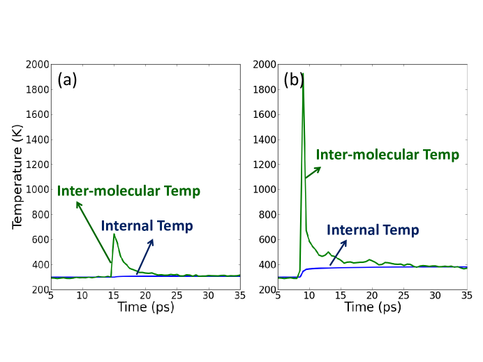
Figure 1: Time dependence of the local temperatures of a thin slab of HMX as a shock passes through with piston velocity u_p = (a) 0.4 km/s and (b) 1.0 km/s. We show inter-molecular and internal temperatures for mesodynamics simulation with coupling to internal modes.

III.3 Shock-induced temperature increase: quantum effects

Up to this point the thermal properties of the internal degrees of freedom have been treated classically. All-atom MD is always classical (in equilibrium, every DoF that appears squared in the Hamiltonian takes 1/2k_BT of energy) and, in order to compare with such results, we have used the classical harmonic approximation to obtain the specific heat for mesodynamics. However, classical statistical mechanics significantly overestimates the specific heat of molecular materials and we now use DID to assess the shock-induced heating when a correct quantum description is used.

Within the harmonic approximation, the internal modes of a molecule can be described by a set of N^int independent harmonic oscillators (normal modes) characterized by their frequency $\omega_{i}$; this is usually a good approximation for the internal degrees of freedom of a molecule in a wide temperature range and leads to analytical expressions for the specific heat both within classical and quantum mechanics. Classically, the internal energy of such harmonic system is given by: E${}^{int}_{CM}$=N^intk_BT and, as mentioned before, the specific heat is C${}^{int}_{CM}$=N^intk_B, where N^int is the number of normal modes. According to QM, the energy of a harmonic oscillator is given by: $e_{\omega_{i}}(n_{i})=\hbar\omega_{i}$ (1/2+n_i), where the quantun number n_i is an integer that gives the excitation of mode $i$, $\omega_{i}$ is its frequency and $\hbar$ is Planck’s constant. Using statistical mechanics we can calculate the average QM internal energy of a molecule at temperature T within the harmonic approximation:

$$E^{int}_{QM}(T) = \sum_{i=1}^{N^{int}}\frac{\sum_{n_{i}=0}^{\infty}e_{\omega_{i}}(n_{i})\exp[-e_{\omega_{i}}(n_{i})/kT]}{\sum_{n_{i}=0}^{\infty}\exp[-e_{\omega_{i}}(n_{i})/kT]}$$ (26)

$$= \sum_{i=1}^{N^{int}}\frac{1}{2}+\hbar\omega_{i}\frac{1}{\exp(\hbar\omega_{i}/kT)-1},$$

the specific heat is, thus:

$$C^{int}_{QM}(T)=k_{B}\sum_{i=1}^{N^{int}}\frac{\left(\hbar\omega_{i}/kT\right)^{2}\exp(\hbar\omega_{i}/kT)}{\left(1-\exp(\hbar\omega_{i}/kT)\right)^{2}}.$$ (27)

Since each mode can only take or give energy in a quantized manner (in lumps of $\hbar\omega_{i}$), high-frequency, high-energy modes are not excited at low temperatures and the specific heat is much smaller than the classical value. In Fig. 3 we show the temperature dependence of the specific heat of HMX calculated using Eq. 27 and normal mode frequencies obtained from the experimental data in Ref. brand02, .

Figure 2: Quantum and classical specific heats for HMX as a function of temperature.

While the thermal properties of all-atom MD simulations is always classical, our mesodynamic approach (Eqs. II.3 and II.3) enables the use of a quantum mechanically-derived, temperature dependent, specific heat to describe the thermal role of the internal DoFs. In Fig. 3 we show the time evolution of the internal temperature of a thin HMX slab as shockwaves with u_p=0.4 and 1.0 km/s pass through it using both classical (full lines) and quantum (dashed lines) specific heats. As expected, the smaller value of the quantum specific heat leads to higher shock temperatures and this effect is more marked for weaker shocks. For the shock with u_p = 1.0 km/s the temperature increase is underestimated by a factor of approximately two in a classical description (remember the mesodynamics with classical specific heat agrees well with all-atom MD). Interestingly, the quantum DID results are more accurate (within the limitations of the mesopotential and the input specific heat) than all-atom MD and classical mesodynamics.

The overestimation of the specific heat of materials below their Debye temperature by classical mechanics should be carefully acknowledged in the interpretation of MD simulations, especially of non-equilibrium processes like shock-induced chemical reactions strachan03 and thermal transport. donadio09 ; turney09

Figure 3: Time dependence of the internal temperatures of a thin HMX slab with classical and quantum specific heats and under shocks with u_p = 0.4, 1.0, and 2.0 km/s.

IV DID for electrons: thermal transport by electrons and phonons

Understanding nanoscale heat transport in metallic systems, where conduction electrons play a dominant role, is important for the applications in heat-assisted magnetic recording,Kryder08 microelectromechanical systems (MEMS),Bechtold05 ; Hyman99 ; Jensen05 high power laser,Huyeh08 ; Guo12 and thermoelectric devices.Harman02 ; Chen02 Challenges involved with direct experimental measurements at the nanoscale and the separation between the electronic and the phononic contributions make atomic simulations attractive. Standard all-atom MD simulations provide an explicit description of phonons but ignore the transport role of electrons and are, therefore, incapable of capturing thermal transport in metals.

To address this limitation the MD technique has been combined with the two-temperature model to simulate the thermal transport in metal and metal-semiconductor systems.Rutherford07 ; Duffy07 ; Phillips09 ; Wang12 ; Li09 In these simulations, electronic transport is described by solving the diffusion equation over a grid that overlaps with the atomic system. The two subsystems are coupled with local phonon temperature obtained from the atomic velocities.

In this Section, we apply DID to simulate the thermal transport in metals via the two-temperature model. Sub-section IV.2 shows verification tests of our implementation that also serve the purpose of exemplifying the use of the method. Sub-section IV.3 discusses thermal transport calculations in nanoscale Al focusing on the effects of specimen size and electron-phonon coupling rate.

IV.1 Simulation details

In this DID simulations particles represent Al atoms and their interaction is described by an embedded atom model potential Mishin02 . Conduction electrons are described as implicit DoFs. Since these electrons are not tied to the atoms, we include diffusive transport between them as described by Eq. IV.1. We repeat the equations here using elec to indicate electronic properties and atom for atomic ones :

$${\bf\dot{r}}_{i} = {\bf u}_{i}+\frac{\nu}{m_{i}\omega_{E}^{2}}\left(\frac{T^{atom}_{i}-T^{elec}_{i}}{T_{0}}\right){\bf F}_{i}\ ,$$

$${\bf\dot{u}}_{i} = \frac{{\bf F}_{i}}{m_{i}}\ ,$$

$$\dot{E}^{elec}_{i} = C^{elec}(T^{elec}_{i})\dot{T}^{elec}_{i}$$

$$= \frac{\nu}{m_{i}\omega_{E}^{2}}\left(\frac{T^{atom}_{i}-T^{elec}_{i}}{T_{0}}\right)|{\bf F}_{i}|^{2}+\kappa^{elec}\ \nabla^{2}T^{elec}_{i}\ .$$

In these equations, $\nu$ is the coupling rate between the electronic and atomic subsystems, and $\kappa^{elec}$ is the electronic thermal conductivity. Our DID approach to describe electronic thermal transport is similar to the MD two-temperature modelWang12 ; Duffy07 ; Rutherford07 except that the electronic temperatures are based on the atomic positions instead of the spatial grid and that the coupling is done via the position update equation. The benefit of using atomic positions as a grid for electron-phonon coupling is that the atomic structures at the interfaces and free surfaces can be captured accurately and in a straightforward manner.

We use coupling rates $\nu$ between 0.00017 ps^-1 and 0.017 ps^-1, corresponding to electron-phonon coupling constants of 0.01-1$\cdot 10^{17}$ $W/m^{3}K$. The electronic energy per atom, $E^{elec}$, is set to $7.975\cdot 10^{-5}\cdot{T^{2}}\cdot{k_{b}}$Dicke67 leading to a specific heat per atom $C^{elec}$ to be $1.595\cdot 10^{-4}\cdot k_{b}\cdot T$. The electronic thermal conductivity, $\kappa^{elec}$, is $27259.245\cdot k_{b}\cdot\AA^{2}/ps$, which is equivalent to 222 W/(mK)asm . $<\omega^{2}>$ is 39.783 ps^-2, which is obtained from the Debye temperature of Al.Bose09

IV.2 Verification tests

The DID equations of motion conserve total energy (the sum of the electronic and atomic subsystems) even when the energy is exchanged between the atoms and the electrons. To verify the energy conservation during the equilibration process between the atomic and electronic subsystems, an fcc Al system containing 4,000 atoms (5 x 5 x 40 unit cells) was used. For this system, the lattice constant is 0.408 nm, and the cell oriented along x = [100], y = [010], and z = [001]. Initial temperatures of 600K and 300K are assigned to the electronic and atomic subsystems and the equilibration process is followed via an isochoric-adiabatic (NVE) simulation for 20 ps. The atomic timestep is set to 0.1 fs and 40 electronic timesteps are performed per atomic timestep.

The equilibration between electronic and atomic temperatures with time for various coupling constants is shown in Figs. 4 (a-c) and the corresponding total and subsystem energies in Figs. 4 (d-f). Since the specific heat of atoms is much larger than that of electrons, the final equilibrium temperatures are close to, but slightly larger than, the initial atomic temperature. The role of coupling constant in equilibration time is clear from the figure. From Figs. 4 (d) and (e), the total energies of the systems are conserved during the equilibration process for systems with $\nu$ of 0.0017 ps^-1 and 0.00017 ps^-1. However, due to the very large energy exchange between electrons and atoms for the system with $\nu$ of 0.017 ps^-1, the total energy for this system drifts during the equilibration process, see Fig. 4 (f).

The time-evolution of electronic temperature is governed by the diffusion equation. To verify our implementation we set $\nu$ to 0.00 ps^-1 to decouple the atomic and electronic degrees of freedom and solve the time evolution of the electronic temperature given an initial Gaussian temperature profile. The initial electronic temperature is:

$$T_{i}^{elec}(t=0,z)=300+200\cdot exp\left(\frac{-(203.938-z)^{2}}{1600}\right)$$ (29)

With this initial condition we perform a DID simulation under isochoric-adiabatic (NVE) conditions using a temperature-independent electronic specific heat $C^{elec}=0.048711\cdot k_{b}$. The analytical solution of the time evolution of the temperature profile is:

$$T_{i}^{elec}(t,z)=300+\left(\frac{4000}{\sqrt{\alpha}}\right)exp\left(\frac{-(203.9-z)^{2}}{4\alpha}\right)$$ (30)

where $\alpha$ is equal to $\frac{\kappa^{elec}}{C^{elec}}(t+t_{0})$.

The DID temperature evolution is compared with the analytical solution in Fig. 5. The inset shows the width of the distribution, $\alpha$, as a function of time for both cases. In this simulation, the positions of moving atoms obtained from the equations of motion are used as a grid for the electronic temperatures, while the MD two-temperature model uses a fixed spatial grid to describe the electronic temperatures. The MD results agree with the analytical solutions for short simulation times when the periodic boundary conditions lead to negligible interactions between the temperature profiles in neighboring cells.

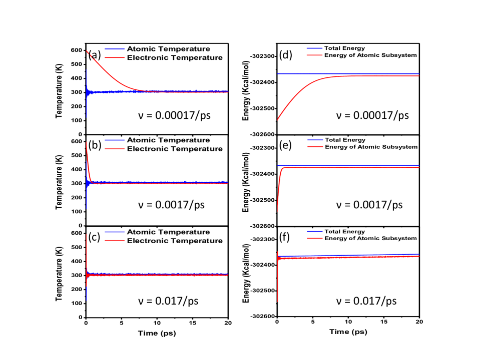
Figure 4: (a,b,c) Temperature equilibration between the electronic and atomic subsystems and (d,e,f) time evolution of the total and atomic energies for different electron-phonon coupling constants.

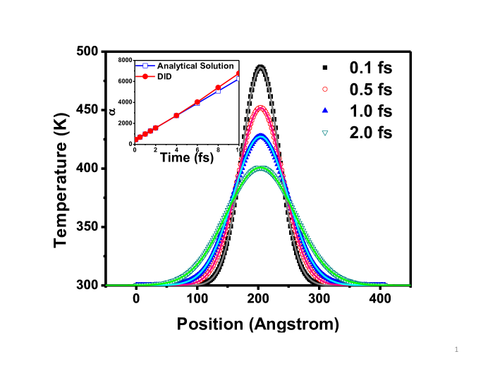
Figure 5: Electronic temperature profiles at different times without coupling to the atomic temperature. The points are the results from DID simulation and the solid lines are the results from analytical solution. Inset: broadening factor, $\alpha$ calculated from the analytical solution and from the electronic temperature evolution of DID simulation.

IV.3 Effect of size and electron-phonon coupling constant

We now use non-equilibrium DID simulations to study the role of specimen size and electron-phonon coupling constant, $\nu$, on the thermal conductivity of Al. We perform simulations on 3D periodic systems with size varying from 5 x 5 x 40 unit cells (4,000 atoms) to 5 x 5 x 400 unit cells (40,000 atoms) with coupling constants $\nu$ ranging from 0.00 ps^-1 to 0.017 ps^-1.

We compute thermal conductivity via non-equilibrium DID simulations with a method proposed by M$\ddot{u}$ller-Plathe method.MullerPlathe97 Heat fluxes in the range of $1-2\cdot 10^{11}W/m^{2}$ are introduced by periodically swapping the atomic velocities of the coldest atom in the hot bin (the first bin) and the hottest atom in the cold bin (the middle bin) every 10 fs (every 100 atomic timesteps). The total simulation time is 200 ps for systems with $\nu$ equal to 0.00 ps^-1 and the thermal conductivity is calculated from 100-200 ps. The total simulation time is 80 ps for systems with $\nu$ from 0.00017-0.017 ps^-1 and the thermal conductivity is calculated from 40-80 ps. In this method the thermal conductivity is computed using Fick’s law as the ratio between the temperature gradient and the heat flux. The temperature gradient is obtained from the linear fit to the effective temperature $T^{eff}$ of the whole material excluding the hot and cold bins. $T^{eff}$ is defined by both electronic and atomic subsystems via:

$$C^{total}(T^{eff})\cdot T^{eff}=C^{atom}\cdot T^{atom}+C^{elec}(T^{elec})\cdot T^{elec}$$ (31)

where $C^{atom}$ is the specific heat of atomic subsystem and is equal to $3\cdot k_{b}$ per atom, and $C^{total}$ is the total specific heat of the system. $T^{atom}$ and $T^{elec}$ are the temperatures of atomic and electronic subsystems, respectively.

The electronic and atomic temperature profiles of Al with $\nu$ from 0.00017-0.017 ps^-1 and specimen lengths from 16.32-163.20 nm are shown in Fig. 6. Due to the periodic kinetic energy exchange in the hot and cold bins, the temperatures of atoms and electrons remain out of equilibrium in these areas for all cases. For relatively long specimens and high coupling constants the atoms and electrons come to local equilibrium away from the energy-exchange zones, see Fig. 6. As will be shown below the thermal conductivity in such cases is approximately the phonon thermal conductivity (obtained as a function of size for the $\nu$=0.00 ps^-1 simulations) plus the electron one (208 W/(mK)). Interestingly, for smaller specimens or weaker electron-phonon coupling constants the electrons do not reach local thermal equilibrium with the atoms and do not fully participate in heat transport. Similar results have been shown by the theoretical calculations of two-temperature model with suitable boundary conditions. Ju06 ; Miranda11 From these theoretical studies,Ju06 ; Miranda11 the non-equilibrium behavior between electrons and atoms occurs at the metal-semiconductor interface, and as the thickness of metal layers increase, the electrons and atoms are in better equilibration inside the metal layers.

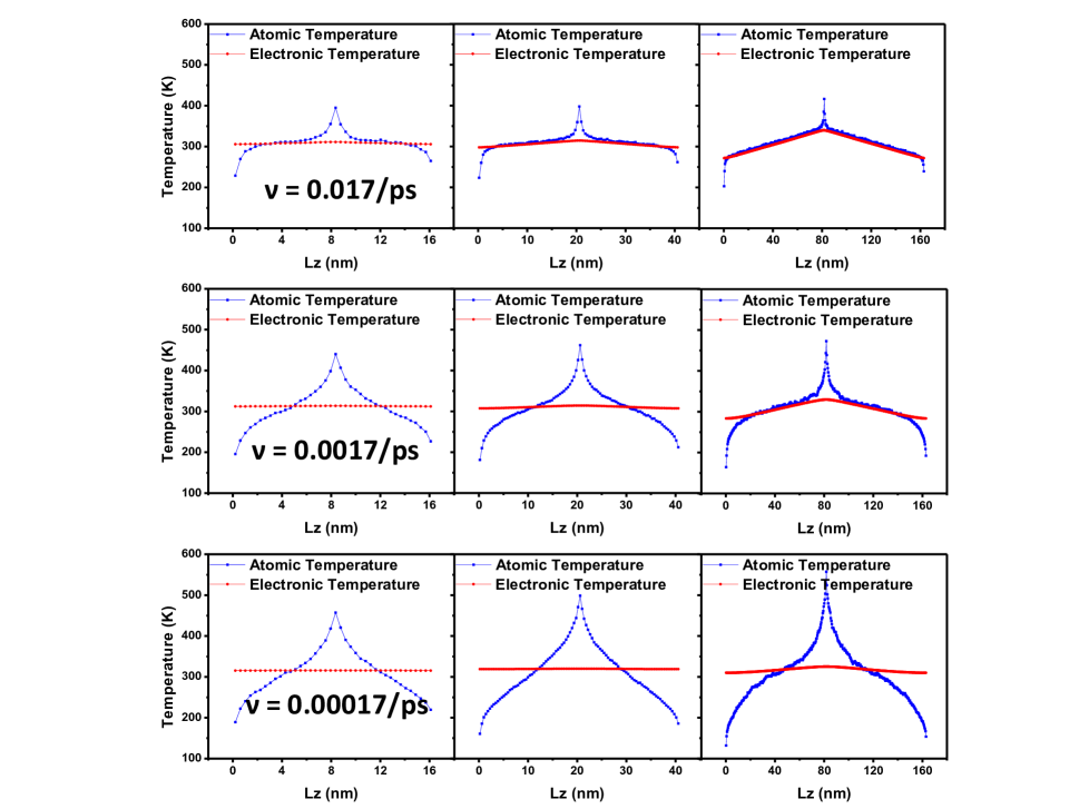
Figure 6: Steady-state electronic and atomic temperature profiles during non-equilibrium MD simulations for various electron-phonon coupling constants and specimen sizes.

Figure 7 shows the calculated thermal conductivity of the Al specimens as a function of their size for various coupling constants investigated. The ideal result of the atomic contribution (from the $\nu$=0.00 ps^-1 simulations) plus the input electronic thermal conductivity $\kappa^{elec}$ is shown as green open triangles. This value is only reached when electrons and atoms reach local equilibrium within the specimen. Even under steady state the heat exchange regions are driven away from equilibrium and local equilibrium within the sample is only achieved for relatively long specimens or large coupling constants. As the specimen size or the electron-phonon coupling rate is reduced the lack of local equilibration between the two subsystems leads to electrons contributing sub-optimally to thermal transport and a decrease in the effective thermal conductivity of the material. Similar effects have been observed in purely phononic transport in cases with different phonon groups remain away from local equilibrium Hu11 ; zhou13 .

This example shows the power of coupling a two-temperature description with MD simulations for ions can naturally capture non-diffusive effects and non-equilibrium processes.

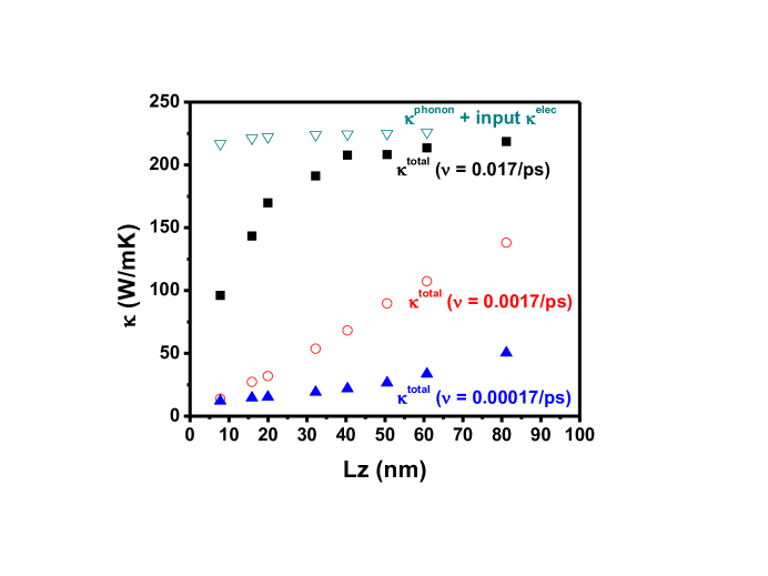
Figure 7: Thermal conductivity as a function of specimen length for various electron-phonon coupling constants. Green open triangles denote phonon thermal conductivity plus input electron value.

V Conclusions and Outlook

All particle-based simulations of materials describe explicitly only a limited set of degrees of freedom which are considered essential for the problem at hand; many other DoFs are treated in an approximate manner or their contributions disregarded altogether. This approximation puts severe constraints to the type of phenomena that can be described accurately by these methods.

In this paper we have presented the implementation of a thermodynamically accurate set of mesodynamics equations of motion that accurately describe the thermal and transport roles of the implicit DoFs. We applied this method to describe intra-molecular degrees of freedom in a mesoscale description of a polymer and to describe valence electrons in atomistic simulations of metallic systems. The mesodynamics enables for a quantum mechanical treatment of the thermal role of the implicit DoFs. This leads, in the case of molecular systems, to a mesoscopic description that is more accurate than the computationally more intensive all-atom MD (which is always classical).

The new thermo-mechanical formulation of mesodynamics presented in this paper is generally applicable, extending the spatial and temporal range of more expensive all-atom simulations to thermodynamically realistic mesoscopic simulations, with the possibility of solving a wide variety of problems in physics, chemistry, materials science, and biology.

Appendix A Thermostatted equations of motion

Under time-reversible integral feedback, thermo-mechanical mesodynamics can be formulated to give time averages that correspond to ensemble averages under isothermal, isochoric (NVT) conditions. Under the quasi-ergodic hypothesis, the long-time average of a quantity measured along a given many-body trajectory equals its average, at a given instant of time, over a multitude (ensemble) of such trajectories.

To obtain NVT equations of motion from Eqs. II.1, we first set the coupling between internal DoFs to zero, $\dot{\xi}_{i}=0$. Next, we take the range of the weighting function to be infinite ($w=1$), so that the external temperature of all mesoparticles is $T^{ext}_{i}=T$, and then set the number of internal DoFs to infinity, such that the internal (thermostat) temperature is fixed for all mesoparticles, $T^{int}_{i}=T_{0}$ (this represents the temperature of the heat bath). In that case, the heat-flow variable also takes on global character: $\zeta_{i}=\zeta$, and, instead of Eq.18, its equation of motion is derived from the requirement that the canonical ensemble distribution function be a stationary solution of the Liouville equation for the phase-space motion. We represent the $(2dN+1)$-dimensional phase space of coordinates and velocities by ${\bf x}=\{{\bf r},{\bf u};\zeta\}$; the equations of motion, $\dot{{\bf x}}({\bf x},t)=$

$${\bf\dot{r}}_{i} = {\bf u}_{i}+\frac{\nu\zeta}{m_{i}\omega_{E}^{2}}{\bf F}_{i}$$

$${\bf\dot{u}}_{i} = \frac{{\bf F}_{i}}{m_{i}}$$

$$\dot{\zeta} = ?$$ (32)

where the equation of motion for $\zeta$ is to be determined (see Ref. holian95, for a comparable treatment of Nosé-Hoover thermostatting).

The canonical distribution function (equilibrium) is

$$\rho_{0}=\frac{1}{Q_{0}}\ e^{-\beta E({\bf x})}\ ,$$ (33)

where $Q_{0}$ is the canonical partition function (normalization), $\beta=1/kT_{0}$, and the total system energy includes $\frac{1}{2}kT_{0}$ for the thermostat heat-flow variable $\zeta$, compared with $O(N)$ for the kinetic and potential contributions:

$$E({\bf x})=K(\{{\bf u}\})+\Phi(\{{\bf r}\})+\frac{d}{2}NkT_{0}\zeta^{2}\ .$$ (34)

The distribution function obeys the Liouville continuity equation in the (2d+1) dimensional phase space:

$$\frac{\partial\rho}{\partial{\bf t}}+\frac{\partial}{\partial{\bf x}}\cdot\left(\rho\dot{{\bf x}}\right)=0\ .$$ (35)

Since the equilibrium canonical distribution function does not explicitly depend on time (it is a stationary solution of the trajectories that make up the ensemble),

$$0 = \frac{\partial\rho_{0}}{\partial t}+\dot{{\bf x}}\cdot\frac{\partial\rho_{0}}{\partial{\bf x}}+\rho_{0}\frac{\partial}{\partial{\bf x}}\cdot\dot{{\bf x}}$$

$$= -\rho_{0}\beta\dot{E}+\rho_{0}\frac{\nu\zeta}{\omega_{E}^{2}}\sum_{i=1}^{N}\frac{1}{m_{i}}\frac{\partial}{\partial{\bf r}_{i}}\cdot{\bf F}_{i}$$

$$\Rightarrow\dot{E} = -dNkT_{0}\nu\zeta\ \frac{\omega^{2}}{\omega_{E}^{2}}\ ,$$ (36)

where we imposed the condition that $\dot{\zeta}$ does not depend on $\zeta$ itself.

Substituting the equations of motion (Eqs. A) into Eq.A, we find that

$$\dot{E} = \sum_{i}m_{i}\dot{{\bf u}}_{i}\cdot{\bf u}_{i}+\sum_{i}\frac{\partial\Phi}{\partial{\bf r}_{i}}\cdot\dot{{\bf r}}_{i}+dNkT_{0}\ \zeta\dot{\zeta}$$

$$= \sum_{i}{\bf F}_{i}\cdot{\bf u}_{i}-\sum_{i}{\bf F}_{i}\cdot\left({\bf u}_{i}+\frac{\nu\zeta}{m_{i}\omega_{E}^{2}}{\bf F}_{i}\right)+dNkT_{0}\ \zeta\dot{\zeta}$$

$$= -\frac{\nu\zeta}{\omega_{E}^{2}}\ \sum_{i}\frac{|{\bf F}_{i}|^{2}}{m_{i}}+dNkT_{0}\ \zeta\dot{\zeta}$$

$$\Rightarrow\dot{\zeta} = \nu\left(\frac{1}{dNkT_{0}\omega_{E}^{2}}\ \sum_{i}\frac{|{\bf F}_{i}|^{2}}{m_{i}}-\frac{\omega^{2}}{\omega_{E}^{2}}\right)\ .\$$ (37)

At long times, the equation of motion for the heat-flow variable $\zeta$ gives a time average equal to zero:

$$\overline{\dot{\zeta}} = \lim_{t\rightarrow\infty}\ \frac{1}{t}\int_{0}^{t}\ ds\ \frac{d\zeta}{ds}=\lim_{t\rightarrow\infty}\ \frac{\zeta(t)-\zeta(0)}{t}=0$$ (38)

$$\Rightarrow \overline{\omega^{2}}=\frac{1}{dNkT_{0}}\ \sum_{i}\frac{\overline{|{\bf F}_{i}|^{2}}}{m_{i}}\ .$$

We can evaluate the canonical ensemble average of the mean-square frequency as follows:

$$\langle\omega^{2}\rangle = \frac{1}{Q_{0}}\prod_{j}\int_{V}d{\bf r}_{j}e^{-\beta\Phi}\ \frac{1}{dN}\ \sum_{i}\frac{1}{m_{i}}\frac{\partial}{\partial{\bf r}_{i}}\cdot\frac{\partial\Phi}{\partial{\bf r}_{i}}$$ (39)

$$= \frac{1}{d}\int_{V}d{\bf r}e^{-\beta\Phi}\frac{1}{m}\frac{\partial}{\partial{\bf r}}\cdot\frac{\partial\Phi}{\partial{\bf r}}\ {\Big{/}}\int_{V}d{\bf r}e^{-\beta\Phi}\ ,$$

where integration by parts (with the surface term equal to zero under periodic boundary conditions) yields

$$\int_{V}d{\bf r}e^{-\beta\Phi}\frac{1}{m}\frac{\partial}{\partial{\bf r}}\cdot\frac{\partial\Phi}{\partial{\bf r}} = \frac{1}{m}\frac{\partial\Phi}{\partial{\bf r}}\cdot\hat{{\bf n}}_{S}e^{-\beta\Phi}{\Big{|}}_{-S}^{+S}$$ (40)

$$-\ \int_{V}d{\bf r}\frac{1}{m}\frac{\partial\Phi}{\partial{\bf r}}\cdot\frac{\partial}{\partial{\bf r}}e^{-\beta\Phi}$$

$$= \beta\int_{V}d{\bf r}\frac{1}{m}\frac{\partial\Phi}{\partial{\bf r}}\cdot\frac{\partial\Phi}{\partial{\bf r}}e^{-\beta\Phi}$$

$$= \beta\int_{V}d{\bf r}e^{-\beta\Phi}\frac{|{\bf F}|^{2}}{m}\ ,$$

so that

$$\langle\omega^{2}\rangle=\frac{1}{dNkT_{0}}\sum_{i}\frac{\langle|{\bf F}_{i}|^{2}\rangle}{m_{i}}\ ,$$ (41)

this relation between $\langle\omega^{2}\rangle$, the temperature and force squared can also be obtained from the velocity power spectrum.

We see, therefore, that mesodynamics thermalization can be specialized to global canonical thermostatting, where the equations of motion satisfy the quasiergodic hypothesis: $\omega_{E}^{2}=\overline{\omega^{2}}=\langle\omega^{2}\rangle$.

From these results, it is tempting to postulate a new definition of instantaneous temperature $\tilde{T}$, written in such a way as to easily identify mass times velocity-squared (see the definition of the dissipative terminal velocity in Eq.II),

$$dk\tilde{T}=\frac{1}{N}\sum_{i}m_{i}{\Big{|}}\frac{{\bf F}_{i}}{m_{i}\omega_{E}}{\Big{|}}^{2}\ ,$$ (42)

by analogy with the usual kinetic definition $T$ (see, e.g., Eq.2, with the weighting function set to $w\equiv 1$),

$$dkT=\frac{1}{N}\sum_{i}m_{i}|{\bf u}_{i}-\langle{\bf u}\rangle|^{2}\ .$$ (43)

$\langle{\bf u}\rangle$ is the c.m. velocity of the system (see e.g., Eq.1). However, defining the temperature in terms of forces differs instantaneously from that defined by velocities, as can be exemplified most clearly by hard spheres: most of the time, the forces are zero as particles move in straight-line, constant-velocity trajectories between collisions; at the moment of collisions, forces are formally infinite and velocities are zero; therefore, the two definitions of “instantaneous” temperature are starkly different, though their running time-averages do approach each other, as can be seen from Eq.A, into which we substitute the new temperature definition of Eq.42:

$$\dot{\zeta}=\nu\left(\frac{\tilde{T}}{T_{0}}-\frac{\omega^{2}}{\omega_{E}^{2}}\right)\ ,$$ (44)

and where the long-time average gives $\overline{\tilde{T}}=T_{0}$.

Notice that this mesodynamics approach to the canonical ensemble does not at all replace the Nosé-Hoover (NH) approach to bulk thermostatting NH , though Eq.44 bears a strong resemblance to the latter’s equation of motion for the heat-flow variable. For one thing, the mesodynamics version requires an expensive evaluation of the Hessian (curvature) of the potential energy; moreover, two force evaluations per central-difference time-step are required: one for the coordinate update, and one for the velocity update. Thus, the traditional NH thermostat is at least twice as computationally efficient as the one derived from mesodynamics.

While the derivation of the canonical thermostat from mesodynamics that we have presented here is only of academic interest, it shows nevertheless, that the thermo-mechanical foundations of mesodynamics are deep. On the other hand, the need for twice the number of force evaluations is simply the price that has to be paid for Galilean invariance of the equations of motion.

Appendix B Finite central-difference approximation to the mesodynamics equations of motion

In this Appendix, we display the finite central-difference equations (originally the Størmer method, which was “rediscovered” by Vineyard vineyard —but also known commonly in the modern literature as the “Verlet” method); the computational time-step is $\delta$. In general, coordinates are computed at integer time-steps, while velocities are computed at half-integer values. In common parlance, this is called the “leap-frog” method, since, in the update of either coordinate or velocity, the time derivative is evaluated halfway in between the new and old time-steps. The time derivatives are always computed at least to $O(\delta^{2})$, which when multiplied by $\delta$ give errors in the Taylor series that are formally of $O(\delta^{3})$. When the updates of velocities and coordinates, via the first-order ordinary differential equations (o.d.e.’s), are combined into second-order o.d.e.’s for coordinates alone, the local error in the finite central-difference equations are $O(\delta^{4}$); central differences are referred to as a second-order integration method.

In this paper, the mesodynamics equations of motion are presented in two flavors: (1) integral feedback in Eqs.II.3 and (2) direct feedback in Eqs.B. (For simplicity in the following development, we drop the vector notation for coordinates, velocities, and forces, as well as the mesoparticle index $i$.) The equation of motion for the energy of the internal degrees of freedom can be easily generalized for a heat capacity that depends on internal temperature as a power law, namely, $C_{V}=CT^{n}$ (the most interesting cases are $n=0$, where $C_{V}$ is independent of $T$, and $n=1$, which is appropriate for low-temperature metals); hence, $\dot{E}^{int}=(n+1)C_{V}\dot{T}^{int}$. Therefore, we set $C_{V}^{\prime}=(n+1)C_{V}$ and $\lambda^{\prime}=\lambda/(n+1)$, where $\lambda=\kappa/C_{V}$ is the thermal diffusivity.

In the integral feedback version, the mesodynamics difference equations [formally to $O(\delta^{3})$] are given by:

$$r(t) = r(t-\delta)+\chi(t-\frac{\delta}{2})F(t-\frac{\delta}{2})\delta$$

$$u(t+\frac{\delta}{2}) = u(t-\frac{\delta}{2})+\frac{F(t)}{m}\delta$$

$$T^{int}(t+\frac{\delta}{2}) = T^{int}(t-\frac{\delta}{2})+\frac{\chi(t)|F(t)|^{2}}{C_{V}^{\prime}}\delta$$

$$+\ \frac{\nu_{0}\xi(t)}{C_{V}^{\prime}}\delta$$

$$\zeta(t+\delta) = \zeta(t)+\nu\frac{T^{ext}(t+\frac{\delta}{2})-T^{int}(t+\frac{\delta}{2})}{T_{0}}\delta$$

$$\xi(t+\delta) = \xi(t)+\kappa\nabla^{2}T^{int}(t+\frac{\delta}{2})\delta\ ,$$ (45)

where $\chi=\nu\zeta/m\omega_{E}^{2}$ and $T_{0}$ is an arbitrary temperature (the initial value of $T^{int}$, for example). The auxiliary flow variables $\zeta$ and $\xi$ are most naturally evaluated at integer time-steps; whenever they appear with half-integer values of time in the above equations, they are being used in mid-point time derivatives, so that they can be evaluated as averages over the neighboring integer time-steps: for example,

$$\zeta(t+\frac{\delta}{2})=\frac{1}{2}\left[\zeta(t)+\zeta(t+\delta)\right]+O(\delta^{2})\ .$$ (46)

In the coordinate update (the first line of Eq.B), the force that appears must be evaluated at the end of the previous time-integration cycle—the temporary coordinates used to compute the forces are evaluated to $O(\delta^{2})$ and stored as temporary values—thereupon, the force is evaluated and stored for the next time-step. Thus, the force needs to be evaluated twice in each time-step cycle, rather than just once, as is usual in standard molecular-dynamics simulations.

The direct feedback version of the central-difference equations is given by

$$r(t) = r(t-\delta)+\chi(t-\frac{\delta}{2})F(t-\frac{\delta}{2})\delta$$

$$u(t+\frac{\delta}{2}) = u(t-\frac{\delta}{2}))+\frac{F(t)}{m}\delta$$

$$T^{int}(t+\frac{\delta}{2}) = T^{int}(t-\frac{\delta}{2})+\frac{\chi(t)|F(t)|^{2}}{C_{V}^{\prime}}\delta$$ (47)

$$+\ \lambda^{\prime}\nabla^{2}T^{int}(t)\delta\ ,$$

where $\chi=\nu(T^{ext}-T^{int})/T_{0}$. Note that the heat conduction term (Fourier’s Law) needs an estimate (a temporary variable) for $T^{int}(t)$ that is accurate to $O(\delta^{2})$:

$$T^{int}(t) = T^{int}(t-\frac{\delta}{2})+\frac{\chi(t)|F(t)|^{2}}{C^{\prime}}\frac{\delta}{2}$$ (48)

$$+\ \lambda^{\prime}\nabla^{2}T^{int}(t-\frac{\delta}{2})\frac{\delta}{2}\ ,$$

from which $\nabla^{2}T^{int}(t)$ is then computed for use in Eq.II.3.

References

- (1) B.J. Alder and T.E. Wainwright, J. Chem. Phys. 31, 459 (1959).
- (2) J.B. Gibson, A.N. Goland, M. Milgram, and G.H. Vineyard, Phys. Rev. 120, 1229 (1960).
- (3) G.A. Bird, Molecular Gas Dynamics and the Direct Simulation of Gas Flows (Clarendon, Oxford, 1994).
- (4) T.C. Germann and K. Kadau, Int. J. Modern Phys. C 19, 1315 (2008).
- (5) B.L. Holian, Europhys. Lett. 64, 330 (2003).
- (6) H. Häkkinen and U. Landman, Phys. Rev. Lett. 71, 1023 (1993).
- (7) F. Müller-Plathe, J. of Chem. Phys. Chem. 3, 754 (2002); K. Fremer, Macromol. Chem. Phys. 204, 257 (2003).
- (8) G. Stoltz, Europhys. Lett. 76, 849 (2006).
- (9) J.B. Maillet, L. Soulard, and G. Stoltz, EPL 78, 68001 (2007).
- (10) L. Lucy, Astron. J. 82, 1013 (1977); J.J. Monaghan, Ann. Rev. Astron. Astrophys. 30, 543 (1992).
- (11) O. Kum, W.G. Hoover, H.A. Posch, Phys. Rev. E 52, 4899 (1995).
- (12) J.J. Monaghan, J. Comp. Phys. 82, 1 (1989); J.P. Gray, J.J. Monaghan, and R.P. Swift, Comp. Meth. Appl. Mech. Eng. 190, 6641 (2001).
- (13) M.S. Daw and M.I. Baskes, Phys. Rev. Lett. 50, 1285 (1983).
- (14) O.B. Firsov, Sov. Phys.-JETP 36, 1076 (1959); M. Moseler, J. Nordieck, and H. Haberland, Phys. Rev. B 23, 15439 (1997).
- (15) A. Strachan and B.L. Holian, Phys. Rev. Lett. 94, 014301 (2005).
- (16) H. Berendsen, J. Postma, W. van Gunsteren, A. Dinola, J. Haak, J. Chem. Phys. 81, 3684 (1984).
- (17) S. Nosé, J. Chem. Phys. 81, 511 (1984); W.G. Hoover, Phys. Rev. A 31, 1695 (1985).
- (18) B.L. Holian, A.F. Voter, and R. Ravelo, Phys. Rev. E 52, 2338 (1995).
- (19) T. Furukawa, Phase Transitions 18, 143 (1989).
- (20) N. Karasawa, and W. A. Goddard III, Macromolecules 25, 7168 (1992).
- (21) A. Majumdar and P. Reddy, Appl. Phy. Lett. 84, 4768 (2004).
- (22) Y. Ju, M.-T. Hung and T. Usui, J. Heat Trans. 128, 919 (2006).
- (23) J. Ordonez-Miranda, J.J. Alvarado-Gil and R. Yang, J. Appl. Phys. 109, 094310 (2011).
- (24) A.M. Rutherford and D.M. Duffy, J. Phys.: Condens. Matter 19, 496201 (2007).
- (25) D.M. Duffy and A.M. Rutherford, J. Phys.: Condens. Matter 19, 016207 (2007).
- (26) C.L. Phillips and P.S. Crozier, J. Chem. Phys. 131, 074701 (2009).
- (27) Y. Wang, X. Ruan and A.K. Roy, Phys. Rev. B 85, 205311 (2012).
- (28) X. Li, L. Jiang and H.-L. Tsai, J. Appl. Phys. 106, 064906 (2009).
- (29) Y. Mishin, M.J. Mehl, and D.A. Papaconstantopoulos, Phys. Rev. B 65, 224114 (2002).
- (30) D.A. Dicke and B. A. Green, Jr., Phys. Rev. 153, 800 (1967).
- (31) Alloy Digest, ASM International (2002).
- (32) S.K. Bose, J. Phys.: Condens. Matter 21, 025602 (2009).
- (33) F. Müller-Plathe, J. Chem. Phys. 106, 6082 (1997).
- (34) K. Lynch, A. Thompson, and A. Strachan, Modelling Simul. Mater. Sci. Eng. 17, 015007 (2009).
- (35) E. Jaramillo, T. D. Sewell, and A. Strachan, Phys. Rev. B 76, 064112 (2007).
- (36) H. V. Brand, R. L. Rabie, D. J. Funk, I. Diaz-Acosta, P. Pulay and T. K. Lippert, J. Phys. Chem. B 106, 10594 (2002).
- (37) A. Strachan, A. van Duin, D. Chakraborty, S. Dasgupta, and W. A. Goddard, Phys. Rev. Lett. 91, 098301 (2003)
- (38) D. Donadio and G. Galli, Phys. Rev. Lett. 102, 195901 (2009)
- (39) J. E. Turney, A. J. H. McGaughey and C. H. Amon, Phys. Rev. B 79, 224305 (2009)
- (40) Y. Zhou and A. Strachan, J. Chem. Phys. 138, 124704 (2013)
- (41) L. Hu, T. Desai, and P. Keblinski, Phys. Rev. B 83, 195423 (2011)
- (42) M. H. Kryder, E. C. Gage, T. W. McDaniel, W. A. Challener, R. E. Rottmayer, G. Ju, Y.-T. Hsia, and M. F. Erden, Proceedings of the IEEE 96, 1810 (2008)
- (43) T. Bechtold, E. B. Rudnyi, and J. G. Korvink, J. Micromech. Microeng. 15, R17 (2005)
- (44) D. Hyman and M. Mehregany, IEEE Transactions on Components and Packaging Technology 22, 357 (1999)
- (45) B. D. Jensen, L. L.-W. Chow, K. Huang, K. Saitou, J. L. Volakis, and K. Kurabayashi, Journal of Microelectromechanical Systems 14, 935 (2005)
- (46) M. Rashidi-Huyeh, S. Volz, and B. Palpant, Physical Review B 78, 125408 (2008)
- (47) L. Guo, S. L. Hodson, T. S. Fisher and X. Xu, Journal of Heat Transfer 134, 042402 (2012)
- (48) T. C. Harman, P. J. Taylor, M. P. Walsh and B. E. LaForge, Science 297, 2229 (2002)
- (49) G. Chen and A. Shakouri, Transactions of the ASME 124, 242 (2002)
- (50) Y. Zhou and A. Strachan, J. Chem. Phys. 131, 234113 (2009)
- (51) E. Antillon, K. Banlusan and A. Strachan, Modelling Simul. Mater. Sci. Eng. 22, 025027 (2014)