Finite temperature spin dynamics in a perturbed quantum critical Ising chain with an $E_{8}$ symmetry

Abstract

A spectrum exhibiting $E_{8}$ symmetry is expected to arise when a small longitudinal field is introduced in the transverse-field Ising chain at its quantum critical point. Evidence for this spectrum has recently come from neutron scattering measurements in cobalt niobate, a quasi-one-dimensional Ising ferromagnet. Unlike its zero-temperature counterpart, the finite-temperature dynamics of the model has not yet been determined. We study the dynamical spin structure factor of the model at low frequencies and nonzero temperatures, using the form factor method. Its frequency dependence is singular, but differs from the diffusion form. The temperature dependence of the nuclear magnetic resonance (NMR) relaxation rate has an activated form, whose prefactor we also determine. We propose NMR experiments as a means to further test the applicability of the $E_{8}$ description for CoNb₂O₆.

Introduction.—

Quantum criticality is a subject of extensive interest in various contexts JLTP-issue10 ; sachdev . These range from correlated-electron bulk materials, which can be tuned to the border of magnetism, to systems in low dimensions, where quantum fluctuations are enhanced. The collective fluctuations of a quantum critical point (QCP) often lead to unusual properties. Even in equilibrium, the statics and dynamics are mixed at a QCP. This gives rise to dynamical scaling, while also making it difficult to calculate the fluctuation spectrum. The latter is especially so for the dynamics at nonzero temperatures ($T>0$) in the “quantum relaxational” regime, which corresponds to small frequencies ($\omega\ll k_{B}T/\hbar$) or long times. Indeed, even for the canonical QCP of a transverse-field Ising model in one dimension, it has been challenging to calculate such real-frequency dynamics deift ; sachdev2 .

We are interested here in the one dimensional transverse field Ising model in the presence of a small longitudinal field. The transverse-field-induced QCP in the absence of a longitudinal field pfeuty has an emergent conformal invariance in the scaling limit belavin . When a small longitudinal field is turned on at the QCP, the excitation spectrum becomes discrete at low energies. The perturbed conformal field theory zamolodchikov provided evidence that certain properties of the spectrum of the resulting relativistic field theory and the scattering matrix can be organized in terms of $E_{8}$, an exceptional simple Lie group of rank $8$. The discrete spectrum corresponds to eight particles, whose masses form ratios which are related to the roots of the $E_{8}$ algebra. (For introductory discussions, see Refs. dorey ; borthwick .) The first two particles describe bound states that are well below the continuum part of the spectrum. Recently neutron scattering measurements have been carried out in a ferromagnetic cobalt niobate CoNb₂O₆, whose Co²⁺ are coupled in a quasi-1D way; the experiment identified two excitations whose energy ratios are close to the predicted value, the golden ratio coldea .

In this letter, we study the low-frequency dynamical spin structure factor at finite temperatures using the form factor method mussardo . From a theoretical perspective, our calculation provides an illustrative setting to determine the dynamics in the quantum-relaxational regime. For the $E_{8}$ model, the dynamics at finite temperatures have not been systematically studied. From the perspective of the material CoNb₂O₆, our study determines the temperature dependence of the NMR relaxation rate. We note that our results bear some similarities with those for another model, the O(3) non-linear sigma model SagiAffleck ; Konik03 , although our study here benefits from the exactly regularized form factor series pozsgay ; szecsenyi . We also note that a numerical analysis of a generalized transverse-field Ising chain suggests that the E₈ description survives suitable generalizations of the interactions beyond the nearest-neighbor ferromagnetic coupling kjall .

The Model.—

Consider the Hamiltonian

$$H_{Z}=-J\left({\sum\limits_{i}{\sigma_{i}^{z}\sigma_{i+1}^{z}}+g\sum\limits_{i}{\sigma_{i}^{x}}+h_{z}\sum\limits_{i}{\sigma_{i}^{z}}}\right),$$ (1)

where $\sigma_{i}^{x}$ and $\sigma_{i}^{z}$ are the Pauli matrices associated with the spin components $S^{\mu}=\sigma^{\mu}/2,({\mu=x,y,z})$, and $i$ marks a site position, in addition $g$ and $h_{z}$ are the physical transverse and longitudinal fields, respectively, in unit of the nearest-neighbor ferromagnetic exchange coupling $J$ between the longitudinal ($z$) components of the spins. In the absence of the longitudinal field ($h_{z}=0$) the system undergoes a quantum phase transition when the transverse field is tuned across its critical value $g=g_{c}=1$ pfeuty . As is well known, the QCP is described by a $1+1$-dimensional conformal field theory (CFT) with a central charge $1/2$ belavin . More surprising is what happens when a small longitudinal field $h_{z}$ is introduced at the QCP $g=g_{c}$. The action in the continuum limit is given by:

$$\mathcal{A}_{E8}=\mathcal{A}_{c=1/2}+h\int dxd\tau\sigma(\tau,x).$$ (2)

This is an integrable field theory, and is referred to as the $E_{8}$ model because of the aforementioned connection between its properties and the $E_{8}$ group zamolodchikov ; mussardo . In the above equation, $\tau$ is the imaginary time, $\mathcal{A}_{c=1/2}$ stands for the action of the two dimensional CFT with central charge $1/2$, and $\sigma(x)$ is a primary field with scaling dimension $1/8$. In addition, $h=cJh_{z}/a$, where $a$ is the lattice constant and $c\approx 0.783$ converts between the $\sigma$ field of the continuum theory and its lattice counterpart $\sigma^{z}$ delfino1 . This describes a scattering theory of eight massive particles, which we will denote by $a,b,c,d,e,f,g,h$ from the lightest to the heaviest. The mass of the lightest particle, $\Delta_{a}$, scales with the longitudinal field as $\Delta_{a}\approx 4.405\left|h\right|^{8/15}$ mass . The mass of the second lightest particle $\Delta_{b}$ is $\Delta_{a}$ multiplied by the golden ratio $(\sqrt{5}+1)/2$. These two particles are clearly separated from the two-particle continuum, which appears at energies above $2\Delta_{a}$.

Local dynamics and NMR relaxation rate.—

We focus on the local dynamical structure factor (DSF) of the $E_{8}$ model in the low frequency and low temperature limit: $\omega\ll\Delta_{a}$ and $T\ll\Delta_{a}$ (hereafter we set $\hbar=1$ and $k_{B}=1$).

A useful means to probe the local DSF is via NMR. The NMR relaxation rate is given by moriya

$$\frac{1}{{T_{1}^{\alpha}}}=\frac{1}{{2N}}A^{2}\sum_{\beta}{}^{{}^{\prime}}S_{\beta\beta}(\omega_{0}).$$ (3)

Here, $\alpha$ and $\beta$ label the principal axes, and the primed summation is over the principal axes perpendicular to the field orientation $\alpha$; $T_{1}^{\alpha}$ is the spin-lattice relaxation time, $N$ is the number of ions per unit cell, and $\omega_{0}$ is the nuclear resonance frequency. In addition, $A$ describes the hyperfine coupling between the spins of a nucleus and the electrons; while this coupling depends on the wavevector ${\bf q}$, the dependence is generically smooth and we will take it as a constant. We will consider the static field of the NMR setup to be the transverse field, $\alpha=x$. Correspondingly, the local DSF of interest to NMR is given by $S_{zz}(\omega_{0})+S_{yy}(\omega_{0}).$ As shown in the supplementary materials supplement , for the model we consider,

$$S_{yy}(\omega)=\omega^{2}S_{zz}(\omega)/(4J^{2}).$$ (4)

Thus, in the low-frequency regime of interest here, $S_{yy}(\omega)$ is negligible compared with $S_{zz}(\omega)$. In the following, we will therefore only consider $S_{zz}$.

We now turn to the calculation of $S_{zz}(\omega)$ through a systematic form factor expansion. Because the excitation spectrum has a gap, we expect that the leading contributions in the low temperature and low frequency limit come from those associated with the few particle states of the light particles. Indeed, we show below that the dominant contribution comes from the two 1-particle states of the lightest particle, which we calculate analytically. The conclusion is confirmed by a numerical calculation for contributions that extend to higher orders.

The form factor series.—

Integrable field theory techniques made possible the analytic calculation of matrix elements of local observables in the asymptotic scattering state basis, called form factors. The asymptotic states are eigenstates of the energy and momentum operators. It is convenient to use the standard reparameterization in relativistic theories of a particle’s energy and momentum through the rapidity of the particle. In terms of the rapidities $\{\theta_{i}\}$ of the particles, the energy and momentum eigenvalues of the eigenstate $\left|{\theta_{1}^{\alpha_{1}},\cdots,\theta_{n}^{\alpha_{n}}}\right\rangle$ (with $\{\alpha_{1},\cdots,\alpha_{n}\}$ marking different types of particles) are

$$E_{n} =\sum_{i=1}^{n}\Delta_{\alpha_{i}}\cosh(\theta_{i}),$$ (5)

$$P_{n} =\sum_{i=1}^{n}\Delta_{\alpha_{i}}\sinh(\theta_{i}).$$ (6)

We denote by $F_{n}^{\sigma}(\theta_{1}^{\alpha_{1}},\cdots,\theta_{n}^{\alpha_{n}})$ the form factors of the primary field $\sigma(t,x)$ in the $E_{8}$ model (c.f. Eq. (2)) between the vacuum and an $n$-particle asymptotic state,

$$F_{n}^{\sigma}(\theta_{1}^{\alpha_{1}},\cdots,\theta_{n}^{\alpha_{n}})=\left\langle 0\right|\sigma(0,0)\left|{\theta_{1}^{\alpha_{1}},\cdots,\theta_{n}^{\alpha_{n}}}\right\rangle.$$ (7)

The few-particle form factors are explicitly known delfino1 ; delfino2 ; delfino3 and have been used to calculate the static spin-spin correlations of the $E_{8}$ model in the ground state delfino1 ; delfino2 . Here we study the finite-temperature dynamics by a low-temperature expansion series for integrable field theory essler ; pozsgay , using a finite-volume regularization pozsgay .

The finite temperature two-point correlation function is given by

$$C(t,x)=\mathrm{Tr}\left[\frac{e^{-H/T}}{\mathcal{Z}}\mathcal{O}(t,x)\mathcal{O}^{\dagger}(0,0)\right],$$ (8)

where $\mathcal{Z}=\mathrm{Tr}\,e^{-H/T}$ is the partition function, and we are interested in the local observable operator $\mathcal{O}(t,x)=\sigma(t,x)$ . The corresponding DSF is

$$S(\omega,q)=\int_{-\infty}^{\infty}{dx\int_{-\infty}^{\infty}{dt\;C(t,x)e^{i\omega t-iqx}}},$$ (9)

We insert the complete set of asymptotic states between the operators, yielding a double sum, $C(t,x)=\mathcal{Z}^{-1}\sum_{r,s}C_{r,s}(t,x)$, where

$$C_{r,s}(t,x)=\sum\limits_{\left\{{\alpha_{j}}\right\},\left\{{\alpha^{\prime}_{k}}\right\}}{\int{\frac{{d\theta_{1}\cdots d\theta_{r}}}{{(2\pi)^{r}r!}}\int{\frac{{d\theta^{\prime}_{1}\cdots d\theta^{\prime}_{s}}}{{(2\pi)^{s}s!}}}}}e^{-\beta E_{r}}\\ e^{-it(E_{s}-E_{r})}e^{-i(P_{r}-P_{s})x}\left|{\left\langle{\theta_{1}^{\alpha_{1}}\cdots\theta_{r}^{\alpha_{r}}}\right|\mathcal{O}\left|{\theta^{\prime}{{}_{1}^{\alpha^{\prime}_{1}}}\cdots\theta^{\prime}{{}_{s}^{\alpha^{\prime}_{s}}}}\right\rangle}\right|^{2}.$$ (10)

We use the same set of states to write the partition function as $\mathcal{Z}=\sum_{n=0}^{\infty}\mathcal{Z}_{n}$ where

$$\mathcal{Z}_{n}=\sum_{\{\alpha_{j}\}}\int\frac{d\theta_{1}\cdots d\theta_{n}}{(2\pi)^{n}n!}e^{-\beta E_{n}}\left\langle\theta_{1}^{\alpha_{1}}\cdots\theta_{n}^{\alpha_{n}}\right|\theta_{1}^{\alpha_{1}}\cdots\theta_{n}^{\alpha_{n}}\rangle.$$ (11)

In infinite volume all the $\mathcal{Z}_{n}$’s contain singularities associated with the scalar product of two momentum eigenstates with identical rapidities. Similarly, for the observables we are calculating, $C_{r,s}$ also diverge due to the kinematical poles of the form factors whenever two rapidities in the two sets coincide, $\theta_{i}=\theta^{\prime}_{j}$ essler . However, the double sums can be re-organized such that the aforementioned singularities cancel each other pozsgay ,

$$C(t,x)=\sum_{r,s=0}^{\infty}D_{r,s}(t,x)\,,$$ (12)

where

$$D_{0,s} =C_{0,s}\,,$$ (13)

$$D_{1,s} =C_{1,s}-\mathcal{Z}_{1}C_{0,s-1}\,,$$ (14)

$$D_{2,s} =C_{2,s}-\mathcal{Z}_{1}C_{1,s-1}+(\mathcal{Z}_{1}^{2}-\mathcal{Z}_{2})C_{0,s-2},$$ (15)

…etc. (16)

The natural small parameter in the series (12) is $e^{-\Delta_{a}/T}$. At low frequencies, the energy conserving Dirac-deltas in the Fourier transform Eq. (9) force the two states appearing in the form factors to have nearly equal energy, $E_{r}=\omega+E_{s}$. The magnitude of the Boltzmann factor is then set by the sum of the masses in the “heavier” state, i.e.,

$$D_{r,s}\sim\exp\left\{{-\frac{1}{T}\max\left[{\sum\limits_{i=1}^{r}{\Delta_{i}},\sum\limits_{i=1}^{s}{\Delta_{i}}}\right]}\right\}.$$ (17)

Thus, in the regime of interest ($T/\Delta_{a}\ll 1$ and $\omega/\Delta_{a}\ll 1$), the expansion series in Eq. (12) is a good perturbation series. In this regime, we can safely truncate the series beyond the terms up to the order of $e^{-2\Delta_{a}/T}$. Simple counting implies that we only need $D_{0,1},D_{1,0},D_{0,2},D_{2,0},D_{1,1},D_{1,2}+D_{2,1},D_{2,2}$ with lightest particles, which we now determine. We also note that the series for the two-point correlator per se contain a $\delta(\omega)$ piece, which are however absent in the connected correlation function of interest here supplement .

Leading contributions.—

$D_{0,1}$ is the channel between vacuum and one-particle asymptotic “in” state, and is equal to $C_{0,1}$ from Eq. (13). The corresponding contribution to DSF is

$$S_{0,1}(\omega,q)=2\pi\left|{F_{1}^{\sigma}}\right|^{2}\int{d\theta\delta(q-\Delta_{1}\sinh\theta)\delta\left({\omega-\Delta_{1}\cosh\theta}\right)},$$ (18)

where $\Delta_{1}$ is the mass of a single particle state, and the one particle form factor $F_{1}^{\sigma}(\theta)$ is rapidity independentdelfino1 . Since $\cosh\theta\geq 1$ always holds, for the parameter regime $\omega<\Delta_{a}$ the terms $S_{0,1}$ and $S_{1,0}$ do not contribute. Similarly, the $D_{0,s}$ and $D_{r,0}$ terms for general $r$ and $s$ also vanish.

The first non-trivial contribution is given by connected parts in $D_{1,1}$, i.e. the term coming from the 1-particle – 1-particle form factors, for which we obtain supplement

$$S_{1,1}(\omega,q)=\frac{{\left|{F_{2}^{\sigma}(\alpha+i\pi,0)}\right|^{2}\left(e^{-\beta\Delta_{1}\cosh\theta_{+}}+e^{-\beta\Delta_{1}\cosh\theta_{-}}\right)}}{{\Delta_{1}\Delta_{2}|\sinh\alpha|}},$$ (19)

where $\Delta_{1}$ and $\Delta_{2}$ are the masses of the 1-particle states, $\alpha={\rm{arccosh}}[(\Delta_{1}^{2}+\Delta_{2}^{2}-(\omega^{2}-q^{2}))/(2\Delta_{1}\Delta_{2})]$ and $\cosh\theta_{\pm}=[\omega(\Delta_{1}^{2}-\Delta_{2}^{2}+\omega^{2}-q^{2})\pm 2q\Delta_{1}\Delta_{2}\sinh\alpha]/[2\Delta_{1}(q^{2}-\omega^{2})]$; hereafter the symbols that denote the types of particles in the form factor are dropped for notational convenience [Eq. (7)].

The corresponding local DSF is $S_{1,1}(\omega)=\int_{-\infty}^{\infty}{S_{1,1}(q,\omega)dq}$. Eq. (17) implies that, up to $e^{-2\Delta_{a}/T}$, we need only to consider the channels $a-a$, $b-b$ and $c-c$, as well as $a-b$, $a-c$, $b-c$. When $\Delta_{1}=\Delta_{2}=\Delta_{i}$ ($i=a,\dots,h$),

$$\left.{S_{1,1}(\omega)}\right|_{\Delta_{1}=\Delta_{2}=\Delta_{i}}=\int_{\omega}^{\infty}{f(q,\omega)e^{-\frac{{\Delta_{i}}}{T}g(q,\omega)}dq}$$ (20)

with $f(q,\omega)=\frac{2}{\Delta_{i}^{2}}\left|F_{2}^{\sigma}(\alpha+i\pi,0)\right|^{2}/|\sinh\alpha|$ and $g(q,\omega)=-\frac{\omega}{2\Delta_{i}}+\frac{q}{2\Delta_{i}}\sqrt{1+\frac{4\Delta_{i}^{2}}{q^{2}-\omega^{2}}}.$ We can expand the result for small $\omega$. With the details given in the supplementary material supplement , we find the result to leading order:

$$\left.{S_{1,1}(\omega)}\right|_{\Delta_{1}=\Delta_{2}=\Delta_{a}}\approx\left\{\begin{array}[]{l}\frac{{2\left|{F_{2}^{\sigma}\left({i\pi,0}\right)}\right|^{2}}}{\Delta_{a}}e^{-\Delta_{a}/T}\left\{{\ln\frac{4T}{{\omega}}-\gamma_{E}+\cdots}\right\}\;(\omega\ll T\ll\Delta_{a})\\ \frac{{2\left|{F_{2}^{\sigma}\left({i\pi,0}\right)}\right|^{2}}}{{\Delta_{a}}}{e^{-\Delta_{a}/T}}\left\{{\sqrt{\frac{{\pi T}}{\omega}}-\frac{{\sqrt{\pi}}}{4}\left({\frac{T}{\omega}}\right)^{3/2}+\cdots}\right\}\;(T\ll\omega\ll\Delta_{a})\\ \end{array}\right.,$$ (23)

where $\gamma_{E}$ is the Euler constant. (The same form applies to the contributions by the other particles $b,\cdots,h$, which are suppressed by their thermal factors.) In deriving this expression, we have replaced $\alpha(\omega,q)$ by $\alpha(\omega=0,q=0)$. This is because the dominant contribution comes from the minimum of the energy dispersion at small momentum; it is well supported by the numerical calculation carried out without this replacement (see below).

We observe that the finite-T local DSF diverges logarithmically as $\omega\to 0$. This divergence differs from the diffusion form giuliani of inverse square root; this is reasonable given that the total $S_{z}$ is not conserved here. When $\Delta_{1}\neq\Delta_{2}$, the denominator on the right hand side of Eq. (19) does not have any singularity so there will be no divergence.

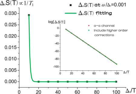
Figure 1: The NMR relaxation rate as a function of temperature. The frequency is chosen to be $\omega/\Delta_{a}=0.001$. The temperature dependence is well described by $\Delta_{a}S(T)=631e^{-\Delta_{a}/T}$. The inset picture shows that channels other than $a-a$ give negligible contributions.

Next, we consider $D_{1,2}+D_{2,1}$, the terms with a one-particle and a two-particle state. Up to the order $\mathcal{O}(e^{-2\Delta_{a}/T})$, we focus on the case when all three particles are the lightest $a$ particle (the other channels $aa-b$ and $aa-c$ are expected to behave similarly), which we find to be supplement ,

$$S_{(1,2)+(2,1)}(\omega,q)=\frac{1}{{\pi}}\int_{-\infty}^{\infty}{\frac{{d\theta e^{-\beta\Delta_{a}\cosh\theta}}}{{\left|{\sqrt{\left({f\tilde{\omega},\tilde{q},\theta)-1}\right)^{2}-1}}\right|}}}\\ \cdot F_{3}^{\sigma}\left({\theta+i\pi,\ln x_{+},\ln x_{-}}\right)F_{3}^{\sigma}\left({\theta+i\pi,\ln x_{-},\ln x_{+}}\right),$$ (24)

where

$$x_{\pm}=\frac{1}{2}(\tilde{\omega}+\cosh\theta+\tilde{q}+\sinh\theta)\left(1\pm 2\sqrt{1-2/f(\tilde{\omega},\tilde{q},\theta)}\right),$$ (25)

and $f(\tilde{\omega},\tilde{q},\theta)=\left[{\left({\tilde{\omega}+\cosh\theta}\right)^{2}-\left({\tilde{q}+\sinh\theta}\right)^{2}}\right]/2$ with $\tilde{\omega}=\omega/\Delta_{a}$ and $\tilde{q}=q/\Delta_{a}.$ Our analysis supplement shows no contributions from the range $\tilde{\omega}>\tilde{q}\geq 0$, where $\cosh\theta\sim 1/\tilde{\omega}\gg 1$. In the range $\tilde{\omega}\leq\tilde{q}$, we have $\cosh\theta\gtrsim 2-\tilde{\omega}$, indicating there exists a small region of $\tilde{q}$ where $\cosh\theta$ is slightly smaller than $2$. This contribution is expected to be small, and we confirm this by including the channels $D_{1,2}+D_{2,1}$ in our numerical calculation shown below.

For connected parts in $D_{2,2}$, a similar Jacobian will appear as in the calculation of the equal mass case of Eq. (S28), and we will encounter the same logarithmic divergence in the frequency dependence. We find no singular terms beyond the logarithmic divergence supplement . This contribution is therefore suppressed by the thermal weight $e^{-2\Delta_{a}/T}$. Low-frequency divergences are also expected to come from the $D_{nn}$ terms (at $n>2$) with particles of the same mass in the two asymptotic states of the form factors. The fact that $D_{22}$ with the same particle does not contain singularities stronger than $\ln\omega$ is a strong indication that none of the higher terms in the series will give a stronger (e.g. power-law) singularity. We conjecture that the $D_{nn}$ terms at $n>2$ have a similar logarithmic singularity in the frequency dependence, and they are then also negligible compared to $D_{11}$ due to the stronger thermal suppression factor.

Numerical analysis.—

Fig. 1 shows the results and fit for the NMR relaxation rate as a function of temperature in the range $\Delta_{a}/T\in[10,100]$ at a fixed low frequency $\omega/\Delta_{a}=0.001$ appropriate for the NMR experiments (satisfying $\omega\ll T$). The fitting function $\Delta_{a}S(T)=631e^{-\Delta_{a}/T}$ indicates that the behavior of relaxation rate at low frequency and low temperature region is dominated by the contribution from the $a-a$ channel, as clearly shown in the inset to Fig. 1. The prefactor 631 compares well with the analytical expression associated with $S_{1,1}$ of the lightest $a$-particle: since $2|F_{2}^{\sigma}(i\pi,0)|_{\Delta_{1}=\Delta_{2}=\Delta_{a}}^{2}\approx 130$.

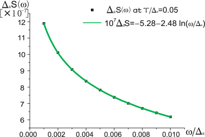
Figure 2: The local dynamical structure factor as a function of frequency at a fixed temperature $T/\Delta_{a}=0.05$. The $\omega$-dependence is well described by $10^{7}\Delta_{a}S(\omega)=-5.28+2.48\ln(\Delta_{a}/\omega)$.

We also study the frequency dependence of the local DSF at fixed temperatures for $T,\omega\ll\Delta_{a}$. Fig. 2 shows the result at a fixed $T/\Delta_{a}=0.05$ with $\omega/\Delta_{a}$ ranging from $0.001$ to $0.01$ (satisfying $\omega\ll T$. It is well fitted as $10^{7}\Delta_{a}S(\omega)=-5.28-2.48\ln(\omega/\Delta_{a})$, which is in accordance with the asymptotic form Eq. (23).

Discussion.—

We conclude that the temperature dependence of the NMR relaxation rate is given by

$$\frac{1}{{T_{1}}}\approx\frac{c^{2}b}{{\Delta_{a}}}\frac{A^{2}}{{2N}}e^{-\Delta_{a}/T};\;\Delta_{a}\approx 4.405\left|h\right|^{8/15}.$$ (26)

In the prefactor, $c\approx 0.783$ is the aforementioned conversion factor between the $\sigma$ field and the lattice spin delfino1 , and $b\approx\ln(4T/\omega_{0})-\gamma_{E}$.

We next consider the implications of our results for CoNb₂O₆. The neutron scattering experiments provided evidence for the two lightest particles of the $E_{8}$ spectrum coldea . This has been understood by considering the effect of the inter-chain coupling in the three-dimensionally ordered state as inducing a longitudinal field coldea ; lee . Further test of the $E_{8}$ description would be provided by measuring the spin dynamics at finite temperatures. Our study here provides a concrete prediction of the temperature-dependence of the NMR relaxation rate in the $E_{8}$ model, which can be used for the desired further test. During the final stage of writing the present manuscript, NMR measurements in CoNb₂O₆ have been reported in the higher-temperature quantum critical regime kinross ; such measurements at the lower-temperature $E_{8}$ regime should therefore be feasible.

To summarize, we have determined the local dynamical spin structure factor of the perturbed quantum-critical Ising chain at temperatures and frequencies that are small compared to the mass of the lightest $E_{8}$ particle. The frequency dependence shows a logarithmic singularity. Our calculation yields a concrete prediction for the temperature dependence of the NMR relaxation rate, which we have suggested as a means to further test the $E_{8}$ description of the spin dynamics in CoNb₂O₆.

I Acknowledgement

We thank R. Coldea, F.H.L.Essler, Gábor Takács and J. H.H. Perk for useful discussions. J.W. and Q.S. acknowledge the support provided in part by the NSF Grant No. DMR-1309531 and the Robert A. Welch Foundation Grant No. C-1411, and M.K. acknowledges that by the Marie Curie IIF Grant PIIF-GA-2012- 330076. Q.S.  also acknowledges the support of the Alexander von Humboldt Foundation, and the hospitality of the the Karlsruhe Institute of Technology and the Institute of Physics of Chinese Academy of Sciences.

Supplementary Material —- Finite temperature spin dynamics
in a perturbed quantum critical Ising chain with an $E_{8}$ symmetry

Jinda Wu, Márton Kormos and Qimiao Si

II Derivation of $\chi_{yy}(x,t)$

The Hamiltonian of one dimensional transverse field Ising model with a longitudinal field can be expressed as

$$H=-J\left({\sum\limits_{i}{\sigma_{i}^{z}\sigma_{i+1}^{z}}+g\sum\limits_{i}{\sigma_{i}^{x}}+h_{z}\sum\limits_{i}{\sigma_{i}^{z}}}\right)$$ (S1)

where $J$, $g$ and $h_{z}$ have the same meaning as in the main text. Consider $C\left({i,j,t,T}\right)=\left\langle{\sigma_{i}^{z}(t)\sigma_{j}^{z}(0)}\right\rangle_{T}$, where $\left\langle\cdots\right\rangle_{T}$ denotes thermal averaging. We have

$$\frac{{\partial C\left({i,j,t,T}\right)}}{{\partial t}}=-Jgi\left\langle{e^{iHt}\left[{\sigma_{i}^{x}(0),\;\sigma_{i}^{z}(0)}\right]e^{-iHt}\sigma_{i}^{z}(0)}\right\rangle=-2Jg\left\langle{\sigma_{i}^{y}(t)\sigma_{j}^{z}(0)}\right\rangle_{T}=-2Jg\left\langle{\sigma_{i}^{y}(0)\sigma_{j}^{z}(-t)}\right\rangle_{T}$$ (S2)

and

$$\frac{{\partial^{2}C\left({i,j,t,T}\right)}}{{\partial t^{2}}}=\left({-Jg}\right)2\frac{{\partial\left\langle{\sigma_{i}^{y}(0)\sigma_{j}^{z}(-t)}\right\rangle_{T}}}{{\partial t}}=\left({-Jg}\right)^{2}(-4)\left\langle{\sigma_{i}^{y}(t)\sigma_{j}^{y}(0)}\right\rangle_{T}=-4\left({Jg}\right)^{2}\left\langle{\sigma_{i}^{y}(t)\sigma_{j}^{y}(0)}\right\rangle_{T}$$ (S3)

Recall the definition of linear response $\chi_{ij,T}^{\alpha\alpha},\alpha=x,y,z$,

$$\chi_{ij,T}^{\alpha\alpha}=-i\theta(t)\left\langle{\left[{\sigma_{i}^{\alpha}(t),\sigma_{j}^{\alpha}(0)}\right]}\right\rangle_{T}$$ (S4)

We have

$$\chi_{T}^{yy}(x,t)=-\frac{1}{{4(gJ)^{2}}}\frac{{\partial^{2}\chi_{T}^{zz}(x,t)}}{{\partial t^{2}}}$$ (S5)

Then

$$\chi_{T}^{yy}(\omega)=\frac{{\omega^{2}}}{{4(gJ)^{2}}}\chi_{T}^{zz}(\omega)$$ (S6)

III Relevant Form Factors used in the Main Text

The main text considered two- and three-particle form factors of the $E_{8}$ model. The relevant two-particle form factors are known in the literaturedelfino1 ; delfino2 . Here, for completeness, we present their detailed expressions, where“$n$” in $F_{n}^{\sigma}$ is explicitly written as types of particles it contains.

$$F_{aa}^{\sigma}\left({\theta_{1},\theta_{2}}\right)=\left\{{c_{11}^{0}+c_{11}^{1}\cosh\left({\theta_{1}-\theta_{2}}\right)}\right\}\left\{{-i\sinh\left({\frac{{\theta_{1}-\theta_{2}}}{2}}\right)}\right\}\frac{{T_{2/3}\left({\theta_{1}-\theta_{2}}\right)T_{2/5}\left({\theta_{1}-\theta_{2}}\right)T_{1/15}\left({\theta_{1}-\theta_{2}}\right)}}{{P_{2/3}\left({\theta_{1}-\theta_{2}}\right)P_{2/5}\left({\theta_{1}-\theta_{2}}\right)P_{1/15}\left({\theta_{1}-\theta_{2}}\right)}}$$ (S7)

$$F_{bb}^{\sigma}\left({\theta_{1},\theta_{2}}\right)=\left\{{c_{22}^{0}+c_{22}^{1}\cosh\left({\theta_{1}-\theta_{2}}\right)+c_{22}^{2}\cosh^{2}\left({\theta_{1}-\theta_{2}}\right)+c_{22}^{3}\cosh^{3}\left({\theta_{1}-\theta_{2}}\right)}\right\}\left\{{-i\sinh\left({\frac{{\theta_{1}-\theta_{2}}}{2}}\right)}\right\}\cdot\;\;$$ (S8)

$$\;\;\;\;\;\;\;\;\;\cdot\frac{{T_{4/5}\left({\theta_{1}-\theta_{2}}\right)T_{2/3}\left({\theta_{1}-\theta_{2}}\right)T_{7/15}\left({\theta_{1}-\theta_{2}}\right)T_{4/15}\left({\theta_{1}-\theta_{2}}\right)T_{1/15}\left({\theta_{1}-\theta_{2}}\right)\left({T_{2/5}\left({\theta_{1}-\theta_{2}}\right)}\right)^{2}}}{{P_{4/5}\left({\theta_{1}-\theta_{2}}\right)P_{2/3}\left({\theta_{1}-\theta_{2}}\right)P_{7/15}\left({\theta_{1}-\theta_{2}}\right)P_{4/15}\left({\theta_{1}-\theta_{2}}\right)P_{1/15}\left({\theta_{1}-\theta_{2}}\right)P_{2/5}\left({\theta_{1}-\theta_{2}}\right)P_{3/5}\left({\theta_{1}-\theta_{2}}\right)}}$$

$$F_{cc}^{\sigma}\left({\theta_{1},\theta_{2}}\right)=\left\{{c_{33}^{0}+c_{33}^{1}\cosh\left({\theta_{1}-\theta_{2}}\right)+c_{33}^{2}\cosh^{2}\left({\theta_{1}-\theta_{2}}\right)+c_{33}^{3}\cosh^{3}\left({\theta_{1}-\theta_{2}}\right)+c_{33}^{4}\cosh^{4}\left({\theta_{1}-\theta_{2}}\right)}\right\}\cdot$$

$$\cdot\left\{{-i\sinh\left({\frac{{\theta_{1}-\theta_{2}}}{2}}\right)}\right\}T_{11/30}\left({\theta_{1}-\theta_{2}}\right)\left[{T_{2/3}\left({\theta_{1}-\theta_{2}}\right)}\right]^{3}T_{7/15}\left({\theta_{1}-\theta_{2}}\right)\left[{T_{2/5}\left({\theta_{1}-\theta_{2}}\right)}\right]^{3}T_{2/15}\left({\theta_{1}-\theta_{2}}\right)\cdot$$

$$\cdot\left[{T_{1/15}\left({\theta_{1}-\theta_{2}}\right)}\right]^{2}/\left\{{P_{11/30}\left({\theta_{1}-\theta_{2}}\right)P_{7/15}\left({\theta_{1}-\theta_{2}}\right)P_{2/15}\left({\theta_{1}-\theta_{2}}\right)\left[{P_{2/3}\left({\theta_{1}-\theta_{2}}\right)}\right]^{2}P_{1/3}\left({\theta_{1}-\theta_{2}}\right)\cdot}\right.$$

$$\left.{\cdot\left[{P_{2/5}\left({\theta_{1}-\theta_{2}}\right)}\right]^{2}P_{3/5}\left({\theta_{1}-\theta_{2}}\right)P_{1/15}\left({\theta_{1}-\theta_{2}}\right)P_{14/15}\left({\theta_{1}-\theta_{2}}\right)}\right\}$$ (S9)

$$F_{ab}^{\sigma}\left({\theta_{1},\theta_{2}}\right) = \left\{{c_{12}^{0}+c_{12}^{1}\cosh\left({\theta_{1}-\theta_{2}}\right)+c_{12}^{2}\cosh^{2}\left({\theta_{1}-\theta_{2}}\right)}\right\}\frac{{T_{4/5}\left({\theta_{1}-\theta_{2}}\right)T_{3/5}\left({\theta_{1}-\theta_{2}}\right)T_{7/15}\left({\theta_{1}-\theta_{2}}\right)T_{4/15}\left({\theta_{1}-\theta_{2}}\right)}}{{P_{4/5}\left({\theta_{1}-\theta_{2}}\right)P_{3/5}\left({\theta_{1}-\theta_{2}}\right)P_{7/15}\left({\theta_{1}-\theta_{2}}\right)P_{4/15}\left({\theta_{1}-\theta_{2}}\right)}}$$

$$F_{ac}^{\sigma}\left({\theta_{1},\theta_{2}}\right) = \left\{{c_{13}^{0}+c_{13}^{1}\cosh\left({\theta_{1}-\theta_{2}}\right)+c_{13}^{2}\cosh^{2}\left({\theta_{1}-\theta_{2}}\right)+c_{13}^{3}\cosh^{3}\left({\theta_{1}-\theta_{2}}\right)}\right\}\cdot$$ (S11)

$$\cdot\frac{{T_{29/30}\left({\theta_{1}-\theta_{2}}\right)T_{7/10}\left({\theta_{1}-\theta_{2}}\right)T_{13/30}\left({\theta_{1}-\theta_{2}}\right)T_{1/10}\left({\theta_{1}-\theta_{2}}\right)\left[{T_{11/30}\left({\theta_{1}-\theta_{2}}\right)}\right]^{2}}}{{P_{29/30}\left({\theta_{1}-\theta_{2}}\right)P_{7/10}\left({\theta_{1}-\theta_{2}}\right)P_{13/30}\left({\theta_{1}-\theta_{2}}\right)P_{1/10}\left({\theta_{1}-\theta_{2}}\right)P_{11/30}\left({\theta_{1}-\theta_{2}}\right)P_{19/30}\left({\theta_{1}-\theta_{2}}\right)}}$$

$$F_{bc}^{\sigma}\left({\theta_{1},\theta_{2}}\right) = \left\{{c_{23}^{0}+c_{23}^{1}\cosh\left({\theta_{1}-\theta_{2}}\right)+c_{23}^{2}\cosh^{2}\left({\theta_{1}-\theta_{2}}\right)+c_{23}^{3}\cosh^{3}\left({\theta_{1}-\theta_{2}}\right)+c_{23}^{4}\cosh^{4}\left({\theta_{1}-\theta_{2}}\right)}\right\}\cdot$$

$$\frac{{T_{25/30}\left({\theta_{1}-\theta_{2}}\right)T_{19/30}\left({\theta_{1}-\theta_{2}}\right)T_{9/30}\left({\theta_{1}-\theta_{2}}\right)\left[{T_{7/30}\left({\theta_{1}-\theta_{2}}\right)}\right]^{2}\left[{T_{13/30}\left({\theta_{1}-\theta_{2}}\right)}\right]^{2}T_{15/30}\left({\theta_{1}-\theta_{2}}\right)}}{{P_{25/30}\left({\theta_{1}-\theta_{2}}\right)P_{19/30}\left({\theta_{1}-\theta_{2}}\right)P_{9/30}\left({\theta_{1}-\theta_{2}}\right)P_{7/30}\left({\theta_{1}-\theta_{2}}\right)P_{23/30}\left({\theta_{1}-\theta_{2}}\right)P_{13/30}\left({\theta_{1}-\theta_{2}}\right)P_{17/30}\left({\theta_{1}-\theta_{2}}\right)P_{15/30}\left({\theta_{1}-\theta_{2}}\right)}}$$ (S12)

where

$$T_{\lambda}(\theta)=\exp\left\{{2\int_{0}^{\infty}{\frac{{dt}}{t}\frac{{\cosh\left[{\left({\lambda-1/2}\right)t}\right]}}{{\cosh\left({t/2}\right)\sinh t}}\sin^{2}\frac{{\left({i\pi-\theta}\right)t}}{{2\pi}}}}\right\}\;\;and\;\;P_{\lambda}(\theta)=\frac{{\cos\left({\lambda\pi}\right)-\cosh\theta}}{{2\cos^{2}\left({\lambda\pi/2}\right)}}.$$ (S13)

The coefficients $\{c_{ij}^{k}\}$ in the above expressions are delfino2 :

$$\begin{array}[]{l}c_{11}^{0},c_{11}^{1}=-10.19307727,-2.09310293\\ c_{22}^{0},c_{22}^{1},c_{22}^{2},c_{22}^{3}=-500.2535896,-791.3745549,-338.8125724,-21.48559881\\ c_{33}^{0},c_{33}^{1},c_{33}^{2},c_{33}^{3},c_{33}^{4},c_{33}^{5}=-87821.70785,-267341.1276,-301093.9432,-150512.4122,-30166.99117,-1197.056497\\ c_{12}^{0},c_{12}^{1},c_{12}^{2}=-{\rm{70}}{\rm{.29218939519}},-{\rm{71}}{\rm{.792063506}},-{\rm{7}}{\rm{.9790221816}}\\ c_{13}^{0},c_{13}^{1},c_{13}^{2},c_{13}^{3}=-{\rm{7049}}{\rm{.622303}},-{\rm{13406}}{\rm{.48877}},-{\rm{6944}}{\rm{.416956}},-{\rm{582}}{\rm{.2557366}}\\ c_{23}^{0},c_{23}^{1},c_{23}^{2},c_{23}^{3},c_{23}^{4}=-{\rm{3579}}{\rm{.556465}},-{\rm{8436}}{\rm{.850081}},-{\rm{6618}}{\rm{.297073}},-{\rm{1846}}{\rm{.579035}},-{\rm{92}}{\rm{.73452314}}\\ \end{array}$$

The relevant three-particle form factor of the $E_{8}$ model is,

$$F_{aaa}^{\sigma}\left({\theta_{1},\theta_{2},\theta_{3}}\right)=Q_{aaa}^{\sigma}\left({\theta_{1},\theta_{2},\theta_{3}}\right)\frac{{F_{aa}^{\min}\left({\theta_{1}-\theta_{2}}\right)}}{{\left({e^{\theta_{1}}+e^{\theta_{2}}}\right)D_{aa}\left({\theta_{1}-\theta_{2}}\right)}}\frac{{F_{aa}^{\min}\left({\theta_{1}-\theta_{3}}\right)}}{{\left({e^{\theta_{1}}+e^{\theta_{3}}}\right)D_{aa}\left({\theta_{1}-\theta_{3}}\right)}}\frac{{F_{aa}^{\min}\left({\theta_{2}-\theta_{3}}\right)}}{{\left({e^{\theta_{2}}+e^{\theta_{3}}}\right)D_{aa}\left({\theta_{2}-\theta_{3}}\right)}}$$ (S14)

wheredelfino1 ; delfino2

$$\frac{{F_{aa}^{\min}\left({\theta_{i}-\theta_{j}}\right)}}{{D_{aa}\left({\theta_{i}-\theta_{j}}\right)}}=\left\{{-i\sinh\left({\frac{{\theta_{i}-\theta_{j}}}{2}}\right)}\right\}\frac{{T_{2/3}\left({\theta_{i}-\theta_{j}}\right)T_{2/5}\left({\theta_{i}-\theta_{j}}\right)T_{1/15}\left({\theta_{i}-\theta_{j}}\right)}}{{P_{2/3}\left({\theta_{i}-\theta_{j}}\right)P_{2/5}\left({\theta_{i}-\theta_{j}}\right)P_{1/15}\left({\theta_{i}-\theta_{j}}\right)}}$$ (S15)

anddelfino3

$$Q_{aaa}^{\sigma}\left({\theta_{1},\theta_{2},\theta_{3}}\right)=1148.690509{\rm{}}e^{3\theta_{1}}+46.76252978{\rm{}}e^{4\theta_{1}-\theta_{2}}+1148.690509{\rm{}}e^{3\theta_{2}}+3703.911733{\rm{}}e^{2\theta_{1}+\theta_{2}}$$

$$+3703.911733{\rm{}}e^{\theta_{1}+2\theta_{2}}+46.76252978{\rm{}}e^{-\theta_{1}+4\theta_{2}}+4.354182251{\rm{}}e^{4\theta_{1}+\theta_{2}-2\theta_{3}}+46.76252978{\rm{}}e^{3\theta_{1}+2\theta_{2}-2\theta_{3}}$$

$$+46.76252978{\rm{}}e^{2\theta_{1}+3\theta_{2}-2\theta_{3}}+4.354182251{\rm{}}e^{\theta_{1}+4\theta_{2}-2\theta_{3}}+46.76252978{\rm{}}e^{4\theta_{1}-\theta_{3}}+604.2577928{\rm{}}e^{3\theta_{1}+\theta_{2}-\theta_{3}}$$

$$+1148.690509{\rm{}}e^{2\theta_{1}+2\theta_{2}-\theta_{3}}+604.2577928\;e^{\theta_{1}+3\theta_{2}-\theta_{3}}+46.76252978{\rm{}}e^{4\theta_{2}-\theta_{3}}+1148.690509{\rm{}}e^{3\theta_{3}}$$

$$+3703.911733{\rm{}}e^{2\theta_{1}+\theta_{3}}+4.354182251{\rm{}}e^{4\theta_{1}-2\theta_{2}+\theta_{3}}+604.2577928{\rm{}}e^{3\theta_{1}-\theta_{2}+\theta_{3}}+6286.815608\;e^{\theta_{1}+\theta_{2}+\theta_{3}}$$

$$+3703.911733{\rm{}}e^{2\theta_{2}+\theta_{3}}+604.2577928\;e^{-\theta_{1}+3\theta_{2}+\theta_{3}}+4.354182251{\rm{}}e^{-2\theta_{1}+4\theta_{2}+\theta_{3}}+3703.911733{\rm{}}e^{\theta_{1}+2\theta_{3}}$$

$$+46.76252978{\rm{}}e^{3\theta_{1}-2\theta_{2}+2\theta_{3}}+1148.690509{\rm{}}e^{2\theta_{1}-\theta_{2}+2\theta_{3}}+3703.911733{\rm{}}e^{\theta_{2}+2\theta_{3}}+1148.690509{\rm{}}e^{-\theta_{1}+2\theta_{2}+2\theta_{3}}$$

$$+46.76252978{\rm{}}e^{-2\theta_{1}+3\theta_{2}+2\theta_{3}}+46.76252978{\rm{}}e^{2\theta_{1}-2\theta_{2}+3\theta_{3}}+604.2577928{\rm{}}e^{\theta_{1}-\theta_{2}+3\theta_{3}}+604.2577928{\rm{}}e^{-\theta_{1}+\theta_{2}+3\theta_{3}}$$

$$+46.76252978{\rm{}}e^{-2\theta_{1}+2\theta_{2}+3\theta_{3}}+46.76252978{\rm{}}e^{-\theta_{1}+4\theta_{3}}+4.354182251{\rm{}}e^{\theta_{1}-2\theta_{2}+4\theta_{3}}+46.76252978{\rm{}}e^{-\theta_{2}+4\theta_{3}}$$

$$+4.354182251{\rm{}}e^{-2\theta_{1}+\theta_{2}+4\theta_{3}}$$ (S16)

IV Derivation of $S_{1,1}(\omega,q)$ (Eq.(19) of the Main Text)

We calculate $S_{1,1}$ using the finite volume regularization scheme pozsgay ; szecsenyi . We have $D_{00}=\left\langle\sigma\right\rangle_{0}^{2}$, and

$$\begin{gathered}D_{11}(x,t)=\int_{-\infty}^{\infty}{\frac{{d\theta_{1}}}{{2\pi}}\int_{-\infty}^{\infty}{\frac{{d\theta^{\prime}_{1}}}{{2\pi}}F_{2}^{\sigma}\left({\theta_{1}+i\pi,\theta^{\prime}_{1}}\right)F_{2}^{\sigma}\left({\theta^{\prime}_{1}+i\pi,\theta_{1}}\right)}}\cdot\\ \cdot e^{-\beta\Delta_{1}\cosh\theta_{1}}e^{-i\left({\Delta_{1}\sinh\theta_{1}-\Delta_{2}\sinh\theta^{\prime}_{1}}\right)x}e^{-i\left({\Delta_{2}\cosh\theta^{\prime}_{1}-\Delta_{1}\cosh\theta_{1}}\right)t}+2\left\langle\sigma\right\rangle_{0}F_{2s}^{\sigma}\int_{-\infty}^{\infty}{\frac{{d\theta}}{{2\pi}}e^{-\beta\Delta_{1}\cosh\theta_{1}}}\\ \end{gathered}$$ (S17)

From now until the calculation of $D_{22}$, we will focus on the time-dependent parts, i.e., the connected pieces of the correlation functions. The time-independent parts, i.e., the disconnected pieces, will be discussed after the analysis on the time-dependent parts of $D_{22}$. We then have

$$\begin{gathered}S_{1,1}(q,\omega)=\int{d\theta_{1}d\theta^{\prime}_{1}F_{2}^{\sigma}(\theta_{1}+i\pi,\theta^{\prime}_{1})F_{2}^{\sigma}(\theta^{\prime}_{1}+i\pi,\theta_{1})e^{-\beta\Delta_{1}\cosh\theta_{1}}\cdot}\;\;\;\;\;\;\;\;\;\;\;\;\;\;\;\;\;\;\;\;\;\;\;\;\;\;\;\;\;\;\;\;\;\;\;\;\\ \cdot\delta(q+\Delta_{1}\sinh\theta_{1}-\Delta_{2}\sinh\theta^{\prime}_{1})\delta(\omega+\Delta_{1}\cosh\theta_{1}-\Delta_{2}\cosh\theta^{\prime}_{1})\\ \end{gathered}$$ (S18)

Denote

$$\left\{\begin{array}[]{l}y=\Delta_{1}\sinh\theta_{1}-\Delta_{2}\sinh\theta^{\prime}_{1}\\ z=\Delta_{1}\cosh\theta_{1}-\Delta_{2}\cosh\theta^{\prime}_{1}\\ \end{array}\right.$$ (S19)

then

$$d\theta_{1}d\theta^{\prime}_{1}=\left|{\frac{{\partial\left({\theta_{1},\theta^{\prime}_{1}}\right)}}{{\partial\left({y,z}\right)}}}\right|dydz=\frac{{dydz}}{{\Delta_{1}\Delta_{2}|\sinh\alpha|}},$$ (S20)

where

$$\alpha={\rm{arccosh}}\left[\frac{{\Delta_{1}^{2}+\Delta_{2}^{2}-\left({\omega^{2}-q^{2}}\right)}}{{2\Delta_{1}\Delta_{2}}}\right].$$ (S21)

Noticing that the integration ranges for new variables $y$ and $z$ run from $-\infty$ to $+\infty$, we can easily perform the integral in the structure factor and find

$$S_{1,1}(q,\omega)=\int{d\theta_{1}d\theta^{\prime}_{1}F_{2}^{\sigma}(\theta_{1}+i\pi,\theta^{\prime}_{1})F_{2}^{\sigma}(\theta^{\prime}_{1}+i\pi,\theta_{1})\delta(q+\Delta_{1}\sinh\theta_{1}-\Delta_{2}\sinh\theta^{\prime}_{1})}\cdot$$ (S22)

$$\;\;\;\;\;\;\;\;\;\;\;\;\;\;\;\;\;\;\;\;\;\;\;\;\;\;\;\;\;\;\;\;\;\;\;\;\;\;\;\;\;\;\;\;\;\;\;\;\;\;\;\;\;\;\;\;\;\;\;\;\;\;\;\;\;\;\;\cdot\delta(\omega+\Delta_{1}\cosh\theta_{1}-\Delta_{2}\cosh\theta^{\prime}_{1})e^{-\beta\Delta_{1}\cosh\theta_{1}}$$

$$= \left.{\frac{{F_{2}^{\sigma}(\theta_{1}+i\pi,\theta^{\prime}_{1})F_{2}^{\sigma}(\theta^{\prime}_{1}+i\pi,\theta_{1})e^{-\beta\Delta_{2}\cosh\theta^{\prime}_{1}}e^{\beta\omega}}}{{\Delta_{1}\Delta_{2}|\sinh\alpha|}}}\right|_{\theta_{1}-\theta^{\prime}_{1}=\alpha}+\left.{\frac{{F_{2}^{\sigma}(\theta_{1}+i\pi,\theta^{\prime}_{1})F_{2}^{\sigma}(\theta^{\prime}_{1}+i\pi,\theta_{1})e^{-\beta\Delta_{2}\cosh\theta^{\prime}_{1}}e^{\beta\omega}}}{{\Delta_{1}\Delta_{2}|\sinh\alpha|}}}\right|_{\theta_{1}-\theta^{\prime}_{1}=-\alpha}$$ (S23)

$$= \frac{{\left|{F_{2}^{\sigma}(\alpha+i\pi,0)}\right|^{2}e^{-\beta\Delta_{1}\cosh\theta_{1_{+}}}}}{{\Delta_{1}\Delta_{2}|\sinh\alpha|}}+\frac{{\left|{F_{2}^{\sigma}(-\alpha+i\pi,0)}\right|^{2}e^{-\beta\Delta_{1}\cosh\theta_{1_{-}}}}}{{\Delta_{1}\Delta_{2}|\sinh\alpha|}}$$ (S24)

$$= \frac{{\left|{F_{2}^{\sigma}(\alpha+i\pi,0)}\right|^{2}\left(e^{-\beta\Delta_{1}\cosh\theta_{1_{+}}}+e^{-\beta\Delta_{1}\cosh\theta_{1_{-}}}\right)}}{{\Delta_{1}\Delta_{2}|\sinh\alpha|}}$$ (S25)

where

$$\cosh\theta_{1_{\pm}}=\frac{{\omega\Delta_{1}-\omega\Delta_{2}\Gamma\pm q\Delta_{2}\sqrt{\Gamma^{2}-1}}}{{q^{2}-\omega^{2}}}$$ (S26)

In going from Eq. (S23) to Eq. (S24), we have used the fact that the form factor is only dependent on the difference between any two rapidities. We then recover Eq.(19) of the main text.

V Calculation of $S_{1,1}(\omega,q)$ (Eq.(21) of the Main Text) for Equal Masses at Low Frequencies

In Eq. (S22) above, the $q$ integration followed by the $\theta^{\prime}_{1}$ integration gives rise to

$$S_{1,1}(\omega)=\frac{2}{{\Delta_{i}}}\int{d\theta_{1}\frac{{\left({|F_{2}^{\sigma}(\theta_{1}-\theta^{\prime}_{1+}(\theta_{1},\omega)+i\pi,0)|^{2}+|F_{2}^{\sigma}(\theta_{1}-\theta^{\prime}_{1-}(\theta_{1},\omega)+i\pi,0)|^{2}}\right)e^{-\beta\Delta_{i}\cosh\theta_{1}}}}{{\sqrt{\left({\cosh\theta_{1}+\omega/\Delta_{i}}\right)^{2}-1}}}}$$ (S27)

where $\theta^{\prime}_{1\pm}=\pm{\text{arccosh}}\left({\cosh\theta_{1}+\omega/\Delta_{i}}\right)$. We make a further variable transform $\cosh\theta_{1}=x-\omega_{i}$ ($\omega_{i}=\omega/(2\Delta_{i})$) and have

$$\left.{S_{1,1}(\omega_{i})}\right|_{\Delta_{1}=\Delta_{2}=\Delta_{i}}=\frac{{2e^{\omega/(2T)}}}{\Delta_{i}}\int_{1+\omega_{i}}^{\infty}{dx\frac{{(F\left({\omega_{i},q_{-}(x)}\right)+F\left({\omega_{i},q_{+}(x)}\right))\exp\left\{{-\frac{{\Delta_{i}}}{T}x}\right\}}}{{\sqrt{\left({x+1+\omega_{i}}\right)\left({x+1-\omega_{i}}\right)\left({x-1+\omega_{i}}\right)\left({x-1-\omega_{i}}\right)}}}}$$ (S28)

where $\omega_{i}=\omega/(2\Delta_{i})$, and

$$F(\omega_{i},q_{\pm}(x))=\left|{F_{ii}^{\sigma}({\rm{arccosh}}\left[{{\rm{1+}}\left({-\omega_{i}^{2}+x^{2}-1\pm\sqrt{\left({x-1-\omega_{i}}\right)\left({x-1+\omega_{i}}\right)\left({x+1+\omega_{i}}\right)\left({x+1-\omega_{i}}\right)}}\right)}\right]+i\pi,0)}\right|^{2}$$ (S29)

We can also get Eq. (S28) by making variable transform $x=-\omega/(2\Delta_{i})+\left[{q/\left({2\Delta_{i}}\right)}\right]\sqrt{\left({q^{2}-\omega^{2}+4\Delta_{i}^{2}}\right)/\left({q^{2}-\omega^{2}}\right)}$ for the $q$ integration over Eq. (S25). The exponential-decaying factor in the integrand of Eq. (S28) indicates that the dominant contribution come from the regime where $x$ is close to $1+\omega_{i}$. Since $\omega_{i}$ is small, in this regime we can approximate $F(\omega_{i},q_{\pm}(x))$ as

$$F(\omega_{i},q_{\pm}(x))\approx|F_{ii}^{\sigma}(i\pi,0)|^{2}\;\;(i=a,b,c,d,e,f,g,h).$$ (S30)

Then we have

$$\left.{S_{1,1}(\omega\to 0,\omega/\Delta_{i}\ll 1)}\right|_{\Delta_{1}=\Delta_{2}=\Delta_{i}}$$ (S31)

$$\approx \frac{{4e^{\omega/(2T)}}}{\Delta_{i}}\int_{1+\omega_{i}}^{\infty}{dx\frac{{\left|{F_{ii}\left({i\pi,0}\right)}\right|^{2}\exp\left\{{-\frac{{\Delta_{i}}}{T}x}\right\}}}{{\sqrt{\left({x+1+\omega_{i}}\right)\left({x+1-\omega_{i}}\right)\left({x-1+\omega_{i}}\right)\left({x-1-\omega_{i}}\right)}}}}$$ (S32)

$$\approx \left\{\begin{array}[]{l}\frac{{2e^{\omega/(2T)}\left|{F_{ii}\left({i\pi,0}\right)}\right|^{2}}}{\Delta_{i}}e^{-\Delta_{i}/T}\left\{{-\ln\frac{\omega}{{4T}}-\gamma_{E}+\cdots\cdots}\right\}\;(\omega\ll T\ll\Delta_{i})\\ \frac{{2e^{-\Delta_{i}/T}\left|{F_{ii}\left({i\pi}\right)}\right|^{2}}}{{\Delta_{i}}}\left\{{\sqrt{\frac{{\pi T}}{\omega}}-\frac{{\sqrt{\pi}}}{4}\left({\frac{T}{\omega}}\right)^{3/2}+\cdots\cdots}\right\}\;(T\ll\omega\ll\Delta_{i})\\ \end{array}\right.$$ (S35)

where $\left|{F_{aa}^{\sigma}\left({i\pi,0}\right)}\right|^{2}\approx 65$.

VI Derivation of $S_{1,2}(\omega,q)$ (Eq.(22) of the Main Text)

We again use the finite volume regularization scheme pozsgay ; szecsenyi , and have

$$D_{12}(x,t)=C_{12}-Z_{1}C_{01}$$ (S36)

$$= \frac{1}{2}\int_{C_{+}}{\frac{{d\theta_{1}}}{{2\pi}}\int_{-\infty}^{\infty}{\frac{{d\theta^{\prime}_{1}}}{{2\pi}}\int_{-\infty}^{\infty}{\frac{{d\theta^{\prime}_{2}}}{{2\pi}}F_{3}^{\sigma}\left({\theta_{1}+i\pi,\theta^{\prime}_{1},\theta^{\prime}_{2}}\right)F_{3}^{\sigma}\left({\theta_{1}+i\pi,\theta^{\prime}_{2},\theta^{\prime}_{1}}\right)}}}$$ (S42)

$$\;\;\;\;\;\;\;\;\;\;\;\;\;\;\;\;\;\;\;\;\;\;\;\;\;\;\;\;\;\;\;\;\;\;\;\;\;\;\;\;\;\;e^{-\beta\Delta_{a}\cosh\theta_{1}}e^{-ix\Delta_{a}\left({\sinh\theta_{1}-\sinh\theta^{\prime}_{1}-\sinh\theta^{\prime}_{2}}\right)}e^{-it\Delta_{a}\left({\cosh\theta^{\prime}_{1}+\cosh\theta^{\prime}_{2}-\cosh\theta_{1}}\right)}$$

$$+\int_{-\infty}^{\infty}{\frac{{d\theta^{\prime}_{1}}}{{2\pi}}\int_{-\infty}^{\infty}{\frac{{d\theta^{\prime}_{2}}}{{2\pi}}\left\{{e^{-\beta\Delta_{a}\cosh\theta^{\prime}_{1}}e^{i\Delta_{a}x\sinh\theta^{\prime}_{2}}e^{-it\Delta_{a}\cosh\theta^{\prime}_{2}}S\left({\theta^{\prime}_{2}-\theta^{\prime}_{1}}\right)F_{1}^{\sigma}F_{3c}^{\sigma}\left({\theta^{\prime}_{1}|\theta^{\prime}_{1}\theta^{\prime}_{2}}\right)+\left({\theta^{\prime}_{1}\leftrightarrow\theta^{\prime}_{2}}\right)}\right\}}}$$

$$-\left({F_{1}^{\sigma}}\right)^{2}\int_{-\infty}^{\infty}{\frac{{d\theta^{\prime}_{1}}}{{2\pi}}\int_{-\infty}^{\infty}{\frac{{d\theta^{\prime}_{2}}}{{2\pi}}e^{-\beta\Delta_{a}\cosh\theta^{\prime}_{1}}e^{i\Delta_{a}x\sinh\theta^{\prime}_{2}}e^{-it\Delta_{a}\cosh\theta^{\prime}_{2}}\cdot}}$$

$$\;\;\;\;\;\;\;\;\;\;\;\;\;\;\;\;\;\;\;\;\;\;\;\;\;\;\;\;\;\;\;\;\;\;\;\;\;\;\;\;\left({\Delta_{a}x\cosh\theta^{\prime}_{1}+\Delta_{a}\left({i\beta+t}\right)\sinh\theta^{\prime}_{1}}\right)\left[{S\left({\theta^{\prime}_{1}-\theta^{\prime}_{2}}\right)-1}\right]$$

$$-\left({F_{1}^{\sigma}}\right)^{2}\int_{-\infty}^{\infty}{\frac{{d\theta^{\prime}_{2}}}{{2\pi}}e^{-\beta\Delta_{a}\cosh\theta^{\prime}_{2}}e^{i\Delta_{a}x\sinh\theta^{\prime}_{2}}e^{-it\Delta_{a}\cosh\theta^{\prime}_{2}}}$$

where $C_{+}$ is used to denote the integration contour from $-\infty$ to $\infty$ slightly above the real axis on the rapidity complex plane, andpozsgay ; szecsenyi

$$F_{3}^{\sigma}(\theta_{1}+i\pi,\theta^{\prime}_{1},\theta^{\prime}_{2})=\frac{{i\left({1-S(\theta^{\prime}_{1}-\theta^{\prime}_{2})}\right)F_{1}^{\sigma}}}{{\theta_{1}-\theta^{\prime}_{1}}}+\frac{{i\left({S(\theta^{\prime}_{1}-\theta^{\prime}_{2})-1}\right)F_{1}^{\sigma}}}{{\theta_{1}-\theta^{\prime}_{2}}}+F_{3rc}^{\sigma}\left({\theta_{1}+i\pi|\theta^{\prime}_{1},\theta_{2}}\right)$$ (S43)

where $S_{aa}$ is the scattering matrix for $a-a$ channel, and $F_{3rc}^{\sigma}\left({\theta_{1}+i\pi|\theta^{\prime}_{1},\theta_{2}}\right)$ is regular on real axis.

For $x=0$, it’s easy to see that the last three terms do not contribute to low-frequency ($\omega\ll\Delta_{a}$) response of local DSF. Fom the first integration we have

$$S_{1,2}(q,\omega) = \frac{1}{2}\int{\frac{{d\theta_{1}}}{{2\pi}}\int_{-\infty}^{\infty}{d\theta^{\prime}_{1}\int_{-\infty}^{\infty}{d\theta^{\prime}_{2}F_{3}^{\sigma}\left({\theta_{1}+i\pi+i\varepsilon,\theta^{\prime}_{1},\theta^{\prime}_{2}}\right)F_{3}^{\sigma}\left({\theta_{1}+i\pi+i\varepsilon,\theta^{\prime}_{2},\theta^{\prime}_{1}}\right)}}}$$ (S45)

$$\delta\left({q+\Delta_{a}\sinh\theta_{1}-\Delta_{a}\left({\sinh\theta^{\prime}_{1}+\sinh\theta^{\prime}_{2}}\right)}\right)\delta\left({\omega+\Delta_{a}\cosh\theta_{1}-\Delta_{a}\left({\cosh\theta^{\prime}_{1}+\cosh\theta^{\prime}_{2}}\right)}\right)$$

The energy-momentum conservation yields

$$\left\{\begin{array}[]{l}0=q+\sinh\theta_{1}-\sinh\theta^{\prime}_{1}-\sinh\theta^{\prime}_{2}\\ 0=\omega+\cosh\theta_{1}-\cosh\theta^{\prime}_{1}-\cosh\theta^{\prime}_{2}\\ \end{array}\right.$$ (S46)

For $F_{3rc}^{\sigma}$ we can integrate over $\theta^{\prime}_{1}$ and $\theta^{\prime}_{2}$, yielding (because the masses of three particles are equal to each other, $S_{21}(q,\omega)=S_{12}(q,\omega)$)

$$S_{(1,2)+(2,1)}(q,\omega)=\frac{1}{{2\pi}}\int_{-\infty}^{\infty}{\frac{{d\theta_{1}}}{{\left|{\sqrt{\left({f(\tilde{\omega},\tilde{q},\theta_{1})-1}\right)^{2}-1}}\right|}}F_{3rc}^{\sigma}\left({\theta_{1}+i\pi|\ln z_{+},\ln z_{-}}\right)F_{3rc}^{\sigma}\left({\theta_{1}+i\pi|\ln z_{-},\ln z_{+}}\right)e^{-\beta\Delta_{a}\cosh\theta_{1}}}$$ (S47)

with

$$z_{\pm}=\frac{1}{2}(\tilde{\omega}+\cosh\theta+\tilde{q}+\sinh\theta)\left(1\pm 2\sqrt{1-2/f(\tilde{\omega},\tilde{q},\theta)}\right),$$ (S48)

and

$$f(\tilde{\omega},\tilde{q},\theta)=\left[{\left({\tilde{\omega}+\cosh\theta}\right)^{2}-\left({\tilde{q}+\sinh\theta}\right)^{2}}\right]/2$$ (S49)

where $\tilde{\omega}=\omega/\Delta_{a}$ and $\tilde{q}=q/\Delta_{a}$. Thus we recover Eq. (22) of the main text. The energy-momentum conservation gives a constraint: $f(\tilde{\omega},\tilde{q},\theta)\geqslant 2$, i.e., $(\tilde{\omega}-\tilde{q})e^{2\theta}+(\tilde{\omega}^{2}-\tilde{q}^{2}-3)e^{\theta}+\tilde{\omega}+\tilde{q}\geq 0$. This constraint allows zero in the denominator of the integrand in Eq. (S47), which is a branch point. This can be clearly shown after a variable transform $e^{\theta}\to x$ and expanding $x$ around zero. Thus the integration will smooth out the superficial singularity leaving us with a regular integration over $\theta$. Furthermore, if $\tilde{\omega}>\tilde{q}\geq 0$, we can get the constraint for rapidity $0<2e^{\theta}<-\frac{{\tilde{\omega}^{2}-\tilde{q}^{2}-3}}{{\tilde{\omega}-\tilde{q}}}-\sqrt{\left({\frac{{\tilde{\omega}^{2}-\tilde{q}^{2}-3}}{{\tilde{\omega}-\tilde{q}}}}\right)^{2}-4\frac{{\tilde{\omega}+\tilde{q}}}{{\tilde{\omega}-\tilde{q}}}}$ or $2e^{\theta}>-\frac{{\tilde{\omega}^{2}-\tilde{q}^{2}-3}}{{\tilde{\omega}-\tilde{q}}}+\sqrt{\left({\frac{{\tilde{\omega}^{2}-\tilde{q}^{2}-3}}{{\tilde{\omega}-\tilde{q}}}}\right)^{2}-4\frac{{\tilde{\omega}+\tilde{q}}}{{\tilde{\omega}-\tilde{q}}}}$. However, it’s easy to see in these two ranges that, because $\tilde{\omega}\ll 1$, we will have $\cosh\theta\sim 1/\tilde{\omega}$, making it negligible in the zero frequency limit. If $\tilde{\omega}\leq\tilde{q}$, we get constraint on the rapidity of $\theta$ as (without loss of generality we choose $\tilde{\omega}>0$): $0<2e^{\theta}<\left[\left({\tilde{\omega}^{2}-\tilde{q}^{2}-3}\right)+\sqrt{\left({\tilde{\omega}^{2}-\tilde{q}^{2}-1}\right)\left({\tilde{\omega}^{2}-\tilde{q}^{2}-9}\right)}\right]/(\tilde{q}-\tilde{\omega})\equiv\mu(\tilde{\omega},\tilde{q})$. We can then determine the maximum of $\mu(\tilde{\omega},\tilde{q})$ to be located at $\tilde{q}_{m}=\sqrt{(3-\tilde{\omega})(1-\tilde{\omega})}$. Again recalling $\tilde{\omega}\ll 1$, we have $\cosh\theta\gtrsim 2-\tilde{\omega}$. This indicates that a small region of $\tilde{q}$ exists, in which $\cosh\theta$ is slightly smaller than $2$. Therefore, we will include in our numerical calculation the channels $D_{1,2}+D_{2,1}$.

For the leftover two parts in Eq. (S43), we have

$$\frac{{i\left({1-S(\theta^{\prime}_{1}-\theta^{\prime}_{2})}\right)F_{1}^{\sigma}}}{{\theta_{1}-\theta^{\prime}_{1}+i\varepsilon}}=P\frac{{i\left({1-S(\theta^{\prime}_{1}-\theta^{\prime}_{2})}\right)F_{1}^{\sigma}}}{{\theta_{1}-\theta^{\prime}_{1}}}-i\pi\delta(\theta_{1}-\theta^{\prime}_{1}),\hfill$$ (S50)

$$\frac{{i\left({S(\theta^{\prime}_{1}-\theta^{\prime}_{2})-1}\right)F_{1}^{\sigma}}}{{\theta_{1}-\theta^{\prime}_{2}+i\varepsilon}}=P\frac{{i\left({S(\theta^{\prime}_{1}-\theta^{\prime}_{2})-1}\right)F_{1}^{\sigma}}}{{\theta_{1}-\theta^{\prime}_{2}}}-i\pi\delta(\theta_{1}-\theta^{\prime}_{2}).\hfill$$ (S51)

Here $P$ denotes principal value integration. The parts of $F_{3}^{\sigma}\left({\theta_{1}+i\pi+i\varepsilon,\theta^{\prime}_{1},\theta^{\prime}_{2}}\right)F_{3}^{\sigma}\left({\theta_{1}+i\pi+i\varepsilon,\theta^{\prime}_{2},\theta^{\prime}_{1}}\right)$ do not contribute: after integrating over $\theta^{\prime}_{1}$ or $\theta^{\prime}_{2}$, which leaves us with $e^{-it\Delta_{a}\cosh\theta_{1}}$; since $\omega\ll\Delta_{a}$, it vanishes for the local low-frequency dynamics. For the parts of $F_{3}^{\sigma}\left({\theta_{1}+i\pi+i\varepsilon,\theta^{\prime}_{1},\theta^{\prime}_{2}}\right)F_{3}^{\sigma}\left({\theta_{1}+i\pi+i\varepsilon,\theta^{\prime}_{2},\theta^{\prime}_{1}}\right)$ containing $1/(\theta_{1}-\theta^{\prime}_{1/2}+i\varepsilon)^{2}$, we can finish an integration by part, which leaves us with only a simple principal-value integration. We can repeat the discussions for the part having delta function, and show that it does not have any contribution. Consider now all the leftover parts in $F_{3}^{\sigma}\left({\theta_{1}+i\pi+i\varepsilon,\theta^{\prime}_{1},\theta^{\prime}_{2}}\right)F_{3}^{\sigma}\left({\theta_{1}+i\pi+i\varepsilon,\theta^{\prime}_{2},\theta^{\prime}_{1}}\right)$. Since they are all principal-value-type integration, they do not encounter any singularity. Following the discussion on the integration containing integrand of $F_{3rc}^{\sigma}\left({\theta_{1}+i\pi|\ln x_{+},\ln x_{-}}\right)F_{3rc}^{\sigma}\left({\theta_{1}+i\pi|\ln x_{-},\ln x_{+}}\right)$, they will have similar contributions as those for Eq. (S47). They will likewise be included in our numerical calculations.

VII Calculation of $D_{22}$

Using the finite volume regularization scheme pozsgay ; szecsenyi , we have

$$D_{aa,aa}\left({x,t}\right)=C_{22}-Z_{1}C_{11}+\left({Z_{1}^{2}-Z_{2}}\right)C_{00}=I_{1}+I_{2}+I_{3}+I_{4}+I_{5}+I_{6}+I_{7}+I_{8}$$ (S52)

We analyze the integrals in $D_{aa,aa}$ one by one. In all the following analyses, we focus on the low-frequency regime. (High-frequency regime is relatively straightforward, where the steepest descent method can be applied directly.) The three integrals $I_{1}$, $I_{2}$ and $I_{3}$ are time-independent,

$$I_{1} = -2\int{\frac{{d\theta_{1}}}{{2\pi}}F_{2}^{\sigma}(i\pi,0)\left\langle\sigma\right\rangle e^{-2\beta\Delta_{a}\cosh\theta_{1}}}$$ (S53)

$$I_{2} = \frac{1}{2}\int{\int{\frac{{d\theta_{1}d\theta_{2}}}{{(2\pi)^{2}}}\left({F_{2}^{\sigma}(i\pi,0)}\right)^{2}}e^{-\beta\Delta_{a}\left({\cosh\theta_{1}+\cosh\theta_{2}}\right)}}$$ (S54)

$$I_{3} = \int{\int{\frac{{d\theta_{1}d\theta_{2}}}{{(2\pi)^{2}}}F_{4s}^{\sigma}(\theta_{1},\theta_{2})\left\langle\sigma\right\rangle}e^{-\beta\Delta_{a}\left({\cosh\theta_{1}+\cosh\theta_{2}}\right)}}$$ (S55)

where

$$\begin{gathered}F_{4s}^{\sigma}(\theta_{1},\theta_{2})=\mathop{\lim}\limits_{\varepsilon\to 0}F_{4}^{\sigma}\left({\theta_{1}+i\pi+\varepsilon,\theta_{2}+i\pi+\varepsilon,\theta_{2},\theta_{1}}\right)\hfill\\ =\frac{{2iF_{2}^{\sigma}\left({\theta_{2}+i\pi,\theta_{1}}\right)\left[{S_{aa}(\theta_{1}-\theta_{2})-S_{aa}(\theta_{2}-\theta_{1})}\right]}}{{\theta_{1}-\theta_{2}}}+F_{4rc}^{\sigma}\left({\theta_{2}+i\pi,\theta_{1}+i\pi|\theta_{2},\theta_{1}}\right)\hfill\\ \end{gathered}$$ (S59)

Since $\mathop{\lim}\limits_{z\to 0}\left[{\left({S_{aa}(z)-S_{aa}(-z)}\right)/z}\right]=2S^{\prime}_{aa}(0)$ is finite, and $F_{4rc}^{\sigma}$ is a regular function on real axis pozsgay ; szecsenyi , the whole integrand in $I_{3}$ is regular. As we mentioned before we will return to the discussion of these constant parts.

The integral $I_{4}$ is

$$I_{4}=-\int{\int{\frac{{d\theta_{1}d\theta^{\prime}_{1}}}{{(2\pi)^{2}}}\left({F_{2}^{\sigma}(\theta_{1}+i\pi,\theta^{\prime}_{1})}\right)^{2}e^{-2\beta\Delta_{a}\cosh\theta_{1}}e^{-ix\Delta_{a}\left({\sinh\theta_{1}-\sinh\theta^{\prime}_{1}}\right)}}e^{-it\Delta_{a}\left({\cosh\theta^{\prime}_{1}-\cosh\theta_{1}}\right)}}$$ (S60)

$I_{4}$ has the same integral structure as seen in the calculation of $S_{11}$, except for a different thermal weight-factor. So we will have a similar $\ln(\omega/T)$ divergence in the low-frequency regime as in $S_{11}$. However, it is associated with a $e^{-2\Delta_{a}/T}$ factor, and thus negligible compared with $S_{11}$.

The integral $I_{5}$ is

$$I_{5}=-\int{\int{\frac{{d\theta_{1}d\theta_{2}}}{{(2\pi)^{2}}}\left({F_{2}^{\sigma}(\theta_{2}+i\pi,\theta_{1})}\right)^{2}e^{-\beta\Delta_{a}\left({\cosh\theta_{1}+\cosh\theta_{2}}\right)}e^{-ix\Delta_{a}\left({\sinh\theta_{2}-\sinh\theta_{1}}\right)}}e^{-it\Delta_{a}\left({\cosh\theta_{1}-\cosh\theta_{2}}\right)}}$$ (S61)

Again we have a similar integrand strucdture as in $S_{11}$, and therefore the divergence in the low-frequency regime in $I_{5}$ will not be stronger than $\ln(\omega/T)$; the thermal factor $e^{-2\Delta_{a}/T}$ again makes it negligible compared with $S_{11}$.

The integral $I_{6}$ is $I_{6}=I_{6}^{(1)}+I_{6}^{(2)}$, with

$$I_{6}^{(1)}=\int{\int{\frac{{d\theta_{1}d\theta_{2}}}{{(2\pi)^{2}}}\int{\frac{{d\theta^{\prime}_{1}}}{{2\pi}}\left({F_{2}^{\sigma}(\theta_{1}+i\pi,\theta^{\prime}_{1})}\right)^{2}\left[{\left({1-S(\theta^{\prime}_{1}-\theta_{1})S(\theta_{1}-\theta_{2})}\right)\left({-\Delta_{a}x\cosh\theta_{1}+\Delta_{a}t\sinh\theta_{1}}\right)}\right]}}}\hfill$$

$$\;\;\;\;\;\;\;\;\;\;\;\;\;\;\;\;\;\;\;\;\;\;\;\;\;\;\;\;\;\;\;\;\;\;\;\;\;\;\;\;\;\;\;\;\;\;\;\;\;\;\;\;\;\;\;\;\;\;\;\;\;e^{-\beta\Delta_{a}\left({\cosh\theta_{1}+\cosh\theta_{2}}\right)}e^{-ix\Delta_{a}\left({\sinh\theta_{2}-\sinh\theta^{\prime}_{1}}\right)}e^{-it\Delta_{a}\left({\cosh\theta^{\prime}_{1}-\cosh\theta_{2}}\right)}\hfill$$ (S62)

$$I_{6}^{(2)}=-\int{\int{\frac{{d\theta_{1}d\theta_{2}}}{{(2\pi)^{2}}}\int{\frac{{d\theta^{\prime}_{1}}}{{2\pi}}\left({F_{2}^{\sigma}(\theta_{1}+i\pi,\theta^{\prime}_{1})}\right)^{2}\varphi\left({\theta^{\prime}_{1}-\theta_{1}}\right)S(\theta^{\prime}_{1}-\theta_{1})S(\theta_{1}-\theta_{2})}}}\hfill$$

$$\;\;\;\;\;\;\;\;\;\;\;\;\;\;\;\;\;\;\;\;\;\;\;\;\;\;\;\;\;\;\;\;\;\;\;\;\;\;\;\;\;\;\;\;\;\;\;\;\;\;\;\;\;\;\;\;\;\;\;\;\;e^{-\beta\Delta_{a}\left({\cosh\theta_{1}+\cosh\theta_{2}}\right)}e^{-ix\Delta_{a}\left({\sinh\theta_{2}-\sinh\theta^{\prime}_{1}}\right)}e^{-it\Delta_{a}\left({\cosh\theta^{\prime}_{1}-\cosh\theta_{2}}\right)}\hfill$$ (S63)

where

$$\varphi\left({\theta^{\prime}_{1}-\theta_{1}}\right)S(\theta^{\prime}_{1}-\theta_{1})S(\theta_{1}-\theta_{2})=-\frac{i}{{S(\theta^{\prime}_{1}-\theta_{1})}}\frac{{dS(\theta^{\prime}_{1}-\theta_{1})}}{{d\theta^{\prime}_{1}}}S(\theta^{\prime}_{1}-\theta_{1})S(\theta_{1}-\theta_{2})=-iS(\theta_{1}-\theta_{2})\frac{{dS(\theta^{\prime}_{1}-\theta_{1})}}{{d\theta^{\prime}_{1}}}$$ (S64)

We will see that combining $I_{6}^{(1)}$ and part of $I_{8}$ gives zero contribution to the local dynamics. So we consider $I_{6}^{(2)}$. Since the time-space oscillation factor in $I_{6}^{(2)}$, $e^{-ix\Delta_{a}\left({\sinh\theta_{2}-\sinh\theta^{\prime}_{1}}\right)}e^{-it\Delta_{a}\left({\cosh\theta^{\prime}_{1}-\cosh\theta_{2}}\right)}$, is independent of rapidity $\theta_{1}$, and the leftover integrand is regular on the real axis, we can apply the steepest descent method for $\theta_{1}$ wang with saddle point at $\theta_{1}=0$,

$$I_{6}^{(2)}\sim\sqrt{\frac{T}{{\Delta_{a}}}}e^{-\Delta_{a}/T}\int{\int{\frac{{d\theta_{1}d\theta^{\prime}_{1}}}{{(2\pi)^{2}}}\left({F_{2}^{\sigma}(i\pi,\theta^{\prime}_{1})}\right)^{2}S(-\theta_{2})\left[{i\frac{{dS(\theta^{\prime}_{1})}}{{d\theta^{\prime}_{1}}}}\right]e^{-\beta\Delta_{a}\cosh\theta_{2}}e^{-ix\Delta_{a}\left({\sinh\theta_{2}-\sinh\theta^{\prime}_{1}}\right)}e^{-it\Delta_{a}\left({\cosh\theta^{\prime}_{1}-\cosh\theta_{2}}\right)}}}$$ (S65)

The leftover integral has similar structure as in $S_{11}$ and, in low-frequency regime,

$$\left|{I_{6}^{(2)}(\omega)}\right|\sim\left|{\sqrt{\frac{T}{{\Delta_{a}}}}\frac{{e^{-2\Delta_{a}/T}e^{\omega/2T}\left|{F_{2}^{\sigma}(i\pi,0)}\right|^{2}}}{{\Delta_{a}}}S(0)S^{\prime}(0)\ln\frac{\omega}{{4T}}}\right|\;\;(\omega\ll T\ll\Delta_{a}).$$ (S66)

Thus, its contribution to the low-energy local dynamics is negligible compared with $S_{11}$.

The integral $I_{7}$ is

$$\begin{gathered}I_{7}=2\int{\int{\frac{{d\theta_{1}d\theta_{2}}}{{(2\pi)^{2}}}P\int{\frac{{d\theta^{\prime}_{1}}}{{2\pi}}F_{4ss}^{\sigma}\left({\theta_{1}+i\pi,\theta_{2}+i\pi|\theta^{\prime}_{1},\theta_{1}}\right)F_{2}^{\sigma}(\theta_{2}+i\pi,\theta^{\prime}_{1})}}}\hfill\\ \;\;\;\;\;\;\;\;\;\;\;\;\;\;\;\;\;\;\;\;\;\;\;\;\;\;\;\;\;\;\;\;\;\;\;\;\;\;\;\;\;\;\;\;\;\;\;\;\;\;\;\;e^{-\beta\Delta_{a}\left({\cosh\theta_{1}+\cosh\theta_{2}}\right)}e^{-ix\Delta_{a}\left({\sinh\theta_{2}-\sinh\theta^{\prime}_{1}}\right)}e^{-it\Delta_{a}\left({\cosh\theta^{\prime}_{1}-\cosh\theta_{2}}\right)}\hfill\\ \end{gathered}$$ (S67)

where

$$F_{4ss}^{\sigma}\left({\theta_{1}+i\pi,\theta_{2}+i\pi|\theta^{\prime}_{1},\theta_{1}}\right)=\frac{{i\left({S_{aa}(\theta_{1}-\theta_{2})+1}\right)}}{{\theta_{1}-\theta^{\prime}_{1}}}F_{2}^{\sigma}(\theta_{2}+i\pi,\theta^{\prime}_{1})+F_{4rc}^{\sigma}\left({\theta_{1}+i\pi,\theta_{2}+i\pi|\theta^{\prime}_{1},\theta_{1}}\right)$$ (S68)

Consider the part containing $F_{4rc}^{\sigma}\left({\theta_{1}+i\pi,\theta_{2}+i\pi|\theta^{\prime}_{1},\theta_{1}}\right)$. Since $F_{4rc}^{\sigma}\left({\theta_{1}+i\pi,\theta_{2}+i\pi|\theta^{\prime}_{1},\theta_{1}}\right)$ is not singular on the real axis, this part of the integration behaves similarly as that in $I_{6}^{(2)}$, making its contribution negligible in the low-frequency regime. Consider next the part containing $\frac{{i\left({S_{aa}(\theta_{1}-\theta_{2})+1}\right)}}{{\theta_{1}-\theta^{\prime}_{1}}}F_{2}^{\sigma}(\theta_{2}+i\pi,\theta^{\prime}_{1})$. The integration here is still well defined in the sense of principal-value integration over $\theta^{\prime}_{1}$. Recall the definition of principal-value integration:

$$P\int_{L}{\frac{{h(\tau)}}{{\tau-t}}d\tau}=\int_{L}{\frac{{h(\tau)-h(t)}}{{\tau-t}}d\tau}+h(t)\ln\frac{{b-t}}{{t-a}}$$ (S69)

where $t$ lies on curve $L$ (not at end points). Since $\theta^{\prime}_{1}$ integration is on real axis,

$$P\int_{R}{\frac{{h(\theta^{\prime}_{1})}}{{\theta_{1}-\theta^{\prime}_{1}}}d\theta^{\prime}}=P\int_{-\infty}^{\infty}{\frac{{h(\theta^{\prime}_{1})}}{{\theta_{1}-\theta^{\prime}_{1}}}d\theta^{\prime}_{1}}=-\int_{L}{\frac{{h(\theta^{\prime}_{1})-h(\theta_{1})}}{{\theta^{\prime}_{1}-\theta_{1}}}d\tau}$$ (S70)

In our case,

$$h(\theta^{\prime}_{1})=i\left({S_{aa}(\theta_{1}-\theta_{2})+1}\right)\left[{F_{2}^{\sigma}(\theta_{2}+i\pi,\theta^{\prime}_{1})}\right]^{2}e^{i\Delta_{a}x\sinh\theta^{\prime}_{1}}e^{-it\Delta_{a}\cosh\theta^{\prime}_{1}}$$ (S71)

The function associated with $e^{-\beta\Delta_{a}\cosh\theta_{1}}$ is not singular on real axis. Thus we can apply steepest decent method for $\theta_{1}$ wang , leaving us $\theta^{\prime}_{1}$ and $\theta_{2}$ integrations as

$$\begin{gathered}I_{7}\sim 2\sqrt{\frac{T}{{\Delta_{a}}}}e^{-\beta\Delta_{a}}\iint_{R}{\frac{{d\theta_{2}d\theta^{\prime}_{1}}}{{(2\pi)^{2}}}\frac{{i\left[{S_{aa}(-\theta_{2})+1}\right]\left[{\left({F_{2}^{\sigma}\left({\theta_{2}+i\pi,\theta^{\prime}_{1}}\right)}\right)^{2}-\left({F_{2}^{\sigma}\left({\theta_{2}+i\pi,0}\right)}\right)^{2}}\right]}}{{\theta^{\prime}_{1}}}}\hfill\\ \;\;\;\;\;\;\;\;\;\;\;\;\;\;\;\;\;\;\;\;\;\;\;\;\;\;\;\;\;\;\;\;\;\;\;\;\;\;\;\;\;\;\;\;\;\;\;\;\;\;\;\;\;\;\;\;\;e^{-\beta\Delta_{a}\cosh\theta_{2}}e^{-i\Delta_{a}x\left({\sinh\theta_{2}-\sinh\theta^{\prime}_{1}}\right)}e^{-it\Delta_{a}\left({\cosh\theta^{\prime}_{1}-\cosh\theta_{2}}\right)}\hfill\\ \end{gathered}$$ (S72)

For the leftover integration, we encounter a structure similar as in $S_{11}$. Therefore the part involving principal-value integraion gives contribution at the order of $\frac{1}{{\Delta_{a}}}\sqrt{\frac{T}{{\Delta_{a}}}}e^{-2\Delta_{a}/T}\left|{F_{2}^{\sigma}(i\pi,0)}\right|^{2}\ln\frac{\omega}{{4T}}$. Combining with the other part’s contribution we have

$$I_{7}(\omega)\sim\frac{1}{{\Delta_{a}}}\sqrt{\frac{T}{{\Delta_{a}}}}e^{-2\Delta_{a}/T}\left|{F_{2}^{\sigma}(i\pi,0)}\right|^{2}\ln\frac{\omega}{{4T}}\;\;(\omega\ll T\ll\Delta_{a}).$$ (S73)

We conclude that $I_{7}$’s contribution to low-energy local dynamics is negligible compared with $S_{11}$.

The integral $I_{8}$ is

$$\begin{gathered}I_{8}=\frac{1}{4}\int{\int{\int{\int{\frac{{d\theta_{1}d\theta_{2}d\theta^{\prime}_{1}d\theta^{\prime}_{2}}}{{(2\pi)^{4}}}F_{4}^{\sigma}\left({\theta_{2}+i\pi,\theta_{1}+i\pi,\theta^{\prime}_{1},\theta^{\prime}_{2}}\right)F_{4}^{\sigma}\left({\theta_{1}+i\pi,\theta_{2}+i\pi,\theta^{\prime}_{2},\theta^{\prime}_{1}}\right)}}}}\hfill\\ \;\;\;\;\;\;\;\;\;\;\;\;\;\;\;\;\;\;\;\;\;\;\;e^{-\beta\Delta_{a}(\cosh\theta_{1}+\cosh\theta_{2})}e^{-i\Delta_{a}x(\sinh\theta_{1}+\sinh\theta_{2}-\sinh\theta^{\prime}_{1}-\sinh\theta^{\prime}_{2})}e^{-it\Delta_{a}(\cosh\theta^{\prime}_{1}+\cosh\theta^{\prime}_{2}-\cosh\theta_{1}-\cosh\theta_{2})}\hfill\\ \end{gathered}$$ (S74)

where

$$F_{4}^{\sigma}\left({\theta_{2}+i\pi,\theta_{1}+i\pi,\theta^{\prime}_{1},\theta^{\prime}_{2}}\right)F_{4}^{\sigma}\left({\theta_{1}+i\pi,\theta_{2}+i\pi,\theta^{\prime}_{2},\theta^{\prime}_{1}}\right)\hfill$$ (S75)

$$= F_{4rc}^{\sigma}\left({\theta_{2}+i\pi,\theta_{1}+i\pi|\theta^{\prime}_{1}+i\varepsilon,\theta^{\prime}_{2}+i\varepsilon}\right)F_{4rc}^{\sigma}\left({\theta_{1}+i\pi,\theta_{2}+i\pi|\theta^{\prime}_{2}+i\varepsilon,\theta^{\prime}_{1}+i\varepsilon}\right)\hfill$$ (S76)

$$+ F_{4rc}^{\sigma}\left({\theta_{2}+i\pi,\theta_{1}+i\pi|\theta^{\prime}_{1}+i\varepsilon,\theta^{\prime}_{2}+i\varepsilon}\right)\left[{\frac{E}{{\theta_{1}-\theta^{\prime}_{2}-i\varepsilon}}+\frac{F}{{\theta_{1}-\theta^{\prime}_{1}-i\varepsilon}}+\frac{G}{{\theta_{2}-\theta^{\prime}_{2}-i\varepsilon}}+\frac{H}{{\theta_{2}-\theta^{\prime}_{1}-i\varepsilon}}}\right]\hfill$$ (S77)

$$+ F_{4rc}^{\sigma}\left({\theta_{1}+i\pi,\theta_{2}+i\pi|\theta^{\prime}_{2}+i\varepsilon,\theta^{\prime}_{1}+i\varepsilon}\right)\left[{\frac{A}{{\theta_{2}-\theta^{\prime}_{1}-i\varepsilon}}+\frac{B}{{\theta_{2}-\theta^{\prime}_{2}-i\varepsilon}}+\frac{C}{{\theta_{1}-\theta^{\prime}_{1}-i\varepsilon}}+\frac{D}{{\theta_{1}-\theta^{\prime}_{2}-i\varepsilon}}}\right]\hfill$$ (S78)

$$+ \frac{{AH}}{{\left({\theta_{2}-\theta^{\prime}_{1}-i\varepsilon}\right)^{2}}}+\frac{{BG}}{{\left({\theta_{2}-\theta^{\prime}_{2}-i\varepsilon}\right)^{2}}}+\frac{{CF}}{{\left({\theta_{1}-\theta^{\prime}_{1}-i\varepsilon}\right)^{2}}}+\frac{{DE}}{{\left({\theta_{1}-\theta^{\prime}_{2}-i\varepsilon}\right)^{2}}}+\frac{{AE+DH}}{{\left({\theta_{2}-\theta^{\prime}_{1}-i\varepsilon}\right)\left({\theta_{1}-\theta^{\prime}_{2}-i\varepsilon}\right)}}\hfill$$ (S79)

$$+ \frac{{AF+CH}}{{\left({\theta_{2}-\theta^{\prime}_{1}-i\varepsilon}\right)\left({\theta_{1}-\theta^{\prime}_{1}-i\varepsilon}\right)}}+\frac{{AG+BH}}{{\left({\theta_{2}-\theta^{\prime}_{1}-i\varepsilon}\right)\left({\theta_{2}-\theta^{\prime}_{2}-i\varepsilon}\right)}}+\frac{{BE+DG}}{{\left({\theta_{2}-\theta^{\prime}_{2}-i\varepsilon}\right)\left({\theta_{1}-\theta^{\prime}_{2}-i\varepsilon}\right)}}\hfill$$ (S80)

$$+ \frac{{BF+CG}}{{\left({\theta_{2}-\theta^{\prime}_{2}-i\varepsilon}\right)\left({\theta_{1}-\theta^{\prime}_{1}-i\varepsilon}\right)}}+\frac{{CE+DF}}{{\left({\theta_{1}-\theta^{\prime}_{1}-i\varepsilon}\right)\left({\theta_{1}-\theta^{\prime}_{2}-i\varepsilon}\right)}}\hfill.$$ (S81)

with

$$\begin{gathered}A=i\left[{S\left({\theta_{2}-\theta_{1}}\right)-S\left({\theta^{\prime}_{1}-\theta^{\prime}_{2}}\right)}\right]F_{2}^{\sigma}\left({\theta_{1}+i\pi,\theta^{\prime}_{2}}\right);\;\;B=i\left[{S\left({\theta^{\prime}_{1}-\theta^{\prime}_{2}}\right)S\left({\theta_{2}-\theta_{1}}\right)-1}\right]F_{2}^{\sigma}\left({\theta_{1}+i\pi,\theta^{\prime}_{1}}\right);\hfill\\ C=i\left[{1-S\left({\theta_{2}-\theta_{1}}\right)S\left({\theta^{\prime}_{1}-\theta^{\prime}_{2}}\right)}\right]F_{2}^{\sigma}\left({\theta_{2}+i\pi,\theta^{\prime}_{2}}\right);\;D=i\left[{S\left({\theta^{\prime}_{1}-\theta^{\prime}_{2}}\right)-S\left({\theta_{2}-\theta_{1}}\right)}\right]F_{2}^{\sigma}\left({\theta_{2}+i\pi,\theta^{\prime}_{1}}\right);\hfill\\ E=i\left[{S\left({\theta_{1}-\theta_{2}}\right)-S\left({\theta^{\prime}_{2}-\theta^{\prime}_{1}}\right)}\right]F_{2}^{\sigma}\left({\theta_{2}+i\pi,\theta^{\prime}_{1}}\right);\;\;F=i\left[{S\left({\theta^{\prime}_{2}-\theta^{\prime}_{1}}\right)S\left({\theta_{1}-\theta_{2}}\right)-1}\right]F_{2}^{\sigma}\left({\theta_{2}+i\pi,\theta^{\prime}_{2}}\right);\hfill\\ G=i\left[{1-S\left({\theta_{1}-\theta_{2}}\right)S\left({\theta^{\prime}_{2}-\theta^{\prime}_{1}}\right)}\right]F_{2}^{\sigma}\left({\theta_{1}+i\pi,\theta^{\prime}_{1}}\right);\;H=i\left[{S\left({\theta^{\prime}_{2}-\theta^{\prime}_{1}}\right)-S\left({\theta_{1}-\theta_{2}}\right)}\right]F_{2}^{\sigma}\left({\theta_{1}+i\pi,\theta^{\prime}_{2}}\right)\hfill\\ \end{gathered}$$ (S82)

From Eq. (S76) we have ($q$ and $\omega$ have been rescaled by $\Delta_{a}$)

$$\begin{gathered}I_{8}^{(1)}(\omega,q)=\frac{1}{{\Delta_{a}^{2}}}\int{\frac{{d\theta_{1}d\theta_{2}d\theta^{\prime}_{1}d\theta^{\prime}_{2}}}{{(2\pi)^{2}}}F_{4rc}^{\sigma}\left({\theta_{2}+i\pi,\theta_{1}+i\pi|\theta^{\prime}_{1},\theta^{\prime}_{2}}\right)F_{4rc}^{\sigma}\left({\theta_{1}+i\pi,\theta_{2}+i\pi,\theta^{\prime}_{2},\theta^{\prime}_{1}}\right)}\hfill\\ \delta\left({q+\sinh\theta_{1}+\sinh\theta_{2}-\sinh\theta^{\prime}_{1}-\sinh\theta^{\prime}_{2}}\right)\delta\left({\omega+\cosh\theta_{1}+\cosh\theta_{2}-\cosh\theta^{\prime}_{1}-\cosh\theta^{\prime}_{2}}\right)\hfill\\ =\frac{1}{{\Delta_{a}^{2}}}\int{\frac{{d\theta_{1}d\theta_{2}}}{{(2\pi)^{2}}}\frac{{F_{4rc}^{\sigma}\left({\theta_{2}+i\pi,\theta_{1}+i\pi|\theta^{\prime}_{1},\theta^{\prime}_{2}}\right)F_{4rc}^{\sigma}\left({\theta_{1}+i\pi,\theta_{2}+i\pi,\theta^{\prime}_{2},\theta^{\prime}_{1}}\right)e^{-\beta\Delta_{a}\left({\cosh\theta_{1}+\cosh\theta_{2}}\right)}}}{{\left\{{\left[{\frac{{\left({\omega+\cosh\theta_{1}+\cosh\theta_{2}}\right)^{2}-\left({q+\sinh\theta_{1}+\sinh\theta_{2}}\right)^{2}}}{2}-1}\right]^{2}-1}\right\}^{1/2}}}}\hfill\\ \end{gathered}$$ (S83)

which leads to

$$I_{8}^{(1)}(\omega)=\frac{1}{{\Delta_{a}}}\int{dq\int{\frac{{d\theta_{1}d\theta_{2}}}{{(2\pi)^{2}}}\frac{{F_{4rc}^{\sigma}\left({\theta_{2}+i\pi,\theta_{1}+i\pi|\theta^{\prime}_{1},\theta^{\prime}_{2}}\right)F_{4rc}^{\sigma}\left({\theta_{1}+i\pi,\theta_{2}+i\pi,\theta^{\prime}_{2},\theta^{\prime}_{1}}\right)e^{-\beta\Delta_{a}\left({\cosh\theta_{1}+\cosh\theta_{2}}\right)}}}{{\left\{{\left[{\frac{{\left({\omega+\cosh\theta_{1}+\cosh\theta_{2}}\right)^{2}-\left({q+\sinh\theta_{1}+\sinh\theta_{2}}\right)^{2}}}{2}-1}\right]^{2}-1}\right\}^{1/2}}}}}$$ (S84)

where $\theta^{\prime}_{1}$ and $\theta^{\prime}_{2}$ are functions of $\theta_{1}$ and $\theta_{2}$. Then we can apply steepest descent method on $I_{8}^{(1)}(\omega)$, leading to (unlike $S_{11}$, here $\theta_{1}$ and $\theta_{2}$ are independent of $q$ and $\omega$),

$$I_{8}^{(1)}(\omega)\sim\frac{{\left({F_{4rc}^{\sigma}\left({i\pi,i\pi|0,0}\right)}\right)^{2}}}{{\Delta_{a}}}\frac{T}{{\Delta_{a}}}e^{-2\Delta_{a}/T}\int{dq\frac{1}{{\sqrt{\left[{\left({\frac{{\left({\omega+2}\right)^{2}-q^{2}}}{2}}\right)-1}\right]^{2}-1}}}}$$ (S85)

The allowed integration range of $q$ can be determined by

$$\begin{gathered}\left[{\left({\frac{{\left({\omega+2}\right)^{2}-q^{2}}}{2}}\right)-1}\right]^{2}-1\geqslant 0\Rightarrow\left({\omega^{2}+4\omega-q^{2}}\right)\left[{\frac{1}{4}\left({\omega^{2}+4\omega-q^{2}}\right)+1}\right]\geqslant 0\Rightarrow\hfill\\ \left({q^{2}-\omega^{2}-4\omega}\right)\left({q^{2}-4\omega-\omega^{2}-4}\right)\geqslant 0\Rightarrow q^{2}\geqslant 4+\omega^{2}+4\omega\;or\;q^{2}\leqslant\omega^{2}+4\omega\hfill\\ \end{gathered}$$ (S86)

Using evenness of the integrand as a function of $q$ (so the integral over $q$ can be shrunk to $(0,\infty)$ ) and making variable transform $z=\omega^{2}+4\omega-q^{2}$, we have

$$\begin{gathered}I_{8}^{(1)}(\omega)\sim\frac{{\left({F_{4rc}^{\sigma}\left({i\pi,i\pi|0,0}\right)}\right)^{2}}}{{\pi\Delta_{a}}}\frac{T}{{\Delta_{a}}}e^{-2\Delta_{a}/T}\left({\int_{4}^{\infty}{dz}+\int_{-\left({4\omega+\omega^{2}}\right)}^{0}{dz}}\right)\int{dq\frac{1}{{\sqrt{\left({z+4\omega+\omega^{2}}\right)\left({z-4}\right)z}}}}\hfill\\ =\frac{{\left({F_{4rc}^{\sigma}\left({i\pi,i\pi|0,0}\right)}\right)^{2}}}{{\pi\Delta_{a}}}\frac{T}{{\Delta_{a}}}e^{-2\Delta_{a}/T}\left[{\frac{{2\left({iK\left({-4/a}\right)+K\left({1+4/a}\right)}\right)}}{{\sqrt{a}}}+K\left({-a/4}\right)}\right]\;\;(a=\omega^{2}+4\omega)\hfill\\ =\frac{{\left({F_{4rc}^{\sigma}\left({i\pi,i\pi|0,0}\right)}\right)^{2}}}{{\pi\Delta_{a}}}\frac{T}{{\Delta_{a}}}e^{-2\Delta_{a}/T}\left\{{\pi-\frac{\pi}{{16}}a+\frac{{9\pi}}{{1024}}a^{2}+\cdots\cdots}\right\}\;\;(a\ll 1)\hfill\\ =\frac{{\left({F_{4rc}^{\sigma}\left({i\pi,i\pi|0,0}\right)}\right)^{2}}}{{\Delta_{a}}}\frac{T}{{\Delta_{a}}}e^{-2\Delta_{a}/T}\left\{{1-\frac{1}{4}\frac{\omega}{{\Delta_{a}}}+\cdots\cdots}\right\}\;\hfill\\ \end{gathered}$$ (S87)

where $K$ is the complete elliptic integral of the first kind.Therefore, $I_{8}^{(1)}$ is negligible for the low-energy local dynamics compared with $S_{11}$.

For Eqs. (S77,S78), all terms have a similar structure, so we can just focus on one of them.

$$\begin{gathered}I_{8}^{(2)}=\frac{1}{4}\int{\frac{{d\theta_{1}d\theta_{2}d\theta^{\prime}_{1}d\theta^{\prime}_{2}}}{{(2\pi)^{4}}}F_{4rc}^{\sigma}\left({\theta_{2}+i\pi,\theta_{1}+i\pi|\theta^{\prime}_{1}+i\varepsilon,\theta^{\prime}_{2}+i\varepsilon}\right)\frac{E}{{\theta_{1}-\theta^{\prime}_{2}-i\varepsilon}}}\hfill\\ \;\;\;\;\;\;\;\;\;\;\;\;\;\;\;\;\;e^{-\beta\Delta_{a}(\cosh\theta_{1}+\cosh\theta_{2})}e^{-i\Delta_{a}x(\sinh\theta_{1}+\sinh\theta_{2}-\sinh\theta^{\prime}_{1}-\sinh\theta^{\prime}_{2})}e^{-it\Delta_{a}(\cosh\theta^{\prime}_{1}+\cosh\theta^{\prime}_{2}-\cosh\theta_{1}-\cosh\theta_{2})}\hfill\\ =I_{8}^{(2),1}+I_{8}^{(2),2}\hfill\\ \end{gathered}$$ (S88)

where

$$\begin{gathered}I_{8}^{(2),1}=\frac{1}{4}P\int{\frac{{d\theta_{1}d\theta_{2}d\theta^{\prime}_{1}d\theta^{\prime}_{2}}}{{(2\pi)^{4}}}F_{4rc}^{\sigma}\left({\theta_{2}+i\pi,\theta_{1}+i\pi|\theta^{\prime}_{1}+i\varepsilon,\theta^{\prime}_{2}+i\varepsilon}\right)\frac{E}{{\theta_{1}-\theta^{\prime}_{2}}}}\hfill\\ \;\;\;\;\;\;\;\;\;\;\;\;\;e^{-\beta\Delta_{a}(\cosh\theta_{1}+\cosh\theta_{2})}e^{-i\Delta_{a}x(\sinh\theta_{1}+\sinh\theta_{2}-\sinh\theta^{\prime}_{1}-\sinh\theta^{\prime}_{2})}e^{-it\Delta_{a}(\cosh\theta^{\prime}_{1}+\cosh\theta^{\prime}_{2}-\cosh\theta_{1}-\cosh\theta_{2})}\hfill\\ \end{gathered}$$ (S89)

and

$$\begin{gathered}I_{8}^{(2),2}=\frac{1}{4}i\pi\int{\frac{{d\theta_{1}d\theta_{2}d\theta^{\prime}_{1}d\theta^{\prime}_{2}}}{{(2\pi)^{4}}}F_{4rc}^{\sigma}\left({\theta_{2}+i\pi,\theta_{1}+i\pi|\theta^{\prime}_{1}+i\varepsilon,\theta^{\prime}_{2}+i\varepsilon}\right)E\delta(\theta_{1}-\theta^{\prime}_{2})}\hfill\\ \;\;\;\;\;\;\;\;\;\;\;e^{-\beta\Delta_{a}(\cosh\theta_{1}+\cosh\theta_{2})}e^{-i\Delta_{a}x(\sinh\theta_{1}+\sinh\theta_{2}-\sinh\theta^{\prime}_{1}-\sinh\theta^{\prime}_{2})}e^{-it\Delta_{a}(\cosh\theta^{\prime}_{1}+\cosh\theta^{\prime}_{2}-\cosh\theta_{1}-\cosh\theta_{2})}\hfill\\ \end{gathered}$$ (S90)

For $I_{8}^{(2),1}$, the principal value integral structure will be similar as that appearing in $I_{7}$. Similar analysis can be applied to $I_{8}^{(2),1}$, leading to a non-singular contribution in the low-frequency regime (it’s a four-fold integration similar to that appearing in $I_{8}^{(1)}$). As for $I_{8}^{(2),2}$ it’s easy to get

$$I_{8}^{(2),2}=\frac{1}{4}i\pi\int{\frac{{d\theta_{1}d\theta_{2}d\theta^{\prime}_{1}}}{{(2\pi)^{4}}}F_{4rc}^{\sigma}\left({\theta_{2}+i\pi,\theta_{1}+i\pi|\theta^{\prime}_{1},\theta^{\prime}_{2}}\right)\left.E\right|_{\theta_{1}=\theta^{\prime}_{2}}e^{-\beta\Delta_{a}(\cosh\theta_{1}+\cosh\theta_{2})}e^{-i\Delta_{a}x(\sinh\theta_{2}-\sinh\theta^{\prime}_{1})}e^{-it\Delta_{a}(\cosh\theta^{\prime}_{1}-\cosh\theta_{2})}}$$ (S91)

where $\left.E\right|_{\theta_{1}=\theta^{\prime}_{2}}=i\left[{S(-\theta_{2})-S(-\theta^{\prime}_{1})}\right]F_{2}^{\sigma}\left({\theta_{2}+i\pi,\theta^{\prime}_{1}}\right)$. We encounter similar integral structure as shown in $I_{6}^{(2)}$. Thus, this part’s contribution will be of the same order as that appearing in $I_{6}^{(2)}$. Therefore the contribution from $I_{8}^{(2)}$ to the low-energy local dynamics is negligible compared with $S_{11}$.

For Eqs. (S79,S80,S81), let’s first consider the parts containing terms similar to the following:

$$\frac{{AE+DH}}{{\left({\theta_{2}-\theta^{\prime}_{1}-i\varepsilon}\right)\left({\theta_{1}-\theta^{\prime}_{2}-i\varepsilon}\right)}}$$ (S92)

Other five similar terms will have contribution at the same order of this one. For this one we have

$$\frac{{AE+DH}}{{\left({\theta_{2}-\theta^{\prime}_{1}-i\varepsilon}\right)\left({\theta_{1}-\theta^{\prime}_{2}-i\varepsilon}\right)}} = P\frac{1}{{\theta_{2}-\theta^{\prime}_{1}}}P\frac{1}{{\theta_{1}-\theta^{\prime}_{2}}}\left({AE+DH}\right)+P\frac{1}{{\theta_{2}-\theta^{\prime}_{1}}}i\pi\delta(\theta_{1}-\theta^{\prime}_{2})\left({AE+DH}\right)\hfill$$ (S94)

$$P\frac{1}{{\theta_{1}-\theta^{\prime}_{2}}}i\pi\delta(\theta_{2}-\theta^{\prime}_{1})\left({AE+DH}\right)-\pi^{2}\delta(\theta_{2}-\theta^{\prime}_{1})\delta(\theta_{1}-\theta^{\prime}_{2})\left({AE+DH}\right)\hfill$$

For the first term we will encounter similar structure as $I_{8}^{(1)}$, and for the second and third terms we will encounter similar structure as $I_{8}^{(2)}$. It is also easy to determine $\pi^{2}\delta(\theta_{2}-\theta^{\prime}_{1})\delta(\theta_{1}-\theta^{\prime}_{2})\left({AE+DH}\right)=0$. Thus, the total contribution from the term containing $\frac{{AE+DH}}{{\left({\theta_{2}-\theta^{\prime}_{1}-i\varepsilon}\right)\left({\theta_{1}-\theta^{\prime}_{2}-i\varepsilon}\right)}}$ is negligible. This applies to other similar terms, in which there can exist non-vanishing terms of two multiples of delta functions. The terms having this kind of structure will have similar integral structure as $S_{11}$, after integrating over the two delta functions. But the thermal factor $e^{-2\Delta_{a}/T}$ makes this negligible.

We next discuss the last terms which have a similar structure as

$$\frac{{AH}}{{\left({\theta_{2}-\theta^{\prime}_{1}-i\varepsilon}\right)^{2}}}$$ (S95)

Such terms can formerly be handled as follows,

$$\frac{{AH}}{{\left({\theta_{2}-\theta^{\prime}_{1}-i\varepsilon}\right)^{2}}}\to Integration\;by\;part\to\int{\frac{1}{{\theta^{\prime}_{1}-\theta_{2}+i\varepsilon}}\partial_{\theta^{\prime}_{1}}\left({AH\cdots\cdots}\right)}$$ (S96)

Combining the contributions from four such terms with that appearing in $I_{6}^{(1)}$ will yield zero contribution to the low-energy local dynamics. Explicitly we have

$$\begin{gathered}AH=-\left[{S(\theta_{2}-\theta_{1})-S\left({\theta^{\prime}_{1}-\theta^{\prime}_{2}}\right)}\right]F_{2}^{\sigma}\left({\theta_{1}+i\pi,\theta^{\prime}_{2}}\right)\left[{S(\theta^{\prime}_{2}-\theta^{\prime}_{1})-S(\theta_{1}-\theta_{2})}\right]F_{2}^{\sigma}\left({\theta_{1}+i\pi,\theta^{\prime}_{2}}\right)\hfill\\ =\left[{2-S(\theta_{2}-\theta_{1})S(\theta^{\prime}_{2}-\theta^{\prime}_{1})-S(\theta_{1}-\theta_{2})S\left({\theta^{\prime}_{1}-\theta^{\prime}_{2}}\right)}\right]\left({F_{2}^{\sigma}\left({\theta_{1}+i\pi,\theta^{\prime}_{2}}\right)}\right)^{2}\hfill\\ \end{gathered}$$ (S97)

$\Rightarrow$

$$\begin{gathered}\frac{1}{4}\int{\frac{{d\theta_{1}d\theta_{2}d\theta^{\prime}_{1}d\theta^{\prime}_{2}}}{{(2\pi)^{4}}}\frac{{AH}}{{\left({\theta_{2}-\theta^{\prime}_{1}-i\varepsilon}\right)^{2}}}K_{tx}^{(\beta)}\left({\theta_{1}\theta_{2}|\theta^{\prime}_{1}\theta^{\prime}_{2}}\right)}\hfill\\ =\frac{1}{4}\int{\frac{{d\theta_{1}d\theta_{2}d\theta^{\prime}_{2}}}{{(2\pi)^{4}}}\left.{\frac{{AHK_{tx}^{(\beta)}\left({\theta_{1}\theta_{2}|\theta^{\prime}_{1}\theta^{\prime}_{2}}\right)}}{{\theta_{2}-\theta^{\prime}_{1}-i\varepsilon}}}\right|_{\theta^{\prime}_{1}=-\infty}^{\theta^{\prime}_{1}=\infty}}+\frac{1}{4}\int{\frac{{d\theta_{1}d\theta_{2}d\theta^{\prime}_{1}d\theta^{\prime}_{2}}}{{(2\pi)^{4}}}\frac{1}{{\theta^{\prime}_{1}-\theta_{2}+i\varepsilon}}\left[{K_{tx}^{(\beta)}\partial_{\theta^{\prime}_{1}}\left({AH}\right)+AH\left({\partial_{\theta^{\prime}_{1}}K_{tx}^{(\beta)}}\right)}\right]}\hfill\\ =\frac{1}{4}\int{\frac{{d\theta_{1}d\theta_{2}d\theta^{\prime}_{1}d\theta^{\prime}_{2}}}{{(2\pi)^{4}}}\left[{P\frac{1}{{\theta^{\prime}_{1}-\theta_{2}}}-i\pi\delta\left({\theta^{\prime}_{1}-\theta_{2}}\right)}\right]\left[{K_{tx}^{(\beta)}\partial_{\theta^{\prime}_{1}}\left({AH}\right)+AH\left({\partial_{\theta^{\prime}_{1}}K_{tx}^{(\beta)}}\right)}\right]}\hfill\\ \end{gathered}$$ (S98)

where

$$K_{tx}^{(\beta)}\left({\theta_{1}\theta_{2}|\theta^{\prime}_{1}\theta^{\prime}_{2}}\right)=e^{-\beta\Delta_{a}(\cosh\theta_{1}+\cosh\theta_{2})}e^{-i\Delta_{a}x(\sinh\theta_{1}+\sinh\theta_{2}-\sinh\theta^{\prime}_{1}-\sinh\theta^{\prime}_{2})}e^{-it\Delta_{a}(\cosh\theta^{\prime}_{1}+\cosh\theta^{\prime}_{2}-\cosh\theta_{1}-\cosh\theta_{2})}$$ (S99)

Let’s focus on the following integral (all other integrals will have similar features as before),

$$\frac{1}{4}\int{\frac{{d\theta_{1}d\theta_{2}d\theta^{\prime}_{1}d\theta^{\prime}_{2}}}{{(2\pi)^{4}}}\left[{-i\pi\delta\left({\theta^{\prime}_{1}-\theta_{2}}\right)}\right]\left[{AH\left({\partial_{\theta^{\prime}_{1}}K_{tx}^{(\beta)}}\right)}\right]}$$ (S100)

where

$$\begin{gathered}\left[{-i\pi\delta\left({\theta^{\prime}_{1}-\theta_{2}}\right)}\right]\left[{AH\left({\partial_{\theta^{\prime}_{1}}K_{tx}^{(\beta)}}\right)}\right]=\pi\delta\left({\theta^{\prime}_{1}-\theta_{2}}\right)\left[{2-S(\theta_{2}-\theta_{1})S(\theta^{\prime}_{2}-\theta_{2})-S(\theta_{1}-\theta_{2})S\left({\theta_{2}-\theta^{\prime}_{2}}\right)}\right]\hfill\\ \;\;\;\;\;\;\;\;\;\;\;\;\;\;\;\;\;\;\;\;\;\;\;\;\;\;\;\;\;\;\;\;\;\;\;\;\;\;\;\;\;\;\left({F_{2}^{\sigma}\left({\theta_{1}+i\pi,\theta^{\prime}_{2}}\right)}\right)^{2}\left({x\Delta_{a}\cosh\theta_{2}-t\Delta_{a}\sinh\theta_{2}}\right)K_{tx}^{(\beta)}\left({\theta_{1}\theta_{2}|\theta_{2}\theta^{\prime}_{2}}\right)\hfill\\ \end{gathered}$$ (S101)

Substituting the above results back into the integral, and after finishing the integration over the delta function we can re-label the integral variables as follows

$$\theta_{1}\leftrightarrow\theta_{2}\;and\;\theta^{\prime}_{2}\to\theta^{\prime}_{1}$$ (S102)

we get

$$\begin{gathered}\frac{1}{4}\int{\frac{{d\theta_{1}d\theta_{2}d\theta^{\prime}_{1}d\theta^{\prime}_{2}}}{{(2\pi)^{4}}}\left[{-i\pi\delta\left({\theta^{\prime}_{1}-\theta_{2}}\right)}\right]\left[{AH\left({\partial_{\theta^{\prime}_{1}}K_{tx}^{(\beta)}}\right)}\right]}=\hfill\\ \frac{1}{8}\int{\frac{{d\theta_{1}d\theta_{2}d\theta^{\prime}_{1}}}{{(2\pi)^{3}}}\left[{2-S(\theta_{1}-\theta_{2})S(\theta^{\prime}_{1}-\theta_{1})-S(\theta_{2}-\theta_{1})S(\theta_{1}-\theta^{\prime}_{1})}\right]}\hfill\\ \;\;\;\;\;\;\;\;\;\;\;\;\;\;\;\;\;\;\;\;\;\;\;\;\;\;\;\;\;\;\;\left({F_{2}^{\sigma}\left({\theta_{1}+i\pi,\theta^{\prime}_{2}}\right)}\right)^{2}\left({x\Delta_{a}\cosh\theta_{1}-t\Delta_{a}\sinh\theta_{1}}\right)K_{tx}^{(\beta)}\left({\theta_{1}\theta_{2}|\theta_{1}\theta^{\prime}_{1}}\right)\hfill\\ \end{gathered}$$ (S103)

For the other three similar terms, one can get a similar integral as above for the part we are interested in. These parts can be combined with that appearing in $I_{6}^{(1)}$ and yield

$$\begin{gathered}I_{c}(x,t)\equiv I_{8}^{part}+I_{6}^{(1)}=\frac{1}{2}\int{\frac{{d\theta_{1}d\theta_{2}d\theta^{\prime}_{1}}}{{(2\pi)^{3}}}\left[{S(\theta_{1}-\theta_{2})S(\theta^{\prime}_{1}-\theta_{1})-S(\theta_{2}-\theta_{1})S(\theta_{1}-\theta^{\prime}_{1})}\right]}\hfill\\ \;\;\;\;\;\;\;\;\;\;\;\;\;\;\;\;\;\;\;\;\;\;\;\;\;\;\;\left({F_{2}^{\sigma}\left({\theta_{1}+i\pi,\theta^{\prime}_{2}}\right)}\right)^{2}\left({x\Delta_{a}\cosh\theta_{1}-t\Delta_{a}\sinh\theta_{1}}\right)K_{tx}^{(\beta)}\left({\theta_{1}\theta_{2}|\theta_{1}\theta^{\prime}_{1}}\right)\hfill\\ \end{gathered}$$ (S104)

$\Rightarrow$

$$I_{c}(\omega)=\frac{1}{2}\int{\frac{{d\theta_{1}d\theta_{2}d\theta^{\prime}_{1}}}{{(2\pi)^{3}}}u(\theta_{1},\theta_{2},\theta^{\prime}_{1},\omega)}$$ (S105)

with

$$\begin{gathered}u(\theta_{1},\theta_{2},\theta^{\prime}_{1},\omega)=\left({F_{2}^{\sigma}\left({\theta_{1}+i\pi,\theta^{\prime}_{2}}\right)}\right)^{2}e^{-\beta\Delta_{a}(\cosh\theta_{1}+\cosh\theta_{2})}e^{-it\Delta_{a}\left({\cosh\theta^{\prime}_{1}-\cosh\theta_{2}}\right)}\cdot\hfill\\ \;\;\;\;\;\;\;\;\;\;\;\;\;\;\;\;\;\;\;\;\;\;\;\cdot\left[{S(\theta_{1}-\theta_{2})S(\theta^{\prime}_{1}-\theta_{1})-S(\theta_{2}-\theta_{1})S(\theta_{1}-\theta^{\prime}_{1})}\right]\frac{{2\pi\delta\left[{\omega-\Delta_{a}\left({\cosh\theta^{\prime}_{1}-\cosh\theta_{2}}\right)}\right]}}{{\omega-\Delta_{a}\left({\cosh\theta^{\prime}_{1}-\cosh\theta_{2}}\right)}}\hfill\\ \end{gathered}$$ (S106)

Because

$$u(-\theta_{1},-\theta_{2},-\theta^{\prime}_{1},\omega)=-u(\theta_{1},\theta_{2},\theta^{\prime}_{1},\omega),$$ (S107)

we have $I_{c}(\omega)=0$.

Combining all of the above, we conclude that (except for the time-independent parts in $I_{8}$, see below) there are no singularities in the frequency dependence that are stronger than that of $S_{11}$, and the thermal factor $e^{-2\Delta_{a}/T}$ makes $S_{22}$ to be negligible compared to $S_{11}$.

VIII Disconnected Contributions up to $D_{22}$

At $x\to\infty$ we expect the following cluster property,

$$\left\langle{\sigma(x,t)\sigma(0,0)}\right\rangle_{T}\sim\left\langle{\sigma(0,0)}\right\rangle_{T}^{2}$$ (S108)

Applying the Leclair-Mussardo formula pozsgay2 for the single-point function $\left\langle{\sigma(0,0)}\right\rangle_{T}$ in Eq. (S108), we can get the part which contributes time-independent pieces in the two-point correlation function $\left\langle{\sigma(x,t)\sigma(0,0)}\right\rangle_{T}$. Indeed in the $E_{8}$ model, up to $e^{-3\Delta_{i}/T}\;(i=a,b,c)$, the time independent parts up to $D_{22}$ can be summed over to $\left\langle\sigma\right\rangle_{T,i}^{2}+O(e^{-3\Delta_{i}/T})$ with pozsgay ; szecsenyi

$$\begin{gathered}\left\langle\sigma\right\rangle_{T,i}=\left\langle\sigma\right\rangle_{0}+\int{\frac{{d\theta_{1}}}{{2\pi}}F_{2}^{\sigma}(i\pi,0)e^{-\beta\Delta_{i}\cosh\theta_{1}}}-\int{\frac{{d\theta_{1}}}{{2\pi}}F_{2}^{\sigma}(i\pi,0)e^{-2\beta\Delta_{i}\cosh\theta_{1}}}\;\;\;\;\;\;\;\;\;\;\;\;\;\\ +\frac{1}{2}\int{\int{\frac{{d\theta_{1}d\theta_{2}}}{{\left({2\pi}\right)^{2}}}F_{4s}^{\sigma}}(\theta_{1},\theta_{2})e^{-\beta\Delta_{i}(\cosh\theta_{1}+\cosh\theta_{2})}}+O(e^{-3\Delta_{i}/T})\;(i=a,b,c)\\ \end{gathered}$$ (S109)

It’s easy to see that the expressions above for $\left\langle\sigma\right\rangle_{T,i}$ correspond term-by-term to Leclair-Mussardo formula pozsgay2 We thus expect that, when summing over to infinite terms of the expansion series, the contribution from all of these space-time independent terms will sum over to $\left\langle{\sigma(0,0)}\right\rangle_{T}^{2}$. In other words, none of the time-independent terms in the two-point correlation function will appear in the two-point connected correlation function.

References

(1)
Special issue: Quantum Phase Transitions. J. Low Temp. Phys. 161, 1-323
(2010).
(2)
S. Sachdev, , Cambridge University Press (2011).
(3)
P. Deift and X. Zhou, Singular Limits of Dispersive Waves 320, 183 (1994).
(4)
S. Sachdev and A. P. Young, Phys. Rev. Lett 78, 2220 (1997).
(5)
P. Pfeuty, Ann. of Phys. 57, 79(1970).
(6)
A. A. Belavin, A. M. Polyakov and A. B. Zamolodchikov, Nucl. Phys. B 241, 333(1984).
(7)
A. B. Zamolodchikov, Int. J. Mod. Phys. A 4, 4235 (1989).
(8)
P. Dorey, Lecture Notes in Physics, 498, 85-125 (1997); arXiv:hep-th/9810026.
(9)
D. Borthwick and S. Garibaldi, Not. Amer. Math. Soc. 58, 1055 (2011); arXiv:1012.5407.
(10)
R. Coldea, D. A. Tennant, E. M. Wheeler, E. Wawrzynska, D. Prabhakaran,
M. Telling, K. Habicht, P. Smeibidl, K. Kiefer, Science 327, 177 (2010).
(11)
G. Mussardo, Statistical Field Theory (Oxford University Press, 2010).
(12)
J. Sagi and I. Affleck, Phys. Rev. B53, 9188 (1996).
(13)
R. M. Konik, Phys. Rev. B68, 104435 (2003).
(14)
B. Pozsgay and G. Takacs, J. Stat. Mech. 11, P11012 (2010).
(15)
L.M.Szécsényi and G. Takács, J. Stat. Mech. 12, P12002 (2012).
(16)
J. A. Kjäll, F. Pollmann and J. E. Moore, Phys. Rev. B 83, 020407(R) (2011).
(17)
G. Delfino and G. Mussardo, Nucl. Phys. B 455, 724 (1995).
(18)
Al. B. Zamolodchikov, Int. J. Mod. Phys. A10, 1125 (1995).
(19)
T. Moriya, Prog. Theor. Phys. 2, 371 (1962).
(20)
G. F. Giuliani and G. Vignale, , 2005, Cambridge University Press.
(21)
G. Delfino and P.Simonetti, Phys. Lett. B 383, 450 (1996).
(22)
G. Delfino, P. Grinza and G. Mussardo, Nucl. Phys. B 737, 291 (2006).
(23)
F. H. L. Essler and R. M. Konik, J. Stat. Mech. 9, P09018 (2009).
(24)
B. Pozsgay and G. Takács, Nucl. Phys. B 788, 209 (2008).
(25)
S. B. Lee, R. K. Kaul, and L. Balents, Nat. Phys. 6, 702 (2010).
(26)
A. W. Kinross et al., Phys. Rev. X 4, 031008 (2014).
(27)
http://www.sissa.it/delfino/isingff.html.
(28)
Zhuxi Wang and Dunren Guo, Introduction to Special Functions, 2000, Peking University Press.
(29)
J. Wu, M. Kormos, and Q. Si, Supplemental Material.