Modeling and experimentation with asymmetric rigid bodies: a variation on disks and inclines

Abstract

We study the ascending motion of a disk rolling on an incline when its center of mass lies outside the disk axis. The problem is suitable as laboratory project for a first course in mechanics at the undergraduate level and goes beyond typical textbook problems about bi-dimensional rigid body motions. We develop a theoretical model for the disk motion based on mechanical energy conservation and compare its predictions with experimental data obtained by digital video recording. Using readily available resources, a very satisfactory agreement is obtained between the model and the experimental observations. These results complement previous ones that have been reported in the literature for similar systems.

I Introduction

Within the framework of elementary university physics, a deeper understanding of physical concepts can be stimulated by showing direct connections between theoretical and experimental work. Besides, it could be beneficial to pose typical problems with some modifications in order to challenge students skills and widen the possibilities of theoretical and experimental analysis without adding complications exceeding the course scope. From this perspective, we develop in this paper the investigation of a modified version of a textbook classic: a disk rolling over an inclined plane. Resnick-Halliday (1) The modification consists in attaching a mass of small dimensions to the periphery of the disk, shifting the center of mass to a position outside the disk axis and breaking the original cylindrical symmetry (see Fig. 1). The first historical reference we found about this topic is the book of A. Good, TomTit (2) a collection of popular science articles of the late nineteenth century. The problem is presented there as an amusing scientific curiosity because, under appropriate circumstances, the disk ascends along the inclined plane from an initial state of rest, which in the author’s own words “seems to contradict the immutable laws of gravity.” Based on this simple and easily reproducible experience, it is pertinent to ask:

1. Under what conditions will the disk rise the incline from an initial state of rest?

2. If the disk rises, in what way does it and how far can it go?

These questions can motivate a useful laboratory project within the curricular boundaries of a first mechanics course for students of science and engineering. The problem favors a combined application of theoretical background (mechanical energy conservation, 2D dynamics of rigid bodies) and experimental skills (device construction, measurement, data fitting and analysis). As an added value, the proposal can be carried out using experimental resources usually found in teaching laboratories, and freely available software.

Although the analysis of the motion of asymmetric rigid bodies is not new in the literature, Theron-AJP-2000 (3, 4, 5, 6, 7, 8) our treatment is complementary in both methodology and results. Previously, Carnevali and May Carnevali-May-AJP-2005 (6) investigated a similar problem from a Lagrangian point of view. Their approach allowed them to obtain the temporal evolution of the relevant kinematic variables at the cost of exceeding the possibilities of an introductory course, a difficulty we want to avoid in the present paper. The set of works of Theron and Maritz Theron-AJP-2000 (3, 4, 5) conforms a comprehensive study of related systems, by means of vector and energy methods. These authors developed a sophisticated model including friction effects, and highlighted the variety of possible motions (rolling, slipping, skidding and hopping) applying analytical and numerical techniques.Theron-AJP-2000 (3, 4) Lately, they experimentally confirmed that their model captures the essential aspects of the motion of an asymmetric hoop on a horizontal plane. Maritz-Theron-AJP 2012 (5) In a similar way, Taylor and Fehrs verified Theron and Maritz’ theoretical predictions regarding the hopping conditions, Taylor-Fehrs-AJP-2010 (7) as well as Gómez et al. based on an independent model. Gomez-EJP-2012 (8)

In all the aforementioned papers, particular attention was devoted the case of highly eccentric bodies $(\gamma>0.5)$ in descending or horizontal motions, as this favors the interesting hopping phenomenon, but the intriguing upward motion was not analyzed. While the theoretical tools used by these authors fall within the baggage of an elementary course, the resulting model acquires considerable complexity. By contrast, in the present paper we apply energy methods that lead to a theoretical model more adequate to teaching purposes. We also analyze the case of slightly eccentric bodies $\left(\gamma<0.5\right)$ and investigate the necessary conditions for the ascending motion. Our aim is twofold: first, to develop a specific didactic proposal that integrates both theoretical and experimental issues; and second, to provide original results regarding the system under study.

To measure the kinematic variables and various system parameters, we resort to digital video techniques, Gil-AJP-2006 (9, 10) taking advantage of the ubiquitous presence of computers and digital cameras in today’s teaching laboratories. The digital recording of a mechanical system motion provides high quality information about its variables, while the subsequent analysis of data is facilitated by the wide range of open source software that teachers and students can download and use for free. In our case, we used TrackerTracker-OSP (11) for video analysis, and Python Python (12) for the numerical calculations and graphics.

In the next section we develop the theoretical model for the phenomenon and derive some predictions that undergo experimental testing in sections III and IV. The last section states general conclusions based on the results obtained.

II Theoretical model

A disk with center $C$, radius $R$ and mass $M_{D}$ with a particle $P$ of mass $M_{P}$ attached to its perimeter begins to move from an initial state of rest over an inclined plane of angle $\varphi$. At the initial time, segment $CP$ forms an angle $\theta_{0}$ with respect to the vertical direction. The reference frame origin $O$ is located at the initial position of the disk geometric center, and $x$ is the distance covered by $C$ in the direction parallel to the inclined plane. The coordinate system and some parameters of the model are shown in Fig. 1.

Figure 1: Schematic diagram of the problem showing the relevant parameters and the chosen reference frame.

Our theoretical model stems from the rolling without slipping condition, given by the constraint equation

$$\dot{x}-R\dot{\theta}=0$$ (1)

whose integrated form for the initial conditions $x(0)=\dot{x}(0)=0$ is

$$x=R\left(\theta-\theta_{0}\right)$$ (2)

If we neglect aerodynamic drag, the previous condition is equivalent to mechanical energy conservation. Resnick-Halliday (1) This hypothesis simplifies the analysis of the problem, sidestepping the (nonlinear) equations of motion for $x(t)$ and $\theta(t)$, whose derivation is generally beyond the scope of the course. Consequently, we resort to the first integral

$$E=T+V=\mathrm{const.}$$ (3)

relating the system’s mechanical energy $E$, its gravitational potential energy $V$ and its kinetic energy $T$, in order to obtain theoretical relations between physical quantities characterizing the phenomenon. Predictions arising from this hypothesis will be subsequently analyzed through experiments.

To simplify the ensuing discussion, we define the eccentricity parameter $\gamma$ as

$$\gamma=\frac{R_{\star}}{R}=\frac{M_{P}}{M}$$ (4)

where $M=M_{P}+M_{D}$ is the total mass of the system and $R_{\star}$ is the distance from $C$ to the center of mass, indicated in figure 1 with the symbol $\star$.

The potential energy as measured from $O$ is a function of the angular variable $\theta$ (other symbols represent fixed parameters and initial conditions for each particular case)

$$V(\theta) = Mg\left(x\ \sin\varphi+\gamma R\ \cos\theta\right)$$ (5)

$$\overset{\eqref{eq:rolling_cond_int}}{=} MgR\left(\left(\theta-\theta_{0}\right)\sin\varphi+\gamma R\ \cos\theta\right)$$

Eliminating needless constant terms, the potential energy formula can be cast in the simpler form

$$V(\theta)=MgR\left(\theta\sin\varphi+\gamma\cos\theta\right)$$ (6)

The body will ascend from its initial state of rest if the potential energy decreases as a function of $\theta$, allowing an increase of kinetic energy. Therefore, we arrive at the necessary condition for ascending motion

$$\frac{dV}{d\theta}(\theta_{0})=MgR\left(\sin\varphi-\gamma\ \sin\theta_{0}\right)\leq 0$$ (7)

implying that

$$\sin\theta_{0}\geq\frac{\sin\varphi}{\gamma}$$ (8)

This means that the disk will move upwards along the incline only if the initial angle $\theta_{0}$ is greater than a minimum value $\theta_{\mathrm{min}}$ (and smaller than $\theta_{\mathrm{max}}=\pi-\theta_{\mathrm{min}}$) satisfying

$$\sin\ \theta_{\mathrm{min}}=\gamma^{-1}\ \sin\varphi$$ (9)

Equation (9) is a prediction of our model which answers question 1 and can be tested experimentally.

At the initial instant, the kinetic energy is $T(\theta_{0})=0$ and the total mechanical energy (3) reads

$$E=V(\theta_{0})=MgR\left(\theta_{0}\sin\varphi+\gamma\cos\theta_{0}\right)$$ (10)

The total kinetic energy is the sum of the disk kinetic energy $T_{D}$ and particle’s kinetic energy $T_{P}$

$$T=T_{D}+T_{P}=\left(\frac{1}{2}M_{D}\ \dot{x}^{2}+\frac{1}{2}I_{C}\ \dot{\theta}^{2}\right)+\frac{1}{2}M_{P}\ v_{P}^{2}$$ (11)

$I_{C}$ is the moment of inertia of the disk about its geometrical center, and $v_{P}$ is the magnitude of the particle velocity given by

$$\mathbf{v}_{P}=\mathbf{v}_{C}+\boldsymbol{\omega}\times(\mathbf{r}_{P}-\mathbf{r}_{C})=\mathbf{v}_{C}+\boldsymbol{\omega}\times\boldsymbol{r}_{CP}$$ (12)

$\mathbf{v}_{C}=\dot{x}\ \mathbf{i}=R\dot{\theta}\ \mathbf{i}$ is the velocity of the disk center and $\mathbf{r}_{CP}=R\sin\left(\theta+\varphi\right)\mathbf{i}+R\cos\left(\theta+\varphi\right)\mathbf{j}$ is the position of $P$ relative to $C$. Since

$$\boldsymbol{\omega}\times\mathbf{r}_{CP} = -\dot{\theta}\ \mathbf{k}\times R\left(\sin\left(\theta+\varphi\right)\mathbf{i}+\cos\left(\theta+\varphi\right)\mathbf{j}\right)$$ (13)

$$= R\dot{\theta}\left(\cos\left(\theta+\varphi\right)\mathbf{i}-\sin\left(\theta+\varphi\right)\mathbf{j}\right)$$

then

$$v_{P}^{2}=2R^{2}\dot{\theta}^{2}\left(1+\cos\left(\theta+\varphi\right)\right)$$ (14)

Writing $I_{C}=\kappa M_{D}R^{2}$, Kappa (13) taking into account equations (1), (4) and substituting (14) into (11) we get

$$T=\frac{1}{2}M\dot{x}^{2}\left[\left(1-\gamma\right)\left(1+\kappa\right)+2\gamma\left(1+\cos\left(\theta+\varphi\right)\right)\right]$$ (15)

After a little algebra, equations (3), (6), (10) and (15) lead to

$$\dot{x}=\sqrt{-2gR\frac{\left(\theta-\theta_{0}\right)\ \sin\varphi+\gamma\left(\cos\left(\theta\right)-\cos\left(\theta_{0}\right)\right)}{\left(1-\gamma\right)\left(1+\kappa\right)+2\gamma\left(1+\cos\left(\theta+\varphi\right)\right)}}$$ (16)

Since $\theta=\frac{x}{R}+\theta_{0}$, we arrived at a relation between $\dot{x}$ and $x$ that can be experimentally verified, answering question 2 in phase space $(x,\dot{x})$. It is worth notice that equation (16) enforces a non-trivial constraint between kinematic variables, initial conditions and parameters of the model.

III Experimental setup

In order to test the predictions of our model –equations (9) and (16)– we implemented the experimental device shown in Fig. 2. The “disk” was built from two vynil records (known as Long Play, LP) with radius $R=0.15\ \mathrm{m}$ connected by a bolt, nuts and washers through its center. The union was strengthened by placing two CDs in the central area of each LP. The total mass of the resulting structure was $M_{D}=0.303\ \mathrm{kg}$, and the inertia parameter calculated for this geometry was $\kappa=0.45$, slightly below the value corresponding to a homogeneous disk due to the extra mass positioned near the center. The “particle” consisted of a screw secured by nuts on the LPs periphery and perpendicular to both. This screw was introduced to increase the rigidity of the device and also as a holder for placing masses of different values, allowing modifications of the parameter $\gamma$. The ramp used was a wooden board of length $L=0.877\ \mathrm{m}$.

The kinematic variables $x,\dot{x}$ and parameters $\varphi,\theta_{0}$ were obtained by recording the disk motion through a digital camera with a resolution of $1280\times 720$ pixels, at a rate of 30 frames per second $(\Delta t=1/30\ \mathrm{s})$. The camera was mounted on a tripod to ensure its stability and correct alignment.Camera (14) The framing chosen resulted from a trade-off between minimizing the distortion due to perspective (for which the camera should be as far as possible) and maximize the size of the object, in order to reduce the uncertainty of points positions. Gil-AJP-2006 (9, 10) As a control procedure, we measured two identical rules in different positions of the frame and in mutually perpendicular directions, verifying that deformations due to perspective were negligible. A plumb line in the center of the scene provided the vertical reference direction for measuring angles, and the length $L$ of the table was taken as reference for distances. With this configuration, we recorded the motions corresponding to different parameter sets $(\gamma,\varphi,\theta_{0})$.

In each video, we determined manually at every frame the $x$ coordinate of the disk center using the software Tracker. We also measured from video the tilt angle $\varphi$ and the initial angle $\theta_{0}$ corresponding to the moment when the disk is released and begins its motion. The estimated uncertainties for these parameters were $\Delta\varphi=0.4^{\circ}$ and $\Delta\theta_{0}=1.5^{\circ}$, respectively. Fig. 2 shows the graphical user interface of the software during the video analysis stage. It can be seen the coordinate system axes (whose orientations agree with Fig. 1), the paths of the disk center and the particle (describing a cycloid), the reference length and the vertical direction given by the plumb. The video and analysis files can be found at the authors website. Videos (15)

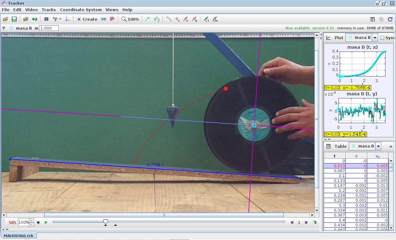
Figure 2: Experimental setup as seen inside the Tracker graphical user interface. The ramp is used as the reference length (blue segment). The $x$ axis is parallel to the ramp (in magenta). It can be noted that the path followed by the disk center (in cyan) has the same direction as the $x$ axis. The attached particle’s path (in red) is a cycloid, as expected from the rolling without slipping condition. The plumb line gives a fixed reference direction for measuring angles.

IV Results

Fig. 3 summarizes the information we extracted from videos to validate our model and answer the initial motivating questions. Panel $(a)$ of this figure shows the measured $x$ coordinate as a function of time $t$ for various typical cases. From this data, we calculated the speed of the disk center by means of numerical differentiation using the midpoint rule NoteDeriv (16) $\dot{x}(t_{i})=\frac{1}{2\Delta t}\left(x(t_{i}+\Delta t)-x(t_{i}-\Delta t)\right)$. The resulting values are displayed in panel $(b)$ within the same figure. With these values of ($x$,$\dot{x}$), we checked the assumption of mechanical energy conservation upon which the model rests, by calculating the kinetic and potential energy at each frame. It is worth pointing out that normally this is an issue not addressed experimentally within the subject of 2D rigid body motions in basic mechanics courses, and is only treated theoretically from the viewpoint of Coulomb’s classic friction model. With this purpose, in panel $(c)$ we exhibit the temporal evolution of mechanical energy for the previous cases. When comparing initial and final absolute values we can see a slight decrease of mechanical energy. For a better appreciation, this change is assessed by calculating the relative variation $\Delta e(t_{i})=\left(E(t_{i})-E(0)\right)/E(0)$, whose evolution is shown in panel $(d)$. These variations are on average of about 5% or less, as reported by Carnevali for low speeds, Carnevali-May-AJP-2005 (6) and only exceptionally reach 10%. The reason for the extreme values of the relative variation is the following: at high speeds the image of the disk center becomes “fuzzy” due to the finite time of image capture between frames, increasing the uncertainty in position and speed, and consequently in energy. This explains the wild oscillations and the local deviation from the average behavior near maxima of $\dot{x}$ which can be seen in $(d)$. In view of these results we conclude that the hypothesis of conservation of mechanical energy (3) holds reasonably well for our purposes.

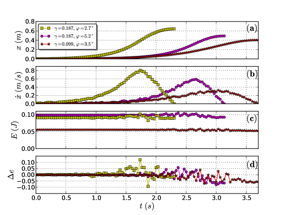
Figure 3: Position, velocity and energy evolution for various representative cases. Panel $(a)$ shows the $x$ coordinate of the disk center as a function of time. Panel $(b)$ is the velocity of the disk center as calculated from data in $(a)$ by numerical differentiation. Panel $(c)$ displays the mechanical energy for the same data, and $(d)$ exhibits the time evolution of the relative energy variation with respect to the initial mechanical energy.

To verify the prediction (9), we experimentally determined the minimum initial angle from the vertical $\theta_{\mathrm{min}}^{e}$ at which the disk begins to move upwards, for various values of the inclination angle $\varphi$. In Fig. 4, the pairs $\left[\sin(\varphi),\sin(\theta_{\mathrm{min}}^{e})\right]$ are plotted for $\gamma=0.187$ (blue circles) and compared with the theoretical prediction (solid red line). The linear fit (discontinuous blue line) yields $\gamma=0.196$, which falls within the experimental uncertainty range $\Delta\gamma=0.01$ around the value calculated using (4), and a discrepancy in the y-intercept compatible with the estimated uncertainties for the angles $(\Delta\varphi=0.4,\ \Delta\theta_{\mathrm{min}}^{e}=1.5^{\circ})$. Consequently, we can state that the prediction is confirmed within the error margins of the measurement, and that the answer for question 1 is given by equation (9). Notice that the measured angle $\theta_{\mathrm{min}}^{e}$ is always bigger than the theoretical one for a given $\varphi$. This is a consequence of the manual method used to initiate the motion in the desired (ascending) sense, considering that the minimum angle corresponds to an unstable equilibrium.

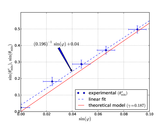
Figure 4: Sine of the theoretical ($\theta_{\mathrm{min}}$) and experimental ($\theta_{\mathrm{min}}^{e}$) values of the minimum initial angle as a function of the sine of plane inclination $\varphi$ for the observed value of $\gamma=0.187$. The solid (red) line is the theoretical model prediction for this value of $\gamma$, given by equation (9). (Blue) circles indicate measured data. The discontinuous (blue) line represents the linear fit of the experimental values, whose equation is shown.

Finally, to corroborate (16) we plot in Fig. 5 the measured pairs $(x,\dot{x})$ for several values of the inclination angle $\varphi$ and two values of the eccentricity parameter $(\gamma=0.094,\ \gamma=0.187)$. Lines represent the model prediction (16) for the measured values of $\gamma,\ \theta_{0}$ and $\varphi$. The color bands centered at these lines indicate the theoretical prediction uncertainty arising from uncertainties in the measurement of parameters. In all the cases investigated, the model explains well the experimental values, as can be observed in both figures. We conclude that equation (16) answers question 2 in phase space.

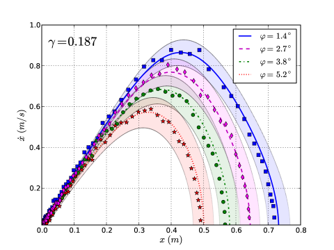
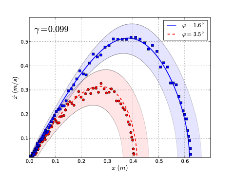
Figure 5: Motion of the system in phase space for different values of $\varphi$ and $\gamma$. Symbols represent the experimental values obtained from video. Lines indicate the theoretical model prediction –given by equation (16)– for the corresponding values of $\varphi$ and $\gamma$. Bands around these lines show the theoretical model uncertainty arising from uncertainties in the model parameters.

V Conclusions

In this paper, we presented a modification of a textbook problem in rigid body dynamics which can be used to integrate theoretical and experimental issues in a first university mechanics course. The proposal may be implemented as a short laboratory project, motivated by an easily reproducible demonstration of the phenomenon and the simple questions posed in the introduction. Besides, we obtained very satisfactory original results resorting only to readily available tools and methods. We confirmed the model predictions with an accuracy compatible with the quality of the experimental observations, complementing previous results reported in the literature for similar systems. The same methodology can be applied to other variants of traditional problems in mechanics, being a valuable resource in elementary physics teaching.

References

- (1) D. Halliday, R. Resnick, and J. Walker, Fundamentals of Physics - Extended, 10th. edition (John Wiley & Sons, 2013), chapter 11.
- (2) Arthur Good (a.k.a. Tom Tit), La science amusante (3e. s rie) - 100 nouvelles experiences, 29e ed. (Larousse, 1906). The article in question appears on page 9. A digital version (in French) can be downloaded from the Biblioth que nationale de France at <http://gallica.bnf.fr/ark:/12148/bpt6k930558v/f8.image.r=tom%20tit.langEN>.
- (3) W.F.D. Theron, “The rolling motion of an eccentrically loaded wheel,” Am. J. Phys. 68, 812–820 (2000).
- (4) W.F.D. Theron and M.F. Maritz, “The amazing variety of motions of a loaded hoop,” Math. Comp. Model. 47, 1077–1088 (2008).
- (5) M.F. Maritz and W.F.D. Theron, “Experimental verification of the motion of a loaded hoop,” Am. J. Phys. 80, 594–598 (2012).
- (6) A. Carnevali and R. May, “Rolling motion of non-axisymmetric cylinders,” Am. J. Phys. 73, 909–913 (2005).
- (7) A. Taylor and M. Fehrs, “The dynamics of an eccentrically loaded hoop,” Am. J. Phys. 78, 496–498 (2010).
- (8) R.W. Gomez, J.J. Hernandez-Gomez, and V. Marquina, “A jumping cylinder on an inclined plane,” Eur. J. Phys. 33, 1359–1365 (2012).
- (9) S. Gil, H.D. Reisin, and E.E. Rodríguez, “Using a digital camera as a measuring device,” Am. J. Phys. 74, 768 (2006).
- (10) D. Brown and A. J. Cox,“Innovative Uses of Video Analysis,” Phys. Teach. 47, 145 (2009).
- (11) Tracker is an open source software for video analysis, focused in physics teaching. It is written in Java, so it can be run on multiple computer platforms (GNU/Linux and Windows, among others). The program and its documentation can be found at <http://www.cabrillo.edu/~dbrown/tracker/>. Tracker is part of the Open Source Physics project <http://www.opensourcephysics.org/>, which promotes the use of computational resources in physics teaching.
- (12) Python is a high-level, interpreted programming language, suitable both for learning programming and for advanced scientific computing. Extensive documentation can be found in <http://www.python.org>. Currently, there is an increasing trend in the use of Python among the scientific community due to the availability of numerous libraries for scientific and engineering applications, such as SciPy <http://www.scipy.org/> and matplotlib <http://matplotlib.sourceforge.net/>.
- (13) is a constant inertia parameter, dependent on the specific mass distribution with cylindrical symmetry.
- (14) For the same purpose could be used any camera, phone or tablet properly aligned and with fixed focus, as auto-focus can lead to undesirable changes between frames.
- (15) Supplemental material at <https://drive.google.com/folderview?id=0B1_k1yO4m0kDNE1uX0R4LXpWQWs&usp=sharing>.
- (16) Numerical differentiation is an operation that should be applied with care, as it tends to amplify the noise present in the input data. To minimize this effect, we’ve put special care in determining the values . We could have used a method of higher order Theron-Maritz-MathCompModel-2008 (4) but opted for the midpoint rule for three reasons: it is the method used by Tracker to calculate speeds, thus avoiding further processing of the data; higher order formulas provided virtually identical results; the midpoint formula is easier to justify heuristically in the context of a first course in mechanics, as details related to data analysis and numerical calculation generally exceeds the preparation of students at this level. For more details, see next reference. Burden-Faires (17)
- (17) R.L. Burden, J.D. Faires: Numerical Analysis, 9th. ed. (Cengage Learning, 2010).