Hybrid spin and valley quantum computing with singlet-triplet qubits

Abstract

The valley degree of freedom in the electronic band structure of silicon, graphene, and other materials is often considered to be an obstacle for quantum computing (QC) based on electron spins in quantum dots. Here we show that control over the valley state opens new possibilities for quantum information processing. Combining qubits encoded in the singlet-triplet subspace of spin and valley states allows for universal QC using a universal two-qubit gate directly provided by the exchange interaction. We show how spin and valley qubits can be separated in order to allow for single-qubit rotations.

Introduction.—An alternative to single-spin qubits in quantum dots LoDi1998 is to encode each qubit in a double quantum dot (DQD) within the two-dimensional subspace spanned by the spin singlet $\left|S\right>=(\left|01\right>-\left|10\right>)/\sqrt{2}$ and the triplet $\left|T_{0}\right>=(\left|01\right>+\left|10\right>)/\sqrt{2}$ kloeffel_loss_review_2013 , with $\left|0\right>=\left|\uparrow\right>$, $\left|1\right>=\left|\downarrow\right>$. For this singlet-triplet qubit, single-qubit rotations can be realized by the exchange interaction Petta et al. (2005); Foletti et al. (2009) and a gradient in the magnetic field Foletti et al. (2009); two-qubit gates have been proposed based on exchange interaction Levy (2002); Benjamin (2001); Klinovaja et al. (2012); PhysRevB.86.205306 or electrostatic coupling Taylor_natphys ; Stepanenko2007 ; PhysRevB.84.155329 . An electrostatically controlled entangling gate has been realized experimentally PhysRevLett.107.030506 ; Shulman . Quantum computing (QC) with single-spin and/or single-valley qubits requires rotations of single-valley and/or single-spin degrees of freedom (DOFs) rohling_burkard . In this Letter, we show that, by extending the concept of $S$-$T_{0}$ qubits to electrons with spin and valley DOFs, the exchange interaction together with Zeeman gradients directly provides universal QC. Single-qubit rotations are feasible when the spin and the valley $S$-$T_{0}$ qubits are stored in separated DQDs, whereas in a dual-used DQD, i.e., containing the $S$-$T_{0}$ spin and valley qubits, a two-qubit gate is obtained by exchange interaction rohling_burkard . Here, we focus on operations separating and bringing together spin and valley qubits, allowing for a universal set of single- and two-qubit operations in a quantum register.

The valley DOF describes the existence of nonequivalent minima (maxima) in the conduction (valence) band in several materials such as silicon zwanenburg , graphene castro_neto , carbon nanotubes kuemmeth , aluminum arsenide shayegan , or transition metal dichalcogenide monolayers xiao ; kormanyos . A twofold valley degeneracy can be considered as a qubit. In particular, silicon-based heterostructures have aroused much interest as hosts for electron spin qubits zwanenburg due to long relaxation feher_gere and coherence tyryshkin times. Valley states in silicon structures have been under intense theoretical boykin:115 ; nestoklon ; chutia ; PhysRevB.80.081305 ; PhysRevB.82.155312 ; PhysRevB.82.245314 ; PhysRevB.84.155320 ; baena ; drumm ; de_michelis ; gamble2012 ; gamble2013 ; tahan_joynt_2013 ; jiang ; genetic_design ; dusko and experimental xiao:032103 ; borselli:123118 ; borselli:063109 ; lim ; simmons ; PhysRevB.86.115319 ; yang2013 ; PhysRevLett.111.046801 ; kott ; roche ; yuan ; yamahata ; hao ; goswami investigation recently. The valley degeneracy is often considered problematic for spin QC eriksson ; trauzettel , and valley splitting is used to achieve pure spin exchange interaction maune . Also, theories for the manipulation of valley qubits have been developed for carbon nanotubes PhysRevLett.106.086801 , graphene PhysRevB.84.195463 ; PhysRevB.88.125422 , and silicon PhysRevB.82.205315 ; PhysRevLett.108.126804 ; PhysRevB.86.035321 . While these approaches consider valley and spin qubits separately, we investigate a hybrid quantum register containing both spin and valley qubits.

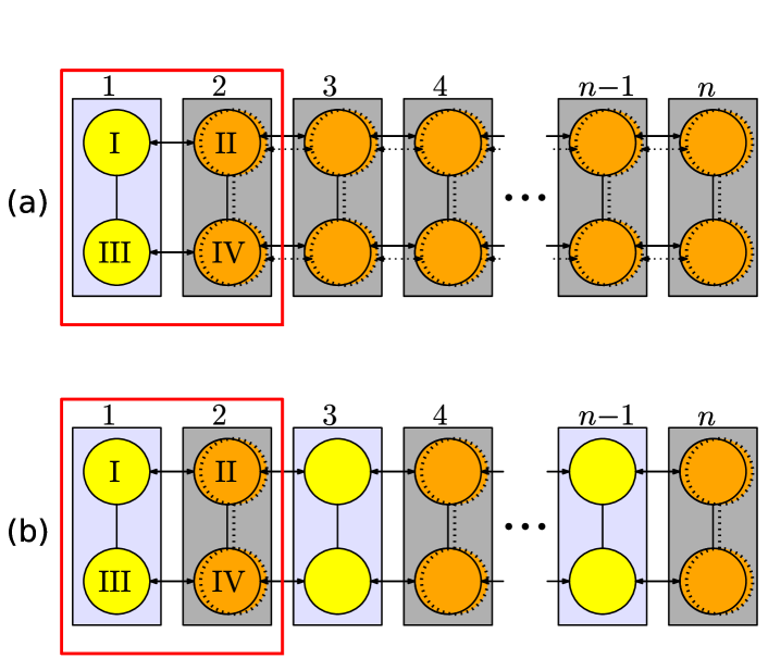
Figure 1: Two quantum registers for QC with spin and valley singlet-triplet qubits. The single (yellow) circles denote dots with spin DOF only (valley degeneracy lifted) hosting auxiliary spins, whereas the double (orange) circles denote dots with both spin and valley DOFs storing one spin and one valley $S$-$T_{0}$ qubit. The lines within the DQDs represent the exchange interaction (a single line for spin-only dots, solid and dotted lines for spin and valley), which can realize single-qubit gates when the spin qubit is transferred to the spin-only DQD and a two-qubit gate when spin and valley qubits are in the same DQD. The arrows between dots from neighboring DQDs represent ${\rm SWAP}$ operations, interchanging the spin (solid arrow) or valley (dotted arrow) state between these dots. Register (b) has more auxiliary dots; quantum gate sequences are shorter than in (a).

Two different types of hybrid spin-valley singlet-triplet quantum registers will be studied (Fig. 1). Both setups comprise two kinds of DQDs: one (e.g.,dots I and III) with a spin DOF only (simple yellow circles), where the valley degeneracy does not exist or has been lifted and another kind of DQD (e.g., II and IV) with both spin and twofold valley DOF (double orange circles). The elementary building block of the proposed quantum register consists of two DQDs, one of each kind (red rectangle in Fig. 1). We use the singlet $\left|S\right>$ and triplet $\left|T_{0}\right>$ states of spin and valley in DQD 2 as the logical qubits. The spins in DQD 1 are spin polarized, $\left|\uparrow\uparrow\right>$ or $\left|\downarrow\downarrow\right>$, which is needed for the single-qubit gates. The exchange interaction between dots II and IV, described in general by a Kugel-Khomskii Hamiltonian kugel_khomskii_1973 ; rohling_burkard , already leads to a universal two-qubit gate between the spin and the valley singlet-triplet qubits in the same DQD rohling_burkard . Single-qubit gates for the logical qubits can be achieved by applying two spin-only SWAP gates, between I and II and between III and IV, interchanging the spin $S$-$T_{0}$ qubit in DQD 2 with the polarized ancilla spins in DQD 1, without affecting the valley state. The single-qubit gates of the spin and the valley qubits can be realized by exchange interaction and a spin or valley Zeeman gradient Foletti et al. (2009); PhysRevLett.108.126804 . State preparation and measurements can be done for spatially separated spin and valley qubits. Changing the detuning within the DQD maps exactly one state of the qubit to a state with both electrons in one dot due to the Pauli exclusion principle kane_nature ; vandersypen . The charge state can be detected by a quantum point contact Petta et al. (2005). State preparation works in the opposite direction, starting from a ground state with both electrons in one dot at large detuning. Before explaining how to perform arbitrary quantum gates in the registers, we propose a realization of an elementary gate in our scheme, the spin-only SWAP gate.

Model.—We consider the system consisting of dots I and II in Fig. 1, i.e., one dot with a spin DOF only and the other dot with spin and twofold valley DOF. We model the physics in this DQD by the Hamiltonian $H=H_{0}+H_{T}+H_{V}$. The influence of the detuning $\varepsilon$ and the Coulomb repulsion energy between two electrons on the same site, $U$, is given by $H_{0}=\varepsilon(\hat{n}_{1}-\hat{n}_{2})/2+U\sum_{i=1,2}\hat{n}_{i}(\hat{n}_{i}-1)/2$ with the number operators $\hat{n}_{1}=\sum_{s}\hat{c}_{1s}^{\dagger}\hat{c}_{1s}$ and $\hat{n}_{2}=\sum_{s,v}\hat{c}_{2sv}^{\dagger}\hat{c}_{2sv}$ where $\hat{c}_{1s}^{(\dagger)}$ annihilates (creates) an electron with spin $s=\uparrow,\downarrow$ in dot I and $\hat{c}_{2sv}^{(\dagger)}$ annihilates (creates) an electron with spin $s=\uparrow,\downarrow$ and valley $v=\pm$ in dot II. Electron hopping is described by $H_{T}=\sum_{s,v}t_{v}\hat{c}_{1s}^{\dagger}\hat{c}_{2sv}+h.c.$ and the valley splitting by $H_{V}=h\sum_{s}(\hat{c}_{2s+}^{\dagger}\hat{c}_{2s+}-\hat{c}_{2s-}^{\dagger}\hat{c}_{2s-})\equiv h\sigma_{z}$, where $\sigma_{z}$ is a Pauli matrix acting on the valley space. The sums run over $s=\uparrow,\downarrow$ and $v=\pm$. The valley-dependent hopping elements $t_{\pm}$ can be expressed by PhysRevB.82.205315 $t_{\pm}=t(1\pm e^{i\varphi})/2$ with real parameters $t$ and $\varphi$, and $h$ can be tuned in silicon by the electrically controlled confinement potential yang2013 and in graphene by an out-of-plane magnetic field PhysRevB.79.085407 . For two electrons in dots I and II, there are 15 possible states, one with (2,0), six with (0,2), and eight with (1,1) charge distribution between dots I and II. In the limit $t\ll|h+(U\pm\varepsilon)|,|h-(U\pm\varepsilon)|$, a Schrieffer-Wolff transformation burkard_imamoglu yields the effective Hamiltonian Supplemental

$$H_{\rm eff} = \left[(A\cos\varphi{+}B)\mathds{1}+(A{+}B\cos\varphi)\sigma_{z}+B\sin\varphi\,\sigma_{y}\right]P_{S}$$ (1)

$$+\tilde{h}\sigma_{z}+C\left[(1-\cos\varphi)\mathds{1}-\sin\varphi\,\sigma_{y}\right].$$

Here, $P_{S}$ is the projector on the spin singlet $\left|S\right>=(\left|\uparrow\downarrow\right>-\left|\downarrow\uparrow\right>)/\sqrt{2}$, $A=4t^{2}Uh\varepsilon/[(h-U-\varepsilon)(h+U-\varepsilon)(h-U+\varepsilon)(h+U+\varepsilon)]$, $B=A(h^{2}{+}\varepsilon^{2}{-}U^{2})/2h\varepsilon$, $\tilde{h}=h\{1+t^{2}(1{-}\cos\varphi)/[2(h{-}U{+}\varepsilon)(h{+}U{-}\varepsilon)]\}$, and $C=t^{2}(U{-}\varepsilon)/[2(h{-}U{+}\varepsilon)(h{+}U{-}\varepsilon)]$. Note that $H$ and $H_{\rm eff}$ are block diagonal in the spin singlet-triplet basis, similar to the situation in Ref. PhysRevB.82.205315 . We aim at using the term proportional to $P_{S}$ to perform a spin-only ${\rm SWAP}$ gate, interchanging the spin information of dots I and II independently of the valley state. We will show that this is possible despite the valley dependence of $H_{\rm eff}$.

Spin-only SWAP gate.—For the valley-degenerate case $h=0$, Eq. (1) simplifies to the exchange Hamiltonian

$$H^{0}_{\rm eff}=-JP_{S}P_{k}-\tilde{J}P_{k^{\perp}},$$ (2)

where $J=4t^{2}U/(U^{2}-\varepsilon^{2})$ and $\tilde{J}=t^{2}/(U-\varepsilon)$. The first term is proportional to $P_{S}$ and to the projector $P_{k}$ on the valley state $\left|k\right>=[(1+e^{-i\varphi})\left|+\right>+(1-e^{-i\varphi})\left|-\right>]/2$ occupied by an electron after hopping from dot I to dot II. The second term is spin independent and $\propto P_{k^{\perp}}=\left|k^{\perp}\right>\left<k^{\perp}\right|$, where $\left|k^{\perp}\right>=[(1-e^{-i\varphi})\left|+\right>+(1+e^{-i\varphi})\left|-\right>]/2$ is orthogonal to $\left|k\right>$. Both contributions originate from the Pauli principle: virtual hopping between dots I and II is possible only if the participating (0,2) or (2,0) state is antisymmetric. Virtual hopping from (1,1) to (0,2) and back is $\propto t^{2}/(U-\varepsilon)$ and dominates for $\varepsilon\approx U$; if the valley state in the right dot is $\left|k^{\perp}\right>$, this channel is open, independently of the spin states, as the valley state $\left|k\right>$ used within the virtual hopping is empty. If the valley state is $\left|k\right>$, the spins have to be in a singlet to allow for an antisymmetric (0,2) state. Virtual hopping from (1,1) to (2,0) and back requires a valley state $\left|k\right>$ in the right dot, as $\left|k^{\perp}\right>$ has no overlap with the state in the left dot; it further requires the spins to be a singlet to obey Fermi-Dirac statistics.

For $|U+\varepsilon|\ll U$, $\tilde{J}$ can be neglected and the time evolution $U_{0}(\phi)=\exp[-i\int_{0}^{\tau}d\tau^{\prime}H^{0}_{\rm eff}(\tau^{\prime})/\hbar]$ with $\phi=\int_{0}^{\tau}d\tau^{\prime}J(\tau^{\prime})/\hbar$ can be computed easily: $U_{0}(\phi)=\mathds{1}+(e^{i\phi}-1)P_{S}P_{k}$. If the conditions $\tilde{J}\approx 0$, $\varphi=\pi/2$, and controllability of the valley splitting $h$ are fulfilled, we obtain a spin-only SWAP gate with the sequence ${\rm SWAP}\equiv\mathds{1}-2P_{S}=\sigma_{z}U_{0}(\pi)\sigma_{z}U_{0}(\pi)$. Here, $h$ is turned off or at least made negligibly small during the exchange interaction but dominates over exchange in between to realize the valley gate $\sigma_{z}$.

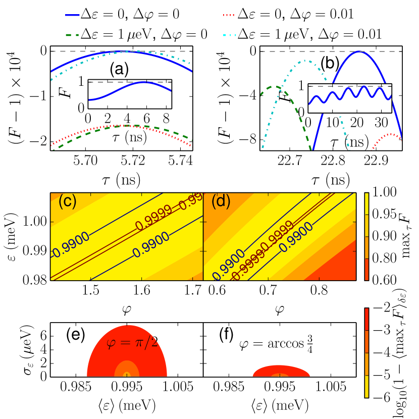
Figure 2: Fidelity $F$ of the time evolution operator $U_{\rm eff}(\tau)$ describing the exchange interaction between a spin-only dot and a spin-valley dot with respect to thes spin SWAP gate according to Eq. (3). The parameters are chosen to be $U=1$ meV, $h=0.1$ meV, and $t=6~{}\mu$eV. (a),b) $F$ maximized over the gate time $\tau$ (scale bar). The detuning is chosen to be $\varepsilon=\sqrt{U^{2}-h^{2}}+\Delta\varepsilon\approx 0.995~{}{\rm meV}+\Delta\varepsilon$ and the phase in the hopping matrix elements, $\varphi=\frac{\pi}{2}+\Delta\varphi$ (a) and $\varphi=\arccos\frac{3}{4}+\Delta\varphi$ (b). (c),d) Contour plots of maximal fidelity in dependence of $\varepsilon$ and $\varphi$. The maximum over $\tau$ is taken numerically by searching around the first (c) and fourth (d) local maximum. At $\Delta\varphi=0$, $\Delta\varepsilon=0$, $F=1$ can be realized. A shift in valley hopping phase, $\Delta\varphi$, can be compensated by adjusting $\varepsilon$. (e),f) Averaged fidelity for a Gaussian distribution of $\varepsilon$ with variance $\sigma_{\varepsilon}^{2}=\langle\varepsilon^{2}\rangle-\langle\varepsilon\rangle^{2}$. The maximization over time is done for the value $\varepsilon=\langle\varepsilon\rangle$ at the first (e) and fourth (f) local maximum.

If $\tilde{h}\sigma_{z}$ is the dominant contribution in $H_{\rm eff}$, we find parameters which allow for a spin SWAP gate (Figs. 2 and 3). We denote the time evolution according to a time-independent $H_{\rm eff}$ at time $\tau$ with $U_{\rm eff}(\tau)$ and consider the average gate fidelity Pedersen200747

$$F=\max_{\alpha}\frac{8+|\operatorname{Tr}[e^{i\alpha\sigma_{z}}U_{\rm eff}(\tau){\rm SWAP}^{\dagger}]|^{2}}{72}$$ (3)

where we maximize over a $z$ rotation in valley space, which is unimportant for the logical valley qubit in the singlet-triplet subspace. For the spin SWAP gate applied between dots I and II and between dots III and IV, the valley $z$ rotation can be different. This difference is equivalent to a rotation of the $S$-$T_{0}$ valley qubit, which can be corrected afterwards. In the case $|A|,|B|,|C|\ll|\tilde{h}|$ considered here, we determine the phase $\alpha$ for the maximum in Eq. (3) analytically Supplemental . Figure 2 shows $F$ for a detuning around $\varepsilon=\sqrt{U^{2}{-}h^{2}}$, where the parameter $B=0$. If furthermore $C$ is negligible, we obtain $U_{\rm eff}(\tau_{n})={\rm SWAP}$ for $\varphi=\arccos\frac{n}{n+1}$ and $\tau_{n}=(n+1)\pi\hbar/A$. In Fig. 2, the situation is shown for $n=0$ and $n=3$. Figure 3 reveals that, also for other parameter regimes, $U_{\rm eff}(\tau)$ can be the spin SWAP gate with a high fidelity. The time $\tau$ where the maximal fidelity is reached is determined numerically. We include quasistatic charge noise, which was found to be important for GaAs DQDs PhysRevLett110.146804 , by averaging $F$ over a Gaussian distribution of $\varepsilon$. We find that for the fluctuating bias $\varepsilon$ with standard deviation $\sigma_{\varepsilon}=\sqrt{\langle\varepsilon^{2}\rangle-\langle\varepsilon\rangle^{2}}\approx\mu$eV the fidelity can be as high as $F\gtrsim 0.9999$ [see Figs. 2(e), 2(f), Fig. 3(e), and 3(f)]. We expect the noise sensitivity of $U_{\rm eff}(\tau)$ to be similar to exchange gates with spin DOF only Supplemental . Spin singlet-triplet qubits in silicon also suffer from coupling to nuclear spins, but recent work concludes that charge noise is the dominating source of dephasing APL102_232108 .

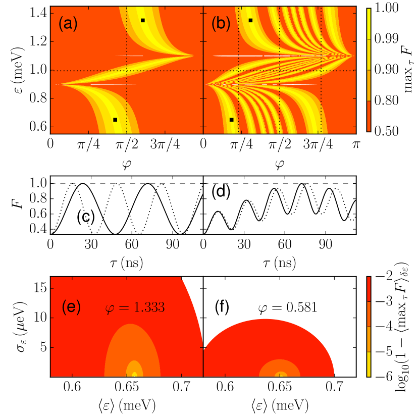
Figure 3: Fidelity $F$ for a broad range of the detuning $\varepsilon$ and the phase $\varphi$ in the hopping matrix elements, using the same parameters $U$, $h$, and $t$ as in Fig. 2. (a),b) $F$ maximized over the gate time $\tau$. We consider the first (a) and fourth (b) local maximum of $F$ as a function of $\tau$. The black squares indicate the positions in parameter space for the time-dependent plots (c,d), namely, $\varepsilon=1.35\,{\rm meV}$ for the solid lines and $\varepsilon=0.65\,{\rm meV}$ for the dotted lines in (c),d), $\varphi=1.9$ (solid line), $\varphi=1.333$ (dotted line) in (c), and $\varphi=0.972$ (solid line), $\varphi=0.581$ (dotted line) in (d). The horizontal dotted lines in (a),b) represent $\varepsilon=\sqrt{U^{2}{-}h^{2}}$, and the vertical dotted lines belong to values of $\varphi$ being $\frac{\pi}{2}$ (a),b) and $\arccos\frac{3}{4}$, $\pi-\arccos\frac{3}{4}$ (b). Note that the Schrieffer-Wolff transformation breaks down close to $\varepsilon=U\pm h$. (e),f) Averaged fidelity for a Gaussian distribution of $\varepsilon$ with $\sigma_{\varepsilon}^{2}=\langle\varepsilon^{2}\rangle-\langle\varepsilon\rangle^{2}$. The maximum in time is determined for $\varepsilon=\langle\varepsilon\rangle$ at the first (e) and fourth (f) local maximum. The fidelity, $F$ is more robust at the first local maximum.

Hybrid quantum register.—Now we consider the entire register of $n$ DQDs built in two different ways (Fig. 1) and prove that universal QC is possible in these two registers. It is sufficient to show that single-qubit gates for every qubit and a universal two-qubit gate between arbitrary qubits can be performed divincenzo1995 .

In the register Fig. 1 (a), there is only one spin-only DQD, at position 1, and $(n-1)$ DQDs with spin and valley DOFs. Single-qubit gates for the qubits in the $k$th DQD, $1<k\leq n$ can be performed by first transferring these qubits, both spin and valley, to DQD 2. This is done by applying ${\rm SWAP}_{\rm spin}\otimes{\rm SWAP}_{\rm valley}$ gates in the upper and the lower row of the register which allows interchanging the information of DQD $k$ with $k-1$ and so on. The ${\rm SWAP}_{\rm spin}\otimes{\rm SWAP}_{\rm valley}$ gate is provided directly from the exchange interaction rohling_burkard . Second, the spin-only ${\rm SWAP}$ gate transfers the spin qubit into DQD 1, and in return the polarized ancilla spins into DQD 2. Now single-qubit operations can be performed for the spin $S$-$T_{0}$ qubit in DQD 1 and for the valley in DQD 2. The universal two-qubit gate between qubits in DQD $k$ and in DQD $m$ require transferring the qubits from these dots to DQDs 2 and 3. Then applying the spin-only ${\rm SWAP}$ moves the spin qubit from DQD 2 to DQD 1. The ${\rm SWAP}_{\rm spin}\otimes{\rm SWAP}_{\rm valley}$ gate between DQDs 2 and 3 and another spin-only ${\rm SWAP}$ yield a situation where the spin qubit from DQD $k$ and the valley qubit from DQD $m$ are together in DQD 2, where the universal two-qubit gate can be applied rohling_burkard . If two valley qubits or two spin qubits need to be involved in the two-qubit gate, the spin and the valley qubits can be interchanged when they are in DQD 2. The average number of additional ${\rm SWAP}$ gates needed for transferring qubits to the DQD at one end of the register before the desired gates can be applied is on the order of $n^{2}$ Supplemental . The register Fig. 1 (b) contains a spin-only DQD for every spin-valley DQD. This allows for single-qubit operations without transferring qubits through the whole register. Two-qubit gates between arbitrary qubits can be performed as spins can be moved within the entire register by spin-only ${\rm SWAP}$ gates. It is crucial to achieve high-fidelity spin-only and spin-valley SWAP gates. Errors in those operations can lead to leakage as spin and valley could leave the singlet-triplet subspaces.

Materials.—We now focus on the materials which may provide the necessary properties for realizing our QC scheme. A natural choice seems to be a hybrid structure of one material without and one with a valley degeneracy where the hopping parameters $t$ and $\varphi$ across the interface can be controlled.

The sixfold valley degeneracy of bulk silicon is typically split off by a (001) interface RevModPhys.54.437 ; PhysRevB.61.2961 ; herring ; PhysRev.101.944 ; PhysRevB.34.5621 ; people_bean ; PhysRevB.48.14276 ; schaeffler ; the two lower valleys of interest, denoted $\left|z\right>$ and $\left|\overline{z}\right>$, are coupled by valley-orbit interaction, described by the complex matrix element $V_{\rm VO}$ PhysRevB.80.081305 . In experiment, a valley splitting $2|V_{\rm VO}|$ in lateral silicon quantum dots of 0.1-1 meV has been reported xiao:032103 ; borselli:123118 ; borselli:063109 ; lim ; simmons ; PhysRevB.86.115319 ; yang2013 ; PhysRevLett.111.046801 . Electrical tunability in the range from 0.3 to 0.8 meV was demonstrated yang2013 . Calculations show that while $\arg(V_{\rm VO})$ is only slightly influenced by an applied electric field PhysRevB.86.035321 , it depends on the conduction band offset PhysRevB.84.155320 ; thus, a structure with an alternating top layer material, e.g., SiO₂ and SiGe or Si_1-xGe_x with a varying $x$ could provide the difference in $\arg(V_{\rm VO})$, i.e. $\varphi\neq 0$, which is needed in our scheme between dots I and II and between III and IV, while $\arg(V_{\rm VO})$ should be the same in dot II and IV. Whereas the band offset difference is higher between Si/SiO₂ and Si/SiGe, charge traps at the Si/SiO₂ interface can be a source for noise APL95_0723102 ; nevertheless, spin blockade was demonstrated in Si/SiO₂ structures with a reduced density of traps SciRep1_110 . Furthermore, one requires a large valley splitting in dots I and III, which results in a situation where effectively only one valley state participates in the dynamics.

Graphene provides a twofold valley degeneracy and should allow for a two-dimensional array of quantum dots. Theory shows that the valley state is affected by a magnetic field perpendicular to the graphene plane PhysRevB.79.085407 and in graphene nanoribbons also by the boundary conditions trauzettel .

Dual hybrid register.—Interchanging the roles of spin and valley yields DQDs with spin and valley DOF and with valley DOF only. A strong local magnetic field could yield conditions where only the lowest spin states in this DQD have to be taken into account; the spin Zeeman splitting has to be large compared to the exchange interaction, e.g., 0.01 meV in Ref. Petta et al. (2005). To achieve a different phase between these spin states and the spins of the energy eigenstates in the spin-valley dots, the direction of the magnetic field has to be different for different dots. Therefore, this alternative approach seems to have less stringent requirements from the material point of view (phase of valley states can be the same), but would require a field gradient of several Tesla on a nanometer scale.

Conclusion.—In conclusion, we have shown that combining spin and valley singlet-triplet qubits allows for a new hybrid spin-valley QC scheme. Necessary conditions are control over the Zeeman splitting for spin and valley as well as over the phase of the valley states, the realization of high-fidelity ${\rm SWAP}$ operations, and long enough valley coherence times. The concept relies crucially on the controlled coexistence of spin and valley qubits allowing for universal QC based on the electrically tunable exchange interaction.

Acknowledgements.—We thank the DFG for financial support under Programs No. SPP 1285 and No. SFB 767.

Supplemental Material

I A. Schrieffer-Wolff transformation

The Schrieffer-Wolff transformation for our Hamiltonian from the main text,

$$\tilde{H}=e^{-S}He^{S}\approx H_{0}+H_{V}+\frac{[H_{T},S]}{2}=\left(\begin{array}[]{cc}H_{\rm eff}&0\\ 0&H_{\rm as}\end{array}\right),$$ (A1)

is done similar to the situation without the valley degree of freedom [S1]. The block $H_{\rm eff}$ describes the physics in the low-energy subspace, which has approximately (1,1) charge configuration when the detuning $\varepsilon$ is close to zero. We can perform the transformation for the spin singlet subspace and for the spin triplet subspaces separately. The projection on the three-dimensional subspace including one spin triplet, is spanned e.g. by the basis $\{\left|\uparrow,{\uparrow\!+}\right>=\hat{c}_{1\uparrow}^{\dagger}\hat{c}_{2\uparrow+}^{\dagger}\left|0\right>,\left|\uparrow,{\uparrow\!-}\right>\hat{c}_{1\uparrow}^{\dagger}\hat{c}_{2\uparrow-}^{\dagger}\left|0\right>,\left|0,{\uparrow\!+}{\uparrow\!-}\right>=\hat{c}_{2\uparrow+}\hat{c}_{2\uparrow-}\left|0\right>\}$ for the $T_{+}$ triplet and described by the Hamiltonian,

$$H_{\rm Triplet}=\left(\begin{array}[]{ccc}h&0&-t_{-}\\ 0&-h&t_{+}\\ -t_{-}^{*}&t_{+}^{*}&U-\varepsilon\end{array}\right).$$ (A2)

For the spin singlet subspace we have in the basis $\{(\left|\uparrow,\downarrow\!+\right>-\left|\downarrow,\uparrow\!+\right>)/\sqrt{2},(\left|\uparrow,\downarrow\!-\right>-\left|\downarrow,\uparrow\!-\right>)/\sqrt{2},(\left|0,{\uparrow\!+}{\downarrow\!-}\right>+\left|0,{\uparrow\!-}{\downarrow\!+}\right>)/\sqrt{2},\left|\uparrow\downarrow,0\right>,\left|0,{\uparrow\!+}{\downarrow\!+}\right>,\left|0,{\uparrow\!-}{\downarrow\!-}\right>\}$, the Hamiltonian

$$H_{\rm Singlet}=\left(\begin{array}[]{cccccc}h&0&t_{-}&\sqrt{2}t_{+}^{*}&\sqrt{2}t_{+}&0\\ 0&h&t_{+}&\sqrt{2}t_{-}^{*}&0&\sqrt{2}t_{-}^{*}\\ t_{-}^{*}&t_{+}^{*}&U-\varepsilon&0&0&0\\ \sqrt{2}t_{+}&\sqrt{2}t_{-}&0&U+\varepsilon&0&0\\ \sqrt{2}t_{+}^{*}&0&0&0&U-\varepsilon+2h&0\\ 0&\sqrt{2}t_{-}^{*}&0&0&0&U-\varepsilon-2h\end{array}\right).$$ (A3)

The anti-Hermitian matrix $S$ should obey $[H_{0}+H_{V},S]=-H_{T}$, which is fulfilled if the blocks corresponding to the singlet and triplet subspaces are given by

$$S_{\rm Triplet}=\left(\begin{array}[]{ccc}0&0&\frac{t_{-}}{h-U+\varepsilon}\\ 0&0&\frac{-t_{+}}{-h-U+\varepsilon}\\ \frac{-t_{-}^{*}}{h-U+\varepsilon}&\frac{t_{+}^{*}}{-h-U+\varepsilon}&0\end{array}\right)$$ (A4)

and

$$S_{\rm Singlet}=\left(\begin{array}[]{cccccc}0&0&\frac{-t_{-}}{h-U+\varepsilon}&\frac{\sqrt{2}t_{+}^{*}}{-h+U+\varepsilon}&\frac{-\sqrt{2}t_{+}}{-h-U+\varepsilon}&0\\ 0&0&\frac{-t_{+}}{-h-U+\varepsilon}&\frac{\sqrt{2}t_{-}^{*}}{h+U+\varepsilon}&0&\frac{-\sqrt{2}t_{-}}{h-U+\varepsilon}\\ \frac{t_{-}^{*}}{h-U+\varepsilon}&\frac{t_{+}^{*}}{-h-U+\varepsilon}&0&0&0&0\\ \frac{-\sqrt{2}t_{+}}{-h+U+\varepsilon}&\frac{-\sqrt{2}t_{-}}{h+U+\varepsilon}&0&0&0&0\\ \frac{\sqrt{2}t_{+}^{*}}{-h-U+\varepsilon}&0&0&0&0&0\\ 0&\frac{\sqrt{2}t_{-}^{*}}{h-U+\varepsilon}&0&0&0&0\end{array}\right).$$ (A5)

This leads to the effective Hamiltonian given in Eq. (1) of the main text.

III B. Time evolution with the effective Hamiltonian

The time evolution according to the effective Hamiltonian,

$$H_{\rm eff}=\left[(A\cos\varphi{+}B)\mathds{1}+(A{+}B\cos\varphi)\sigma_{z}+B\sin\varphi\,\sigma_{y}\right]P_{S}+\tilde{h}\sigma_{z}+C\left[(1-\cos\varphi)\mathds{1}-\sin\varphi\,\sigma_{y}\right],$$ (B1)

can be considered separately for the spin singlet subspace and for the three spin triplet subspaces, where the latter are identical to each other. We denote the two-dimensional effective Hamiltonians for the singlet and one of the triplet subspaces by

$$H_{\rm eff}^{S}=(A\cos\varphi{+}B{+}C(1-\cos\varphi))\mathds{1}+(\tilde{h}{+}A{+}B\cos\varphi)\sigma_{z}+(B-C)\sin\varphi\,\sigma_{y}$$ (B2)

and

$$H_{\rm eff}^{T}=\tilde{h}\sigma_{z}+C\left[(1-\cos\varphi)\mathds{1}-\sin\varphi\,\sigma_{y}\right].$$ (B3)

By introducing

$$\theta_{S}=\sqrt{(\tilde{h}{+}A{+}B\cos\varphi)^{2}+(B-C)^{2}\sin^{2}\varphi},\hskip 28.45274pt\mathbf{n}_{S}=\frac{(B-C)\sin\varphi}{\theta_{S}}\mathbf{e}_{y}+\frac{\tilde{h}{+}A{+}B\cos\varphi}{\theta_{S}}\mathbf{e}_{z},$$ (B4)

$$\theta_{T}=\sqrt{\tilde{h}^{2}+C^{2}\sin^{2}\varphi},\hskip 28.45274pt\mathbf{n}_{T}=\frac{-C\sin\varphi}{\theta_{T}}\mathbf{e}_{y}+\frac{\tilde{h}}{\theta_{T}}\mathbf{e}_{z},$$ (B5)

we find for the corresponding time evolution operators

$$U_{S}(\tau)=e^{-iH^{S}_{\rm eff}\tau/\hbar}=e^{-i(A\cos\varphi{+}B{+}C(1-\cos\varphi))\tau/\hbar}(\cos(\theta_{S}\tau/\hbar)\mathds{1}-i\sin(\theta_{S}\tau/\hbar)\mathbf{n}_{S}\cdot\boldsymbol{\sigma}),$$ (B6)

$$U_{T}(\tau)=e^{-iH^{T}_{\rm eff}\tau/\hbar}=e^{-iC(1-\cos\varphi)\tau/\hbar}(\cos(\theta_{T}\tau/\hbar)\mathds{1}-i\sin(\theta_{T}\tau/\hbar)\mathbf{n}_{T}\cdot\boldsymbol{\sigma}).$$ (B7)

In a basis with spin singlet and triplet states, say $\{\left|T_{+}+\right>,\left|T_{+}-\right>,\left|T_{0}+\right>,\left|T_{0}-\right>,\left|T_{-}+\right>,\left|T_{-}-\right>,\left|S+\right>,\left|S-\right>\}$ where $\pm$ denotes the valley state of the electron in the right dot and $T_{+},T_{-},T_{0},S$ the spin state, e.g., $\left|T_{+}+\right>=\left|\uparrow,\uparrow\!+\right>$, the time evolution operator $U_{\rm eff}$ is block diagonal,

$$U_{\rm eff}(\tau)=\left(\begin{array}[]{cccc}U_{T}(\tau)&0&0&0\\ 0&U_{T}(\tau)&0&0\\ 0&0&U_{T}(\tau)&0\\ 0&0&0&U_{S}(\tau)\end{array}\right).$$ (B8)

The average fidelity of this operation with respect to a spin SWAP gate, ${\rm SWAP}={\rm SWAP}^{\dagger}=\operatorname{diag}(1,1,1,1,1,1,-1,-1)$ in our basis, maximized over a unimportant $z$ rotation in valley space is given by (see [S2] for general formula)

$$F=\max_{\alpha}\frac{8+|\operatorname{Tr}(e^{i\alpha\sigma_{z}}U_{\rm eff}(\tau){\rm SWAP})|^{2}}{8(8+1)}=\max_{\alpha}\frac{8+|3\operatorname{Tr}(e^{i\alpha\sigma_{z}}U_{T}(\tau))-\operatorname{Tr}(e^{i\alpha\sigma_{z}}U_{S}(\tau))|^{2}}{72}$$ (B9)

and $T(\tau):=\frac{1}{4}|3\operatorname{Tr}(e^{i\alpha\sigma_{z}}U_{T}(\tau))-\operatorname{Tr}(e^{i\alpha\sigma_{z}}U_{S}(\tau))|^{2}$ is according to (B6) and (B7) given by

$$T(\tau)=|3(\cos\alpha\cos(\theta_{T}\tau/\hbar)-\sin\alpha\sin(\theta_{T}\tau/\hbar)n_{Tz})-e^{i(A\cos\varphi+B)\tau/\hbar}(\cos\alpha\cos(\theta_{S}\tau/\hbar)-\sin\alpha\sin(\theta_{S}\tau/\hbar)n_{Sz})|^{2}.$$ (B10)

For $|A|,|B|,|C|\ll|\tilde{h}|$ we find the first order approximations

$$\theta_{T}\approx\tilde{h},\hskip 28.45274pt\theta_{S}\approx\tilde{h}+A+B\cos\varphi,\hskip 28.45274pt\text{and}\hskip 28.45274ptn_{Tz}\approx n_{Sz}\approx 1$$ (B11)

leading to

$$\begin{split}T(\tau)=&[3\cos(\alpha{+}\tilde{h}\tfrac{\tau}{\hbar})-\cos((A\cos\varphi{+}B)\tfrac{\tau}{\hbar})\cos(\alpha{+}(\tilde{h}{+}A{+}B\cos\varphi)\tfrac{\tau}{\hbar})]^{2}\\ &+\sin^{2}((A\cos\varphi{+}B)\tfrac{\tau}{\hbar})\cos^{2}(\alpha{+}(\tilde{h}{+}A{+}B\cos\varphi)\tfrac{\tau}{\hbar})\\ =&9\cos^{2}(\alpha{+}\tilde{h}\tfrac{\tau}{\hbar})+\cos^{2}(\alpha{+}(\tilde{h}{+}A{+}B\cos\varphi)\tfrac{\tau}{\hbar})-6\cos(\alpha{+}\tilde{h}\tfrac{\tau}{\hbar})\cos(\alpha{+}(\tilde{h}{+}A{+}B\cos\varphi)\tfrac{\tau}{\hbar})\cos((A\cos\varphi{+}B)\tfrac{\tau}{\hbar})].\end{split}$$ (B12)

To find the value of $\alpha$ which gives the maximal average fidelity $F$, we calculate

$$0\stackrel{{\scriptstyle!}}{{=}}\frac{\partial T(\tau)}{\partial\alpha}=-9\sin(2\alpha{+}2\tilde{h}\tfrac{\tau}{\hbar})-\sin(2\alpha{+}2(\tilde{h}{+}A{+}B\cos\varphi)\tfrac{\tau}{\hbar})+6\cos((A\cos\varphi{+}B)\tfrac{\tau}{\hbar})\sin(2\alpha{+}(2\tilde{h}{+}A{+}B\cos\varphi)\tfrac{\tau}{\hbar}),$$ (B13)

which is solved by

$$\alpha=-\tilde{h}\frac{\tau}{\hbar}+\frac{1}{2}\arctan\frac{6\cos((A\cos\varphi+B)\frac{\tau}{\hbar})\sin((A+B\cos\varphi)\frac{\tau}{\hbar})-\sin(2(A+B\cos\varphi)\frac{\tau}{\hbar})}{9+\cos(2(A+B\cos\varphi)\frac{\tau}{\hbar})-6\cos((A\cos\varphi+B)\frac{\tau}{\hbar})\cos((A+B\cos\varphi)\frac{\tau}{\hbar})},$$ (B14)

where the dominant term is $-\tilde{h}\frac{\tau}{\hbar}$. The maximization with respect to $\tau$ is done numerically by using minimization of $1-F$, for the Figures 2 and 3 of the main text we calculate $F$ according to Eq. (B9) with the (approximate) maximization value for $\alpha$ from (B14).

V C. Fidelity around first, second, third, and fourth local maximum

In order to find more phases in the hopping matrix element, $\varphi$, where the spin-only SWAP gate can be realized, we calculate $F$ for a broader range of $\varepsilon$ and $\varphi$ than it was done for Fig. 2. We consider the first, second, third, and fourth local maximum of the fidelity as a function of time, $F(\tau)$. The results are shown in Fig. F1.

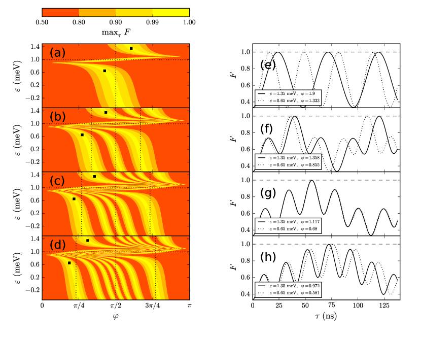
Figure F1: Fidelity $F$ for a broader range of the detuning $\varepsilon$ and the phase in the hopping matrix elements, $\varphi$; the parameters $U$, $h$, and $t$ are the same as in Fig. 2 of the main text. (a,b) $F$ maximized over the gate time $\tau$ (scale bar). We consider the first (a), second (b), third (c), and fourth (d) local maximum of $F$. The black squares indicates the parameters for the time-dependent plots in (e)-(h). The horizontal dotted lines in (a)-(d) represent $\varepsilon=\sqrt{U^{2}{-}h^{2}}$, and the vertical dotted lines belong to values of $\varphi$ being $\frac{\pi}{2}$ (a-d); $\frac{\pi}{3}$, $\frac{2\pi}{3}$ (b); $\arccos\frac{2}{3}$, $\pi-\arccos\frac{2}{3}$ (c); $\arccos\frac{3}{4}$, $\pi-\arccos\frac{3}{4}$ (d). Note that the Schrieffer-Wolff transformation breaks down close to $\varepsilon=U\pm h$.

By averaging the Fidelity $F$ over a Gaussian distribution of $\varepsilon$ while keeping the time from a maximization for a fixed value of $\varepsilon$ we can include the effect of quasi-static noise in our model. Fig. F2 shows that there are some regions of high fidelity which seem to be quite robust against quasi-static noise.

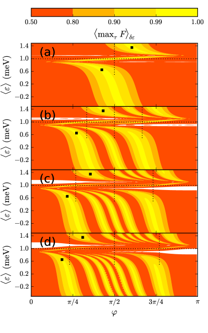
Figure F2: Fidelity in dependence of mean value of detuning $\langle\varepsilon\rangle$ and valley phase difference $\varphi$ for an average taken over a Gaussian distribution of $\varepsilon$ with standard deviation of $\sqrt{\langle\varepsilon^{2}\rangle-\langle\varepsilon\rangle^{2}}=8\mu$eV; this value was found in [S3] for a DQD in GaAs. While some small areas with $F>0.99$ from Fig. F1 are washed out the broader stripes of high fidelity “survive”.

We want to estimate the sensitivity of our ${\rm SWAP_{spin}}$ operation to electrical noise in comparison to the valley-free case. If no valley degeneracy is present the exchange interaction Hamiltonian is $-JP_{S}$ where $P_{S}$ is the projector on the spin singlet and, using the same assumptions as for our model, $J=4t^{2}U/(U^{2}-\varepsilon^{2})$. The sensitivity to electrical noise is in first order given by $\partial J/\partial\varepsilon$ [S4]. Therefore we compare $\partial J/\partial\varepsilon$ to the derivatives of the quantities $A$, $B$, $C$, and $\tilde{h}$ in $H_{\rm eff}$, see Eq. (1) of the main text and Eq. (B1) of this Supplemental Material. As the influence of the noise has to be considered relative to the gate time we plot in Fig. F3 the product of the derivative and the time when the first local maximum of the fidelity is reached. In Fig. F3 the hopping phase is $\varphi=1.333$. For the valley-free case this time is $\pi\hbar/J$. This is of course only a rough estimation, but at $\varepsilon\approx 0.65\,{\rm meV}$, which is the value where a very high fidelity is reached, the absolute values for the quantities from our $H_{\rm eff}$ are in the same order of magnitude as $(\partial J/\partial\varepsilon)\pi/J$. Thus we expect the noise sensitivity of our exchange-based interaction to be similar to the situation without valley degeneracy.

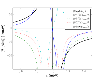
Figure F3: Derivatives of the quantities in the Hamiltonian in Eq. (1) of the main text (Eq. (B1) of this Supplemental Material) in comparison to $J=4t^{2}U/(U^{2}-\varepsilon^{2})$ for the spin-only exchange interaction. In order to have the comparison to the time needed for a ${\rm SWAP_{spin}}$ operation, we multiplied the derivatives with the time, when the fidelity of this quantum gate reaches first local maximum. The valley phase difference is given by $\varphi=1.333$.

It should be mentioned that for a fixed phase difference $\varphi$ we need to choose $\varepsilon$ such that the fidelity $F$ can be high whereas in the case without valley, $\varepsilon$ can be tuned in order to achieve low noise influence only worsen the gating time.

Furthermore noise can in principle also affect the gate via the tunneling parameter $t$, as it is done in Ref. [S5] we neglect this effect here.

VII D. Explicit sequences for quantum gates

In this section we give explicit sequences which show how single- and two-qubit gates can be applied in the two registers shown in Fig. 1 of the main text. In following we consider first the register Fig. 1 (a) and after that Fig. 1 (b). We introduce the notation ${\rm SWAP}_{sv}(m,m-1)$ for the $\rm SWAP_{\rm spin}\otimes\rm SWAP_{\rm valley}$ gate applied at the upper and the lower rows of the register between the dots at position $m$ and $m-1$. This gate is provided for dots with spin and valley degeneracy directly by exchange interaction [S6], i.e., in Fig. 1 (a) they can be applied for $m\leq 3$. Furthermore we denote the spin-only SWAP gate between the dots at position $m$ and $m-1$, applied again in the upper and the lower line of the register, by ${\rm SWAP}_{s}(m,m-1)$. This gate can be performed for the register Fig. 1 (a) for $m=2$ and for Fig. 1 (b) for any $m=2,3,4,\ldots$ The single qubit gates of the valley qubit in the $k$-th double quantum dot (DQD) in Fig. 1 (a) are realized by the four steps below:

1. Apply ${\rm SWAP}_{sv}(k,k-1),{\rm SWAP}_{sv}(k-1,k-2),\ldots,{\rm SWAP}_{sv}(3,2)$.

2. Apply ${\rm SWAP}_{s}(2,1)$.

3. Perform the single-qubit operation in DQD 2.

4. Repeat the second step and then the first in inverse order to bring the qubits back to position $k$.

The exchange interaction and a gradient in the valley splitting provides full control over two axis in Bloch sphere of the valley qubit and thus allow for the third step. Single-qubit operations with the $S$-$T_{0}$ spin triplet are done the same way using exchange and a gradient in the spin Zeeman field of DQD 1 within step 3 of the given procedure. For a two-qubit gate between the valley qubits of DQD $k$ and $m$ with $m>k$ the steps are as follows:

1. Apply ${\rm SWAP}_{sv}(k,k-1),{\rm SWAP}_{sv}(k-1,k-2),\ldots,{\rm SWAP}_{sv}(3,2)$ and ${\rm SWAP}_{sv}(m,m-1),{\rm SWAP}_{sv}(m-1,m-2),\ldots,{\rm SWAP}_{sv}(4,3)$.

2. Apply a SWAP gate between the spin and the valley qubit residing in DQD $k$. This is possible as any unitary operation is feasible in this subsystem.

3. Apply ${\rm SWAP}_{s}(2,1)$.

4. Apply ${\rm SWAP}_{sv}(3,2)$.

5. Apply ${\rm SWAP}_{s}(2,1)$.

6. Apply the two-qubit gate between the spin and the valley qubit in DQD 2, which are the former valley qubits of DQDs $k$ and $m$.

7. Return the qubits to their former position by reversing steps 1 to 5.

For a two-qubit gate between a spin and a valley qubit, step 2 is not necessary and between two spin qubits, step 2 exchanges the spin and valley qubits from the $m$-th instead of the $k$-th DQD.

We proved that universal quantum computing is possible in Fig. 1 (a), but should also ask how efficient our scheme is, in particular, whether it scales polynomially or not. To answer this question, we count the number of gates needed for a single-qubit operation each on the whole $2n-2$ qubits. We remember for a single gate on a qubit in the $k$-th DQD we need each $2(k-2)$ $\rm SWAP_{\rm spin}\otimes\rm SWAP_{\rm valley}$ gates for swapping the qubits to position 2 and back and two spin-only ${\rm SWAP}$ gates; all those gates are applied on the upper and the lower line of the register in parallel (so only counted once). Then for the qubits in the $k$-th DQD we need $2k-1$ quantum gates ($2k-4$ $\rm SWAP_{\rm spin}\otimes\rm SWAP_{\rm valley}$ gates, two spin-only ${\rm SWAP}$, and the single qubit gates, which we only count as one because they can be applied in parallel on the spin $S$-$T_{0}$ qubit in DQD 1 and on the valley $S$-$T_{0}$ qubit in DQD 2), see Fig. H1 for $k=4$. For applying single-qubit gates on each qubit in the register this means a total number of $\sum_{k=2}^{n}(2k-1)=O(n^{2})$ needed quantum gates.

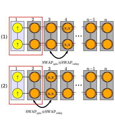
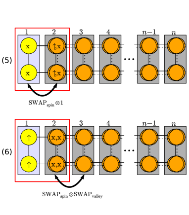
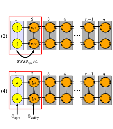
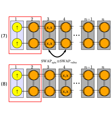
Figure H1: Performing single-qubit gates on the spin and the valley qubits in DQD 4 for register of Fig. 1 (a) of the main text. First, the qubits are moved to DQD 2 by ${\rm SWAP_{spin}}\otimes{\rm SWAP_{valley}}$ in step (1) and (2), then spin and valley qubit are separated in step (3), in step (4) the single-qubit gates are applied and finally by reversing (1-3) in steps (5-7) the qubits are moved back to their original position (8). In total $2\cdot 4-1=7$ gates are needed, note that all ${\rm SWAP}$ operations are done in parallel in the upper and the lower rows of the register in parallel and the single-qubit operations in step (4) can be performed in parallel in DQD 1 and DQD 2.

Now we consider Fig. 1 (b) of the main text and prove universality alike the register in Fig. 1 (a). The single-qubit gates are directly given by the alternating structure of the register. For the two-qubit gates between two valley qubits in DQD $k$ and $m>k$ the steps are as follows:

1. Swap the valley qubits with the spin qubit in DQD $m$.

2. Apply ${\rm SWAP}_{s}(m,m-1),{\rm SWAP}_{s}(m-1,m-2),\ldots,{\rm SWAP}_{s}(k+1,k)$.

3. Apply the two-qubit gate between the spin and the valley in DQD $m$.

4. Return the qubits to their former position by reversing step 2 and 1.

For a two-qubit gate between a spin and a valley qubit, step 1 is not necessary and between two spin qubits step 2 interchanges the spin and the valley from the $m$-th instead of the $k$-th qubit.

• G. Burkard and A. Imamoglu, Phys. Rev. B 74, 041307 (2006).

• L. H. Pedersen, N. M. Møller, and K. Mølmer, Phys. Lett. A 367, 47 (2007).

• O. E. Dial, M. D. Shulman, S. P. Harvey, H. Bluhm, V. Umansky, and A. Yacoby, Phys. Rev. Lett. 110, 146804 (2013)

• M. P. Wardrop and A. C. Doherty, Phys. Rev. B 90, 045418 (2014).

• D. Culcer, X. Hu, and S. Das Sarma Appl. Phys. Lett. 95, 073102 (2009).

• N. Rohling and G. Burkard, New J. Phys. 14, 083008 (2012).

References

- (1) D. Loss and D. P. DiVincenzo, Phys. Rev. A 57, 120 (1998).
- (2) For a recent review including both approaches, see C. Kloeffel and D. Loss, Annu. Rev. of Condens. Matter Phys. 4, 51 (2013).
- Petta et al. (2005) J. R. Petta, A. C. Johnson, J. M. Taylor, E. A. Laird, A. Yacoby, M. D. Lukin, C. M. Marcus, M. P. Hanson, and A. C. Gossard, Science 309, 2180 (2005).
- Foletti et al. (2009) S. Foletti, H. Bluhm, D. Mahalu, V. Umansky, and A. Yacoby, Nat. Phys. 5, 903 (2009).
- Levy (2002) J. Levy, Phys. Rev. Lett. 89, 147902 (2002).
- Benjamin (2001) S. C. Benjamin, Phys. Rev. A 64, 054303 (2001).
- Klinovaja et al. (2012) J. Klinovaja, D. Stepanenko, B. I. Halperin, and D. Loss, Phys. Rev. B 86, 085423 (2012).
- (8) R. Li, X. Hu, and J. Q. You, Phys. Rev. B 86, 205306 (2012).
- (9) J. M. Taylor, H.-A. Engel, W. Dur, A. Yacoby, C. M. Marcus, P. Zoller, and M. D. Lukin, Nat. Phys. 1, 177 (2005).
- (10) D. Stepanenko and G. Burkard, Phys. Rev. B 75, 085324 (2007).
- (11) G. Ramon, Phys. Rev. B 84, 155329 (2011).
- (12) I. van Weperen, B. D. Armstrong, E. A. Laird, J. Medford, C. M. Marcus, M. P. Hanson, and A. C. Gossard, Phys. Rev. Lett. 107, 030506 (2011).
- (13) M. D. Shulman, O. E. Dial, S. P. Harvey, H. Bluhm, V. Umansky, and A. Yacoby, Science 336, 202 (2012).
- (14) N. Rohling and G. Burkard, New J. Phys. 14, 083008 (2012).
- (15) For a recent review see F. A. Zwanenburg, A. S. Dzurak, A. Morello, M. Y. Simmons, L. C. L. Hollenberg, G. Klimeck, S. Rogge, S. N. Coppersmith, and M. A. Eriksson, Rev. Mod. Phys. 85, 961 (2013).
- (16) A. H. Castro Neto, F. Guinea, N. M. R. Peres, K. S. Novoselov, and A. K. Geim, Rev. Mod. Phys. 81, 109 (2009).
- (17) F. Kuemmeth, S. Ilani, D. C. Ralph, and P. L. McEuen, Nature (London) 452, 448 (2008).
- (18) M. Shayegan, E. P. De Poortere, O. Gunawan, Y. P. Shkolnikov, E. Tutuc, and K. Vakili, Phys. Status Solidi (b) 243, 3629 (2006).
- (19) D. Xiao, G.-B. Liu, W. Feng, X. Xu, and W. Yao, Phys. Rev. Lett. 108, 196802 (2012).
- (20) A. Kormányos, V. Zólyomi, N. D. Drummond, and G. Burkard, Phys. Rev. X 4, 011034 (2014).
- (21) G. Feher and E. A. Gere, Phys. Rev. 114, 1245 (1959).
- (22) A. M. Tyryshkin, S. Tojo, J. J. L. Morton, H. Riemann, N. V. Abrosimov, P. Becker, H.-J. Pohl, T. Schenkel, M. L. W. Thewalt, K. M. Itoh, and S. A. Lyon, Nat. Mater. 11, 143 (2012).
- (23) T. B. Boykin, G. Klimeck, M. A. Eriksson, M. Friesen, S. N. Coppersmith, P. von Allmen, F. Oyafuso, and S. Lee, Appl. Phys. Lett. 84, 115 (2004).
- (24) M. O. Nestoklon, L. E. Golub, and E. L. Ivchenko, Phys. Rev. B 73, 235334 (2006).
- (25) S. Chutia, S. N. Coppersmith, and M. Friesen, Phys. Rev. B 77, 193311 (2008).
- (26) A. L. Saraiva, M. J. Calderón, X. Hu, S. Das Sarma, and B. Koiller, Phys. Rev. B 80, 081305 (2009).
- (27) D. Culcer, L. Cywiński, Q. Li, X. Hu, and S. Das Sarma, Phys. Rev. B 82, 155312 (2010b).
- (28) A. L. Saraiva, B. Koiller, and M. Friesen, Phys. Rev. B 82, 245314 (2010).
- (29) A. L. Saraiva, M. J. Calderón, R. B. Capaz, X. Hu, S. Das Sarma, and B. Koiller, Phys. Rev. B 84, 155320 (2011).
- (30) A. Baena, A. L. Saraiva, B. Koiller, and M. J. Calderón, Phys. Rev. B 86, 035317 (2012).
- (31) D. W. Drumm, A. Budi, M. C. Per, S. P. Russo, and L. C. L. Hollenberg, Nanoscale Res. Lett. 8, 111 (2013).
- (32) M. De Michielis, E. Prati, M. Fanciulli, G. Fiori, and G. Iannaccone, Appl. Phys. Express 5, 124001 (2012).
- (33) J. K. Gamble, M. Friesen, S. N. Coppersmith, and X. Hu, Phys. Rev. B 86, 035302 (2012).
- (34) J. K. Gamble, M. A. Eriksson, S. N. Coppersmith, and M. Friesen, Phys. Rev. B 88, 035310 (2013).
- (35) C. Tahan and R. Joynt, Phys. Rev. B 89, 075302 (2014).
- (36) L. Jiang, C. H. Yang, Z. Pan, A. Rossi, A. S. Dzurak, and D. Culcer, Phys. Rev. B 88, 085311 (2013).
- (37) L. Zhang, J.-W. Luo, A. Saraiva, B. Koiller, and A. Zunger, Nat. Commun. 4, 2396 (2013).
- (38) A. Dusko, A. L. Saraiva, and B. Koiller, Phys. Rev. B 89, 205307 (2014).
- (39) M. Xiao, M. G. House, and H. W. Jiang, Appl. Phys. Lett. 97, 032103 (2010).
- (40) M. G. Borselli, R. S. Ross, A. A. Kiselev, E. T. Croke, K. S. Holabird, P. W. Deelman, L. D. Warren, I. Alvarado-Rodriguez, I. Milosavljevic, F. C. Ku, W. S. Wong, A. E. Schmitz, M. Sokolich, M. F. Gyure, and A. T. Hunter, Appl. Phys. Lett. 98, 123118 (2011a).
- (41) M. G. Borselli, K. Eng, E. T. Croke, B. M. Maune, B. Huang, R. S. Ross, A. A. Kiselev, P. W. Deelman, I. Alvarado-Rodriguez, A. E. Schmitz, M. Sokolich, K. S. Holabird, T. M. Hazard, M. F. Gyure, and A. T. Hunter, Appl. Phys. Lett. 99, 063109 (2011b).
- (42) W. H. Lim, C. H. Yang, F. A. Zwanenburg, and A. S. Dzurak, Nanotechnology 22, 335704 (2011).
- (43) C. B. Simmons, J. R. Prance, B. J. Van Bael, T. S. Koh, Z. Shi, D. E. Savage, M. G. Lagally, R. Joynt, M. Friesen, S. N. Coppersmith, and M. A. Eriksson, Phys. Rev. Lett. 106, 156804 (2011).
- (44) C. H. Yang, W. H. Lim, N. S. Lai, A. Rossi, A. Morello, and A. S. Dzurak, Phys. Rev. B 86, 115319 (2012).
- (45) C. H. Yang, A. Rossi, R. Ruskov, N. S. Lai, F. A. Mohiyaddin, S. Lee, C. Tahan, G. Klimeck, A. Morello, and A. S. Dzurak, Nat. Commun. 4, 2069 (2013).
- (46) K. Wang, C. Payette, Y. Dovzhenko, P. W. Deelman, and J. R. Petta, Phys. Rev. Lett. 111, 046801 (2013).
- (47) T. M. Kott, B. Hu, S. H. Brown, and B. E. Kane, Phys. Rev. B 89, 041107 (2014).
- (48) B. Roche, E. Dupont-Ferrier, B. Voisin, M. Cobian, X. Jehl, R. Wacquez, M. Vinet, Y.-M. Niquet, and M. Sanquer, Phys. Rev. Lett. 108, 206812 (2012).
- (49) M. Yuan, R. Joynt, Z. Yang, C. Tang, D. E. Savage, M. G. Lagally, M. A. Eriksson, and A. J. Rimberg, Phys. Rev. B 90, 035302 (2014).
- (50) G. Yamahata, T. Kodera, H. O. H. Churchill, K. Uchida, C. M. Marcus, and S. Oda, Phys. Rev. B 86, 115322 (2012).
- (51) X. Hao, R. Ruskov, M. Xiao, C. Tahan, and H. Jiang, Nat. Commun. 5, 3860 (2014).
- (52) S. Goswami, K. A. Slinker, M. Friesen, L. M. McGuire, J. L. Truitt, C. Tahan, L. J. Klein, J. O. Chu, P. M. Mooney, D. W. van der Weide, R. Joynt, S. N. Coppersmith, and M. A. Eriksson, Nature Phys. 3, 41 (2007).
- (53) M. A. Eriksson, M. Friesen, S. N. Coppersmith, R. Joynt, L. J. Klein, K. Slinker, C. Tahan, P. M. Mooney, J. O. Chu, and S. J. Koester, Quantum Inf. Process. 3, 133 (2004).
- (54) B. Trauzettel, D. V. Bulaev, D. Loss, and G. Burkard, Nat. Phys. 3, 192 (2007).
- (55) B. M. Maune, M. G. Borselli, B. Huang, T. D. Ladd, P. W. Deelman, K. S. Holabird, A. A. Kiselev, I. Alvarado-Rodriguez, R. S. Ross, A. E. Schmitz, M. Sokolich, C. A. Watson, M. F. Gyure, and A. T. Hunter, Nature (London) 481, 344 (2012).
- (56) A. Pályi and G. Burkard, Phys. Rev. Lett. 106, 086801 (2011).
- (57) G. Y. Wu, N.-Y. Lue, and L. Chang, Phys. Rev. B 84, 195463 (2011).
- (58) G. Y. Wu, N.-Y. Lue, and Y.-C. Chen, Phys. Rev. B 88, 125422 (2013).
- (59) D. Culcer, X. Hu, and S. Das Sarma, Phys. Rev. B 82, 205315 (2010a).
- (60) D. Culcer, A. L. Saraiva, B. Koiller, X. Hu, and S. Das Sarma, Phys. Rev. Lett. 108, 126804 (2012).
- (61) Y. Wu and D. Culcer, Phys. Rev. B 86, 035321 (2012).
- (62) \BibitemOpenK. I. Kugel and D. I. Khomskii, Zh. Eksp. Teor. Fiz 64, 1429 (1973).
- (63) B. E. Kane, Nature (London) 393, 133 (1998).
- (64) L. M. K. Vandersypen, R. Hanson, L. H. W. van Beveren, J. M. Elzerman, J. S. Greidanus, S. D. Franceschi, and L. P. Kouwenhoven, in Quantum Computing and Quantum Bits in Mesoscopic Systems (Kluwer Academic/Plenum, New York, 2003) arXiv:quant-ph/0207059.
- (65) P. Recher, J. Nilsson, G. Burkard, and B. Trauzettel, Phys. Rev. B 79, 085407 (2009).
- (66) G. Burkard and A. Imamoglu, Phys. Rev. B 74, 041307 (2006).
- (67) See Supplemental Material below, which includes Ref. wardrop_doherty , for details on the Schrieffer-Wolff transformation, the time evolution with the effective Hamiltonian including an analytical result for the phase in Eq. (3), numerical results for the fidelity at the th local maximum with , considerations on the influence of quasistatic noise, and explicit sequences for the quantum gates.
- (68) M. P. Wardrop and A. C. Doherty, Phys. Rev. B 90, 045418 (2014).
- (69) L. H. Pedersen, N. M. Møller, and K. Mølmer, Phys. Lett. A 367, 47 (2007).
- (70) O. E Dial, M. D. Shulman, S. P. Harvey, H. Bluhm, V. Umansky, and A. Yacoby, Phys. Rev. Lett. 110, 146804 (2013).
- (71) D. Culcer and N. M. Zimmerman, Appl. Phys. Lett. 102, 232108 (2013).
- (72) D. P. DiVincenzo, Phys. Rev. A 51, 1015 (1995).
- (73) T. Ando, A. B. Fowler, and F. Stern, Rev. Mod. Phys. 54, 437 (1982).
- (74) B. E. Kane, N. S. McAlpine, A. S. Dzurak, R. G. Clark, G. J. Milburn, H. B. Sun, and H. Wiseman, Phys. Rev. B 61, 2961 (2000).
- (75) C. Herring, Bell Syst. Tech. J. 34, 237 (1955).
- (76) C. Herring and E. Vogt, Phys. Rev. 101, 944 (1956).
- (77) C. G. Van de Walle and R. M. Martin, Phys. Rev. B 34, 5621 (1986).
- (78) R. People and J. C. Bean, Appl. Phys. Lett. 48, 538 (1986).
- (79) M. M. Rieger and P. Vogl, Phys. Rev. B 48, 14276 (1993).
- (80) F. Schäffler, Semicond. Sci. Technol. 12, 1515 (1997).
- (81) D. Culcer, X. Hu, and S. Das Sarma, Appl. Phys. Lett. 95, 073102 (2009).
- (82) N. S. Lai, W. H. Lim, C. H. Yang, F. A. Zwanenburg, W. A. Coish, F. Qassemi, A. Morello, and A. S. Dzurak, Sci. Rep. 1, 110 (2011).