WUB/14-02
ZU-TH 12/14
LPN14-057
Higgs production in bottom quark annihilation:
Transverse momentum distribution at NNLO+NNLL
Abstract
We present the inclusive transverse momentum distribution for Higgs bosons produced in bottom quark annihilation at the LHC. The results are obtained in the five-flavor scheme. The soft and collinear terms at small are resummed through NNLL accuracy and matched to the NNLO transverse momentum distribution at large . We find that the theoretical uncertainty, derived from a variation of the unphysical scales entering the calculation, is significantly reduced with respect to lower orders.
1 Introduction
In the Standard Model (SM), Higgs boson production proceeds predominantly through gluon fusion. The theoretical efforts that went into the precise prediction of the corresponding total cross section as well as kinematical distributions are enormous (see Refs.[1, 2, 3] for more information). Other processes such as associated or production, or weak boson fusion, receive their importance from their characteristic final state particles or kinematics which typically improve the signal-to-background ratio relative to gluon fusion.
Similar to production, the Higgs boson can also be produced in association with bottom quarks (). Until now, however, this process has been largely disregarded in SM Higgs searches and studies, even though its cross section is larger than for production [4], since the suppression by the smaller Yukawa coupling is overcompensated by the increased phase space. However, in searches for a SM Higgs boson, the experimental significance of the associated production with bottom quarks suffers heavily from the enormous QCD background.
In theories with an extended Higgs sector, such as the Two-Higgs-Doublet Model (2HDM) or the Minimal Supersymmetric SM (MSSM), the bottom Yukawa coupling can be enhanced relative to the SM so that can become the dominant Higgs production mechanism. Concerning the theoretical prediction for this process, mainly two complementary approaches have been pursued in the past. In the four-flavor scheme (4FS), the leading-order (LO) partonic processes are and , where . This approach is most suitable when the bottom quarks are considered as part of the signature. The theoretical prediction is available through next-to-LO (NLO) QCD in the 4FS[5, 6, 7].
In the five-flavor scheme (5FS) at LO, the final state bottom quarks are considered as part of the proton remnants, which are implicitly integrated over in the parton model. The LO process thus becomes , which needs to be convolved with appropriate -quark density functions. The process evaluated in the 5FS is thus also referred to as bottom quark annihilation. This approach is most suitable for the calculation of the component to inclusive Higgs production. Its advantage with respect to the 4FS in this case is that, on the one hand, logarithms of the form ( is the bottom quark mass, the Higgs mass) which arise from integrating over the collinear region of the final state bottom quark momenta, are implicitly resummed through DGLAP evolution. On the other hand, due to the much simpler structure of the LO process, its theoretical prediction can be obtained at higher perturbative order than for the 4FS. Indeed, the next-to-NLO (NNLO) result for the inclusive total cross section in the 5FS has been known for more than 10 years [8]. The theoretical uncertainty, derived from renormalization and factorization scale variation, is significantly smaller than in the 4FS, in particular, for Higgs masses above 200 GeV. Experimental analyses are currently based on a pragmatic combination of the NLO 4FS and the NNLO 5FS result, as suggested in Ref.[9].
With increasing luminosity, kinematical distributions of the Higgs boson will become more and more important for the clear identification of this particle and the search for possible deviations from the SM predictions. Among the simplest observables in this respect is the transverse momentum () distribution of the Higgs. Comparison to theoretical predictions will provide a handle to the precise nature of the Higgs couplings, for example to gluons [10, 11, 12], where the Higgs-gluon coupling is mediated through a quark loop. Similarly, the associated production of a Higgs with bottom quarks plays a central role to measure the Higgs-bottom Yukawa coupling, in particular in theories where this coupling is enhanced.
It is well known that fixed-order predictions of the spectrum break down for small values of . A proper theoretical description in this region can be obtained by a resummation of logarithmic terms in , leading to a reordering of the perturbative series. At this point, it is useful to clarify our notation for the perturbative orders of the distribution. In gluon fusion as well as in within the 5FS, the kinematics of the LO partonic process is , so that the distribution vanishes for . Quite often one therefore speaks of the “LO distribution” only when an additional parton is emitted which can balance a finite of the Higgs. In this paper, however, we will consistently associate the term “LO” with the process, so that in our notation, the LO distribution in gluon fusion and 5FS- is .
In gluon fusion, the distribution has been studied in great detail. The NNLO result in the heavy-top limit was presented long ago [13, 14]. Subleading top-mass effects were calculated in Ref.[15]. For the resummation in the small- region, various approaches have been pursued. In Ref.[16], a matching procedure between the resummed next-to-next-to-leading logarithmic (NNLL) terms and the NNLO distribution has been suggested which, when integrated over all , reproduces the total cross section at NNLO. Its application to the gluon fusion process was implemented in the program HqT [17, 16, 18], which calculates the NNLO+NNLL spectrum of the Higgs in the limit of an infinitely heavy top mass. The effects of exact top and bottom masses on the resummed transverse momentum distribution were studied at NLO+NLL in Ref.[19, 20].111A similar study was pursued in Ref.[21], which additionally discusses the mass effects on the cross section, based on the techniques presented in Ref.[22].
For , the NNLO spectrum of the Higgs for in the 5FS was obtained in Ref.[23, 24]. The jet- and -vetoed rate [25, 23], as well as the fully differential cross section [26] are also known up to NNLO. The special case of production was considered earlier in Ref.[27]. So far, resummation of the spectrum of the Higgs produced in bottom annihilation has been considered only at NLO+NLL [28]. In this paper, we present the first result of the resummed NNLO+NNLL transverse momentum distribution in the 5FS.
The remainder of the paper is organized as follows: In Section 2.1, we give a brief outline of the resummation formalism for the production of an uncolored final state. This section also defines the notation for the rest of the article. Section 2.2 describes the matching procedure to the fixed-order result. In Section 2.3, we present our result for the so-called hard coefficient which was the only missing ingredient for the calculation of the resummed distribution at NNLO+NNLL. Our numerical results are presented in Section 3, including a description of the consistency checks that have been performed on the implementation (Section 3.1), the default input parameters (Section 3.2), and finally the distributions (Section 3.3) for the LHC at a center-of-mass energy of 8 TeV (results for 13 TeV are presented in Appendix D). We analyze the dependence of the differential cross section on the unphysical scales and the parton distributions. Section 4 contains our conclusions. In Appendix C, we give complementary information on complex Mellin transforms of some transcendental functions, that appear in our calculation.
2 Transverse momentum resummation
2.1 Elements
For the following discussion, it will be convenient to consider the production of a general colorless particle of mass with transverse momentum in proton-proton collisions. The specialization to , where , will be done in Section 2.3.
If is significantly smaller than , large logarithms of arise in the distribution due to an incomplete cancellation of soft and collinear contributions. Since each order of perturbation theory introduces additional powers of these logarithms, the naïve perturbative expansion in is no longer valid as . However, factorization of soft and collinear radiation from the hard process allows us to resum the logarithms to all orders in . This factorization is observed when working in the so-called impact parameter () space, defined via the Fourier transformation222The momentum conservation relates to the transverse momenta of the outgoing partons which is factorized in space using .
| (1) |
implying that the limit corresponds to . Using rotational invariance around the beam axis, the angular integration can be performed, so that we may write the distribution in the form
| (2) |
with the Bessel function , , and the hadronic center-of-mass energy. By the superscript “(res)” in Eq. (2), we have already indicated that we are going to use this equation only for , where the logarithmically enhanced terms need to be resummed. The proper inclusion of terms will be described in Section 2.2. Here and in what follows, the superscript is attached to process specific quantities; we will set DY for the Drell-Yan production of a vector boson, for example, and for the process.
It is convenient to consider the Mellin transform with respect to the variable of the resummed cross section in space,
| (3) |
which can be written as[29, 31]333Throughout this paper, parameters that are not crucial for the discussion will be suppressed in function arguments.
| (4) |
where is called the Born factor and determines the parton level cross section at LO. Unless indicated otherwise, the renormalization and factorization scales have been set to . The sum runs over all relevant quark flavors and their charge conjugates, as well as gluons, (where ). It takes into account that, already at LO, different initial states can contribute.444For example, the LO DY process receives contributions from all light quark flavors. In the process though, only is relevant, and
| (5) |
where is the Higgs mass, the bottom quark mass, and GeV is the vacuum expectation value of the Higgs field. The function in Eq. (4) is the Mellin transform of the density function of parton in the proton, where is the momentum fraction and the momentum transfer. The numerical constant , with Euler’s constant , is introduced for convenience.
The perturbative expansion of the resummation coefficients is given by
| (6) |
where . The order at which these coefficients are taken into account in Eq. (4) determines the logarithmic accuracy of the resummed cross section; leading logarithmic (LL) means that all higher order coefficients except for are neglected, next-to-LL (NLL) requires , , , and , etc. The coefficients required for the process at next-to-NLL (NNLL) accuracy are given in Section 2.3.
The fact that the coefficients , , and in Eq. (4) are process independent (i.e., they do not carry a superscript ) assumes a common resummation scheme555See Ref.[16] for details. for all ( initiated, ) processes . The entire process dependence is then contained in the hard coefficient and the Born factor . In the following, we will work in the DY scheme, where through all orders of perturbation theory. All resummation coefficients are known in the DY scheme up to the order required in this paper (see Section 2.3), with the exception of whose evaluation through NNLO will also be presented in Section 2.3.
Evolving the parton densities from to in Eq. (4) (see Ref.[16]), one can define the partonic resummed cross section through
| (7) |
From a perturbative point of view, can be cast into the form
| (8) |
where denotes the logarithms that are being resummed in , and is an arbitrary resummation scale. While is formally independent of , truncation of the perturbative series will introduce a dependence on this scale which is, however, of higher order. The variation of the cross section with will be taken into account when estimating the theoretical uncertainty of our final result in Section 3.3. Note that the entire dependence, parametrized in terms of , is contained in the functions which are defined to vanish at . Their generic perturbative expansion through NNLO, expressed in terms of the resummation coefficients of Eq. (6), can be found in Ref.[16]. The hard-collinear function depends on the coefficients and of Eq. (4). For and (for , see Ref. [32])
| (9) |
where . The expression for for the process including the full scale dependence through NNLO is given in Eq. (29).
Recalling that the formalism discussed in this section is valid only in the small- region, it is convenient to replace [16]
| (10) |
in the resummed cross section, which will prove useful in the next section to suppress the impact of in the large- region without affecting the logarithmic accuracy under consideration. Note, however, that this replacement changes the dependence of , so that Eq. (8)—and therefore —becomes explicitely dependent. We will come back to this issue in the next section.
2.2 Matching with the large- region
In the previous section we recalled the formalism of transverse momentum resummation at small . In order to obtain a result that is valid for arbitrary values of , a matching to the distribution at high values of is required, which is predominantly given by the fixed-order result. We will follow the additive matching procedure of Ref.[16], where the resummed-matched result is obtained by subtracting from the fixed-order distribution the logarithms at at the same order in , and adding the resummed expression at the appropriate logarithmic accuracy :
| (11) |
The logarithmic terms are obtained from the perturbative expansion of Eq. (2). The matching condition is imposed by requiring
| (12) |
which defines the logarithmic accuracy needed at each perturbative order in and vice versa. Thus, at a given order in , it determines to which order the resummation coefficients of Eq. (6) are required. Note that the dependence of introduced by the replacement of Eq. (10) cancels up to higher orders in Eq. (11).
Integrating Eq. (2) (with ) over by using (or elementary properties of the Fourier transform) and , it directly follows that
| (13) |
where the convolution of two functions and is defined as
| (14) |
Needless to say, and in Eq. (13) denote the inverse Mellin transforms of and .
For the r.h.s. of Eq. (13), it is ; using Eq. (12), it is thus easy to see that the integral over is the same for and . One therefore obtains a unitarity constraint on the resummed-matched cross section which implies that the integral over reproduces the total cross section at fixed order:666Note that this line of argumentation assumes that terms propotional to are included in as well as (implying also that logarithms are actual plus-distributions). In the practical application of Eq. (11), however, these terms cancel and can be disregarded.
| (15) |
This relation will be used in Section 2.3 to determine the second-order coefficient of the hard function numerically, which is the only missing piece for carrying out the full NNLL resummation for the process in the 5FS.
2.3 Resummation coefficients and determination of
In the DY scheme, the resummation coefficients relevant for the process read
| (16) |
where , , , and is the number of active quark flavors; furthermore with Riemann’s function. and are actually resummation scheme independent. Through , their expressions have been known for some time [33, 34], while has recently been calculated in Ref.[35]. The coefficient was first obtained in Ref.[36].
The coefficients which arise in our calculation are of the form (), the index denotes the bottom quark, and . Of course, the respective coefficients for the charge conjugate partons are also implied in this notation. In space (i.e., inverse Mellin space), the first-order coefficients in the DY scheme read [36]
| (17) |
The off-diagonal NLO coefficients () are resummation scheme independent. The second-order coefficients can be found in Ref.[37].
Finally, we need to determine the hard coefficient for the bottom annihilation process in the DY scheme. At NLO, it can easily be deduced from the first-order coefficient in the DY scheme [36] and in the scheme [24],777A general result for as a function of the finite part of the one-loop corrections has also been known for some time [38]. leading to . On the other hand, we have calculated the NNLO term in two independent ways.
Numerical evaluation.
Using Eqs. (11), (13) and (15), one finds
| (18) |
where . Eq. (18) holds order by order in and for each channel888As usual, the individual partonic subprocesses (channels) are defined according to the factorization scheme. separately.
If we consider at , the only unknown in Eq. (18) is the hard coefficient , which appears as a constant in the hard-collinear function (see Eq. (29)). The full dependence of the latter is known from the functions in the DY scheme. Thus, we can simply fit using Eq. (18) without any approximations. The numerical result we obtain is
| (19) |
where the relatively big uncertainty is caused by the cancellation of several digits on the right-hand side of Eq. (18).
Analytic evaluation.
The evaluation of the hard coefficient requires the knowledge of the purely virtual amplitude for the process which was calculated through NNLO in Refs.[8, 39]. We give below the UV renormalized999Both and are renormalized in the scheme. In particular, we replace in the whole amplitude according to Eq. (6) of Ref.[39]. form factor in dimensions for , where here and in what follows, denotes the Higgs boson mass .
| (20) |
where
| (21) |
and
| (22) | ||||
with . All singular terms are contained in , while remains independent of singularities. Note, however, that also contains finite terms. The splitting has been done according to Ref.[40]. The hard coefficient in the hard scheme at is then obtained at each order in through [40]
| (23) |
Using the fact that scheme conversion is process independent, i.e.,
| (24) |
with an appropriate perturbative factor , and that , the conversion to the DY scheme is easily carried out using
| (25) |
where is the hard coefficient for the DY process in the hard scheme which is presented in Ref.[40]. In this way we find
| (26) |
This yields a numerical value of , which is in perfect agreement with Eq. (19). This serves as an important check of our calculation.
3 Outline of the calculation and results
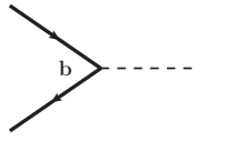
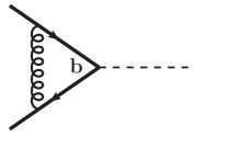
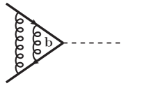
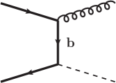
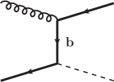
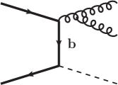
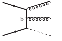
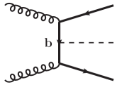
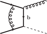
We are now ready to consider the resummed transverse momentum distribution of the Higgs boson produced via bottom quark annihilation through NNLO+NNLL. Exemplary Feynman diagrams that enter our calculation are shown in Appendix A. The LO diagram in Fig. 11 (a) determines the Born factor given in Eq. (5). The virtual one- and two-loop corrections (e.g. Fig. 11 (b) and (c)) govern the hard coefficient as outlined in Section 2.3. Fig. 12 shows a sample of real and mixed real-virtual diagrams that appear at NNLO for . Note that the various subprocesses enter the calculation at different orders. The initial state is the only subprocess present at LO. At NLO the contribution of the channel also has to be taken into account.101010We account all charge conjugated and switched initial states to the same subprocess. Thus, the channel includes , , and . The -, -, - and -initiated subprocesses () enter only at NNLO. The only subprocess which is finite at small transverse momenta and needs no resummation is the channel.
The calculation of the resummed-matched distribution of Eq. (11) requires the differential cross section111111The superscript = will be dropped in what follows. calculated in various approximations:
- •
- •
-
•
For the calculation of the resummed expression, , we use a modified version of the program HqT [17, 16, 18], which performs the transverse momentum resummation for gluon-induced Higgs production in the heavy-top limit. We extended its capabilities to also cover the resummation for quark-induced processes and implemented the resummation coefficients of the process.
3.1 Checks
Before presenting numerical results, we comment on various checks that we made on our calculation and outline our default input parameters. The analytic distribution at NNLO [24] has been checked numerically against the partonic Monte Carlo program for jet production at the same order of Refs.[23, 25], which in turn has been validated by various related calculations131313For more details see also Ref.[41].[27, 42, 43, 44, 45].
The small- behavior of the distribution needs to agree with the expansion of . We checked that the limit
| (27) |
holds to better than one per-mille in the interval GeV GeV. We also verified that this limit is independent of the resummation scale.
Furthermore, we used our implementation of to calculate a large number of sampling points in order to approximate the integral over . According to Eq. (13), the result has to yield the (analytically known) hard-collinear function , which we verified up to an accuracy of a few per-mille.141414More precisely, to verify Eq. (13) we used resummation scales significantly smaller than the mass of the Higgs to reduce the impact of resummation at high transverse momenta, because at very high ( GeV) the numerical convergence of our implementation of deteriorates. This is quite remarkable, considering the fact that the determination of includes the numerical transform from to space and from to space, as well as a fit of the parton distributions in Mellin space.
We also checked Eq. (15) for the resummed-matched cross section up to a numerical accuracy considerably better than one per-mille, using the analytical result for as the integral of . This was already expected from the agreement between Eq. (19) and the analytical result of Eq. (26) for mentioned above.
All these checks have been performed for various values of the resummation, factorization, and renormalization scale, separately at order and , and for the individual partonic subchannels.
At NLO+NLL, the spectrum of the Higgs in has already been studied in Ref.[28] within the formalism of Refs.[29, 30]. Although their approach—in particular, the matching procedure—differs from ours, the qualitative behavior of our curves is in fairly good agreement at this order. In particular, we find the same properties of the resummed-matched curve at high transverse momenta, which is nontrivial as will be shown in Section 3.3.
3.2 Input parameters
We present results for the LHC at and TeV center-of-mass energy. Our choice for the central factorization and renormalization scale is ; our default value for the resummation scale is . If not stated otherwise, all numbers are obtained with the MSTW2008 [46] PDF set, which implies that the input value for the strong coupling constant is taken as at NLO, and at NNLO. For comparison we also report results for the NNPDF2.3 and CT10 PDF sets, with their corresponding values. Since we are working in the 5FS, the bottom mass is set to zero throughout the calculation, except for the bottom-Higgs Yukawa coupling which we insert in the scheme at the scale , derived from the input value GeV.
All numbers are evaluated within the framework of the SM. Through appropriate rescaling of the bottom Yukawa coupling, they are obviously also applicable to neutral ( even and odd) Higgs production within the 2HDM and, according to the studies of Refs.[47, 48], even within the MSSM.
Sources of theoretical uncertainty and their impact on the numerical results will be studied in Section 3.3. As usual, the uncertainty due to the truncation of the perturbative series with respect to will be estimated from the dependence of the cross section on the unphysical scales and . Similarly, the effect of a finite logarithmic accuracy will be addressed by a variation of . Finally, we will investigate the uncertainty induced by the PDFs and the input value of .
3.3 Transverse momentum distribution up to NNLO+NNLL
In this section we present our results for the transverse momentum distribution of Higgs bosons produced in bottom quark annihilation. We study the impact of the newly evaluated terms at NNLO+NNLL by comparing them to NLO+NLL, both in absolute size and in their theoretical uncertainty.
|
 |
| (a) | (b) |
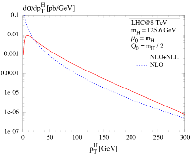
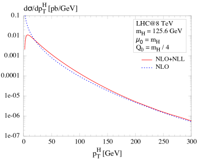
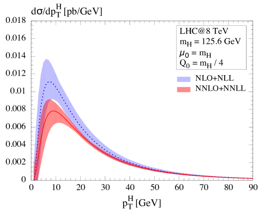
Fig. 1 shows the NLO+NLL together with the fixed-order NLO distribution for two values of the resummation scale : Fig. 1 (a) uses , which is the default value typically used in gluon fusion [16], while Fig. 1 (b) uses . Resummation aims at a valid description of the low- region and indeed, the divergence at of the fixed-order result is turned into a regular behavior. Due to higher-order effects, the fixed-order and the resummed-matched curve may also significantly differ at [28], as is also observed for gluon fusion [19, 21].151515A standard option in HqT [17, 16, 18], for example, is to use an intersection point between the fixed-order and the resummed-matched curve in order to switch from the latter to the former towards large . Fig. 1 shows that for bottom quark annihilation, this difference is significantly smaller for than for . This observation motivates us to use as the central resummation scale choice also at NNLO+NNLL in the following.161616We thank an anonymous referee for this suggestion. Nevertheless, for reference, we include results for in Appendix E.
|
 |
| (a) | (b) |
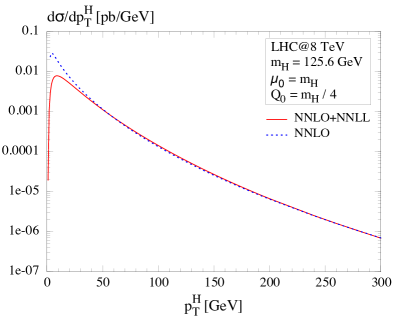
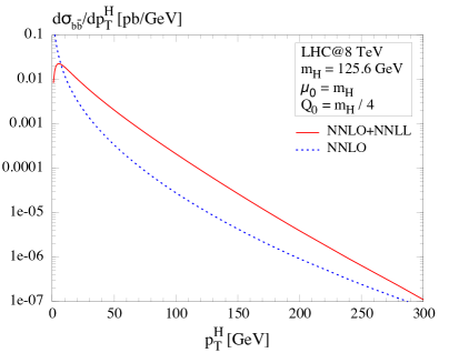
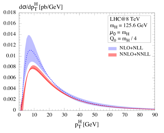
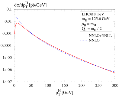
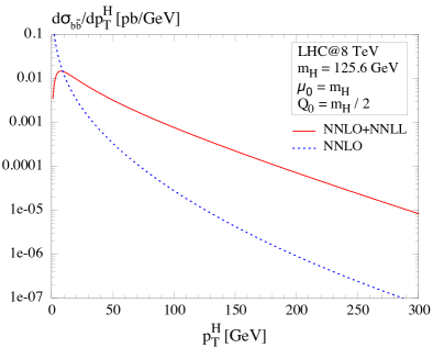
At NNLO+NNLL, we find that the agreement between the fixed-order and the resummed-matched curve is further improved with respect to NLO+NLL, see Fig. 2 (a). This confirms that the difference between these two results at is due to higher-order effects. For GeV, the resummed-matched curve is practically on top of the fixed-order curve. We note in passing that the agreement between the fixed-order and the resummed-matched curve results from nontrivial cancellations among the individual partonic subchannels. For example, considering only the channel, there are still large differences between the two curves, see Fig. 2 (b), which are, however, compensated by the other partonic channels. In conclusion, the NNLO+NNLL result is the first to combine the small and high- region in a satisfactory way. This indicates its importance to obtain a distribution valid at all transverse momenta.
|
 |
| (a) | (b) |
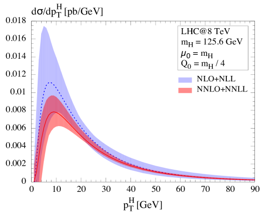
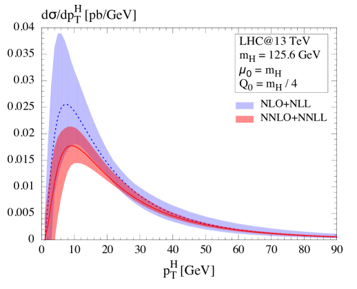
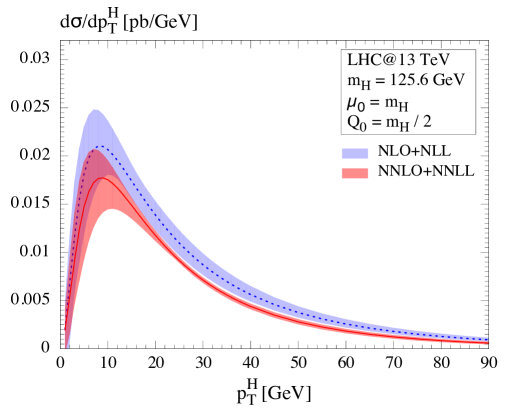
Let us now consider the effect of the higher orders on the dependence due to the renormalization and the factorization scale, while fixing the resummation scale at its default value, . The bands in Fig. 3 correspond to an independent variation of and in the range , while excluding the region where and . Comparing the red NNLO+NNLL with the blue NLO+NLL band, a considerable decrease of the scale uncertainties is only observed for GeV, while in the region where resummation is crucial the error bands have a similar size.
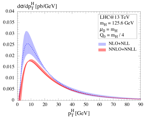
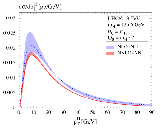
Including higher orders in the logarithmic accuracy, one also expects a reduction of the dependence of the distribution on the resummation scale. This is impressively confirmed in Fig. 4, which shows the cross sections at NLO+NLL and at NNLO+NNLL, where and are fixed at their default values (see Section 3.2). The bands are obtained by varying between and ; the lines correspond to . The variation of the cross section with respect to at NNLL is indeed significantly reduced with respect to NLL.
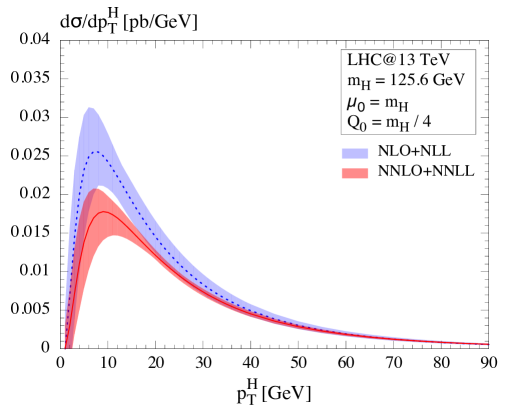
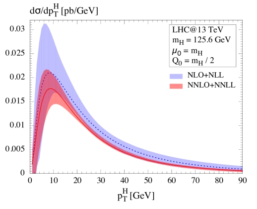
Finally, Fig. 5 shows the result for an independent variation of all three scales within and , where again we exclude the regions and . For all values of , one observes a reduction of the uncertainty of the resummed-matched NNLO+NNLL cross section with respect to the one at NLO+NLL. The relative uncertainty at the maximum amounts to % for the NNLL curve and at NLL.
The corresponding plots for TeV are shown in Appendix D, Fig. 15-13. Qualitatively, the above statements also apply here, only the absolute cross section is larger.
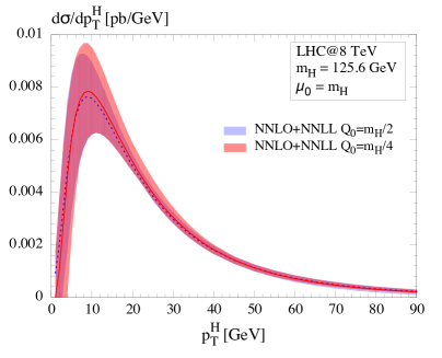
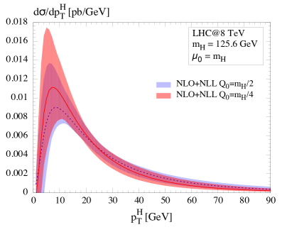
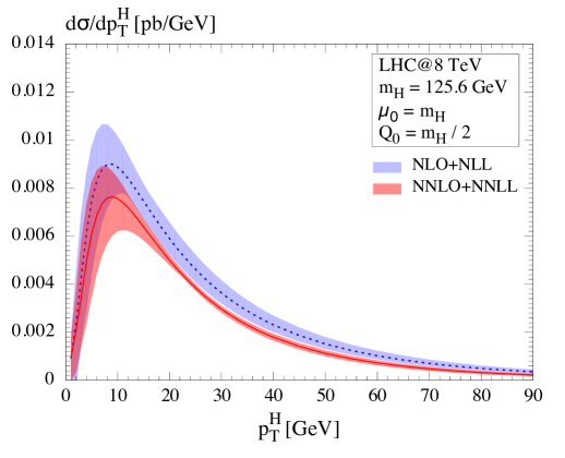
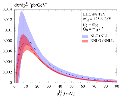
At this point, we would like to get back to the central choice of the resummation scale. As we have argued before, results in a good agreement in the high- tail of the resummed-matched and fixed-order distribution, particularly at NNLO+NNLL. Furthermore, at this order, the choice of only has a small impact on the distribution and the corresponding scale uncertainties at low . This is shown in Fig. 6 (a), which compares the curves for (blue, dotted line) and (red, solid line) at NNLO+NNLL. The bands correspond to the variation of all scales as described above. The height of the peak differs only by about 3% between the two choices. The corresponding curves at NLO+NLL show a significantly larger difference, which is about 23% at the peak, see Fig. 6 (b). Let us note again that, for further comparison, plots for are given in Appendix E, Fig. 16-20.
|
 |
| (a) | (b) |
![[Uncaptioned image]](/html/1403.7196/assets/x12.png)
![[Uncaptioned image]](/html/1403.7196/assets/x13.png)
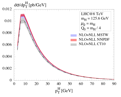
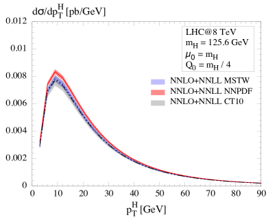
Finally, let us discuss the uncertainties arising from the PDF and choices. Besides the importance for our calculation, this study is particularly interesting regarding the treatment of the bottom densities of the various PDF groups, given the fact that the process in the 5FS is directly sensitive to the bottom densities. We consider three different PDF sets: MSTW2008, NNPDF2.3 and CT10. The combined PDF+ uncertainties are determined following the recommendations of the corresponding PDF groups [46, 49, 50]. In contrast to MSTW and CTEQ, there is no central PDF set for NNPDF, which is why the central value is calculated as the mean value of all considered PDF members.
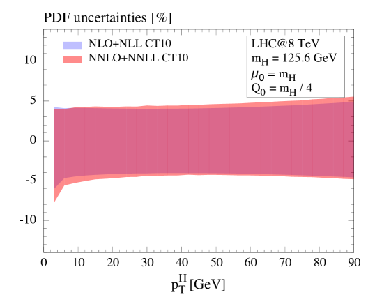
Fig. 7 compares the resummed-matched distributions obtained with the three PDF sets and their intrinsic uncertainties, for (a) NLO+NLL and (b) NNLO+NNLL accuracy. At NLO+NLL, the MSTW and NNPDF results are very consistent within their uncertainties, while the CTEQ band is right below the MSTW band. At NNLO+NNLL, on the other hand, the situation is the other way round: The bands of MSTW and CTEQ overlap, while the NNPDF band lies right on top of them. In both cases the biggest discrepancies are observed around the maximum of the distribution. This property may be due to the rather special role of the bottom densities which are not determined directly from experimental data, but are theoretically derived from the other parton densities and thus, are strongly dependent on their specific treatment in the different PDF groups. Furthermore, considering the relative uncertainties in Fig. 9 (MSTW), Fig. 9 (NNPDF) and Fig. 10 (CTEQ), we observe PDF+ uncertainties of similar size for the NLO and NNLO densities. This is expected since the PDF uncertainties arise only from the experimental input data. In fact, the NNLO uncertainties are slightly increased with respect to the NLO ones. In general the uncertainties of both cross sections NLO+NLL and NNLO+NNLL are rather small, %, % and % for MSTW, NNPDF and CTEQ, respectively.
The overall theoretical uncertainty on the cross section is clearly dominated by unphysical scales, in particular the factorization and renormalisation scale. It is therefore convenient to simply add the PDF+ and scale uncertainty in quadrature.
4 Conclusions
The transverse momentum distribution of Higgs bosons produced in bottom quark annihilation has been presented through NNLO+NNLL accuracy, following the method of Ref.[16]. For this purpose, we calculated the missing second-order hard coefficient both numerically and analytically. By choosing an appropriate resummation scale, we obtain a resummed-matched distribution that matches well to the fixed-order prediction at large already at NLO+NLL. At NNLO+NNLL, we observe excellent agreement between the resummed-matched and the fixed-order curve already above around 50 GeV. Our results therefore represent a precise prediction in the dominant region of low and intermediate values of transverse momenta.
Concerning the variation of the cross section with the unphysical scales, we observe a significant reduction when going from NLO+NLL to NNLO+NNLL. In fact, the extremely weak dependence of the NNLO+NNLL result on the resummation scale is remarkable. The PDF uncertainties are roughly of the same size at NLO+NLL and NNLO+NNLL, as it is expected from their purely experimental origin.
Our results should prove useful, in particular, in scenarios with enhanced bottom quark Yukawa coupling, such as supersymmetric or Two-Higgs-Doublet Models with large values of , but they may even be an important complement in the SM, especially once the statistics for Higgs events has improved. Not least of all, differential quantities in the process provide good physical observables to study various parametrizations and implementations of densities.
Acknowledgements.
We would like to thank Giancarlo Ferrera and Massimiliano Grazzini for enlightening discussions, and J. Blümlein for helpful communication. The work of A.T. was supported in part by the University of Torino, the Compagnia di San Paolo, contract ORTO11TPXK, and DFG, contract HA 2990/5-1. M.W. was supported by BMBF, contract 05H12PXE, and by the European Commission through the FP7 Marie Curie Initial Training Network “LHCPhenoNet” (PITN-GA-2010-264564).
Appendix Appendix A Feynman diagrams
|
 |
 |
|---|---|---|
| (a) | (b) | (c) |
 |
 |
 |
||
| (a) | (b) | (c) | ||
 |
 |
 |
||
| (d) | (e) | (f) |
Appendix Appendix B Hard-collinear coefficient with full scale dependence
In this appendix, we present expressions for the hard-collinear function to second order with complete scale dependence for the process:
| (28) | ||||
| (29) | ||||
where denotes the Higgs mass, is defined in Eq. (64) of Ref.[16], and denotes the Altrelli-Parisi splitting functions. Their expressions can be found in Ref.[51], for example. The quark mass anomalous dimension enters due to the fact that the Born factor is proportional to the square of the bottom quark mass (see Eq. (5)) which is normalized in the scheme:
| (30) |
while the power of at LO vanishes.
Appendix Appendix C Mellin transforms
Mellin transforms of several transcendental functions which appear in two-loop calculations are reported for integer in Ref.[52]. Ref.[53] gives a FORTRAN code that numerically approximates the analytic continuation of the moments of 25 basic functions171717The formula for in Eq. (30) of Ref.[53] contains a typo: The last term should be replaced by . We would like to thank J. Blümlein for confirmation. termed (see Section 3 of Ref.[53]). The resummation coefficients and can be expressed in terms of the moments of these 25 basic functions , and the analytic continuation of the single harmonic sums . Below, we give analytic expressions for Mellin transforms defined by
| (31) |
of some of the transcedental functions, true for complex , which appear in the coefficients of our calculation. The general definition of the harmonic sums is given by
| (32) |
which are defined, of course, only for integer and for . The analytic continuations are known for single sums and are expressed in terms of the digamma function and the polygamma functions . They are given by
| (33) | ||||
where
| (34) | ||||
and
| (35) | ||||
Appendix Appendix D Results for TeV
Appendix Appendix E Results for
In this appendix, we present the main results of the paper for a central resummation scale of .
|
 |
| (a) | (b) |

References
- [1] S. Dittmaier et al. [LHC Higgs Cross Section Working Group Collaboration], arXiv:1101.0593 [hep-ph].
- [2] S. Dittmaier et al. [LHC Higgs Cross Section Working Group Collaboration], arXiv:1201.3084 [hep-ph].
- [3] S. Heinemeyer et al. [LHC Higgs Cross Section Working Group Collaboration], arXiv:1307.1347 [hep-ph].
- [4] M. Spira, Fortsch. Phys. 46 (1998) 203 [hep-ph/9705337].
- [5] S. Dittmaier, M. Krämer, and M. Spira, Phys. Rev. D 70 (2004) 074010 [hep-ph/0309204].
- [6] S. Dawson, C.B. Jackson, L. Reina and D. Wackeroth, Mod. Phys. Lett. A 21 (2006) 89 [hep-ph/0508293].
- [7] S. Dawson, C.B. Jackson, L. Reina and D. Wackeroth, Phys. Rev. D 69 (2004) 074027 [hep-ph/0311067].
- [8] R.V. Harlander and W.B. Kilgore, Phys. Rev. D 68 (2003) 013001 [hep-ph/0304035].
- [9] R. Harlander, M. Krämer and M. Schumacher, arXiv:1112.3478 [hep-ph].
- [10] R.V. Harlander and T. Neumann, Phys. Rev. D 88 (2013) 074015 [arXiv:1308.2225 [hep-ph]].
- [11] A. Azatov and A. Paul, JHEP 1401 (2014) 014 [arXiv:1309.5273 [hep-ph]].
- [12] C. Grojean, E. Salvioni, M. Schlaffer and A. Weiler, arXiv:1312.3317 [hep-ph].
- [13] D. de Florian, M. Grazzini and Z. Kunszt, Phys. Rev. Lett. 82 (1999) 5209 [hep-ph/9902483].
- [14] C.J. Glosser and C.R. Schmidt, JHEP 0212 (2002) 016 [hep-ph/0209248].
- [15] R.V. Harlander, T. Neumann, K. J. Ozeren and M. Wiesemann, JHEP 1208 (2012) 139 [arXiv:1206.0157 [hep-ph]].
- [16] G. Bozzi, S. Catani, D. de Florian and M. Grazzini, Nucl. Phys. B 737 (2006) 73 [hep-ph/0508068].
- [17] G. Bozzi, S. Catani, D. de Florian and M. Grazzini, Phys. Lett. B 564 (2003) 65 [hep-ph/0302104].
- [18] D. de Florian, G. Ferrera, M. Grazzini and D. Tommasini, JHEP 1111 (2011) 064 [arXiv:1109.2109 [hep-ph]].
- [19] H. Mantler and M. Wiesemann, Eur. Phys. J. C 73 (2013) 2467 [arXiv:1210.8263 [hep-ph]].
- [20] M. Grazzini and H. Sargsyan, JHEP 1309 (2013) 129 [arXiv:1306.4581 [hep-ph]].
- [21] A. Banfi, P.F. Monni, G. Zanderighi, Quark masses in Higgs production with a jet veto, arXiv:1308.4634.
- [22] A. Banfi, P. F. Monni, G. P. Salam and G. Zanderighi, Phys. Rev. Lett. 109 (2012) 202001 [arXiv:1206.4998 [hep-ph]].
- [23] R.V. Harlander, K.J. Ozeren and M. Wiesemann, Phys. Lett. B 693 (2010) 269 [arXiv:1007.5411 [hep-ph]].
- [24] K.J. Ozeren, JHEP 1011 (2010) 084 [arXiv:1010.2977 [hep-ph]].
- [25] R. Harlander and M. Wiesemann, JHEP 1204 (2012) 066 [arXiv:1111.2182 [hep-ph]].
- [26] S. Bühler, F. Herzog, A. Lazopoulos and R. Müller, JHEP 1207 (2012) 115 [arXiv:1204.4415 [hep-ph]].
- [27] J.M. Campbell, R.K. Ellis, F. Maltoni and S. Willenbrock, Phys. Rev. D 67 (2003) 095002 [hep-ph/0204093].
- [28] A. Belyaev, P.M. Nadolsky and C.-P. Yuan, JHEP 0604 (2006) 004 [hep-ph/0509100].
- [29] J.C. Collins, D.E. Soper and G.F. Sterman, Nucl. Phys. B 250 (1985) 199.
- [30] P.M. Nadolsky, N. Kidonakis, F.I. Olness and C.-P. Yuan, Phys. Rev. D 67 (2003) 074015 [hep-ph/0210082].
- [31] S. Catani, D. de Florian and M. Grazzini, Nucl. Phys. B 596 (2001) 299 [hep-ph/0008184].
- [32] S. Catani and M. Grazzini, Nucl. Phys. B 845 (2011) 297 [arXiv:1011.3918 [hep-ph]].
- [33] J. Kodaira and L. Trentadue, Phys. Lett. B 112 (1982) 66.
- [34] S. Catani, E. D’Emilio and L. Trentadue, Phys. Lett. B 211 (1988) 335.
- [35] T. Becher and M. Neubert, Eur. Phys. J. C 71 (2011) 1665 [arXiv:1007.4005 [hep-ph]].
- [36] C.T.H. Davies and W. J. Stirling, Nucl. Phys. B 244 (1984) 337.
- [37] S. Catani, L. Cieri, D. de Florian, G. Ferrera and M. Grazzini, Eur. Phys. J. C 72 (2012) 2195 [arXiv:1209.0158 [hep-ph]].
- [38] D. de Florian and M. Grazzini, Nucl. Phys. B 616 (2001) 247 [hep-ph/0108273].
- [39] V. Ravindran, Nucl. Phys. B 752 (2006) 173 [hep-ph/0603041].
- [40] S. Catani, L. Cieri, D. de Florian, G. Ferrera and M. Grazzini, Nucl. Phys. B 881 (2014) 414 [arXiv:1311.1654 [hep-ph]].
- [41] M. Wiesemann, Nucl. Phys. Proc. Suppl. 234 (2013) 25 [arXiv:1211.0977 [hep-ph]].
- [42] S. Frixione and B.R. Webber, JHEP 0206 (2002) 029 [hep-ph/0204244].
- [43] R. Frederix, S. Frixione, F. Maltoni and T. Stelzer, JHEP 0910 (2009) 003 [arXiv:0908.4272 [hep-ph]].
- [44] S. Frixione, F. Stoeckli, P. Torrielli and B.R. Webber, JHEP 1101 (2011) 053 [arXiv:1010.0568 [hep-ph]].
- [45] V. Hirschi, R. Frederix, S. Frixione, M.V. Garzelli, F. Maltoni and R. Pittau, JHEP 1105 (2011) 044 [arXiv:1103.0621 [hep-ph]].
- [46] A.D. Martin, W.J. Stirling, R.S. Thorne and G. Watt, Eur. Phys. J. C 63 (2009) 189 [arXiv:0901.0002 [hep-ph]].
- [47] S. Dawson, C.B. Jackson and P. Jaiswal, Phys. Rev. D 83 (2011) 115007 [arXiv:1104.1631 [hep-ph]].
- [48] S. Dittmaier, M. Krämer, A. Mück and T. Schlüter, JHEP 0703 (2007) 114 [hep-ph/0611353].
- [49] R.D. Ball et al., Nucl. Phys. B 867 (2013) 244 [arXiv:1207.1303 [hep-ph]].
- [50] H.-L. Lai, M. Guzzi, J. Huston, Z. Li, P.M. Nadolsky, J. Pumplin and C.-P. Yuan, Phys. Rev. D 82 (2010) 074024 [arXiv:1007.2241 [hep-ph]].
- [51] R.K. Ellis and W. Vogelsang, hep-ph/9602356.
- [52] J. Blümlein and S. Kurth, Phys. Rev. D 60 (1999) 014018 [hep-ph/9810241].
- [53] J. Blümlein, Comput. Phys. Commun. 133 (2000) 76 [hep-ph/0003100].