Abstract

We prove the existence of globally attracting solutions of the viscous Burgers equation with periodic boundary conditions on the interval for some particular choices of viscosity and non-autonomous forcing. The attracting solution is periodic if the forcing is periodic. The method is general and can be applied to other similar partial differential equations. The proof is computer assisted.

Keywords:

viscous Burgers equation, periodic boundary conditions, non-autonomous forcing, attractor, rigorous numerics, interval arithmetic, logarithmic norm, computer assisted proof, self-consistent bounds

AMS classification:

Primary: 65M99, 35B40, 35B41. Secondary: 37B55, 65G40

1 Introduction

We present a method of proving the existence of globally attracting solutions for the viscous Burgers equation with periodic boundary conditions on the interval with a time-dependent forcing. The attracting solution is periodic, if the forcing is periodic. It is worth pointing out, that our method allows to obtain a globally attracting solution in case of non periodic forcings. Moreover, the method is general and should be applicable to other dissipative PDEs with periodic boundary conditions.

Let us begin with a short review of published results by both of the authors, which have been the foundation of our current research. In [C] a method of proving an existence of globally attracting steady-states for certain class of parabolic PDEs is presented. As an illustration of the method a detailed case study of the viscous Burgers equation is showed. The method can be summarized in three steps. First, construction of global absorbing sets, which are composed from regular functions, and such that they absorb any initial condition after a finite time. Second, establishing an existence of locally attracting steady-state. Third, absorbing sets are showed to be mapped into the fixed point’s local bassin of attraction by a rigorous numerical integration procedure. For the purpose of rigorous integration and establishing existence of an attracting fixed point we used a topological method of self-consistent bounds, developed in the series of articles [ZM, ZAKS, ZNS, Z2, Z3]. Now, let us shortly describe the innovation of the presented results. The current results generalize previous works as we deal with globally attracting orbits in the nonautonomous case. Establishing new results required from us extending the method of self-consistent bounds to the nonautonomous case, and deriving a new topological principle accompanied by an algorithm of proving existence of locally attracting solution defined on $\mathbb{R}$. To prove the attracting solution exists we verify that a time-shift map is contraction in certain space by construcing an interval enclosure of a so-called isolating segment for discrete semiprocess. Then we estimate the Lipschitz constant of the time-shift on the calculated enclosure. Observe that in [C, ZNS] the forcing was assumed to be constant in time, and in [ZM, ZAKS, Z2, Z3] the considered PDEs did not include any external forcing at all.

More specifically, in the present paper we present the case study of the initial value problem with periodic boundary conditions for the Burgers equation on the interval

$$u_{t}+u\cdot u_{x}-\nu u_{xx}=f(t,x),$$ (1)

First, as an example result we show

Theorem 1.1.

For any $\nu\in[2,2.1]$ and $f\in S_{1}$, where

$$S_{1}=\left\{x\mapsto 1.6\cos{2x}-2\sin{3x}+\sum_{k=1}^{3}{\beta_{k}(t)\sin{kx}+\gamma_{k}(t)\cos{kx}},\right.$$

$$\left.\beta_{k}(t),\ \gamma_{k}(t)\in\left[-0.03,0.03\right],\forall t\in\mathbb{R}\right\},$$

where $\beta_{k}(t),\ \gamma_{k}(t)$ are continuous, there exists a classical solution (periodic in time when $f$ is periodic in time) of (1), defined on $\mathbb{R}$, which attracts any initial data $u_{0}$ satisfying $u_{0}\in C^{4}$ and $\int_{0}^{2\pi}{u_{0}(x)\,dx}=\pi$. Moreover, the convergence towards attracting solution is exponential.

Theorem 1.1 in [C] about the existence of globally attracting fixed points when the forcing is time-independent is a particular case of Theorem 1.1 with $\beta_{k}(t)=\beta_{k},\ \gamma_{k}(t)=\gamma_{k}$ constant. As we show in Section 7 the computer assisted part of the proof of this theorem was in fact already accomplished during the proof of Thm. 1.1 in [C].

For the sake of demonstration, we state the next theorem for an explicitly given set of nonautonomous forcing functions with a particular dominant part. Our method is not restricted to this case, this particular nonautonomous dominant part is a result of setting some parameters in our algorithm. Our algorithm is capable to attempt to prove, in principle, any other case in which the dominant part is provided by explicit formulas.

Theorem 1.2.

For $\nu=2$ and $f\in S_{2}$, where

$$S_{2}=\left\{x\mapsto-0.6\sin(x)+0.7\cos(2x)+0.7\sin(2x)-0.8\cos(3x)-0.8\sin(3x)+\right.\\ \sin(t)\left[-0.6\cos(x)+0.7\cos(2x)+0.7\sin(2x)-0.8\cos(3x)-0.8\sin(3x)\right]+\\ \sum_{k=1}^{3}{\beta_{k}(t)\sin(kx)+\gamma_{k}(t)\cos(kx)},\\ \left.\beta_{k}(t),\,\gamma_{k}(t)\in\left[-5\cdot 10^{-5},5\cdot 10^{-5}\right],\ \forall t\in\mathbb{R}\right\},$$

where $\beta_{k}(t),\ \gamma_{k}(t)$ are continuous, there exists a classical solution (periodic in time when $f$ is periodic in time) of (1), defined on $\mathbb{R}$, which attracts any initial data $u_{0}$ satisfying $u_{0}\in C^{4}$ and $\int_{0}^{2\pi}{u_{0}(x)\,dx}=\pi$. Moreover, the convergence towards attracting solution is exponential.

In both theorems we are interested in classical solutions only. This is the reason, why we do not state the theorem for more general solutions.

The essential difference between Theorem 1.1 and Theorem 1.2 is that in Theorem 1.1 the non-autonomous part of the forcing (the time-dependent part) is a small perturbation of the autonomous part (the time-independent part). Whereas in Theorem 1.2 the norms of the autonomous, and the non-autonomous part of the forcing are of the same order of magnitude. Due to this fact the proofs of both theorems are based on the slightly different topological principle. In the proof of Thm. 1.1 we constructed a trapping isolating segment (a forward invariant set in the extended phases pace), which is time independent, while in the proof of Thm. 1.2 we constructed a trapping set (a forward invariant set) for the time shift along the orbits by $2\pi$ - the period of the dominant part of the non-autonomous forcing.

Let us comment on the role of the condition $\int_{0}^{2\pi}{u_{0}(x)\,dx}=\pi$ in Theorem 1.1 and Theorem 1.2. The condition $\int_{0}^{2\pi}{u_{0}(x)\,dx}\neq 0$, when compared to

$$\int_{0}^{2\pi}{u_{0}(x)\,dx}=0$$

makes the proof significantly harder numerically, due to the appearance of complex eigenvalues in the partial derivative of the vector field – see the numerical data (95) in Appendix A. Therefore for the illustration of our method we decided to take this more difficult case.

Similar results to ours can be found in literature. In [JKM] for any $\nu>0$ the authors established the existence of a globally attracting solution of (1) periodic in space and time, under assumption that forcing is periodic in time. Hence, in this respect, our results for the time-periodic forcing are significantly less general as we just consider particular cases of parameters. We believe that even in that case our approach is of some interest, as we are able to establish the exponential convergence rate to the attracting solution, while in [JKM] the authors clearly indicated that they cannot make such claim and they asked for the convergence rate in one of the stated problems [JKM, Problem 3(i)]. The method in [JKM] appears to be restricted to the scalar equation on one-dimensional domains, partially due to the use of the maximum principles. In [Si1] the author established a similar result for (1) with a time-periodic forcing proving also the exponential convergence to the attracting orbit in the periodic case. The technique used in [Si1] uses heavily the fact that the Cole-Hopf transformation transforms the Burgers equation to a linear parabolic equation. This significantly reduces the applicability of this approach to other PDEs.

The technique we use here is not restricted to some particular type of equation nor to the dimension one. We need some kind of ’energy’ decay as a global property of our dissipative PDEs and then if the system exhibits an attracting orbit, then we should, in principle, be able to prove it independently of the system dimensionality. Generally speaking, the applicability of our technique to a whole class of dPDEs follows from the method of self-consistent bounds properties, in [Z3] it is argued how the method of self-consistent bounds applies to PDEs with other nonlinearities, in [ZNS] the method is applied to the incompressible Navier-Stokes equations with an autonomous forcing. In [CZ], using the averaging principle, we established existence of globally attracting orbits, asymptotically for sufficiently large integral of the initial condition, for the 1D viscous Burgers and incompressible 2D Navier-Stokes equations with an nonautonomous forcing.

At the present state our technique strongly relies on the existence of good coordinates, the Fourier modes in the considered example. We hope that the further development of the rigorous numerics for dissipative PDEs based on other function bases, e.g. the finite elements, should allow to treat also different domains and boundary conditions in the near future.

1.1 Notation

Some notation: $\mathbb{R}_{+}=[0,\infty)$, $B(Z,\delta)$ a ball of size $\delta$ around the set $Z$. $B_{n}(z,r)$ is a ball in $\mathbb{R}^{n}$ with the center $z$ and radius $r$ with the distance function is known from the context.

We denote by $[x]$ an interval set $[x]\subset\mathbb{R}^{n}$, $[x]=\Pi_{k=1}^{n}[x^{-}_{k},x^{+}_{k}]$, $[x^{-}_{k},x^{+}_{k}]\subset\mathbb{R},\ -\infty<x_{k}^{-}\leq x_{k}^{+}<\infty$.

For a nonautonomous ODE

$$x^{\prime}=f(t,x),$$ (2)

where $x\in\mathbb{R}^{n}$ and $f$ is regular enough to guarantee uniqueness of the initial value problem $x(t_{0})=x_{0}$ for any $(t_{0},x_{0})$ for (2), by $\varphi(t_{0},t,x)=x(t_{0}+t)$, where $x(t)$ is a solution (2) with initial condition $x(t_{0})=x_{0}$. Obviously in each context it will be clearly stated what is the ordinary differential equation generating $\varphi$. We will sometimes refer to $\varphi$ as to the local process generated by (2).

2 Viscous Burgers equation with periodic boundary conditions on interval

The Burgers equation was proposed in [B] as a mathematical model of turbulence. There is a significant number of applications of the Burgers equation, see e.g. [Wh]. We consider the initial value problem for viscous Burgers equation on the interval with periodic boundary conditions and a non-autonomous forcing $F$, i.e.

$$u_{t}(t,x)+u(t,x)\cdot u_{x}(t,x)-\nu u_{xx}(t,x)=F(t,x),\quad t\in[t_{0},\infty),\ x\in\mathbb{R},$$ (3a)

$$u(t,x)=u(t,x+2\pi),\quad t\in[t_{0},\infty),\ x\in\mathbb{R},$$ (3b)

$$F(t,x)=F(t,x+2\pi),\quad t\in\mathbb{R},\ x\in\mathbb{R},$$ (3c)

$$u(t_{0},x)=u_{0}(x),\quad t_{0}\in\mathbb{R},\ x\in\mathbb{R},$$ (3d)

where $\nu>0$.

For the technical purposes we assume that

$$F(t,x)=f(x)+\widetilde{f}(t,x),$$ (4)

where $f$ and $\widetilde{f}$ are continuous and $2\pi$-periodic with respect to $x$ variable, and we define $F(t,x)$ for $t\in\mathbb{R}$. Later, we will put more restrictive conditions on $f$ and $\widetilde{f}$. In fact, $f$ will be given in an explicit form and for $\widetilde{f}$ we will demand some bounds.

We will use the Fourier series to study (3). Let

$$u(t,x)=\sum_{k\in\mathbb{Z}}a_{k}(t)\exp(ikx).$$ (5)

It is straightforward to write the problem (3) in the Fourier basis. We obtain the following infinite ladder of equations

$$\frac{da_{k}}{dt}=-i\frac{k}{2}\sum_{k_{1}\in\mathbb{Z}}{a_{k_{1}}\cdot a_{k-k_{1}}}+\lambda_{k}a_{k}+f_{k}+\widetilde{f}_{k}(t),\quad t\in[t_{0},\infty),\ k\in\mathbb{Z},$$ (6)

where

$$a_{k}(t_{0})=\frac{1}{2\pi}\int_{0}^{2\pi}{u_{0}(x)e^{-ikx}}\,dx,\quad k\in\mathbb{Z},$$ (7a)

$$f_{k}=\frac{1}{2\pi}\int_{0}^{2\pi}{f(x)e^{-ikx}}\,dx,\quad k\in\mathbb{Z},$$ (7b)

$$\widetilde{f}_{k}(t)=\frac{1}{2\pi}\int_{0}^{2\pi}{\widetilde{f}(t,x)e^{-ikx}}\,dx,\quad t\in\mathbb{R},\ k\in\mathbb{Z},$$ (7c)

$$\lambda_{k}=-\nu k^{2}.$$ (7d)

The reality of $u$, $f$ and $\widetilde{f}$ implies that for $k\in\mathbb{Z}$

$$a_{k}=\overline{a_{-k}},\quad f_{k}=\overline{f_{-k}},\quad\widetilde{f}_{k}(t)=\overline{\widetilde{f}_{-k}(t)}\text{ for }t\in\mathbb{R}.$$ (8)

In view of the above variables $\{a_{k}\}_{k\in\mathbb{Z}}$ are not independent, this motivates the following definition.

Definition 2.1.

In the space of sequences $\{a_{k}\}_{k\in\mathbb{Z}}$, where $a_{k}\in\mathbb{C}$, we will say that the sequence $\{a_{k}\}$ satisfies the reality condition iff

$$a_{k}=\overline{a_{-k}},\quad k\in\mathbb{Z}.$$ (9)

We will denote the set of sequences satisfying (9) by $R$. It is easy to see that $R$ is a vector space over the field $\mathbb{R}$.

We will assume that the initial condition for (6) satisfies

$$\frac{1}{2\pi}\int_{0}^{2\pi}{u_{0}(x)\,dx}=\alpha,\quad\text{for a fixed }\alpha\in\mathbb{R}.$$ (10)

We will require additionally that $f_{0}=0$, $\widetilde{f}_{0}(t)=0$ for $t\in\mathbb{R}$, and then (10) implies that $a_{0}(t)$ is constant, namely

$$a_{0}(t)=\alpha,\quad\forall t\geq t_{0}.$$ (11)

Definition 2.2.

For any given number $m>0$ the $m$-th Galerkin projection of (6) is

$$\frac{da_{k}}{dt}=-i\frac{k}{2}\sum_{\begin{subarray}{c}|k-k_{1}|\leq m\\ |k_{1}|\leq m\end{subarray}}{a_{k_{1}}\cdot a_{k-k_{1}}}+\lambda_{k}a_{k}+f_{k}+\widetilde{f}_{k}(t),\quad t\in[t_{0},\infty),\ |k|\leq m.$$ (12)

Here and further on with a slight abuse of notation we denote $m$-th Galerkin projection solution’s $k$-th mode by $a_{k}$, which is the same symbol as the $k$-th mode of the solution of the full system (6). Note that the condition (11) holds also for all Galerkin projections (12) as long as $f_{0}=0$, and $\widetilde{f}_{0}(t)=0$ for all $t\in\mathbb{R}$. Also observe that the reality condition (9) is invariant under all Galerkin projections (12), i.e. if $a_{k}(t_{0})=\overline{a_{-k}}(t_{0})$, then $a_{k}(t)=\overline{a_{-k}}(t)$ for all $t>t_{0}$ if the solution of (12) exists up to that time.

Definition 2.3.

Let ${\nmid}\cdot{\nmid}\colon\mathbb{R}\to\mathbb{R}$ be given by

$${\nmid}a{\nmid}:=\left\{\begin{array}[]{ll}|a|&\text{ if }a\neq 0,\\ 1&\text{ if }a=0.\end{array}\right.$$

Definition 2.4.

Let $H$ be the space $l_{2}(\mathbb{Z},\mathbb{C})$, i.e. $u\in H$ is a sequence $u:\mathbb{Z}\to\mathbb{C}$ such that $\sum_{k\in\mathbb{Z}}|u_{k}|^{2}<\infty$ over the coefficient field $\mathbb{R}$. The subspace $\widehat{H}\subset H$ is defined by

$$\widehat{H}:=\left\{\{a_{k}\}\in H\colon\text{there exists }0\leq C<\infty\text{ such that }|a_{k}|\leq\frac{C}{{\nmid}k{\nmid}^{4}}\text{ for }k\in\mathbb{Z}\right\}.$$

This space is equivalent to the space of sequences having the following weighted $l^{\infty}$ norm finite

$$\|\{a_{k}\}\|=\sup_{k\in\mathbb{Z}}{|k|^{4}|a_{k}|}$$

Definition 2.5.

Let the space $H^{\prime}$ be given by

$$H^{\prime}:=\widehat{H}\cap R.$$

Let us comment on Definitions 2.4 and 2.5. Despite the fact that we are dealing with complex sequences we use as the coefficient field the set of real numbers, because the reality condition is not compatible with the complex multiplication.

The choice of the particular subspace $H^{\prime}$ is motivated by the fact that the order of decay of coefficients $\{a_{k}\}\in H^{\prime}$ is sufficient for the uniform convergence of $\sum{a_{k}e^{ikx}}$ and every term appearing in (3a). Moreover, in Theorem 1.1 and Theorem 1.2 the attraction property is obtained within the class of $C^{4}$ functions due to the fact that the Fourier expansion of any i.c. $u_{0}\in C^{4}$ belongs to $H^{\prime}$. For the details see [C].

2.1 Absorbing set

The goal of this section is to establish for the existence of the forward invariant absorbing set for all Galerkin projections of (3), with good compactness properties. Here, we basically quote the results from [C] with some improvements.

Definition 2.6.

[C, Def. 4.6] Let $N_{0}\geq 0$, $\varphi_{n}$ be a local process induced by the $n$-th Galerkin projection of (6). A set $\mathcal{A}\subset H^{\prime}$ is called the absorbing set for large Galerkin projections of (6), if for any pair $(t_{0},u_{0})\in\mathbb{R}\times H^{\prime}$ there exists $t_{1}(u_{0})\geq 0$ such that for all $n>N_{0}$ and all $t_{0}\in\mathbb{R}$, $t\geq t(u_{0})$ holds $\varphi_{n}\left(t_{0},t,P_{n}u_{0}\right)\in P_{n}\mathcal{A}$. Moreover, $P_{n}\mathcal{A}$ is forward invariant for $\varphi_{n}$.

Our definition of the absorbing set differs from the standard one of bounded absorbing set, see for example [FMRT]. There it is stated for an abstract evolutionary equation and $t_{1}=t_{1}(B)$ has to be uniform for any bounded set $B$, whereas in our case, we state the definition for the more specific case of (sufficiently) large Galerkin projections of (6) and $t_{1}$ depends on point $u$, so we use the notion of point absorbing set. Observe that both mentioned concepts of absorbing sets are equivalent for a fixed $n$, but as we ask for uniformity in $n>N_{0}$ we use a weaker concept. Despite the fact that for the absorbing sets we construct in this work, $t_{1}$ can be chosen uniformly for each bounded set $B$, i.e. $t_{1}=t_{1}(B)$ we find this stronger requirement unnecessary.

Definition 2.7.

[C, Def. 3.1]

Energy of (6) is given by the formula

$$E(\{a_{k}\})=\sum_{k\in\mathbb{Z}}{|a_{k}|^{2}}.$$ (13)

Energy of (6) with $a_{0}$ excluded is given by the formula

$$\mathcal{E}(\{a_{k}\})=\sum_{k\in\mathbb{Z}\setminus\{0\}}{|a_{k}|^{2}}.$$ (14)

The theorem below is a main building block for the construction of the absorbing set.

Theorem 2.8.

Based on [C, Thm. 3.4] Assume that $F_{k}(t)=f_{k}+\widetilde{f}_{k}(t)$ for $t\in\mathbb{R}$ satisfies $F_{k}(t)=\overline{F_{-k}(t)}$, $F_{k}(t)=0$ for $|k|>J$, and $F_{0}(t)=0$. Let $\{a_{k}\}_{k\in\mathbb{Z}}\in H$, $s>0.5$, $E_{0}=\sup_{t\in\mathbb{R}}E\left(\left\{F_{k}(t)\right\}\right)\nu^{-2}<\infty$, $\widetilde{\mathcal{E}}>E_{0}$, $D=2^{s-\frac{1}{2}}+\frac{2^{s-1}}{\sqrt{2s-1}}$, $C>\sqrt{\widetilde{\mathcal{E}}}N^{s}$, $N>\max{\left\{J,\left(\frac{\sqrt{\widetilde{\mathcal{E}}}D}{\nu}\right)^{2}\right\}}$. Then

$$W(\widetilde{\mathcal{E}},N,C,s)=\left\{\{a_{k}\}\in R\ |\ \mathcal{E}(\{a_{k}\})\leq\widetilde{\mathcal{E}},\ |a_{k}|\leq\frac{C}{|k|^{s}}\right\}$$

is a trapping region (i.e. is forward invariant) for each Galerkin projection of (6).

The theorem below establishes the existence of a family of absorbing sets.

Theorem 2.9.

Based on [C, Lemma 4.7] Assume that $F_{k}(t)=f_{k}+\widetilde{f}_{k}(t)$ for $t\in\mathbb{R}$ satisfies $F_{k}(t)=\overline{F_{-k}(t)}$, $F_{k}(t)=0$ for $|k|>J$, and $F_{0}(t)=0$. Let $\varepsilon>0$, $E_{0}=\sup_{t\in\mathbb{R}}E\left(\left\{F_{k}(t)\right\}\right)\nu^{-2}<\infty$, $\widetilde{\mathcal{E}}>E_{0}$, $N$ is defined in Thm. 2.8. Put

$$s_{i} = i/2\text{ for }i\geq 2,$$

$$D_{i} = 2^{s_{i}-\frac{1}{2}}+\frac{2^{s_{i}-1}}{\sqrt{2s_{i}-1}}\text{ for }i\geq 2,$$

$$C_{2} = \varepsilon+\frac{1}{\nu}\left(\frac{1}{2}\widetilde{\mathcal{E}}+\sup_{\begin{subarray}{c}0<|k|\leq J\\ t\in\mathbb{R}\end{subarray}}{\frac{|f_{k}|+|\widetilde{f}_{k}(t)|}{|k|}}\right),$$ (15)

$$C_{i} = \varepsilon+\frac{1}{\nu}\left(C_{i-1}\sqrt{\widetilde{\mathcal{E}}}D_{i-1}+\sup_{\begin{subarray}{c}0<|k|\leq J\\ t\in\mathbb{R}\end{subarray}}{|k|^{s_{i}-2}\left(|f_{k}|+|\widetilde{f}_{k}(t)|\right)}\right)\text{ for }i>2,.$$ (16)

Then for all $i\geq 2$, and $\widetilde{C}_{i}>\sqrt{\widetilde{\mathcal{E}}}N^{s_{i}}$

$$H\supset\mathcal{W}_{i}\bigl{(}\widetilde{\mathcal{E}},C_{i},\varepsilon\bigr{)}:=\left\{\{a_{k}\}_{k\in\mathbb{Z}}\in R\ |\ \mathcal{E}(\{a_{k}\}_{k\in\mathbb{Z}})\leq\widetilde{\mathcal{E}},\ |a_{k}|\leq\frac{C_{i}}{|k|^{s_{i}}}\right\}\bigcap W(\widetilde{\mathcal{E}},N,\widetilde{C}_{i},s_{i}),$$

is an absorbing set for large Galerkin projections of (6).

The absorbing sets obtained in the above theorem, contrary to [C, Lemma 4.7], does not depend on $\alpha$ (10). As an consequence of Theorem 2.9, and some improvements of the algorithms presented in [C], we are not anymore constrained with large $\alpha$ values. We managed to prove some example theorems for cases with large $\alpha$ values, and the results are presented in Table 2.

The intersection with the trapping isolating segment $W$ is required to ensure the obtained set is forward invariant in time. The proof of Theorem 2.9 follows the scheme of the proof of [C, Lemma 4.7], however the following auxiliary lemma is required. Precisely, for the sake of proving Theorem 2.9, [C, Lemma 4.4] should be replaced by Lemma 2.10 below.

Lemma 2.10.

Assume that $F_{k}(t)=f_{k}+\widetilde{f}_{k}(t)$ for $t\in\mathbb{R}$ satisfies $F_{k}(t)=\overline{F_{-k}(t)}$, $F_{k}(t)=0$ for $|k|>J$, and $F_{0}(t)=0$. Let $H^{\prime}\supset W$ be trapping region (i.e. is forward invariant) for all Galerkin projections of (6), such that $P_{n}W\subset W$ for all $n$.

Assume that $C_{a}\geq 0$, $s_{a}>0.5$ are numbers such that

$$|a_{k}|\leq\frac{C_{a}}{|k|^{s_{a}}}\quad\text{ for }|k|>0\text{, and for all }a\in W.$$ (17)

Assume that $C_{\mathcal{N}}\geq 0$, $s_{\mathcal{N}}\geq s_{a}-1$ are numbers such that

$$\left|\mathcal{N}_{k}(a)\right|\leq\frac{C_{\mathcal{N}}}{|k|^{s_{\mathcal{N}}}}\quad\text{ for }|k|>0,\text{and for all }a\in W,$$

where

$$\mathcal{N}_{k}(a)=-i\frac{k}{2}\sum_{k_{1}\in\mathbb{Z}\setminus\{0,k\}}{a_{k_{1}}\cdot a_{k-k_{1}}}.$$ (18)

Then for any $\varepsilon>0$ there exists a finite time $\hat{t}\geq 0$ such that for all $l>0$ and $t\geq\hat{t}$, any $a(t_{0}+t)$ – the solution of $l$-th Galerkin projection of (6) such that $a(t_{0})\in P_{l}(W)$, satisfies

$$|a_{k}(t_{0}+t)|\leq\frac{C_{b}+\varepsilon}{|k|^{s_{b}}}\text{ for }0<|k|\leq l,$$ (19)

where

$$C_{b}=\left(C_{\mathcal{N}}+\sup_{\begin{subarray}{c}0<|k|\leq J\\ t\in\mathbb{R}\end{subarray}}{\left\{|F_{k}(t)||k|^{s_{\mathcal{N}}}\right\}}\right)/\nu,\quad s_{b}=s_{\mathcal{N}}+2.$$ (20)

Proof

Let us fix the Galerkin projection dimension $l>0$.

We consider the initial value problem for the l-th Galerkin projection of (6) with the initial condition $a(t_{0})=a_{0}\in P_{l}W\cap H^{\prime}$.

Using the reality condition (9) we obtain

$$\frac{d|a_{k}|^{2}}{dt}=\frac{da_{k}}{dt}\cdot a_{-k}+a_{k}\cdot\frac{da_{-k}}{dt}=\\ \left((\lambda_{k}-ika_{0})a_{k}+\mathcal{N}_{k}(a)+F_{k}(t)\right)a_{-k}+\left((\lambda_{k}+ika_{0})a_{-k}+\mathcal{N}_{-k}(a)+F_{-k}(t)\right)a_{k}=\\ 2\lambda_{k}|a_{k}|^{2}+\left(\mathcal{N}_{k}(a)+F_{k}(t)\right)a_{-k}+\left(\mathcal{N}_{-k}(a)+F_{-k}(t)\right)a_{k}.$$

From the reality condition for $a$, $\mathcal{N}$ and $F$ we obtain

$$\frac{d|a_{k}|^{2}}{dt}\leq 2\lambda_{k}|a_{k}|^{2}+2\left(\sup_{t\in\mathbb{R},u\in W}\left|\mathcal{N}_{-k}(u)+F_{-k}(t)\right|\right)\left|a_{k}\right|,$$

hence

$$\frac{d|a_{k}|}{dt}\leq\lambda_{k}|a_{k}|+\sup_{t\in\mathbb{R},u\in W}\left|\mathcal{N}_{-k}(u)+F_{-k}(t)\right|\quad\text{for}\ |a_{k}|>0.$$ (21)

Let

$$b_{k}=\sup_{t\in\mathbb{R},u\in W}\left|\mathcal{N}_{-k}(u)+F_{-k}(t)\right|/(-\lambda_{k}).$$ (22)

From (17), (18), (20) it follows that

$$b_{k}\leq\frac{C_{b}}{|k|^{s_{b}}},\quad|k|>0.$$ (23)

From (21) it follows that for $t\geq 0$ holds

$$\left|a_{k}(t_{0}+t)\right|\leq\left(\left|a_{k}(t_{0})\right|-b_{k}\right)e^{\lambda_{k}t}+b_{k},\text{ for }|k|>0.$$

From (23), and (17) we obtain for $t\geq 0$ and $|k|>0$

$$\left|a_{k}(t_{0}+t)\right|\leq\left(\frac{C_{a}}{|k|^{s_{a}}}-\frac{C_{b}}{|k|^{s_{b}}}\right)e^{\lambda_{k}t}+\frac{C_{b}}{|k|^{s_{b}}},\text{ for }|k|>0,$$

We would like to find $\hat{t}$ such that for $t\geq\hat{t}$ condition (19) is satisfied. It is easy to see that this is implied by the following inequality, which should be satisfied for $|k|\geq 1$

$$C_{a}|k|^{s_{b}-s_{a}}e^{\lambda_{k}t}\leq\epsilon.$$ (24)

Observe that $s_{b}>s_{a}$. Let us fix $n\in\mathbb{Z}_{+}$ such that $n>(s_{b}-s_{2})/2$. We have for $t>0$ and any $|k|\geq 1$

$$C_{a}|k|^{s_{b}-s_{a}}e^{\lambda_{k}t}=\frac{C_{a}|k|^{s_{b}-s_{a}}}{e^{\nu|k|^{2}t}}\leq\frac{C_{a}|k|^{s_{b}-s_{a}}}{(\frac{(\nu|k|^{2}t)^{n}}{n!})}\leq\frac{n!C_{a}}{\nu^{n}t^{n}}<\epsilon$$

for $t\geq\hat{t}$, $\hat{t}$ is large enough (independent of the dimension of the Galerkin projection, but depending on the set $W$). This finishes the proof of condition (19).

 

3 Topological theorems

In this section we state two topological theorems, which are used to obtain the attracting orbits. It is based on forward invariant sets (trapping regions) and the Brouwer theorem. We will use the terminology of the isolating segment introduced by R. Srzednicki (see [S1, SW]) and local processes.

3.1 Semiprocesses and nonautonomous differential equations

We start with introducing the notion of a local semiprocess which formalizes the notion of a continuous family of local forward trajectories in an extended phase–space.

Definition 3.1.

Assume that $X$ is a topological space and $\varphi:D\rightarrow X$ is a continuous mapping, $D\subset\mathbb{R}\times\mathbb{R}_{+}\times X$ is an open set. We will denote by $\varphi_{(\sigma,t)}$ the function $\varphi(\sigma,t,\cdot)$.

$\varphi$ is called a local semiprocess if the following conditions are satisfied

(S1)

$\forall\sigma\in\mathbb{R}$, $x\in X$ : $\{t\in\mathbb{R}_{+}:(\sigma,x,t)\in D\}$ is an interval,

(S2)

$\forall\sigma\in\mathbb{R}:\varphi_{(\sigma,0)}={\rm id}_{X}$

(S3)

$\forall\sigma\in\mathbb{R},\forall s,t\in\mathbb{R}_{+}:\varphi_{(\sigma,s+t)}=\varphi_{(\sigma+s,t)}\circ\varphi_{(\sigma,s)}$,

If $D=\mathbb{R}\times\mathbb{R}_{+}\times X$, we call $\varphi$ a (global) semiprocess. If $T$ is a positive number such that

(S4)

$\forall\sigma,t\in\mathbb{R}_{+}:\varphi_{(\sigma+T,t)}=\varphi_{(\sigma,t)}$

we call $\varphi$ a $T$-periodic local semiprocess.

A local semiprocess $\varphi$ on $X$ determines a local semiflow $\Phi$ on $\mathbb{R}\times X$ by the formula

$$\Phi_{t}(\sigma,x)=(\sigma+t,\varphi_{(\sigma,t)}(x)).$$ (25)

In the sequel we will often call the first coordinate in the extended phase space $\mathbb{R}\times X$ a time.

Let $\varphi$ be a local semiprocess and let $\Phi$ be a local semiflow associated to $\varphi$. It follows by $(S1)$ and $(S2)$ that for every $z=(\sigma,x)\in\mathbb{R}\times X$ there is an $0<\omega_{z}\leq+\infty$ such that $(\sigma,t,x)\in D$ if and only if $0\leq t<\omega_{z}$. Let $x\in X$, $\sigma\in\mathbb{R}$, then a left solution through $z=(\sigma,x)$ is a continuous map $v:(a,0]\rightarrow\mathbb{R}\times X$ for some $a\in[-\infty,0)$ such that:

(I)

$v(0)=z$,

(II)

for all $t\in(a,0]$ and $s>0$ with $s+t\leq 0$ it follows that $s<\omega_{v(t)}$ and $\Phi_{s}(v(t))=v(t+s)$.

If $a=-\infty$ then we call $v$ a full left solution. We can extend a left solution through $z$ onto $(a,0]\cup[0,\omega_{z})$ by setting $v(t)=\Phi_{t}((\sigma,x))$ for $0\leq t<\omega_{z}$, to obtain a solution through $z$. If $a=-\infty$ and $\omega_{z}=+\infty$, $v$ is called a full solution. If for each $x\in X$ $\omega_{x}=\infty$, then we will say that $\Phi$ is a global semiprocess.

Remark 3.2.

The differential equation

$$\dot{x}=f(t,x)$$ (26)

such that $f$ is regular enough to guarantee the uniqueness for the solutions of the Cauchy problems associated to (26) generates a local process as follows: for $x(t_{0},x_{0};\cdot)$ the solution of (26) such that $x(t_{0},x_{0};t_{0})=x_{0}$ we put

$$\varphi_{(t_{0},\tau)}(x_{0})=x(t_{0},x_{0};t_{0}+\tau).$$ (27)

If $f$ is $T$-periodic with respect to $t$ then $\varphi$ is a $T$-periodic local process. In order to determine all $T$-periodic solutions of equation (26) it suffices to look for fixed points of $\varphi_{(0,T)}$.

3.2 Trapping isolating segments

We use the following notation: by $\pi_{1}:\mathbb{R}\times X\rightarrow\mathbb{R}$ and $\pi_{2}:\mathbb{R}\times X\rightarrow X$ we denote the projections and for a subset $Z\subset\mathbb{R}\times X$ and $t\in\mathbb{R}$ we put

$$Z_{t}=\{x\in X:(t,x)\in Z\}.$$

Now we are going to state the definition of the trapping isolating segment, which is a modification of the notions of $T$-periodic isolating segment and periodic isolating segment over $[0,T]$ from [S1, SW].

Definition 3.3.

We will say that a set $Z\subset{\mathbb{R}}\times X$ is $T$–periodic, iff $Z_{T+t}=Z_{t}$ for every $t\in{\mathbb{R}}$.

We remark that according to the following definition $W(\widetilde{\mathcal{E}},N,C,s)$ from Theorem 2.8 is a trapping isolating segment.

Definition 3.4.

Let $W\subset{\mathbb{R}}\times X$. We call $W$ a trapping isolating segment for the global semiprocess $\varphi$ if:

(i)

$W\cap([t_{1},t_{2}]\times X)$ is a compact set for any $t_{1},t_{2}\in\mathbb{R}$

(ii)

for every $\sigma\in\mathbb{R}$, $x\in\partial W_{\sigma}$ there exists $\delta>0$ such that for all $t\in(0,\delta)$ $\varphi_{(\sigma,t)}(x)\in{\rm int}W_{\sigma+t}$.

Further we will need a notion of the trapping isolating segment for a differential inclusion

$$x^{\prime}(t)\in f(t,x(t))+[\delta],$$ (28)

where $x(t)\in\mathbb{R}^{n}$ and $[\delta]\subset\mathbb{R}^{n}$.

Definition 3.5.

Let $f$ be $C^{1}$ with respect to $x$, $\frac{\partial f}{\partial x}$ and $f$ be continuous with respect to $(t,x)$. We will say that $W\subset{\mathbb{R}}\times\mathbb{R}^{n}$ is a trapping isolating segment for (28) iff for any function $g:\mathbb{R}\times\mathbb{R}^{n}\to\mathbb{R}^{n}$, $C^{1}$ with respect to $x$, $\frac{\partial g}{\partial x}$ and $g$ continuous with respect to $(t,x)$, such that $g(t,x)\in[\delta]$, the set $Z$ is a trapping isolating segment for the semiprocess induced by

$$x^{\prime}(t)=f(t,x(t))+g(t,x(t)).$$ (29)

Theorem 3.6.

Assume that $W$ is a T-periodic trapping isolating segment for $T$-periodic global semiprocess $\varphi$ and $W_{0}$ is homeomorphic to $\overline{B}_{n}(0,1)$.

Then $W$ contains a $T$-periodic orbit.

Proof: Let $P$ be the map given by the time shift by $T$. $P$ is defined on $W_{0}$ and we have $P(W_{0})\subset W_{0}$. The Brouwer theorem implies the existence of $x\in W_{0}$, such that $P(x)=x$, which give rise to a $T$-periodic orbit.  

Theorem 3.7.

Assume $W$ is a trapping isolating segment for a global semiprocess $\varphi$ induced by a non-autonomous ODE

$$x^{\prime}=f(t,x),\quad f\in C^{1}(\mathbb{R}\times\mathbb{R}^{n},\mathbb{R}^{n}).$$ (30)

Then there exists $x\in W_{0}$, such that there exists a full orbit (forward and backward) through $x$ contained in $W$.

Proof: Each forward orbit starting from $W_{0}$ is contained in $W$. Therefore it is enough to prove the existence of full backward orbit in $W$.

It is easy to see that for any $l\in\mathbb{N}$ there exists $v_{l}:[-l,0]\to\mathbb{R}^{n}$ an orbit of our semiprocess contained in $W$.

We would like to show that we can chose a subsequence $\{u_{l_{k}}\}$ such that $u_{n_{l}}$ is converging locally uniformly on $(-\infty,0]$ to some full backward orbit $v$.

Let us fix any $k\in\mathbb{N}$. Observe that for $l>k$ $v_{l}$ is defined on $[-k,0]$ and are contained in $W\cap([-l,0]\times\mathbb{R}^{n})$, which is a compact set. Therefore there exists $M>0$ such that

$$|f(t,x)|\leq M,\qquad(t,x)\in W\cap([-k,0]\times\mathbb{R}^{n}).$$ (31)

Therefore

$$|v_{l}^{\prime}(t)|\leq M,\quad t\in[-k,0].$$ (32)

This shows that functions $\{v_{l}:[-k,0]\to\mathbb{R}^{n}\}$ are equicontinuous and contained in a bounded set $\pi_{x}(W\cap([-l,0]\times\mathbb{R}^{n})))$. It follows from the Ascoli-Arzela Theorem that we can chose subsequence $\{v_{l_{m}}\}$ which is uniformly converging on $[-k,0]$ to some continuous function $\overline{v}_{k}:[-k,0]\to\mathbb{R}^{n}$, which is an orbit of the semiprocess.

Now let us consider the following procedure: assume that we have a subsequence of solutions $v_{l_{i}}$ converging uniformly to $\overline{v}_{k}:[-k,0]\to\mathbb{R}^{n}$. From that sequence we can chose a subsequence which will be uniformly converging to $\overline{v}_{2k}:[-2k,0]\to\mathbb{R}^{n}$ and then we find a subsequence converging on $[-2^{2}k,0]$ to $\overline{v}_{2^{2}k}$ and so on. From all these nested subsequences $\{u_{l_{i}}\}$ by choosing diagonal elements $\{u_{l_{k}}\}$ we obtain a sequence, which is converging uniformly on each compact interval $[-k,0]$ to $\overline{v}$, such that $\overline{v}(t)=\overline{v}_{k}(t)$ for $t\in[-k,0]$. From the continuity of $\varphi$ it follows easily that $\overline{v}$ is a full backward orbit of $\varphi$. Obviously, $\overline{v}$ is contained in $W$.  

3.3 Discrete semiprocesses - iterations of maps

Definition 3.8.

Assume that we have an indexed family of continuous maps $\{f_{i}:\mathbb{R}^{n}\to\mathbb{R}^{n}\}_{i\in\mathbb{Z}}$. We define a map $\varphi:\mathbb{Z}\times\mathbb{Z}_{+}\times\mathbb{R}^{n}\to\mathbb{R}^{n}$ by

$$\varphi(i_{0},i,x)=\begin{cases}x&\text{if $i=0$},\\ f_{i_{0}+i-1}\circ\cdots f_{i_{0}+1}\circ f_{i_{0}}(x)&\text{otherwise}.\end{cases}$$ (33)

$\varphi$ we will be called a discrete semiprocess.

For $T\in\mathbb{Z}_{+}$ we say that $\varphi$ is $T$-periodic, if $f_{i+T}=f_{i}$ for all $i\in\mathbb{Z}$.

Analogously with the continuous case define the notion of the forward and backward orbit for a discrete semiprocess.

Definition 3.9.

Consider a set $W=\Pi_{k\in\mathbb{Z}}W_{k}$. It will be called a trapping isolating segment for the discrete semiprocess $\varphi$ if the following conditions are satisfied

(i)

$W_{k}$ is a compact set for any $k\in\mathbb{Z}$

(ii)

for every $k\in\mathbb{Z}$

$$\varphi(k,1,W_{k})\subset{\rm int}W_{k+1}.$$ (34)

For $T\in\mathbb{Z}_{+}$ we say that $W$ is $T$-periodic if $W_{k}=W_{T+k}$ for all $k\in\mathbb{Z}$.

We now establish discrete versions of theorems from Section 3.2.

Theorem 3.10.

Assume that $W$ is a T-periodic trapping isolating segment for a discrete $T$-periodic semiprocess $\varphi$ and $W_{0}$ is homeomorphic to $\overline{B}_{n}(0,1)$.

Then $W$ contains a $T$-periodic orbit.

The proof is the same as in the continuous case and will be omitted.

Theorem 3.11.

Assume $W$ is a trapping isolating segment for a discrete semiprocess $\varphi$.

Then there exist $x\in W_{0}$ and a full orbit (forward and backward) through $x$ contained in $W$.

The proof of this theorem uses the same idea as the proof of Theorem 3.7, but in the discrete case there is no need for the equicontinuity and the Ascoli-Arzela theorem.

4 The bounds for the Lipschitz constant for the time evolution of dissipative PDEs

4.1 Basic theorem on logarithmic norms and ODEs

Consider now the differential equation

$$x^{\prime}=f(t,x),$$ (35)

where $f$ and $\frac{\partial f}{\partial x}$ are is continuous.

By $\|x\|$ we denote a fixed arbitrary norm in $\mathbb{R}^{n}$. Let $\mu:\mathbb{R}^{n\times n}\to\mathbb{R}$ be the logarithmic norm of $A$ induced by norm $\|\cdot\|$, which was introduced independently by Dahlquist [D] and Lozinskii [L] (see also [HNW, KZ] and references given there)

$$\mu(A)=\lim_{h\to 0^{+}}\frac{\|1+hA\|-1}{h}.$$ (36)

Observe that $\mu(A)$ is not a norm, as it can be negative.

It was introduced, because gives us the bound for the Lipschitz constant of the the time shift by $h>0$ of the flow for trajectories contained in a convex compact set $W$ for $t\in[t_{0},t_{0}+h]$ in the form

$$L=\exp\left(h\max_{(t,x)\in[t_{0},t_{0}+h]\times W}\mu\left(\frac{\partial f}{\partial x}(t,x)\right)\right).$$ (37)

Observe that might to be less than one for attracting orbits (because the logarithmic norm can be negative). This should be contrasted with a more standard bound coming from the Gronwall inequality in the form

$$L=\exp\left(h\max_{(t,x)\in[t_{0},t_{0}+h]\times W}\left\|\frac{\partial f}{\partial x}(t,x)\right\|\right),$$ (38)

which never can be less than one.

A good illustration of the above phenomenon is a linear 1D equation

$$x^{\prime}=-x=f(t,x).$$

In this case we have the norm $\|x\|=|x|$. Since $\frac{\partial f}{\partial x}=[-1]$, so $\mu\left(\frac{\partial f}{\partial x}\right)=-1<0$ and we obtain a correct bound for the Lipschitz constant, $L$, of the time shift by $h>0$ given by

$$L=e^{-h}.$$ (39)

Depending on the norm $\|\cdot\|$ the formula for $\mu(A)$ differ. Let us list it for several popular norms

• for euclidian norm,

  $$\mu(A)=\max_{\lambda}\left\{\lambda\in\sigma\left(\frac{A+A^{T}}{2}\right)\right\},$$ (40)

  where $\sigma(M)$ is the spectrum of the matrix $M\in\mathbb{R}^{n\times n}$,

• for $\|x\|_{\infty}:=\max_{i=1,\dots,n}|x_{i}|$,

  $$\mu(A)=a_{ii}-\sum_{j,j\neq i}|a_{ij}|,$$ (41)

• for $\|x\|_{1}:=\sum_{i}|x_{i}|$,

  $$\mu(A)=a_{ii}-\sum_{j,j\neq i}|a_{ji}|.$$ (42)

In our work with attracting orbits we will always try to change coordinates so that the diagonal of $\frac{\partial f}{\partial x}$ dominates and has only negative entries. In this way we obtain that the logarithmic norm is negative (see formulas (40,41,42) ).

The following theorem is a precise statement on how to obtain the Lipschitz constant for the flow using the logarithmic norm. It was proved in [HNW, Th. I.10.6] (we use a different notation ).

Theorem 4.1.

Let $y:[t_{0},t_{0}+T]\to\mathbb{R}^{n}$ be a continuous piecewise $C^{1}$ function and $x:[t_{0},t_{0}+T]\to\mathbb{R}^{n}$ be a solution of (35).

Suppose that the following estimates hold:

$$\mu\left(\frac{\partial f}{\partial x}(t,\eta)\right) \leq l(t),\quad\mbox{ for $\eta\in[y(t),x(t)]$}$$

$$\left\|\partial_{+}y(t)-f(t,y(t))\right\| \leq \delta(t).$$

where $\partial_{+}y(t)=\lim_{h\to 0^{+}}\frac{y(t+h)-y(t)}{h}$, i.e. it is the right derivative of $y$ at $t$.

Then for $t>t_{0}$ holds

$$\|x(t)-y(t)\|\leq e^{L(t)}\left(\|y(t_{0})-x(t_{0})\|+\int_{t_{0}}^{t}e^{-L(s)}\delta(s)ds\right),$$

where $L(t)=\int_{t_{0}}^{t}l(s)ds$.

4.2 Lipschitz constants for the time evolution

We consider a nonautonomous problem

$$\frac{da}{dt}=G(t,a),$$ (43)

where $a\in\mathbb{R}^{d}$, $G:\mathbb{R}\times\mathbb{R}^{d}\to\mathbb{R}^{d}$ is $C^{1}$ with respect to $a$ and $G,\frac{\partial G}{\partial a}$ are continuous.

Let $\varphi(t_{0},t,x)$ be a local process induced by (43).

From Theorem 4.1 we can easily obtain the following lemma, which expresses the Lipschitz constant for the semiprocess induced by (43) in terms of logarithmic norms of $DG$ along the trajectory.

Lemma 4.2.

Let $t_{0}<t_{1}<t_{2}<\dots<t_{n}$, $[x_{i}]\subset\mathbb{R}^{d}$ for $i=0,\dots,n$, $[W_{i}]\subset\mathbb{R}^{d}$ for $i=1,\dots,n$ be convex sets and $l_{i}\in\mathbb{R}$ are such that

$$\varphi(t_{i-1},[0,t_{i}-t_{i-1}],[x_{i-1}]) \subset [W_{i}],\quad i=1,\dots,n$$

$$\sup_{(t,a)\in[t_{i-1},t_{i}]\times[W_{i}]}\mu\left(\frac{\partial G}{\partial a}(t,a)\right) \leq l_{i},\quad i=1,\dots,n$$

$$\varphi(t_{i-1},t_{i}-t_{i-1},[x_{i-1}]) \subset [x_{i}],\quad i=1,\dots,n$$

Then for any $z_{1},z_{2}\in[x_{0}]$ holds

$$\|\varphi(t_{0},t_{n}-t_{0},z_{1})-\varphi(t_{0},t_{n}-t_{0},z_{2})\|\leq\exp\left(\sum_{i=1}^{n}l_{i}(t_{i}-t_{i-1})\right)\|z_{1}-z_{2}\|.$$ (44)

In the context of the above lemma we need to allow for the changes of norms. We will assume that for $t\in[t_{i-1},t_{i}]$ we have a norm $\|\cdot\|_{i}$. We also assume that there exists norm $\|\cdot\|_{0}$ just for $t=t_{0}$. Therefore for $t_{i}$, $i=1,\dots,n$ we have two norms. We assume that

$$\|x\|_{i}\leq P_{i\mapsto i+1}\|x\|_{i+1},\quad i=0,\dots,n-1.$$ (45)

In that context we reformulate the above lemma as follows

Lemma 4.3.

Let $t_{0}<t_{1}<t_{2}<\dots<t_{n}$, $[x_{i}]\subset\mathbb{R}^{d}$ for $i=0,\dots,n$, $[W_{i}]\subset\mathbb{R}^{d}$ for $i=1,\dots,n$ be convex sets, $l_{i}\in\mathbb{R}$ are such that

$$\varphi(t_{i-1},[0,t_{i}-t_{i-1}],[x_{i-1}]) \subset [W_{i}],\quad i=1,\dots,n$$

$$\sup_{(t,a)\in[t_{i-1},t_{i}]\times[W_{i}]}\mu_{i}\left(\frac{\partial G}{\partial a}(t,a)\right) \leq l_{i},\quad i=1,\dots,n$$

$$\varphi(t_{i-1},t_{i}-t_{i-1},[x_{i-1}]) \subset [x_{i}],\quad i=1,\dots,n$$

Then for any $z_{1},z_{2}\in[x_{0}]$ holds

$$\|\varphi(t_{0},t_{n}-t_{0},z_{1})-\varphi(t_{0},t_{n}-t_{0},z_{2})\|_{n}\leq L\|z_{1}-z_{2}\|_{0}.$$

where

$$L=\Pi_{i=1}^{n}\left(\exp(l_{i}(t_{i}-t_{i-1}))P_{i-1\mapsto i}\right)$$ (46)

5 Tools for attracting orbits

In this section we consider (43) and we assume that $G$ satisfies the regularity assumptions from Section 4, i.e. $G$ and $\frac{\partial G}{\partial a}$ are continuous.

Theorem 5.1.

Assume $W$ is a convex trapping isolating segment for a global semiprocess $\varphi$ induced by (43).

Assume that

$$\sup_{(t,z)\in W}\mu\left(\frac{\partial G}{\partial z}(t,z)\right)\leq l.$$ (47)

Then there exists a full orbit $v$ for $\varphi$, such that for any $(t_{0},z_{0})$ in $W$ and $t>0$

$$\|\varphi(t_{0},t,z_{0})-v(t_{0}+t)\|\leq\exp(lt)\|v(t_{0})-z_{0}\|.$$ (48)

If $l<0$, then the orbit $v$ attracts all other points in $W$.

If $W$ is a T-periodic trapping isolating segment with $W_{0}$ homeomorphic to $\overline{B}_{n}(0,1)$ and $\varphi$ is $T$-periodic global semiprocess, then the orbit $v$ is $T$-periodic.

Proof: The existence of the full orbit contained in $W$ follows immediately from Theorem 3.7. In the case of $T$-periodic semiprocess and trapping isolating segment the existence of the periodic orbit follows from Theorem 3.6.

To obtain (48) observe that $v(t_{0}+t)=\varphi(t_{0},t,v(t_{0}))$ and we use Theorem 4.1 with $x(t)=\varphi(t_{0},t,z_{0})$ and $y(t)=v(t_{0}+t)$ for arbitrary $t>0$. Observe that in this situation $\delta(t)=0$, because $y(t)$ is a solution of(43).  

The theorem given above will be used in the context of the time-independent isolating segment. The next theorem we want to apply in the situation, when finding of an isolating segment for which the logarithmic norm is negative appears to be very difficult, but it turns out the time shift by the period of the dominant non-autonomous part has a ball which is mapped into itself.

Let us fix $T>0$. We define the discrete semiprocess by setting

$$g_{i}(x)=\varphi(iT,T,x),$$ (49)

i.e. this a time shift by $t=T$ from the section $t=iT$ to $t=(i+1)T$.

Theorem 5.2.

Assume $W$ is a trapping isolating segment for discrete semiprocess (49).

Assume that there exists compact and convex set $Z\subset\mathbb{R}^{d}$ and $L,B\in\mathbb{R}$ such that for $i\in\mathbb{Z}$ holds

$$\sup_{x\in W_{i}}\|Dg_{i}(x)\| \leq L,$$ (50)

$$\varphi(iT,[0,T],W_{i}) \subset Z,$$ (51)

$$\sup_{(t,z)\in\mathbb{R}\times Z}\mu\left(\frac{\partial G}{\partial z}(t,z)\right) \leq B.$$ (52)

Then there exists a full orbit $v$ for $\varphi$, $l=\frac{\ln L}{T}$ and $C=\max(1,\exp(BT))\cdot\max(1,\exp(-lT))$, such that for any $(k,z)$ in $W$ and $t>0$

$$\|\varphi(kT,t,z)-v(kT+t)\|\leq C\exp(lt)\|v(kT)-z\|.$$ (53)

If $l<0$, then the orbit $v$ attracts all other points in $W$.

If $W$ is k-periodic for some $k\in\mathbb{Z}_{+}$, $W_{0}$ is homeomorphic to $\overline{B}_{n}(0,1)$, and (43) is $T$-periodic, then the orbit $v$ is $T$-periodic.

Proof: The existence of the full orbit in $W$ follows directly from Theorem 3.11. The existence of $T$-orbit in $T$-periodic situation follows from Theorem 3.10.

Let us denote by $\left[\frac{t}{T}\right]$ and $\left\{\frac{t}{T}\right\}$, the integer and fractional part of $\frac{t}{T}$. From Lemma 4.2 applied to $t_{0}=kT+\left[\frac{t}{T}\right]T$ and $t_{1}=t_{0}+\left\{\frac{t}{T}\right\}T$ and the estimate of the Lipschitz constants of $g_{i}$ we obtain the following

$$\|\varphi(kT,t,z)-v(kT+t)\|=\|\varphi(kT,t,z)-\varphi(kT,t,v(kT))\|=$$

$$\left\|\varphi\left(kT,\left[\frac{t}{T}\right]T+\left\{\frac{t}{T}\right\}T,z\right)-\varphi\left(kT,\left[\frac{t}{T}\right]T+\left\{\frac{t}{T}\right\}T,v(kT)\right)\right\|\leq$$

$$\exp\left(\left\{\frac{t}{T}\right\}TB\right)\left\|\varphi\left(kT,\left[\frac{t}{T}\right]T,z\right)-\varphi\left(kT,\left[\frac{t}{T}\right]T,v(kT)\right)\right\|\leq$$

$$\exp\left(\left\{\frac{t}{T}\right\}TB\right)L^{\left[\frac{t}{T}\right]}\|z-v(kT)\|$$

To obtain (53) from the above computations observe that

$$L^{\left[\frac{t}{T}\right]}=\exp\left(\frac{\ln L}{T}\left[\frac{t}{T}\right]T\right)=$$

$$\exp\left(lt\right)\exp\left(-l\left(t-\left[\frac{t}{T}\right]T\right)\right).$$

 

6 Self-consistent bounds and attracting orbits

6.1 The method of self-consistent bounds

In this section we present an adaption of the method of the self-consistent bounds [ZM, Z2, Z3] to non-autonomous dissipative PDEs.

Let $J\subset\mathbb{R}$ be an interval (possibly unbounded). We begin with an abstract nonlinear evolution equation in a real Hilbert space $H$ (for example $L^{2}$) of the form

$$\frac{du}{dt}=F(t,u),$$ (54)

where the set of $x$ such that $F(t,x)$ is defined for every $t\in J$, denoted by $\widetilde{H}$, is dense in $H$. Therefore the domain of $F$ contains $J\times\widetilde{H}$. By a solution of (54) we understand a function $u:J^{\prime}\to\widetilde{H}$, where $J^{\prime}\subset J$ is an interval such that $u$ is differentiable and (54) is satisfied for all $t\in J^{\prime}$.

The scalar product in $H$ will be denoted by $(u|v)$. Throughout the paper we assume that there is a set $I\subset\mathbb{Z}^{d}$ and a sequence of subspaces $H_{k}\subset H$ for $k\in I$, such that $\dim H_{k}\leq d_{1}<\infty$ and $H_{k}$ and $H_{k^{\prime}}$ are mutually orthogonal for $k\neq k^{\prime}$. Let $A_{k}:H\to H_{k}$ be the orthogonal projection onto $H_{k}$. We assume that for each $u\in H$ holds

$$u=\sum_{k\in I}u_{k}=\sum_{k\in I}A_{k}u.$$ (55)

The above equality for a given $u\in H$ and $k\in I$ defines $u_{k}$. Analogously if $B$ is a function with the range contained in $H$, then $B_{k}(u)=A_{k}B(u)$. Equation (55) implies that $H=\overline{\bigoplus_{k\in I}H_{k}}$.

Let us fix an arbitrary norm on $\mathbb{Z}^{d}$, this norm will denoted by $|k|$.

For $n>0$ we set

$$X_{n}=\bigoplus_{|k|\leq n,k\in I}H_{k},$$

$$Y_{n}=X_{n}^{\bot},$$

by $P_{n}:H\to X_{n}$ and $Q_{n}:H\to Y_{n}$ we will denote the orthogonal projections onto $X_{n}$ and onto $Y_{n}$, respectively.

Definition 6.1.

Let $J\subset\mathbb{R}$ be an interval. We say that $F:J\times H\supset\operatorname{dom}\left(F\right)\to H$ is admissible, if the following conditions are satisfied for any $i\in\mathbb{R}$, such that $\dim X_{i}>0$

• $J\times X_{i}\subset\operatorname{dom}\left(F\right)$,

• $P_{i}F:J\times X_{i}\to X_{i}$ is a $C^{1}$ function.

Definition 6.2.

Assume $F:J\times\widetilde{H}\to H$ is admissible. For a given number $n>0$ the ordinary differential equation

$$x^{\prime}=P_{n}F(x),\qquad x\in X_{n}$$ (56)

will be called the $n$-th Galerkin projection of (54).

By $\varphi^{n}(t_{0},t,x_{0})$ the solution of (56) with the initial condition $x(t_{0})=x_{0}$ at time $t_{0}+t$.

Definition 6.3.

Assume $F:J\times\widetilde{H}\to H$ is an admissible function. Let $m,M\in\mathbb{R}$ with $m\leq M$. Consider an object consisting of: $Z\subset J\times H,$ a compact set $W\subset X_{m}$, such that $Z_{t}\subset W$ for $t\in J$ and a sequence of compact sets $B_{k}\subset H_{k}$ for $|k|>m$, $k\in I$. We define the conditions C1, C2, C3, C4a as follows:

C1

For $|k|>M$, $k\in I$ holds $0\in B_{k}$ .

C2

Let $\hat{a}_{k}:=\max_{a\in B_{k}}\|a\|$ for $|k|>m$, $k\in I$ and then $\sum_{|k|>m,k\in I}\hat{a}_{k}^{2}<\infty$. In particular

$$W\oplus\Pi_{|k|>m}B_{k}\subset H$$ (57)

and for every $u\in W\oplus\Pi_{k\in I,|k|>m}B_{k}$ holds, $\|Q_{n}u\|\leq\sum_{|k|>n,k\in I}\hat{a}_{k}^{2}$.

C3

The function $(t,u)\mapsto F(t,u)$ is continuous on $J\times W\oplus\prod_{k\in I,|k|>m}B_{k}\subset H$.

Moreover, if we define for $k\in I$, $f_{k}=\sup_{(t,u)\in J\times W\oplus\prod_{k\in I,|k|>m}B_{k}}|F_{k}(t,u)|$, then $\sum f_{k}^{2}<\infty$.

C4

For $|k|>m$, $k\in I$ $B_{k}$ is given by (58) or (59)

$$B_{k} = \overline{B(c_{k},r_{k})},\quad r_{k}>0$$ (58)

$$B_{k} = \Pi_{s=1}^{d}[a_{s}^{-},a_{s}^{+}],\qquad a_{s}^{-}<a_{s}^{+},\>s=1,\dots,\dim(H_{k})$$ (59)

Let $u\in W\oplus\Pi_{|k|>m}B_{k}$. Then for $|k|>m$ and $t\in J$ holds:

• if $B_{k}$ is given by (58) then

  $$u_{k}\in\partial_{H_{k}}B_{k} \Rightarrow (u_{k}-c_{k}|F_{k}(t,u))<0.$$ (60)

• if $B_{k}$ is given by (59), then for $t\in J$ and $s=1,\dots,\dim(H_{k})$ holds

  $$u_{k,s}=a_{k,s}^{-} \Rightarrow F_{k,s}(t,u)>0,$$ (61)

  $$u_{k,s}=a_{k,s}^{+} \Rightarrow F_{k,s}(t,u)<0.$$ (62)

In the sequel we will refer to equations (60) and (61–62) as the isolation equations and to conditions C1, C2, C3 as the convergence conditions.

Formally the above definitions require $Z\subset J\times X_{m}$, but we will often apply them to $Z^{\prime}\subset X_{m}$, so that we assume that $Z=J\times Z^{\prime}$ and the conditions C1,C2,C3,C4 refer formally to the set $Z$. In what follows quite often there will be no need to distinguish these situations, and in such case we will not bother to state this explicitly, whether $Z\subset X_{m}$ or $Z\subset J\times X_{m}$.

Given $Z\subset J\times X_{m}$ (or $W\subset X_{m}$) and $\{B_{k}\}_{k\in I,|k|>m}$ satisfying conditions C1,C2,C3 by $T$ (the tail) we will denote

$$T:=\prod_{|k|>m}B_{k}\subset Y_{m}.$$

Here are some useful lemmas illustrating the implications of conditions C1, C2, C3.

Lemma 6.4.

Let $W\subset X_{m}$ and $T\subset Y_{m}$. If $W\oplus T$ satisfies condition C2, then $W\oplus T$ is a compact subset of $H$.

Lemma 6.5.

Let $W\subset X_{m}$ and $T\subset Y_{m}$. Assume conditions C1,C2 and C3 on $W\oplus T$ for $F$ on $J$, then

$$\lim_{n\to\infty}P_{n}(F(t,u))=F(t,u),\quad\mbox{uniformly for $(t,u)\in J\times W\oplus T$}$$

It turns out that for dissipative PDEs with periodic boundary conditions it is rather easy to find $W\oplus T$ satisfying C1,C2,C3,C4. We will have $e_{k}=\exp(ikx)$, $\hat{a}_{k}=\frac{C}{|k|^{s}}$ and $\hat{f}_{k}=\frac{C}{|k|^{s-r}}$ with $s$ and $s-r$ as large as we want, to make the series $\sum_{k}a_{k}\exp(ikx)$ converge uniformly together with some of its derivatives. In particular, for $s$ sufficiently large $W\subset H^{\prime}$ from Theorem 2.8 forms self-consistent bounds, i.e. it satisfies conditions C1,C2,C3,C4.

Observe that the topology on such set $W\oplus T$ for $s$ large enough is just the topology of the coordinate-wise convergence. To be more precise we state the following lemma.

Lemma 6.6.

Let $s>0$. Assume that $0\leq\hat{a}_{k}\leq\frac{C}{|k|^{s}}$ for $k\neq 0$ and $0\leq\hat{a}_{0}\leq C$, and

$$\sum_{k\in I}\hat{a}_{k}^{2}<\infty.$$ (63)

Let $Z=\{\{u_{k}\}_{k\in I}\ |\ |u_{k}|\leq\hat{a}_{k}\}$

Then

• $Z\subset H$, $Z$ is compact,

• Let $\{z^{j}\}_{j\in\mathbb{N}}\subset Z$. Then $z^{j}\to z$ in $H$ iff for all $k\in I$ $z^{j}_{k}\to z_{k}.$

Definition 6.7.

Assume that $W\subset X_{m}$ and $T\subset Y_{m}$. Let $W\oplus T$ satisfy conditions C1,C2,C3 for $F$ on $J$.

Let $c\in Y_{m}$, be such that $c\in T$, $c=Q_{m}P_{M}c$ ( most of the time we will take a center point of $T$).

Let $[\delta]=\{P_{m}F(t,u+T)-P_{m}F(t,u+c)\ |\ u\in W\}\subset X_{m}$.

We define the basic differential inclusion for (54) on $J\times W\oplus T$ as

$$x^{\prime}(t)\in P_{m}F(t,x(t)+c)+[\delta],\quad x(t)\in X_{m}.$$ (64)

and the translated $n$-th Galerkin projection of (54) by

$$x^{\prime}(t)=P_{n}F(t,x(t)+Q_{n}c),\quad x(t)\in X_{n}.$$ (65)

Let $\varphi_{c}^{n}$ be the local semiprocess induced by (65).

Observe that for $n>M$ holds $Q_{n}c=0$, hence $\varphi_{c}^{n}=\varphi^{n}$.

The following two lemmas clearly demonstrate the role of the isolation condition C4. They show that it is enough to consider the basic differential inclusion (64) to build a trapping isolating segment (Lemma 6.8) or a rigorous integrator (Lemma 6.9). We omit obvious proofs.

In our integration algorithm of dissipative PDE we compute bounds for all Galerkin projections with $n>M$, hence we have in fact $c=0$. Only when considering the $n$-th Galerkin projection with $m<n<M$ we need to include $c$.

Lemma 6.8.

Assume that $Z\subset J\times X_{m}$, and $Z\oplus T$ satisfies conditions C1,C2,C3 and C4. Assume that $Z$ is a trapping isolating segment for differential inclusion (64).

Then for any $k>m$ the set $Z\oplus P_{k}T$ is a trapping isolating segment for $\varphi_{c}^{k}$.

Lemma 6.9.

Assume that $W\subset X_{m}$ and $W\oplus T$ satisfies conditions C1,C2,C3 and C4 on $J=[t_{0},t_{1}]$.

Let $x_{0}\in W$, be such that any $C^{1}$ solution of (64) with the initial condition $x(t_{0})=x_{0}$ exists for $t\in[t_{0},t_{1}]$ and is contained in $W$.

For $t\in[t_{0},t_{1}]$ let

$$x_{I}(t)=\{y(t)\ |\ \mbox{$y$ is a $C^{1}$ solution of (\ref{eq:basic-diff-incl}), $y(t_{0})=x_{0}$}\}$$ (66)

Then for $k>m$ we have

$$\varphi_{c}^{n}(t_{0},t,x_{0}+T)\in x_{I}(t_{0}+t)\oplus T,\quad t\in[0,t_{1}-t_{0}].$$ (67)

Lemma 6.9 is the base on which our rigorous integrator for dissipative PDEs with periodic boundary condition is founded. For details how to estimate all solutions of (64) and how to estimate better the tail the reader is referred to [Z2, Z3, KZ].

Sometimes, it will be convenient to use a different norm on the subspace containing $W\oplus T$ and $F(J\times(W\oplus T))$. We just need to make sure that it induces the same topology on $W\oplus T\cup F(J\times W\oplus T)$. This motivates the following definition.

Definition 6.10.

Let $W\oplus T$ satisfy conditions C1,C2,C3 for $F$ on $J$. We say that $\|x\|_{1}$ is a compatible norm for $J\times(W\oplus T)$ if the following conditions are satisfied

N1

$\|z\|_{1}$ is defined for $z\in W\oplus T\cup F(J\times(W\oplus T))$

N2

$z^{i}\to z$ in $H$ for $z^{i},z\in W\oplus T\cup F(J\times(W\oplus T))$ iff $\|z_{i}-z\|_{1}\to 0$

N3

there exists $K$, such that for all $m\in\mathbb{R}$ holds $\|P_{m}z\|_{1}\leq K\|z\|_{1}$

N4

$\|(I-P_{n})\left(W\oplus T\cup F(J\times(W\oplus T))\right)\|_{1}\to 0$ for $n\to 0$

In the examples considered in our work we will have on $W\oplus T$ the following estimate $|a_{k}|\leq\frac{C}{|k|^{s}}$ and on $F(J\times(W\oplus S))$ the bounds $|F_{k}|\leq\frac{D}{|k|^{s-r}}$, where $s$ can be made as large as we want. For example, the following are the compatible norms $\|x\|=\sup_{k}|x_{k}|$ or $\|x\|=\sum_{k}|k|^{p}|x_{k}|$, for some $p<s-r-d-1$, where $d$ is the dimension of the wave vectors $k$ space.

Lemma 6.11.

Let $W\subset X_{m}$. Assume that $W\oplus T$ satisfies C1,C2,C3 for $F$ on $J$, $J$ is compact and $\|\cdot\|_{1}$ is a compatible norm. Then

$$\delta_{n}=\sup_{(t,x)\in J\times(W\oplus T)}\|P_{n}(F(t,x))-P_{n}(F(t,P_{n}x))\|_{1}\to 0,\quad\mbox{for $n\to\infty$}$$ (68)

Proof: From Lemma 6.6 it follows that on $W\oplus T\cup F(J\times W\oplus T)$ the topology induced from $H$ coincides with the topology induced by the norm $\|\cdot\|_{1}$. In the sequel we will use the distance induced by this norm.

Observe that from condition C3 it follows that $F:J\times(W\oplus T)\to W\oplus T$ is continuous. Since $J\times(W\oplus T)$ is compact, therefore $F$ on $J\times(W\oplus T)$ is uniformly continuous, which expressed in terms of the norm $\|\cdot\|_{1}$ means that for any $\epsilon>0$ there exits $\delta(\epsilon)>0$, such that for any $t\in J$

$$\mbox{if }\|x-y\|_{1}<\delta(\epsilon),\quad\mbox{then}\quad\|F(t,x)-F(t,y)\|_{1}<\epsilon.$$ (69)

Let us fix $\epsilon>0$. From condition N4 it follows that there exists $n_{0}$, such that for $n_{0}>0$ the following conditions are satisfied

$$\sup_{x\in W\oplus T}\|P_{n}(x)-x\|_{1}<\delta(\epsilon),\quad n\geq n_{0}$$ (70)

$$\sup_{z\in F(J\times(W\oplus T))}\|P_{n}(z)-z\|_{1}<\epsilon,\quad n\geq n_{0}.$$ (71)

From (69) and (70) it follows that for any $t\in J$

$$\sup_{x\in W\oplus T}\|F(t,P_{n}(x))-F(t,x)\|_{1}<\epsilon,\quad n\geq n_{0}.$$ (72)

This and (71) imply that

$$\sup_{(t,x)\in J\times(W\oplus T)}\|P_{n}(F(t,x))-P_{n}(F(t,P_{n}x))\|_{1}<2\epsilon,\quad n\geq n_{0}.$$ (73)

 

6.2 Attracting orbits through trapping isolating segments

The goal of this section is to state the theorems that in the context of self-consistent bounds and trapping isolating segments will guarantee the existence of attracting orbit. The orbit will be periodic if the forcing is periodic.

Definition 6.12.

Consider (54). Let $W\subset X_{m}$ and $W\oplus T\subset H$ satisfy conditions C1,C2,C3 for $F$ on $J$. We say condition D is satisfied on $J\times W\oplus T$ for the compatible norm $\|\cdot\|_{1}$ if the following holds

D

There exists $l\in\mathbb{R}$ such that for each Galerkin projection

$$\sup_{(t,z)\in J\times W\oplus T}\mu_{1}\left(\frac{\partial P_{n}F}{\partial z}(t,z):X_{n}\to X_{n}\right)\leq l$$ (74)

where $\mu_{1}(A)$ for $A\in\mathbb{R}^{l\times l}$ is the logarithmic norm of the matrix $A$ induced by the norm $\|\cdot\|_{1}$.

Condition D will be used to estimate the Lipschitz constant of the semiflow induced by Galerkin projection of our dissipative PDE and its Galerkin projection as discussed in Section 4.2. For this it is important that set $W$ is convex.

Theorem 6.13.

Let $W\subset X_{m}$ is convex, $T\subset Y_{m}$ and $J=[t_{0},t_{1}]$. Assume that on $J\times W\oplus T$ conditions C1, C2, C3 and condition $D$ are satisfied for $F$ for compatible norm $|\cdot|$.

Assume that for $n\in\mathbb{R}$ function $x^{n}:[t_{0},t_{1}]\to W\oplus P_{n}T$ is a solution to $n$-th Galerkin projection of (54), such that $\lim_{n\to\infty}x^{n}(t_{0})=x_{0}$.

Then $x^{n}$ converge uniformly to $x:[t_{0},t_{1}]\to W\oplus T$, which is a solution of (54) and $x(t_{0})=x_{0}$.

Proof: Let

$$\delta_{n}=\max_{(t,x)\in[t_{0},t_{1}]\times W}|P_{n}(F(t,x))-P_{n}(F(t,P_{n}x))|.$$

From Lemma 6.11 it follows that

$$\lim_{n\to\infty}\delta_{n}=0.$$ (75)

Let us take $m\geq n$. From Theorem 4.1, applied to the $n$-th Galerkin projection of (54) with $P_{n}x^{m}$ as ’an approximate solution’ $y$, it follows immediately that for $t>t_{0}$ holds

$$|x^{n}(t)-P_{n}(x^{m}(t))|\leq e^{l(t-t_{0})}|x^{n}(t_{0})-P_{n}x^{m}(t_{0})|+\delta_{n}\frac{e^{l(t-t_{0})}-1}{l}$$ (76)

Observe that for $t\in[t_{0},t_{1}]$ holds

$$|x^{n}(t)-x^{m}(t)|\leq|x^{n}(t)-P_{n}(x^{m}(t))|+|(I-P_{n})x^{m}(t)|\leq$$

$$e^{l(t-t_{0})}|x^{n}(t_{0})-P_{n}x^{m}(t_{0})|+\delta_{n}\frac{e^{l(t-t_{0})}-1}{l}+|(I-P_{n})x^{m}(t)|\leq$$

$$e^{l(t-t_{0})}K|x^{n}(t_{0})-x^{m}(t_{0})|+\delta_{n}\frac{e^{|l|(t_{1}-t_{0})}-1}{|l|}+|(I-P_{n})(W\oplus T)|.$$

This shows that $\{x^{n}\}$ is a Cauchy sequence in the norm $|\cdot|$, hence it converges uniformly to $x:[t_{0},t_{1}]\to W\oplus T$. From Lemma 8 in [ZNS] adopted to the non-autonomous setting it follows that $\frac{dx(t)}{dt}=F(t,x(t))$.  

Theorem 6.14.

Let $J=[t_{0},t_{1}]$ and $Z\subset J\times X_{m}$ and $T\subset Y_{m}$, such that $Z_{t}$ is convex for $t\in[t_{0},t_{1}]$. Assume that conditions C1, C2, C3 and condition $D$ are satisfied on $Z\oplus T$ for a compatible norm $|\cdot|$. Assume that $Z$ is a trapping isolating segment for (64).

Assume that functions $x:[t_{0},t_{1}]\to Z$ and $y:[t_{0},t_{1}]\to Z$ are solutions of (54).

Then for $t\in[t_{0},t_{1}]$ holds

$$|x(t)-y(t)|\leq e^{l(t-t_{0})}|x(t_{0})-y(t_{0})|.$$ (77)

Proof: From our assumption and Lemma 6.8 it follows that $Z\oplus P_{n}T$ for $n>M$ is a trapping isolating segment for the $n$-th Galerkin projection of (54).

For $n>M$ let $x^{n}$ and $y^{n}$ be solutions for the $n$-th Galerkin projection of (54) with the initial conditions $x^{n}(t_{0})=P_{n}x(t_{0})$ and $y^{n}(t_{0})=P_{n}y(t_{0})$, respectively. From Theorem 4.1 applied to the $n$-th Galerkin projection with different initial conditions we obtain

$$|x_{n}(t)-y_{n}(t)|\leq e^{l(t-t_{0})}|P_{n}x(t_{0})-P_{n}y(t_{0})|.$$ (78)

From Theorem 6.13 it follows that $x_{n}\to x$ and $y_{n}\to y$ uniformly on $[t_{0},t_{1}]$. Then passing to the limit in (78) gives

$$|x(t)-y(t)|\leq e^{l(t-t_{0})}|x(t_{0})-y(t_{0})|.$$ (79)

 

Theorem 6.15.

Let $J=\mathbb{R}$, $Z\subset J\times X_{m}$ and $T\subset Y_{m}$, such that $Z_{t}$ is convex for $t\in\mathbb{R}$. Assume that conditions C1, C2, C3 and condition $D$ are satisfied on $Z\oplus T$ for a compatible norm $|\cdot|$. Assume that $Z$ is a trapping isolating segment for (64).

Then there exists $x:(-\infty,\infty)\to H$, which is a solution of (54) and is contained in $Z\oplus T$, such that for any solution $v:[t_{0},\infty)\to H$ of (54) with initial condition $v(t_{0})\in Z_{t_{0}}$ holds

$$|v(t_{0}+t)-x(t_{0}+t)|\leq e^{lt}|v(t_{0})-x(t_{0})|,\quad\mbox{for $t>0$}$$ (80)

where $l$ is a constant bounding from above the logarithmic norm in condition D.

In particular, if $l<0$, then the orbit $x$ attracts all solutions in $Z\oplus T$.

If $Z$ is a $\Delta$-periodic and (54) is $\Delta$-periodic, then there exists $\Delta$-periodic orbit contained $Z$.

Proof: From our assumption and Lemma 6.8 it follows that $Z\oplus P_{n}T$ for $n>M$ is a trapping isolating segment for the $n$-th Galerkin projection of (54). Therefore from Theorem 3.7 it follows that for any $n>M$ there exists $x^{n}:(-\infty,\infty)\to H$, such that $x(t)\in Z_{t}\oplus T$ is a solution for the $n$-th Galerkin projection of (54).

From the Ascoli-Arzela lemma (compare the proof of Theorem 3.7) it follows that the sequence $\{x^{n}\}$ contains locally uniformly converging subsequence to $x:(-\infty,\infty)\to Z$. From Lemma 8 in [ZNS] adopted to the non-autonomous setting it follows that $\frac{dx(t)}{dt}=F(t,x(t))$.

Estimate (80) follows immediately from Thm. 6.14.

Observe $Z_{0}$ is homeomorphic to a closed finite-dimensional ball, therefore the same is true for $Z_{0}\oplus P_{n}T$. From this observation for $\Delta$-periodic trapping isolating segment and $\Delta$-periodic equation from Theorem 3.6 we obtain $\Delta$-periodic orbits $x^{n}:(-\infty,\infty)\to P_{n}(Z)$ for the $n$-th Galerkin projection of (54). Now we apply the Ascoli-Arzela lemma like in the first part of the proof.  

6.3 Attracting orbits through discrete time shifts

Assume that $N_{0}\subset X_{m}$ is compact, $N_{0}\oplus T_{0}$, such that $|T_{0,k}|\leq\frac{C_{0}}{|k|^{s_{0}}}$. $N\oplus T$ is our initial condition at the time $t_{0}$. One time step, from $t=t_{0}$ to $t=t_{0}+h$, of the rigorous integrator described in [Z2, Z3, C] does the following

• Finds $W\subset X_{m}$ and $W\oplus T$, which satisfies conditions C1,C2,C3,C4 and D for $F$ on interval $J=[t_{0},t_{0}+h]$. Moreover, $N_{0}\oplus T_{0}\subset W\oplus T$ and any solution of (64) with the initial condition $x(t_{0})\in N_{0}$ is defined for $t\in[t_{0},t_{0}+h]$ and stays in $W$ for $t\in[t_{0},t_{0}+h]$.

• From rigorous bounds for (64) on $J\times W\oplus T$ plus some linear uniform estimates for the tail evolution, we obtain $N_{1}\subset X_{m}$ and $T_{1}$, such that $|T_{1,k}|\leq\frac{C_{1}}{|k|^{s_{1}}}$ and for any $n>M$ holds

  $$\varphi^{n}(t_{0},h,N_{0}\oplus P_{n}T_{0})\subset N_{1}\oplus P_{n}T_{1}$$ (81)

It may happen that for a given $h>0$ the first stage might fail, this part involves search for a priori bounds, which might not exists if there is a blow-up for some solutions. This might happen even for ODEs.

Therefore, our algorithm for rigorous integration of dissipative PDEs, if completed with the success, give us uniform bounds for solutions of all Galerkin projections. Solutions for PDE satisfy the same bounds as it follows from Theorem 6.13. The same applies to the bounds for Lipschitz constants for the semi-flow induced by the PDE and its Galerkin projections.

Now we will state the version of Theorem 5.2 for the context of the method of self-consistent bounds

Let us fix $\Delta>0$. For any $n>M$ we define the discrete semiprocess by setting

$$g^{n}_{i}(x)=\varphi^{n}(i\Delta,\Delta,x),$$ (82)

i.e. this a time shift by $t=\Delta$ from the section $t=i\Delta$ to $t=(i+1)\Delta$.

Theorem 6.16.

Assume that there exist compact and convex set $Z\subset X_{m}$ and $T\subset Y_{m}$, such that conditions C1,C2,C3 and D for some compatible norm $\|\cdot\|$ are satisfied on $Z\oplus T$ for F on $J=\mathbb{R}$.

Assume $W_{i}\subset X_{m}$ and $T_{i}\subset Y_{m}$ for $i=0,1,\dots,k-1$ are such that for all $i=0,\dots,k-1$ and $n>M$ holds

$$W_{i}\subset Z,\quad T_{i}\subset T$$ (83)

$$\varphi^{n}(i\Delta,[0,\Delta],W_{i}\oplus P_{n}T_{i})\subset Z\oplus T,$$ (84)

$$g^{n}_{i}(W_{i}\oplus P_{n}T_{i})\subset W_{(i+1)\mod k}\oplus P_{n}T_{(i+1)\mod k}.$$ (85)

Let $L_{i},B\in\mathbb{R}$ be such that for $i=0,1,\dots,k-1$ holds

$$\sup_{x\in W_{i}}\|Dg_{i}(x)\| \leq L_{i},$$ (86)

$$\sup_{(t,z)\in\mathbb{R}\times Z\oplus T}\mu\left(\frac{\partial P_{n}F}{\partial z}(t,P_{n}z):X_{n}\to X_{n}\right) \leq B.$$ (87)

Then there exists a full orbit $v$ for $\varphi$, $C=\max(1,\exp(B\Delta))$ and $l=\frac{1}{\Delta}\ln(L_{0}L_{1}\dots L_{k-1})$, such that for any $i=0,\dots,k-1$ and $z\in W_{i}\oplus T_{i}$ and $t>0$

$$\|\varphi(i\Delta,t,z)-v(i\Delta+t)\|\leq C\exp(lt)\|v(i\Delta)-z\|,$$ (88)

where $\varphi$ denotes the semiprocess induced by (54).

If $l<0$ the orbit $v$ attracts all orbits starting from $W_{i}\oplus T_{i}$.

If $W_{0}$ is homeomorphic to $\overline{B}_{n}(0,1)$ and (54) is $\Delta$-periodic, then the orbit $v$ is $\Delta$-periodic.

7 Proof of Theorem 1.1

The proof follows the scheme of the proof of [C, Theorem 1.1]. The important modification is the inclusion of non-autonomous forcing, which requires the estimates for the Lipschitz constant for the flow discussed in Section 4 and Section 6.2. We will argue here that all the computer assisted checks need to obtain Theorem 1.1 which is stronger in conclusions than [C, Theorem 1.1] are already contained in the proof of [C, Theorem 1.1].

Proof

The three main steps in the proof are as follows

1. Construction of an absorbing set, $\mathcal{A}\subset H^{\prime}$, see Definition 2.6.

2. Construction a time independent trapping isolating segment $W\subset H^{\prime}$ and establishing the existence of the locally attracting orbit within $W$. For this we use Theorem 6.15 and we check that $l<0$ (this is the bound for the logarithmic norms).

3. Rigorous numerical integration of the absorbing set $\mathcal{A}$ up to the time when interval bounds for the solutions of the partial differential equation are contained in the interior of trapping isolating segment $W$.

In what follows we discuss the above three steps separately.

Step 1

The existence an absorbing set $\mathcal{A}$ is established in Theorem 2.9 and an algorithm for its construction is presented in [C, Section 8]. The only constants depending on the forcing appearing in the construction of $\mathcal{A}$ are the energy of the forcing ($E_{0}=E(\{f_{k}\})\nu^{-2}$) – in assumptions of Theorem 2.9, and the absolute value of the forcing modes $|f_{k}|$ appearing in (15), and (16).

In the problem (6) we split the forcing into the autonomous part $f(x)$, and the nonautonomous part $\widetilde{f}(t,x)$, such that $f(t,x)=f(x)+\widetilde{f}(t,x)$. According to our assumptions we have

$$\widetilde{f}_{k}(t)\in[-\varepsilon,\varepsilon],\quad\varepsilon=0.03,\qquad\forall k\in\mathbb{Z},\ t\in[t_{0},\infty),$$ (89)

Thus the following constants required in the construction can be easily bounded

• total energy of the forcing $E(\{f_{k}+\widetilde{f}_{k}(t)\})\leq E(\{|f_{k}|+\varepsilon\})$ for all $t\in[t_{0},\infty)$,

• absolute value of the forcing contribution to $\frac{da_{k}}{dt}$: $|f_{k}+\widetilde{f}_{k}(t)|\leq|f_{k}|+\varepsilon$, for all $t\in[0,\infty),\ k\in\mathbb{Z}$.

Having these bounds, the algorithm from Section 8 in [C] is applied directly.

Step 2

Construction of the trapping isolating segment, $W$. This involves verifying that the vector field points inwards on the boundary of the trapping isolating segment. The trapping isolating segment is required to be of the form $W=\mathbb{R}\times W_{0}$. Observe that the right-hand side of (6) has to be evaluated for all times $t\in[0,\infty)$. This is achieved by using the interval arithmetic, and plugging-in the interval bound $[-\varepsilon,\varepsilon]$ in place of $\widetilde{f}_{k}(t)$ for all $k\in\mathbb{Z}$, thus the obtained set is time-independent. The attraction toward the fixed point is obtained by the computation of logarithmic norm $l$. If $l<0$, then we just apply Theorem 6.15.

Step 3

For the rigorous numerical integration we have been using the Lohner-type algorithm for differential inclusions proposed in [KZ, Z3]. The differential inclusion is needed to treat the nonautonomous part for which we just have the bound $\widetilde{f}_{k}(t)\in[-\varepsilon,\varepsilon]$. In [KZ] it is argued that this algorithm works for time dependent perturbations for which there is an a-priori knowledge that they can be contained in an interval box.

In the algorithm for rigorous numerical integration of dPDEs that we used [C, Algorithm 1], the contribution of the nonautonomous forcing is accordingly added to the actual perturbations vector, see Step 5 of [C, Algorithm 1].

 

An interesting consequence of the fact that the computer assisted part of proof of Theorem 1.1 is essentially the same as for the proof of [C, Theorem 1.1] is that all example theorems from [C], presented in the table [C, Table 1] are true for a much wider class of forcing functions than it was claimed in [C], but we have to replace the fixed point by the periodic orbit for the time-periodic forcing and simply attracting orbit for the non-periodic forcing. Namely, they are true for the nonautonomous forcing, consisting from autonomous and non-autonomous parts. In [C] the nonautonomous part satisfied $|\tilde{f}_{k}|\leq\varepsilon$ for $0\neq|k|\leq m$. The values of $\varepsilon$ are provided in the table [C, Table 1] for each example theorem that was proved.

8 Algorithm for the proof of Theorem 1.2

Definition 8.1.

Let $t_{0}\in\mathbb{R}$, $t_{p}>0$, $x\in H^{\prime}$. According with the notation introduced in Section 3.1 by $\varphi(t_{0},t_{p},x)\in H^{\prime}$ we denote the time shift by $t_{p}$ along the solution of (6) with i.c. $x(t_{0})=x_{0}\in H^{\prime}$, which is defined due to the existence and the uniqueness of solutions of (6) within the subspace $H^{\prime}$.

We define $\Phi_{t_{0},t_{p}}\colon H^{\prime}\to H^{\prime}$ as

$$\Phi_{t_{0},t_{p}}\colon x\mapsto\varphi(t_{0},t_{p},x).$$ (90)

The proof of Theorem 1.2 will have the same three step structure just as the proof of Theorem 1.1. However, in the case of Theorem 1.2 we have the time dependent forcing term, which cannot treated as a small perturbation of the autonomous part of (6). The main difference is that now we will consider the family of maps $\Phi_{jt_{p},t_{p}},\ j\in\mathbb{Z}$ the time shift by the period of the forcing (or the period of the main part of the forcing).

For the family of maps $\Phi_{jt_{p},t_{p}},\ j\in\mathbb{Z}$ we establish the existence of the absorbing set $\mathcal{A}$ (step 1), the existence of a trapping isolating segment $W\subset\mathbb{R}\times H^{\prime}$ in which the family of maps $\Phi_{jt_{p},t_{p}},\ j\in\mathbb{Z}$ is a contraction (step 2) and we show that $\Phi_{(j+n-1)t_{p},t_{p}}\circ\cdots\circ\Phi_{(j+1)t_{p},t_{p}}\circ\Phi_{jt_{p},t_{p}}(\mathcal{A})\subset W_{0}$ for a $n\geq 1$, and all $l\in\mathbb{Z}$ (step 3). We denote

$$\Phi_{t_{p}}^{n}(\mathcal{A}):=\Phi_{(j+n-1)t_{p},t_{p}}\circ\cdots\circ\Phi_{(j+1)t_{p},t_{p}}\circ\Phi_{jt_{p},t_{p}}(\mathcal{A}).$$

This is a little abuse of notation, but we hope that it will not cause any misunderstanding. Observe that in this case in order to calculate the Lipschitz constant of $\Phi_{jt_{p},t_{p}},\ j\in\mathbb{Z}$ we cover an approximate time periodic solution of the problem (6) by a finite number of interval enclosures, and then estimate the logarithmic norms locally for each piece. In such setting Step 1 is the same in both proofs. Here Step 2 requires the computation of the uniform bounds for $\Phi_{jt_{p},t_{p}}$ for $j\in\mathbb{Z}$ and its Lipschitz constant (as in [C]) we use the logarithmic norms for that. The computation of $\Phi_{jt_{p},t_{p}},\ j\in\mathbb{Z}$ is done with our rigorous integrator for dPDEs. In Step 3 we again do the rigorous integration of dPDEs to compute $\Phi_{jt_{p},t_{p}},\ j\in\mathbb{Z}$.

In order to obtain rigorous bounds for the family of maps $\Phi_{jt_{p},t_{p}},\ j\in\mathbb{Z}$ a $C^{0}$ rigorous numerical integrator, capable of integrating nonautonomous system of equations, has to be employed. This can be achieved by [C, Algorithm 1] with just one modification. Instead of using the $C^{0}$ Lohner integrator in [C, Algorithm 1, Step 4] to solve the system of autonomous ODEs, a $C^{0}$ Lohner nonautonomous integrator is used to solve the system of nonautonomous ODEs. Technically, the automatic differentiation of the nonautonomous forcing modes is performed in this step in order to calculate the higher order time derivatives, and include the contribution of the nonautonomous forcing into the Taylor coefficients.

Below, we present an algorithm for proving Theorem 1.2.

Notation

Let $0<m\leq M$. Following the notation from Section 6 by $W\subset\mathbb{R}\times H^{\prime}$ we denote a trapping isolating segment, and $W_{0}=\left\{x\in H^{\prime}\colon(0,x)\in W\right\}$. By $[W]\subset\mathbb{R}\times H^{\prime}$ we denote a representation of $W$ in the algorithm (interval bounds enclosing the trapping isolating segment $W$). We assume that $W_{0}$ forms self-consistent bounds, and can be divided into finite part $P_{m}W_{0}\subset P_{m}H^{\prime}$, and the infinite dimensional part (the tail) $T_{W_{0}}:=(I-P_{m})W_{0}\subset(I-P_{m})H^{\prime}$. Similar to our previous works, for technical reasons, the finite part of the tail (indexed by $i\colon m<i\leq M$) is distinguished from the infinite dimensional part. For the definition of self-consistent bounds refer to Section 6. Let $i\in\mathbb{Z}$. By $(W_{0})_{i}\subset\mathbb{R}^{2}$ we denote the $i$-th coordinate of $W_{0}$. Although the coordinates of $W_{0}$ are pairs of real numbers representing the real and imaginary parts of complex numbers, often we use the notation $(W_{0})_{i}^{+/-}$, meaning that the corresponding operations are performed for the real and the imaginary parts separately, and $(W_{0})_{i}^{+/-}$ returns supremum/infimum of the real and the imaginary part of $(W_{0})_{i}$ respectively.

In the algorithm description, to simplify the notation, we will drop the first part of subscript in the symbol denoting the family of maps $\Phi_{jt_{p},t_{p}}$, and use simply $\Phi_{t_{p}}$, as we are performing the rigorous numerical integration for all initial times $jt_{p}$ simultaneously.

We will use the notation $[\Phi_{t_{p}}(\cdot)]$ to denote rigorous interval bounds for the image of $\Phi_{t_{p}}$ obtained by applying the rigorous $C^{0}$ Lohner integrator, $P_{m}\Phi_{t_{p}}$ denotes the finite dimensional version of $\Phi_{t_{p}}$, in the sense that $m$-th Galerkin projection of (6) is integrated in order to calculate the image. We denote the tail of $\left[\Phi_{t_{p}}(W_{0})\right]$ outputted from our rigorous integrator by $T_{\Phi_{t_{p}}}:=(I-P_{m})\left[\Phi_{t_{p}}(W_{0})\right]$, $C_{T}>0$, and $s_{T}>0$ denote the constants defining the polynomial bound for the tail $T$, our algorithm is able to calculate efficiently this values (refer technical description in [C, Appendix B and Appendix C]). inflate$\left((W_{0})_{i},c_{3}\right)$ inflates $(W_{0})_{i}$ – $i$-th coordinate (a complex number) of $W_{0}$, i.e. makes it wider by the constant $c_{3}>0$. By $G\colon\mathbb{R}\times H^{\prime}\to H^{\prime}$ we will denote the right hand side of (6). Following the notation from Section 4 by $\mu(A)$ we denote the logarithmic norm of a square matrix $A$, $\mu_{b,\infty}$ is the logarithmic norm inducted by the so-called block-infinity norm, see [ZAKS] for details.

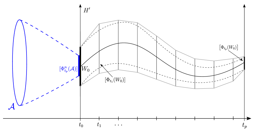
Figure 1: Diagram presenting steps of Algorithm for the proof of Theorem 1.2

8.1 Main algorithm

Input

• $M\geq m>0$, integers, $m$ – the Galerkin projection (12) dimension, and $M$ – the dimension of the finite tail part of self-consistent bounds,

• $[\nu_{1},\nu_{2}]>0$, an interval of the viscosity constant values – can be degenerate (single valued),

• $s\geq 4$, the order of polynomial decay of coefficients that is required from the constructed bounds and trapping regions,

• order and the time step of the Taylor method used by the $C^{0}$ Lohner nonautonomous integrator,

• $t_{p}>0$ period of the nonautonomous forcing,

• the forcing $F$ modes, the autonomous part is provided by $[f_{k}]:=f_{k}+[f_{\varepsilon}]$, where $[f_{\varepsilon}]$ is a uniform and constant perturbation $[f_{\varepsilon}]=[-\varepsilon,\varepsilon]\times[-\varepsilon,\varepsilon]$, and the nonautonomous part is provided by finite number of nonautonomous sufficiently regular $t_{p}$-periodic in time forcing modes $\{\widetilde{f}_{k}(t)\}_{0<|k|\leq m}$, given explicitly in a closed, representable on computer form, allowing automatic differentiation,

• the constants $c_{1}>0$, $c_{2}>0$, and $c_{3}>0$, which should be adjusted according to the equation considered (in our program we have $c_{1}=10^{-5}$, $c_{2}=0.1$, $c_{3}=1.01$).

Output

• $[W]\subset[0,t_{p}]\times H^{\prime}$ – interval representation of $W\subset\mathbb{R}\times H^{\prime}$ – the trapping isolating segment for the discrete semi-process, by representation of a trapping isolating segment we mean interval bounds enclosing $W$, and enclosing all trajectories traversing the trapping isolating segment, this set when glued together bound $W$, $[W]$ is used to calculate the Lipschitz constant bounds,

• $\mathcal{A}\subset H^{\prime}$, an absorbing set forming self-consistent bounds for (6),

• a upper bound for the Lipschitz constant $L=e^{l}$ of $\Phi_{t_{p}}$ on the set $W_{0}$,

begin

1. Using the algorithm from Section 8.2 calculate a set $W_{0}\subset H^{\prime}$ in which $\Phi_{t_{p}}$ is contraction. Verify that $L=e^{l}$ the calculated bound for the Lipschitz constant of $\Phi_{t_{p}}$ on $W_{0}$ satisfies the inequality $L<1$, and therefore there is an (locally) attracting periodic solution within the trapping isolating segment $W$.

2. Using the procedure from [C, Section 8] calculate the absorbing set $\mathcal{A}\subset H^{\prime}$ proved to exist in Thm. 2.9, taking care of the nonautonomous part of forcing. Put

   $$E_{0}=\sup_{\begin{subarray}{c}g\in\left\{[f_{k}]\right\}\\ t\in\mathbb{R}\end{subarray}}{\frac{E(\{g_{k}+\widetilde{f}_{k}(t)\})}{\nu^{2}}},$$ (91)

   and wherever value of $\left|[f_{k}]\right|$ is required, put $\left|[f_{k}]+\sup_{t\in\mathbb{R}}{\widetilde{f}_{k}(t)}\right|$.

3. Using the $C^{0}$ Lohner nonautonomous integrator calculate
   $[\Phi_{t_{p}}^{n}(\mathcal{A})]$ until $n>0$ is found such that $[\Phi_{t_{p}}^{n}(\mathcal{A})]\subset W_{0}$.

end

According to Theorem 2.9 procedure from [C, Section 8] can be modified – value of $\alpha$ (10) can be omitted in the estimates, but then according to Lemma 2.10 there is a penalty – the estimates for the norm are received (compare (19)) instead of estimates for the infimum and supremum.

For cases with $\alpha$ small, the original procedure from [C, Section 8] is expected to be more efficient. Whereas, for cases with $\alpha$ large the estimates based on Lemma 2.10 are expected to be more efficient. The recommended strategy is to calculate estimates using both of the above presented methods, and then take the intersection.

Steps of the algorithm described above are graphically presented on Figure 1.

8.2 Algorithm constructing bounds for trapping isolating segment and estimating Lipschitz constant for time shifts

Input

The same as in the Algorithm from Section 8.1.

Output

• $[W]\subset[0,t_{p}]\times H^{\prime}$ – interval representation of a trapping isolating segment for the discrete semi-process,

• $L>0$ a bound for the Lipschitz constant of $\Phi_{t_{p}}$ on $W_{0}$,

begin

1. Find $\overline{x}$ an approximate location of the fixed point of $\Phi_{t_{p}}$ by applying the Newton method to the map $P_{m}\Phi_{t_{p}}(x)-x$, i.e.

   $$x^{(k+1)}=x^{(k)}-(DP_{m}\Phi_{t_{p}}\left(x^{(k)}\right)-Id)^{-1}\left(P_{m}\Phi_{t_{p}}\left(x^{(k)}\right)-x^{(k)}\right),$$

   stop after several iterations.
   

2. Iteratively find a set $W_{0}\subset H^{\prime}$, such that $\left[\Phi_{t_{p}}(W_{0})\right]\subset~{}W_{0}$ using the following procedure.

   As the initial value of $W_{0}$ take an interval hull of $\overline{x}$ in $H^{\prime}$. Initialize $W_{0}$ by adding $[-c_{1},c_{1}]\times[-c_{1},c_{1}]$ to all coordinates of $\overline{x}$, initialize the tail part $T:=T_{W_{0}}$ with values such that $T_{i}$ satisfy $|T_{i}|\leq C/|i|^{s}$, where $C:=|\left(W_{0}\right)_{m}|\cdot m^{s}$ for $i>m$, and $s$ is provided as an input, $\left(W_{0}\right)_{m}$ denotes the $m$-th coordinate of $W_{0}$.

   while $\left[\Phi_{t_{p}}(W_{0})\right]\nsubseteq W_{0}$ do

   for each $i\in\{1,\dots,M\}$ such that $\left[\Phi_{t_{p}}(W_{0})\right]_{i}\nsubseteq(W_{0})_{i}$ do
   

   if $\left[\Phi_{t_{p}}(W_{0})\right]_{i}^{-}\leq(W_{0})_{i}^{-}$ then
   

   $(W_{0})_{i}^{-}:=\left[\Phi_{t_{p}}(W_{0})\right]_{i}^{-}+c_{2}\cdot\left(\left[\Phi_{t_{p}}(W_{0})\right]_{i}^{-}-(W_{0})_{i}^{-}\right)$
   inflate$\left((W_{0})_{i},c_{3}\right)$
   

   end
   if $\left[\Phi_{t_{p}}(W_{0})\right]_{i}^{+}\geq(W_{0})_{i}^{+}$ then
   

   $(W_{0})_{i}^{+}:=\left[\Phi_{t_{p}}(W_{0})\right]_{i}^{+}+c_{2}\cdot\left(\left[\Phi_{t_{p}}(W_{0})\right]_{i}^{+}-(W_{0})_{i}^{+}\right)$
   inflate$\left((W_{0})_{i},c_{3}\right)$
   

   end
   

   end
   if $C_{T}\cdot(M+1)^{-s_{T}}\leq C_{T_{\Phi_{t_{p}}}}\cdot(M+1)^{-s_{T_{\Phi_{t_{p}}}}}$ then
   

   $C_{T}:=C_{T_{\Phi_{t_{p}}}}\cdot(M+1)^{s_{T}-s_{T_{\Phi_{t_{p}}}}}$
   

   end

   end.
   

3. Using the $C^{0}$ Lohner nonautonomous integrator rigorously integrate $W_{0}$ to obtain bounds along the orbit for the times $t_{1}<\dots<t_{n}<t_{n+1}=t_{p}$, which we denote by $\left[x_{i}\right]$ for $i=1,\dots,n+1$, and $\left[x_{0}\right]:=W_{0}$.

   As the output of our Lohner type algorithm for dPDEs the so-called rough enclosure – rigorous bounds for the solution during the whole time step are obtained, we denote the obtained rough-enclosures by $\left[\varphi\left(t_{i},[0,t_{i+1}-t_{i}],[x_{i}]\right)\right]$ for $i=0,\dots,n$. For $i=0,\dots,n$ the set $\left[\varphi\left(t_{i},[0,t_{i+1}-t_{i}],[x_{i}]\right)\right]$ forms self-consistent bounds for $G$ on $[t_{i},t_{i+1}]$, i.e. satisfy conditions C1, C2, C3 from Definition 6.3.

   In order to calculate the Lipschitz constant of $\Phi_{t_{p}}$ on $W_{0}$ we construct the following interval bounds enclosing the trapping isolating segment for the discrete semi-process, and enclosing all trajectories traversing the trapping isolating segment.

   $$[W]:=\bigcup_{i=0}^{n}[t_{i},t_{i+1}]\times\left[\varphi\left(t_{i},[0,t_{i+1}-t_{i}],[x_{i}]\right)\right].$$

   Then the logarithmic norms are calculated locally on each part of $[W]$.

4. Using the bounds calculated in the previous step calculate local logarithmic norms in a suitable norm. First, calculate an orthogonal change of coordinates $Q_{0}$ such that

   $$[Q_{0}^{-1}]\cdot\frac{\partial P_{m}G}{\partial a}\left(\cdot,\left[\varphi\left(0,[0,t_{1}],W_{0}\right)\right]\right)\cdot Q_{0}$$ (92)

   is in the close to the block-diagonal form. In the equation (92) $Q_{0}$ denotes a point matrix composed of approximate eigenvectors, possibly obtained from a non-rigorous external numerical package, $[Q_{0}^{-1}]$ is the rigorous (interval) inverse of $Q_{0}$, we put $\cdot$ as the first argument of $\frac{\partial P_{m}G}{\partial a}$, because this value is irrelevant (our assumption that the nonautonomous term does not depend on $a$ at all).
   

   for each $i\in\left\{0,\dots,n\right\}$ do
   

   $$\quad\text{calculate }l_{i}:=\mu_{b,\infty}\left(\frac{\partial G}{\partial a}\left(\cdot,\left[\varphi\left(t_{i},[0,t_{i+1}-t_{i}],\left[x_{i}\right]\right)\right]\right)\right)$$ (93)

   end,
   where $\mu_{b,\infty}$ is the logarithmic norm inducted by the block infinity norm defined using the orthogonal change of coordinates $Q_{0}$ (that norm is denoted in Lemma 4.2 by $||\cdot||_{0}$). Obviously $||\cdot||_{0}$ is a compatible norm according to Definition 6.10.

   Observe that at a step $j\colon 0<j\leq n$ in the integration process the matrix $Q_{0}$ can be replaced with another matrix , such that the matrix

   $$[Q_{j}^{-1}]\cdot\frac{\partial P_{m}G}{\partial a}\left(\cdot,\left[\varphi\left(t_{j},[0,t_{j+1}-t_{j}],W_{0}\right)\right]\right)\cdot Q_{j}$$ (94)

   is in the close to a block-diagonal form. Observe that in this case $||\cdot||_{0}=\dots=||\cdot||_{j-1}$, and the local logarithmic norms $l_{j-1}$ and $l_{j}$ are calculated using two distinct norms – $||\cdot||_{0}$ and $||\cdot||_{j}$ respectively.

5. Calculate the global Lipschitz constant using the local logarithmic norms calculated in the previous step. Depending on the number of distinct norms that were used to calculate the local logarithmic norms, two cases are distinguished.

   Case I – only the norm $||\cdot||_{0}$ was used to calculate all of the logarithmic norms $\{l_{i}\}_{i=0}^{n}$ in the previous step. According to Theorem 6.16 the Lipschitz constant of $\Phi_{t_{p}}$ is bounded by $L=Ce^{\frac{l}{\Delta}\Delta}=Ce^{l}$, where $\Delta=t_{p}$, $l=\sum_{i=0}^{n}{l_{i}\cdot(t_{i+1}-t_{i})}$, and $C\geq 1$.
   

   Case II – at least two norms were used to calculate the logarithmic norms $\{l_{i}\}_{i=0}^{n}$ in the previous step of the algorithm. According to Theorem 6.16 the Lipschitz constant of $\Phi_{t_{p}}$ is bounded by $L=Ce^{\frac{l}{\Delta}\Delta}=Ce^{l}$, where $\Delta=t_{p}$, $l=\sum_{i=0}^{n}{l_{i}\cdot(t_{i+1}-t_{i})P_{i\mapsto i+1}}$, and $C\geq 1$.
   

   If the norms $||\cdot||_{j}$ and $||\cdot||_{j+1}$ are different put $P_{j\mapsto j+1}:=||Q_{j+1}^{-1}Q_{j}||_{\infty}$, otherwise, put $P_{j\mapsto j+1}:=1$.
   

   If $l<0$ then the existence of a locally attracting orbit within the set $W$ is claimed.

end

Remark 8.2.

All the bounds for the logarithmic norm of the (infinite dimensional) derivative of vector field $DG$ calculated in the main algorithm presented above are carried out in suitable block coordinates. The finite part of $DP_{m}G$ is reduced by an orthogonal change of coordinates to an (almost) block-diagonal form, i.e. having $2\times 2$ blocks on the diagonal. The block decomposition of $H$ is given by $H=\oplus_{(i)}H_{(i)}$. For $(i)\leq m$ each block $H_{(i)}$ is a two-dimensional eigenspace of $J$. In case of two dimensional blocks $(i)=(i_{1},i_{2})\in\mathbb{Z}^{2}$, the expression $(i)<m$ means that $i_{j}<m$ for $j=1,2$. We consider all blocks two dimensional, and for $(i)>m$ (the infinite dimensional part) the diagonal blocks look like $\left[\begin{array}[]{cc}\lambda_{i}&\alpha_{i}\\ -\alpha_{i}&\lambda_{i}\end{array}\right]$. The logarithmic norm inducted by the euclidean norm of this matrix, is calculated easily, and equals to $\lambda_{i}$. We present explicit estimates that were used in actual computations in [Supplement].

9 Example theorems proved by using presented method

In Table 1 and Table 2 we present data of several theorems that we managed to prove by using the presented method.

To obtain the results presented in Table 1 and Table 2 we kept the forcing constant (it was the same as in Theorem 1.2), and we were varying the parameter $\nu$. The radius of the energy absorbing ball $E_{0}$ (91) was different for each case.

$$\begin{array}[]{|c|c|c|c|c|c|c|c|c|c|c|c|}\hline\cr\mathbf{id}&\mathbf{\nu}&\mathbf{\int_{0}^{2\pi}{u_{0}(x)\,dx}}&\mathbf{E_{0}}&\mathbf{m}&\mathbf{L^{+}}&\textbf{1.}&\textbf{2.}&\textbf{3.}&\textbf{4.}\\ \hline\cr\hline\cr 1(\text{Thm.~{}\ref{thm:main2}})&2&\pi&1.22018&8&3.61879e-05&342.34&\checkmark&\checkmark&\checkmark\\ \hline\cr 2&1.9&0.6\pi&1.352&8&7.38339e-05&365.9&\checkmark&\checkmark&\checkmark\\ \hline\cr 3&1.85&0&1.42607&8&4.64234e-05&933.55&\checkmark&\checkmark&\checkmark\\ \hline\cr 4&1&0&4.88072&14&0.0243972&-^{1}&\checkmark&\checkmark&\\ \hline\cr 5&0.97&0&5.08197&16&0.969176&-^{1}&\checkmark&\checkmark&\\ \hline\cr 6&0.85&0&6.75532&12&3.72357e+24&-^{1}&\checkmark&&\\ \hline\cr\end{array}$$

Table 1: Example results obtained

¹ - we do not provide the total execution time, as we could not perform numerical integration in time in those cases.

$$\begin{array}[]{|c|c|c|c|c|c|c|c|c|c|c|}\hline\cr\mathbf{id}&\mathbf{\nu}&\mathbf{\int_{0}^{2\pi}{u_{0}(x)\,dx}}&\mathbf{E_{0}}&\mathbf{m}&\mathbf{L^{+}}&\textbf{1.}&\textbf{2.}&\textbf{3.}&\textbf{4.}\\ \hline\cr\hline\cr 1&8&200\pi&0.0762613&6&1.59482e-22&806.79&\checkmark&\checkmark&\checkmark\\ \hline\cr 2&0.85&40\pi&6.75532&12&0.00709885&-^{1}&\checkmark&\checkmark&\\ \hline\cr\end{array}$$

Table 2: Example results obtained with large $\alpha=\int_{0}^{2\pi}u_{0}(x)\,dx$

¹ - we do not provide the total execution time, as we could not perform numerical integration in time in those cases.

The meaning of the labels in Table 1 and Table 2 is as follows, 1. is the total execution time in seconds, 2. if the existence of a trapping isolating segment was established, 3. if the periodic solution is locally attracting, 4. if the periodic solution is attracting globally, $L^{+}$ is the upper bound for the Lipschitz constant of $\Phi_{t_{p}}$ – the time shift by $t_{p}$. The order of the Taylor method was $6$, time step length was $0.005$ in all cases.

In some cases, namely in the proofs denoted id 4, 5 in Table 1, and id 2 in Table 2 the numerical integration forward in time of the absorbing set was not performed, as the calculated absorbing set was too large, all attempts to integrate it using our algorithm resulted in blow ups of interval enclosures after a short time. Therefore the step 3 of Algorithm from Section 8.1 was not verified, still, it should be possible also in those cases to perform successfully the step 3 of Algorithm from Section 8.1 by, for instance, applying to the absorbing set some interval set splitting techniques, and then integrate separately each small piece. In the proof denoted id 6 in Table 1 the obtained upper bound for the Lipschitz constant was $>1$, thus we established just the existence of an orbit within the trapping isolating segment, without resolving the question whether this orbit is attracting.

10 Conclusion

A method of proving the existence of globally attracting periodic solutions for a class of dissipative PDEs has been presented. A detailed case study of the viscous Burgers equation with a nonautonomous forcing function has been provided. All the rigorous numerics computer software used is available on-line [Software].

There are several paths for the future development of the presented method we will pursue. First, we will investigate the possibility of obtaining a theoretical result of existence of attracting orbits, with exponential rate of convergence, for (1) with periodic boundary conditions for any forcing, which is a continuous and bounded function of time. We will address this topic in our forthcoming papers.

We would like to conclude with brief note about our forthcoming results [CZ]. We established existence of globally attracting solutions asymptotically for large $\alpha$ ($u_{0}$ integral). Additionally, in this case, we obtained bounds for the attracting solution of the form $\alpha+O(\frac{\|f\|}{\alpha})$. In this work we also considered the whole class of smooth forcings, i.e. we dropped the assumption of the finite number of nonzero forcing modes.

Appendix A Numerical data from proof of Theorem 1.2

In this appendix we present the numerical data obtained in the algorithm from Section 8.1 proving Theorem 1.2.

Program was programmed in C++ language. Program was executed on Linux 32-bit Intel Core i5-2430M CPU @ 2.40 GHz x 4 machine, compiled with GCC compiler version 4.7.3, and with the following compiler flags (-O0 -frounding-math -ffloat-store).

• The Galerkin projection dimension, $m=8$.

• The autonomous forcing $l^{2}$ energy, $E(\{f_{k}\})=1.31$.

• The nonautonomous forcing $l^{2}$ energy, $E(\{\widetilde{f}_{k}\})=1.31$.

• Upper bound for the total forcing $l^{2}$ energy,

  $$\max_{\begin{subarray}{c}g\in\left\{[f_{k}]\right\}\\ t\in[0,t_{p}]\end{subarray}}{E(\{g_{k}+\widetilde{f}_{k}(t)\})}=4.88072.$$

• The absorbing ball radius $E_{0}=1.22018$.

• The Lipschitz constant, $L\leq 3.61879e-05$.

• The absorbing set, $V\oplus\Theta=$

  $$\begin{array}[]{|c|c|c|}\hline\cr\mathbf{k}&\mathbf{\operatorname{Re}\left(a_{k}\right)}&\mathbf{\operatorname{Im}\left(a_{k}\right)}\\ \hline\cr\hline\cr 1&0.0259487+[-0.357457,0.357457]&0.153052+[-0.238867,0.238867]\\ 2&0.0449597+[-0.150289,0.150289]&-0.0425997+[-0.143525,0.143525]\\ 3&-0.0178005+[-7.0412,7.0412]10^{-2}&0.0192868+[-7.07427,7.07427]10^{-2}\\ 4&-1.75301\cdot 10^{-3}+[-2.24348,2.24348]10^{-2}&1.45325\cdot 10^{-3}+[-2.23378,2.23378]10^{-2}\\ 5&8.24378\cdot 10^{-4}+[-9.60379,9.60379]10^{-3}&1.45682\cdot 10^{-4}+[-9.60024,9.60024]10^{-3}\\ 6&-3.07739\cdot 10^{-5}+[-4.3149,4.3149]10^{-3}&-1.0924\cdot 10^{-5}+[-4.30936,4.30936]10^{-3}\\ 7&-4.5983\cdot 10^{-5}+[-2.01048,2.01048]10^{-3}&-1.49242\cdot 10^{-5}+[-2.01036,2.01036]10^{-3}\\ 8&-1.96036\cdot 10^{-6}+[-9.87006,9.87006]10^{-4}&7.01463\cdot 10^{-6}+[-9.86863,9.86863]10^{-4}\\ 9&2.81191\cdot 10^{-6}+[-6.19244,6.19244]10^{-4}&4.15566\cdot 10^{-6}+[-6.19241,6.19241]10^{-4}\\ 10&-2.16324\cdot 10^{-7}+[-4.00182,4.00182]10^{-4}&-1.24755\cdot 10^{-6}+[-3.99861,3.99861]10^{-4}\\ 11&-1.10967\cdot 10^{-7}+[-2.84633,2.84633]10^{-4}&-1.0639\cdot 10^{-7}+[-2.84634,2.84634]10^{-4}\\ 12&-5.47851\cdot 10^{-8}+[-2.18552,2.18552]10^{-4}&1.37878\cdot 10^{-7}+[-2.18508,2.18508]10^{-4}\\ 13&1.29273\cdot 10^{-8}+[-1.77235,1.77235]10^{-4}&-1.69395\cdot 10^{-8}+[-1.77237,1.77237]10^{-4}\\ 14&9.27549\cdot 10^{-9}+[-1.49524,1.49524]10^{-4}&-1.9964\cdot 10^{-9}+[-1.4952,1.4952]10^{-4}\\ 15&-4.70792\cdot 10^{-9}+[-1.29781,1.29781]10^{-4}&-2.81077\cdot 10^{-10}+[-1.29781,1.29781]10^{-4}\\ 16&4.35414\cdot 10^{-10}+[-1.15017,1.15017]10^{-4}&-2.87508\cdot 10^{-10}+[-1.15016,1.15016]10^{-4}\\ 17&4.76886\cdot 10^{-10}+[-1.03539,1.03539]10^{-4}&2.82898\cdot 10^{-10}+[-1.03539,1.03539]10^{-4}\\ 18&-2.05696\cdot 10^{-10}+[-9.43268,9.43268]10^{-5}&-8.29394\cdot 10^{-11}+[-9.43267,9.43267]10^{-5}\\ 19&-4.29042\cdot 10^{-12}+[-8.67209,8.67209]10^{-5}&-1.99325\cdot 10^{-11}+[-8.67208,8.67208]10^{-5}\\ 20&1.68368\cdot 10^{-11}+[-8.02637,8.02637]10^{-5}&2.14338\cdot 10^{-11}+[-8.02637,8.02637]10^{-5}\\ 21&-1.01567\cdot 10^{-11}+[-7.46033,7.46033]10^{-5}&-1.19795\cdot 10^{-11}+[-7.46033,7.46033]10^{-5}\\ 22&1.67491\cdot 10^{-12}+[-6.93165,6.93165]10^{-5}&4.91813\cdot 10^{-12}+[-6.93165,6.93165]10^{-5}\\ 23&2.14631\cdot 10^{-13}+[-6.41116,6.41116]10^{-5}&-1.35591\cdot 10^{-12}+[-6.41116,6.41116]10^{-5}\\ \geq 24&\vrule\lx@intercol\hfil|a_{k}|\leq 11362.2/k^{5},\ |a_{24}|=-2.41124\cdot 10^{-14}+[-5.86026,5.86026]10^{-5}\hfil\lx@intercol\vrule\lx@intercol\\ \hline\cr\end{array}$$

• The trapping region, $W=$

  $$\begin{array}[]{|c|c|c|}\hline\cr\mathbf{k}&\mathbf{\operatorname{Re}\left(a_{k}\right)}&\mathbf{\operatorname{Im}\left(a_{k}\right)}\\ \hline\cr\hline\cr 1&0.0862439+[-1,1]10^{-4}&0.11949+[-1,1]10^{-4}\\ 2&0.0376504+[-1,1]10^{-4}&-0.0422059+[-1,1]10^{-4}\\ 3&-0.0192285+[-1,1]10^{-4}&0.021161+[-1,1]10^{-4}\\ 4&-2.03091\cdot 10^{-4}+[-1,1]10^{-4}&5.43697\cdot 10^{-4}+[-1,1]10^{-4}\\ 5&1.56511\cdot 10^{-4}+[-1,1]10^{-4}&-1.51924\cdot 10^{-5}+[-1,1]10^{-4}\\ 6&-2.91075\cdot 10^{-5}+[-1,1]10^{-4}&1.7875\cdot 10^{-6}+[-1,1]10^{-4}\\ 7&-1.7401\cdot 10^{-6}+[-1,1]10^{-4}&4.24224\cdot 10^{-7}+[-1,1]10^{-4}\\ 8&2.88967\cdot 10^{-7}+[-1,1]10^{-4}&2.38365\cdot 10^{-7}+[-1,1]10^{-4}\\ 9&0+[-6.24295,6.24295]10^{-5}&0+[-6.24295,6.24295]10^{-5}\\ 10&0+[-4.096,4.096]10^{-5}&0+[-4.096,4.096]10^{-5}\\ 11&0+[-2.79762,2.79762]10^{-5}&0+[-2.79762,2.79762]10^{-5}\\ 12&0+[-1.97531,1.97531]10^{-5}&0+[-1.97531,1.97531]10^{-5}\\ 13&0+[-1.43412,1.43412]10^{-5}&0+[-1.43412,1.43412]10^{-5}\\ 14&0+[-1.06622,1.06622]10^{-5}&0+[-1.06622,1.06622]10^{-5}\\ 15&0+[-8.09086,8.09086]10^{-6}&0+[-8.09086,8.09086]10^{-6}\\ 16&0+[-6.25,6.25]10^{-6}&0+[-6.25,6.25]10^{-6}\\ 17&0+[-4.90416,4.90416]10^{-6}&0+[-4.90416,4.90416]10^{-6}\\ 18&0+[-3.90184,3.90184]10^{-6}&0+[-3.90184,3.90184]10^{-6}\\ 19&0+[-3.14301,3.14301]10^{-6}&0+[-3.14301,3.14301]10^{-6}\\ 20&0+[-2.56,2.56]10^{-6}&0+[-2.56,2.56]10^{-6}\\ 21&0+[-2.10612,2.10612]10^{-6}&0+[-2.10612,2.10612]10^{-6}\\ 22&0+[-1.74851,1.74851]10^{-6}&0+[-1.74851,1.74851]10^{-6}\\ 23&0+[-1.46369,1.46369]10^{-6}&0+[-1.46369,1.46369]10^{-6}\\ \geq 24&\vrule\lx@intercol\hfil|a_{k}|\leq 0.4096/k^{4},\ |a_{24}|=0+[-1.23457,1.23457]10^{-6}\hfil\lx@intercol\vrule\lx@intercol\\ \hline\cr\end{array}$$

• Approximate eigenvalues of $D\,P_{m}G\left(\operatorname{mid}\left(\left[\varphi\left([t_{0},t_{1}],0,W\right)\right]\right)\right)$ matrix (92), $\operatorname{spect}\left(D\,P_{m}G\left(\operatorname{mid}\left(\left[\varphi\left([t_{0},t_{1}],0,W\right)\right]\right)\right)\right)=$

  $$\left\{-127.956+i4.00124,-127.956-i4.00124,-98.0028+i3.49945,-98.0028-i3.49945,\right.$$

  $$-2.00765+i0.496188,-2.00765-i0.496188,-8.00731+i0.999835,-8.00731-i0.999835,$$

  $$-18.0068+i1.49997,-18.0068-i1.49997,-32.0066+i1.99999,-32.0066-i1.99999,$$

  $$\left.-72.006+i2.99993,-72.006-i2.99993,-50.0065+i2.49999,-50.0065-i2.49999\right\}.$$ (95)

The absorbing set is apparently larger than the trapping region, it was necessary for the proof to integrate it rigorously forward in time. The Taylor method used in the $C^{0}$ Lohner nonautonomous integrator was of order $6$ with time step $0.005$. Total execution time was $342.34$ seconds.

Here we presented data limited to 6, more detailed numerical data with higher precision is available on-line at [Software].

References

• [Software] Software used in this paper, http://ww2.ii.uj.edu.pl/~cyranka/NonautonomousBurgers/ (alt. link www.cyranka.net).
• [Supplement] Supplementary material, http://ww2.ii.uj.edu.pl/~cyranka/NonautonomousBurgers/ (alt. link www.cyranka.net).
• [B] J.M. Burgers, A mathematical model illustrating the theory of turbulence, Adv. Appl. Mech., vol 1(1948), 171-199.
• [CAPD] CAPD - Computer Assisted Proofs in Dynamics, a package for rigorous numeric, http://capd.ii.uj.edu.pl.
• [C] J. Cyranka, Existence of globally attracting fixed points of viscous Burgers equation with constant forcing. A computer assisted proof. TMNA, accepted.
• [C2] J. Cyranka, Efficient Algorithms for Rigorous Integration Forward in Time of dPDEs. Existence of Globally Attracting Fixed Points of Viscous Burgers Equation with Constant Forcing, a Computer Assisted Proof, PhD dissertation, Jagiellonian University, Kraków, 2013, available on-line http://ww2.ii.uj.edu.pl/~cyranka (alt. link www.cyranka.net).
• [CZ] J. Cyranka, P. Zgliczyński, The effect of fast movement in dissipative PDEs with the forcing term, arXiv:1407.1712 [math.DS].
• [D] G. Dahlquist, Stability and Error Bounds in the Numerical Intgration of Ordinary Differential Equations, Almqvist & Wiksells, Uppsala, 1958; Transactions of the Royal Institute of Technology, Stockholm, 1959.
• [FMRT] C. Foias, O. Manley, R. Rosa, R. Temam Navier-Stokes Equations and Turbulence, Encyclopedia of Mathematics and Its Applications, Vol. 84, Cambridge Univeristy Press, 2008.
• [HNW] E. Hairer, S.P. Nørsett and G. Wanner, Solving Ordinary Differential Equations I, Nonstiff Problems, Springer-Verlag, Berlin Heidelberg 1987.
• [JKM] H.R. Jauslin, H.O. Kreiss, J. Moser, On the Forced Burgers Equation with Periodic Boundary Condition, Proceedings of Symposia in Pure Mathematics, Vol. 65, 1999.
• [KZ] T. Kapela and P. Zgliczyński, A Lohner-type algorithm for control systems and ordinary differential inclusions, Discrete Cont. Dyn. Sys. B, vol. 11(2009), 365-385.
• [Lo1] R.J. Lohner, Einschliessung der Lösung gewöhnlicher Anfangs und Randwertaufgaben und Anwendungen, Universität Karlsruhe (TH), these 1988.
• [Lo] R.J. Lohner, Computation of Guaranteed Enclosures for the Solutions of Ordinary Initial and Boundary Value Problems, Computational Ordinary Differential Equations, J.R. Cash, I. Gladwell Eds., Clarendon Press, Oxford, 1992.
• [L] S. M. Lozinskii, Error esitimates for the numerical integration of ordinary differential equations, part I, Izv. Vyss. Uceb. Zaved. Matematica,6 (1958), 52–90 (Russian)
• [Si1] Ya. Sinai, Two Results Concerning Asymptotic Behavior of Solutions of Burgers Equation with Force, Journal of Statistical Physics, 64 (1991), 1–12.
• [S1] R. Srzednicki, Periodic and bounded solutions in blocks for time-periodic nonautonomuous ordinary differential equations. Nonlin. Analysis, TMA., 1994, 22, 707–737.
• [SW] R. Srzednicki & K. Wójcik, A geometric method for detecting chaotic dynamics, J. Diff. Eq., 1997, 135, 66–82.
• [W] W. Walter, Differential and integral inequalities, Springer-Verlag Berlin Heidelberg New York, 1970.
• [Wh] G. B. Whitham, Linear and Nonlinear Waves. John Wiley & Sons, 1975.
• [ZM] P. Zgliczyński and K. Mischaikow, Rigorous Numerics for Partial Differential Equations: the Kuramoto-Sivashinsky equation, Foundations of Computational Mathematics, vol. 1(2001), 255-288.
• [ZAKS] P. Zgliczyński, Attracting fixed points for the Kuramoto-Sivashinsky equation - a computer assisted proof, SIAM Journal on Applied Dynamical Systems, vol. 1(2002), 215-288.
• [ZNS] P. Zgliczyński, Trapping regions and an ODE-type proof of an existence and uniqueness for Navier-Stokes equations with periodic boundary conditions on the plane, Univ. Iag. Acta Math., vol. 41(2003), 89-113.
• [Z2] P. Zgliczyński, Rigorous numerics for dissipative Partial Differential Equations II. Periodic orbit for the Kuramoto-Sivashinsky PDE - a computer assisted proof, Foundations of Computational Mathematics, vol. 4(2004), 157-185.
• [Z3] P. Zgliczyński, Rigorous Numerics for Dissipative PDEs III. An effective algorithm for rigorous integration of dissipative PDEs, Topological Methods in Nonlinear Analysis, vol. 36(2010), 197-262.