Tight Bounds for Symmetric Divergence Measures and a Refined Bound for Lossless Source Coding

Abstract

Tight bounds for several symmetric divergence measures are derived in terms of the total variation distance. It is shown that each of these bounds is attained by a pair of 2 or 3-element probability distributions. An application of these bounds for lossless source coding is provided, refining and improving a certain bound by Csiszár. Another application of these bounds has been recently introduced by Yardi. et al. for channel-code detection.

Index Terms – Bhattacharyya distance, Chernoff information, $f$-divergence, Jeffreys’ divergence, lossless source coding, total variation distance.

I Introduction

Divergence measures are widely used in information theory, machine learning, statistics, and other theoretical and applied branches of mathematics (see, e.g., [2], [9], [10], [23]). The class of $f$-divergences, introduced independently in [1, 6] and [22], forms an important class of divergence measures. Their properties, including relations to statistical tests and estimators, were studied, e.g., in [9] and [20].

In [14], Gilardoni studied the problem of minimizing an arbitrary symmetric $f$-divergence for a given total variation distance, providing a closed-form solution of this optimization problem. In a follow-up paper by the same author [15], Pinsker’s and Vajda’s type inequalities were studied for symmetric $f$-divergences, and the issue of obtaining lower bounds on $f$-divergences for a fixed total variation distance was further studied. One of the main results in [15] was a derivation of a simple closed-form lower bound on the relative entropy in terms of the total variation distance, which suggests an improvement over Pinsker’s and Vajda’s inequalities, and a derivation of a simple and reasonably tight closed-form upper bound on the infimum of the relative entropy in terms of the total variation distance.

An exact characterization of the minimum of the relative entropy subject to a fixed total variation distance has been derived in [13] and [14]. More generally, sharp inequalities for $f$-divergences were recently studied in [16] as a problem of maximizing or minimizing an arbitrary $f$-divergence between two probability measures subject to a finite number of inequality constraints on other $f$-divergences. The main result stated in [16] is that such infinite-dimensional optimization problems are equivalent to optimization problems over finite-dimensional spaces where the latter are numerically solvable.

Following previous work, tight bounds on symmetric $f$-divergences and related distances are derived in this paper. An application of these bounds for lossless source coding is provided, refining and improving a certain bound by Csiszár from 1967 [7].

The paper is organized as follows: preliminary material is introduced in Section II, tight bounds for several symmetric divergence measures, which are either symmetric $f$-divergences or related symmetric distances, are derived in Section III; these bounds are expressed in terms of the total variation distance, and their tightness is demonstrated. One of these bounds is used in Section IV for the derivation of an improved and refined bound for lossless source coding.

II Preliminaries

We introduce, in the following, some preliminaries and notation that are essential to this paper.

Definition 1

Let $P$ and $Q$ be two probability distributions with a common $\sigma$-algebra $\mathcal{F}$. The total variation distance between $P$ and $Q$ is defined by

$$d_{\text{TV}}(P,Q)\triangleq\sup_{A\in\mathcal{F}}|P(A)-Q(A)|.$$ (1)

If $P$ and $Q$ are defined on a countable set, (1) is simplified to

$$d_{\text{TV}}(P,Q)=\frac{1}{2}\sum_{x}\bigl{|}P(x)-Q(x)\bigr{|}=\frac{||P-Q||_{1}}{2}$$ (2)

so it is equal to one-half the $L_{1}$-distance between $P$ and $Q$.

Definition 2

Let $f\colon(0,\infty)\rightarrow{\rm I\!R}$ be a convex function with $f(1)=0$, and let $P$ and $Q$ be two probability distributions. The $f$-divergence from $P$ to $Q$ is defined by

$$D_{f}(P||Q)\triangleq\sum_{x}Q(x)\,f\left(\frac{P(x)}{Q(x)}\right)$$ (3)

with the convention that

$$\ 0f\Bigl{(}\frac{0}{0}\Bigr{)}=0,\quad f(0)=\lim_{t\rightarrow 0^{+}}f(t),$$

$$\ 0f\Bigl{(}\frac{a}{0}\Bigr{)}=\lim_{t\rightarrow 0^{+}}tf\Bigl{(}\frac{a}{t}\Bigr{)}=a\lim_{u\rightarrow\infty}\frac{f(u)}{u},\quad\forall\,a>0.$$

Definition 3

An $f$-divergence is symmetric if $D_{f}(P||Q)=D_{f}(Q||P)$ for every $P$ and $Q$.

Symmetric $f$-divergences include (among others) the squared Hellinger distance where

$$f(t)=(\sqrt{t}-1)^{2},\quad D_{f}(P||Q)=\sum_{x}\left(\sqrt{P(x)}-\sqrt{Q(x)}\right)^{2},$$

and the total variation distance in (2) where $f(t)=\frac{1}{2}\,|t-1|.$

An $f$-divergence is symmetric if and only if the function $f$ satisfies the equality (see [14, p. 765])

$$f(u)=u\,f\left(\frac{1}{u}\right)+a(u-1),\quad\forall\,u\in(0,\infty)$$ (4)

for some constant $a$. If $f$ is differentiable at $u=1$ then a differentiation of both sides of equality (4) at $u=1$ gives that $a=2f^{\prime}(1)$.

Note that the relative entropy (a.k.a. the Kullback-Leibler divergence) $D(P||Q)\triangleq\sum_{x}P(x)\log\left(\frac{P(x)}{Q(x)}\right)$ is an $f$-divergence with $f(t)=t\log(t),\;t>0$; its dual, $D(Q||P)$, is an f-divergence with $f(t)=-\log(t),\;t>0$; clearly, it is an asymmetric $f$-divergence since $D(P||Q)\neq D(Q||P)$ .

The following result, which was derived by Gilardoni (see [14, 15]), refers to the infimum of a symmetric $f$-divergence for a fixed value of the total variation distance:

Theorem 1

Let $f\colon(0,\infty)\rightarrow{\rm I\!R}$ be a convex function with $f(1)=0$, and assume that $f$ is twice differentiable. Let

$$L_{D_{f}}(\varepsilon)\triangleq\inf_{P,Q\colon\,d_{\text{TV}}(P,Q)=\varepsilon}D_{f}(P||Q),\quad\forall\,\varepsilon\in[0,1]$$ (5)

be the infimum of the $f$-divergence for a given total variation distance. If $D_{f}$ is a symmetric $f$-divergence, and $f$ is differentiable at $u=1$, then

$$L_{D_{f}}(\varepsilon)=(1-\varepsilon)\,f\left(\frac{1+\varepsilon}{1-\varepsilon}\right)-2f^{\prime}(1)\,\varepsilon,\quad\forall\,\varepsilon\in[0,1].$$ (6)

Consider an arbitrary symmetric $f$-divergence. Note that it follows from (4) and (6) that the infimum in (5), is attained by the pair of 2-element probability distributions where

$$P=\left(\frac{1-\varepsilon}{2},\,\frac{1+\varepsilon}{2}\right),\quad Q=\left(\frac{1+\varepsilon}{2},\,\frac{1-\varepsilon}{2}\right)$$

(or by switching $P$ and $Q$ since $D_{f}$ is assumed to be a symmetric divergence).

Throughout this paper, the logarithms are on base $e$ unless the base of the logarithm is stated explicitly.

III Derivation of Tight Bounds on Symmetric Divergence Measures

The following section introduces tight bounds for several symmetric divergence measures for a fixed value of the total variation distance. The statements are introduced in Section III-A–III-D, their proof are provided in (III-E), followed by discussions on the statements in Section III-F.

III-A Tight Bounds on the Bhattacharyya Coefficient

Definition 4

Let $P$ and $Q$ be two probability distributions that are defined on the same set. The Bhattacharyya coefficient [18] between $P$ and $Q$ is given by

$$Z(P,Q)\triangleq\sum_{x}\sqrt{P(x)\,Q(x)}\,.$$ (7)

The Bhttacharyya distance is defined as minus the logarithm of the Bhattacharyya coefficient, so that it is zero if and only if $P=Q$, and it is non-negative in general (since $0\leq Z(P,Q)\leq 1$, and $Z(P,Q)=1$ if and only if $P=Q$).

Proposition 1

Let $P$ and $Q$ be two probability distributions. Then, for a fixed value $\varepsilon\in[0,1]$ of the total variation distance (i.e., if $d_{\text{TV}}(P,Q)=\varepsilon$), the respective Bhattacharyya coefficient satisfies the inequality

$$1-\varepsilon\leq Z(P,Q)\leq\sqrt{1-\varepsilon^{2}}.$$ (8)

Both upper and lower bounds are tight: the upper bound is attained by the pair of 2-element probability distributions

$$P=\left(\frac{1-\varepsilon}{2},\,\frac{1+\varepsilon}{2}\right),\quad Q=\left(\frac{1+\varepsilon}{2},\,\frac{1-\varepsilon}{2}\right),$$

and the lower bound is attained by the pair of 3-element probability distributions

$$P=(\varepsilon,1-\varepsilon,0),\quad Q=(0,1-\varepsilon,\varepsilon).$$

III-B A Tight Bound on the Chernoff Information

Definition 5

The Chernoff information between two probability distributions $P$ and $Q$, defined on the same set, is given by

$$C(P,Q)\triangleq-\min_{\lambda\in[0,1]}\;\log\left(\sum_{x}P(x)^{\lambda}\,Q(x)^{1-\lambda}\right).$$ (9)

Note that

$$C(P,Q) =\max_{\lambda\in[0,1]}\left\{-\log\left(\sum_{x}P(x)^{\lambda}\,Q(x)^{1-\lambda}\right)\right\}$$

$$=\max_{\lambda\in(0,1)}\,\Bigl{\{}(1-\lambda)\,D_{\lambda}(P,Q)\Bigr{\}}$$ (10)

where $D_{\lambda}(P,Q)$ designates the Rényi divergence of order $\lambda$ [12]. The endpoints of the interval $[0,1]$ are excluded in the second line of (10) since the Chernoff information is non-negative, and the logarithmic function in the first line of (10) is equal to zero at both endpoints.

Proposition 2

Let

$$C(\varepsilon)\triangleq\min_{P,Q\colon\,d_{\text{TV}}(P,Q)=\varepsilon}C(P,Q),\quad\forall\,\varepsilon\in[0,1]$$ (11)

be the minimum of the Chernoff information for a fixed value $\varepsilon\in[0,1]$ of the total variation distance. This minimum indeed exists, and it is equal to

$$C(\varepsilon)=\left\{\begin{array}[]{ll}-\frac{1}{2}\,\log(1-\varepsilon^{2})&\mbox{if $\varepsilon\in[0,1)$}\\[2.84544pt] +\infty&\mbox{if $\varepsilon=1$.}\end{array}\right.$$ (12)

For $\varepsilon\in[0,1)$, it is achieved by the pair of 2-element probability distributions $P=\left(\frac{1-\varepsilon}{2},\,\frac{1+\varepsilon}{2}\right)$, and $Q=\left(\frac{1+\varepsilon}{2},\,\frac{1-\varepsilon}{2}\right)$.

Corollary 1

For any pair of probability distributions $P$ and $Q$,

$$C(P,Q)\geq-\frac{1}{2}\log\Bigl{(}1-\bigl{(}d_{\text{TV}}(P,Q)\bigr{)}^{2}\Bigr{)}.$$ (13)

and this lower bound is tight for a given value of the total variation distance.

Remark 1 (An Application of Corollary 1)

From Corollary 1, a lower bound on the total variation distance implies a lower bound on the Chernoff information; consequently, it provides an upper bound on the best achievable Bayesian probability of error for binary hypothesis testing (see, e.g., [5, Theorem 11.9.1]). This approach has been recently used in [26] to obtain a lower bound on the Chernoff information for studying a communication problem that is related to channel-code detection via the likelihood ratio test (the authors in [26] refer to our previously un-published manuscript [24], where this corollary first appeared).

III-C A Tight Bound on the Capacitory Discrimination

The capacitory discrimination (a.k.a. the Jensen-Shannon divergence) is defined as follows:

Definition 6

Let $P$ and $Q$ be two probability distributions. The capacitory discrimination between $P$ and $Q$ is given by

$$\begin{split}\overline{C}(P,Q)&\ \triangleq D\left(P\,||\,\frac{P+Q}{2}\right)+D\left(Q\,||\,\frac{P+Q}{2}\right)\\ &\ =2\left[H\left(\frac{P+Q}{2}\right)-\frac{H(P)+H(Q)}{2}\right]\end{split}$$ (14)

where $H(P)\triangleq-\sum_{x}P(x)\,\log P(x)$.

This divergence measure was studied in [3], [4], [11], [16], [21] and [25]. Due to the parallelogram identity for relative entropy (see, e.g., [8, Problem 3.20]), it follows that $\overline{C}(P,Q)=\min\bigl{\{}D(P||R)+D(Q||R)\bigr{\}}$ where the minimization is taken w.r.t. all probability distributions $R$.

Proposition 3

For a given value $\varepsilon\in[0,1]$ of the total variation distance, the minimum of the capacitory discrimination is equal to

$$\min_{P,Q\colon\,d_{\text{TV}}(P,Q)=\varepsilon}\overline{C}(P,Q)=2\,d\left(\frac{1-\varepsilon}{2}\,\big{|}\big{|}\,\frac{1}{2}\right)$$ (15)

and it is achieved by the 2-element probability distributions $P=\left(\frac{1-\varepsilon}{2},\,\frac{1+\varepsilon}{2}\right)$, and $Q=\left(\frac{1+\varepsilon}{2},\,\frac{1-\varepsilon}{2}\right)$. In (15),

$$d(p||q)\triangleq p\log\left(\frac{p}{q}\right)+(1-p)\log\left(\frac{1-p}{1-q}\right),\quad p,q\in[0,1],$$ (16)

with the convention that $0\log 0=0$, denotes the divergence (relative entropy) between the two Bernoulli distributions with parameters $p$ and $q$.

Remark 2

The lower bound on the capacitory discrimination was obtained independently by Briët and Harremoës (see [3, Eq. (18)] for $\alpha=1$) whose derivation was based on a different approach.

The following result provides a measure of the concavity of the entropy function:

Corollary 2

For arbitrary probability distributions $P$ and $Q$, the following inequality holds:

$$H\left(\frac{P+Q}{2}\right)-\frac{H(P)+H(Q)}{2}\geq d\left(\frac{1-d_{\text{TV}}(P,Q)}{2}\,\big{|}\big{|}\,\frac{1}{2}\right)$$

and this lower bound is tight for a given value of the total variation distance.

III-D Tight Bounds on Jeffreys’ divergence

Definition 7

Let $P$ and $Q$ be two probability distributions. Jeffreys’ divergence [17] is a symmetrized version of the relative entropy, which is defined as

$$J(P,Q)\triangleq\frac{D(P||Q)+D(Q||P)}{2}.$$ (17)

This forms a symmetric $f$-divergence where $J(P,Q)=D_{f}(P||Q)$ with

$$f(t)=\frac{(t-1)\log(t)}{2}\,,\quad t>0,$$ (18)

which is a convex function on $(0,\infty)$, and $f(1)=0$.

Proposition 4

$$\min_{P,Q\colon d_{\text{TV}}(P,Q)=\varepsilon}J(P,Q)=\varepsilon\,\log\left(\frac{1+\varepsilon}{1-\varepsilon}\right),\quad\forall\,\varepsilon\in[0,1),$$ (19)

$$\inf_{P,Q\colon D(P||Q)=\varepsilon}J(P,Q)=\frac{\varepsilon}{2},\quad\forall\,\varepsilon>0,$$ (20)

and the two respective suprema are equal to $+\infty$. The minimum of Jeffreys’ divergence in (19), for a fixed value $\varepsilon$ of the total variation distance, is achieved by the pair of 2-element probability distributions $P=\left(\frac{1-\varepsilon}{2},\,\frac{1+\varepsilon}{2}\right)$ and $Q=\left(\frac{1+\varepsilon}{2},\,\frac{1-\varepsilon}{2}\right)$.

III-E Proofs

III-E1 Proof of Proposition 1

From (2), (7) and the Cauchy-Schwartz inequality, we have

$$d_{\text{TV}}(P,Q) =\frac{1}{2}\,\sum_{x}\left|P(x)-Q(x)\right|$$

$$=\frac{1}{2}\,\sum_{x}\left|\sqrt{P(x)}-\sqrt{Q(x)}\,\right|\left(\sqrt{P(x)}+\sqrt{Q(x)}\,\right)$$

$$\leq\frac{1}{2}\,\left(\sum_{x}\left(\sqrt{P(x)}-\sqrt{Q(x)}\,\right)^{2}\right)^{\frac{1}{2}}\left(\sum_{x}\left(\sqrt{P(x)}+\sqrt{Q(x)}\,\right)^{2}\right)^{\frac{1}{2}}$$

$$=\frac{1}{2}\bigl{(}2-2Z(P,Q)\bigr{)}^{\frac{1}{2}}\bigl{(}2+2Z(P,Q)\bigr{)}^{\frac{1}{2}}$$

$$=\left(1-Z^{2}(P,Q)\right)^{\frac{1}{2}}$$

which implies that $Z(P,Q)\leq\left(1-d_{\text{TV}}^{2}(P,Q)\right)^{\frac{1}{2}}$. This gives the upper bound on the Bhattacharyya coefficient in (8). For proving the lower bound, note that

$$Z(P,Q) =1-\frac{1}{2}\sum_{x}\Bigl{(}\sqrt{P(x)}-\sqrt{Q(x)}\Bigr{)}^{2}$$

$$=1-\frac{1}{2}\sum_{x}|P(x)-Q(x)|\left(\frac{|\sqrt{P(x)}-\sqrt{Q(x)}|}{\sqrt{P(x)}+\sqrt{Q(x)}}\right)$$

$$\geq 1-\frac{1}{2}\sum_{x}|P(x)-Q(x)|=1-d_{\text{TV}}(P,Q).$$

The tightness of the bounds on the Bhattacharyya coefficient in terms of the total variation distance is proved in the following. For a fixed value of the total variation distance $\varepsilon\in[0,1]$, let $P$ and $Q$ be the pair of 2-element probability distributions $P=\left(\frac{1-\varepsilon}{2},\,\frac{1+\varepsilon}{2}\right)$ and $Q=\left(\frac{1+\varepsilon}{2},\,\frac{1-\varepsilon}{2}\right)$. This gives

$$d_{\text{TV}}(P,Q)=\varepsilon,\quad Z(P,Q)=\sqrt{1-\varepsilon^{2}}$$

so the upper bound is tight. Furthermore, for the pair of 3-element probability distributions $P=(\varepsilon,1-\varepsilon,0)$ and $Q=(0,1-\varepsilon,\varepsilon)$, we have

$$d_{\text{TV}}(P,Q)=\varepsilon,\quad Z(P,Q)=1-\varepsilon$$

so also the lower bound is tight.

Remark 3

The lower bound on the Bhattacharyya coefficient in (8) dates back to Kraft [19, Lemma 1], though its proof was simplified here.

Remark 4

Both the Bhattacharyya distance and coefficient are functions of the Hellinger distance, so a tight upper bound on the Bhattacharyya coefficient in terms of the total variation distance can be also obtained from a tight upper bound on the Hellinger distance (see [16, p. 117]).

III-E2 Proof of Proposition 2

$$C(P,Q)\stackrel{{\scriptstyle(\text{a})}}{{\geq}}-\log\left(\sum_{x}\sqrt{P(x)\,Q(x)}\right)$$

$$\hskip 42.67912pt\stackrel{{\scriptstyle(\text{b})}}{{=}}-\log\,Z(P,Q)$$

$$\hskip 42.67912pt\stackrel{{\scriptstyle(\text{c})}}{{\geq}}-\frac{1}{2}\log\Bigl{(}1-\bigl{(}d_{\text{TV}}(P,Q)\bigr{)}^{2}\Bigr{)}$$

where inequality (a) follows by selecting the possibly sub-optimal value of $\lambda=\frac{1}{2}$ in (9), equality (b) holds by definition (see (7)), and inequality (c) follows from the upper bound on the Bhattacharyya distance in (8). By the definition in (11), it follows that

$$C(\varepsilon)\geq-\frac{1}{2}\,\log(1-\varepsilon^{2}).$$ (21)

In order to show that (21) provides a tight lower bound for a fixed value of the total variation distance $(\varepsilon)$, note that for the pair of 2-element probability distributions $P$ and $Q$ in Proposition 2, the Chernoff information in (9) is given by

$$C(P,Q)=-\min_{\lambda\in[0,1]}\log\left(\frac{1-\varepsilon}{2}\left(\frac{1+\varepsilon}{1-\varepsilon}\right)^{\lambda}+\frac{1+\varepsilon}{2}\left(\frac{1-\varepsilon}{1+\varepsilon}\right)^{\lambda}\right).$$ (22)

A minimization of the function in (22) gives that $\lambda=\frac{1}{2}$, and

$$C(P,Q)=-\frac{1}{2}\,\log(1-\varepsilon^{2}),$$

which implies that the lower bound in (21) is tight.

III-E3 Proof of Proposition 3

In [16, p. 119], the capacitory discrimination is expressed as an $f$-divergence where

$$f(x)=x\log x-(x+1)\log(1+x)+2\log 2,\quad x>0$$ (23)

is a convex function with $f(1)=0$. The combination of (6) and (23) implies that

$$\inf_{P,Q\colon\,d_{\text{TV}}(P,Q)=\varepsilon}\overline{C}(P,Q)$$

$$=(1-\varepsilon)\,f\left(\frac{1+\varepsilon}{1-\varepsilon}\right)-2\varepsilon f^{\prime}(1)$$

$$=(1+\varepsilon)\,\log(1+\varepsilon)+(1-\varepsilon)\,\log(1-\varepsilon)$$

$$=2\left[\log 2-h\left(\frac{1-\varepsilon}{2}\right)\right]=2\,d\left(\frac{1-\varepsilon}{2}\,\big{|}\big{|}\,\frac{1}{2}\right).$$ (24)

The last equality holds since $d(p||\frac{1}{2})=\log 2-h(p)$ for $p\in[0,1]$ where $h$ denotes the binary entropy function. Note that the infimum in (24) is a minimum since for the pair of 2-element probability distributions $P=\left(\frac{1-\varepsilon}{2},\,\frac{1+\varepsilon}{2}\right)$ and $Q=\left(\frac{1+\varepsilon}{2},\,\frac{1-\varepsilon}{2}\right)$, we have

$$D\left(P\,||\,\frac{P+Q}{2}\right)=D\left(Q\,||\,\frac{P+Q}{2}\right)=d\left(\frac{1-\varepsilon}{2}\,\big{|}\big{|}\,\frac{1}{2}\right),$$

so, $\overline{C}(P,Q)=2d\left(\frac{1-\varepsilon}{2}\,\big{|}\big{|}\,\frac{1}{2}\right)$.

III-E4 Proof of Proposition 4

Jeffreys’ divergence is a symmetric $f$-divergence where the convex function $f$ in (18) satisfies the equality $f(t)=tf(\frac{1}{t})$ for every $t>0$ with $f(1)=0$. From Theorem 6, it follows that

$$\inf_{P,Q\colon d_{\text{TV}}(P,Q)=\varepsilon}J(P,Q)=\varepsilon\,\log\left(\frac{1+\varepsilon}{1-\varepsilon}\right),\quad\forall\,\varepsilon\in[0,1).$$

This infimum is achieved by the pair of 2-element probability distributions $P=\left(\frac{1+\varepsilon}{2},\frac{1-\varepsilon}{2}\right)$ and $Q=\left(\frac{1-\varepsilon}{2},\frac{1+\varepsilon}{2}\right)$, so it is a minimum. This proves (19).

Eq. (20) follows from (17) and the fact that, given the value of the relative entropy $D(P||Q)$, its dual $(D(Q||P))$ can be made arbitrarily small.

The two respective suprema are equal to infinity because given the value of the total variation distance or the relative entropy, the dual of the relative entropy can be made arbitrarily large.

III-F Discussions on the Tight Bounds

Discussion 1

Let

$$L(\varepsilon)\triangleq\inf_{P,Q\colon\,d_{\text{TV}}(P,Q)=\varepsilon}D(P||Q).$$ (25)

The exact parametric equation of the curve $(\varepsilon,L(\varepsilon))_{0<\varepsilon<1}$ was introduced in different forms in [13, Eq. (3)], [14], and [23, Eq. (59)]. For $\varepsilon\in[0,1)$, this infimum is attained by a pair of 2-element probability distributions (see [13]). Due to the factor of one-half in the total variation distance of (2), it follows that

$$L(\varepsilon)=\min_{\beta\in[\varepsilon-1,\,1-\varepsilon]}\left\{\left(\frac{\varepsilon+1-\beta}{2}\right)\,\log\left(\frac{\beta-1-\varepsilon}{\beta-1+\varepsilon}\right)+\left(\frac{\beta+1-\varepsilon}{2}\right)\,\log\left(\frac{\beta+1-\varepsilon}{\beta+1+\varepsilon}\right)\right\}$$ (26)

where, it can be verified that the numerical minimization w.r.t. $\beta$ in (26) can be restricted to the interval $[\varepsilon-1,\,0]$.

Since $C(P,Q)\leq\min\bigl{\{}D(P||Q),D(Q||P)\}$ (see [5, Section 11.9]), it follows from (11) and (25) that

$$C(\varepsilon)\leq L(\varepsilon),\quad\forall\,\varepsilon\in[0,1)$$ (27)

where the right and left-hand sides of (27) correspond to the minima of the relative entropy and Chernoff information, respectively, for a fixed value of the total variation distance $(\varepsilon)$.

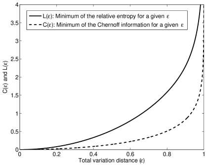
Figure 1: A plot of the minima of the Chernoff information and the relative entropy for a given total variation distance $\varepsilon\in[0,1]$, denoted by $C(\varepsilon)$ and $L(\varepsilon)$, respectively; $C$ and $L$ are provided, respectively, in Proposition 2 and [13, Theorem 2] or [23, Eq. (59)] (see (26)).

Figure 1 plots these minima as a function of the total variation distance. For small values of $\varepsilon$, $C(\varepsilon)$ and $L(\varepsilon)$, respectively, are approximately equal to $\frac{\varepsilon^{2}}{2}$ and $2\varepsilon^{2}$ (note that Pinsker’s inequality is tight for $\varepsilon\ll 1$), so

$$\lim_{\varepsilon\rightarrow 0}\frac{L(\varepsilon)}{C(\varepsilon)}=4.$$

Discussion 2

The lower bound on the capacitory discrimination in (15), expressed in terms of the total variation distance, forms a closed-form expression of the bound by Topsøe in [25, Theorem 5]. The bound in [25] is

$$\overline{C}(P,Q)\geq\sum_{\nu=1}^{\infty}\frac{\bigl{(}d_{\text{TV}}(P,Q)\bigr{)}^{2\nu}}{\nu(2\nu-1)}.$$ (28)

The equivalence of (15) and (28) follows from the power series expansion of the binary entropy function

$$h(x)=\log 2-\sum_{\nu=1}^{\infty}\frac{(1-2x)^{2\nu}}{2\nu(2\nu-1)},\quad\forall\,x\in[0,1]$$

which yields that

$$\sum_{\nu=1}^{\infty}\frac{\bigl{(}d_{\text{TV}}(P,Q)\bigr{)}^{2\nu}}{\nu(2\nu-1)} =2\left[\log 2-h\left(\frac{1-d_{\text{TV}}(P,Q)}{2}\right)\right]$$

$$=2d\left(\frac{1-d_{\text{TV}}(P,Q)}{2}\,\big{|}\big{|}\,\frac{1}{2}\right)$$

where $d(\cdot||\cdot)$ is defined in (16). Note, however, that the proof here is more simple than the proof of [25, Theorem 5] (which relies on properties of the triangular discrimination in [25] and previous theorems of this paper), and it also leads directly to a closed-form expression of this bound. Consequently, one concludes that the lower bound in [25, Theorem 5] is a special case of Theorem 6 (see [14] and [16, Corollary 5.4]), which provides a lower bound on a symmetric $f$-divergence in terms of the total variation distance.

IV A Bound for Lossless Source Coding

We illustrate in the following a use of Proposition 4 for the derivation of an improved and refined bound for lossless source coding. This tightens, and also refines under a certain condition, a bound by Csiszár [7].

Consider a memoryless and stationary source with alphabet $\mathcal{U}$ that emits symbols according to a probability distribution $P$, and assume that a uniquely decodable (UD) code with an alphabet of size $d$ is used. It is well known that such a UD code achieves the entropy of the source if and only if the length $l(u)$ of the codeword that is assigned to each symbol $u\in\mathcal{U}$ satisfies the equality

$$l(u)=-\log_{d}P(u),\quad\forall\,u\in\mathcal{U}.$$

This corresponds to a dyadic source where, for every $u\in\mathcal{U}$, we have $P(u)=d^{-n_{u}}$ with a natural number $n_{u}$; in this case, $l(u)=n_{u}$ for every symbol $u\in\mathcal{U}$. Let $\overline{L}\triangleq{\rm I\!E}[L]$ designate the average length of the codewords, and $H_{d}(U)\triangleq-\sum_{u\in\mathcal{U}}P(u)\,\log_{d}P(u)$ be the entropy of the source (to the base $d$). Furthermore, let $c_{d,l}\triangleq\sum_{u\in\mathcal{U}}d^{-l(u)}.$ According to the Kraft-McMillian inequality (see [5, Theorem 5.5.1]), the inequality $c_{d,l}\leq 1$ holds in general for UD codes, and the equality $c_{d,l}=1$ holds if the code achieves the entropy of the source (i.e., $\overline{L}=H_{d}(U)$).

Define a probability distribution $Q_{d,l}$ by

$$Q_{d,l}(u)\triangleq\left(\frac{1}{c_{d,l}}\right)\,d^{-l(u)},\quad\forall\,u\in\mathcal{U}$$ (29)

and let $\Delta_{d}\triangleq\overline{L}-H_{d}(U)$ designate the average redundancy of the code. Note that for a UD code that achieves the entropy of the source, its probability distribution $P$ is equal to $Q_{d,l}$ (since $c_{d,l}=1$, and $P(u)=d^{-l(u)}$ for every $u\in\mathcal{U}$).

In [7], a generalization for UD source codes has been studied by a derivation of an upper bound on the $L_{1}$ norm between the two probability distributions $P$ and $Q_{d,l}$ as a function of the average redundancy $\Delta_{d}$ of the code. To this end, straightforward calculation shows that the relative entropy from $P$ to $Q_{d,l}$ is given by

$$D(P||Q_{d,l})=\Delta_{d}\,\log d+\log\bigl{(}c_{d,l}\bigr{)}.$$ (30)

The interest in [7] is in getting an upper bound that only depends on the average redundancy $\Delta_{d}$ of the code, but is independent of the distribution of the lengths of the codewords. Hence, since the Kraft-McMillian inequality states that $c_{d,l}\leq 1$ for general UD codes, it is concluded in [7] that

$$D(P||Q_{d,l})\leq\Delta_{d}\,\log d.$$ (31)

Consequently, it follows from Pinsker’s inequality that

$$\sum_{u\in\mathcal{U}}\bigl{|}P(u)-Q_{d,l}(u)\bigr{|}\leq\min\bigl{\{}\sqrt{2\Delta_{d}\log d},\,2\bigr{\}}$$ (32)

since also, from the triangle inequality, the sum on the left-hand side of (32) cannot exceed 2. This inequality is indeed consistent with the fact that the probability distributions $P$ and $Q_{d,l}$ coincide when $\Delta_{d}=0$ (i.e., for a UD code that achieves the entropy of the source).

At this point we deviate from the analysis in [7]. One possible improvement of the bound in (32) follows by replacing Pinsker’s inequality with the result in [13], i.e., by taking into account the exact parametrization of the infimum of the relative entropy for a given total variation distance. This gives the following tightened bound:

$$\sum_{u\in\mathcal{U}}\bigl{|}P(u)-Q_{d,l}(u)\bigr{|}\leq 2\;L^{-1}(\Delta_{d}\log d)$$ (33)

where $L^{-1}$ is the inverse function of $L$ in (26) (it is calculated numerically).

In the following, the utility of Proposition 4 is shown by refining the latter bound in (33). Let

$$\delta(u)\triangleq l(u)+\log_{d}P(u),\quad\forall\,u\in\mathcal{U}.$$

Calculation of the dual divergence gives

$$D(Q_{d,l}||P)$$

$$=\log d\,\sum_{u\in\mathcal{U}}Q_{d,l}(u)\log_{d}\left(\frac{Q_{d,l}(u)}{P(u)}\right)$$

$$=\log d\,\left[-\frac{\log_{d}(c_{d,l})}{c_{d,l}}\sum_{u\in\mathcal{U}}d^{-l(u)}-\frac{1}{c_{d,l}}\sum_{u\in\mathcal{U}}l(u)d^{-l(u)}-\frac{1}{c_{d,l}}\sum_{u\in\mathcal{U}}\log_{d}P(u)\;d^{-l(u)}\right]$$

$$=-\log(c_{d,l})-\frac{\log d}{c_{d,l}}\sum_{u\in\mathcal{U}}\delta(u)\,d^{-l(u)}$$

$$=-\log\bigl{(}c_{d,l}\bigr{)}-\frac{\log d}{c_{d,l}}\,\sum_{u\in\mathcal{U}}P(u)\,\delta(u)\,d^{-\delta(u)}$$

$$=-\log\bigl{(}c_{d,l}\bigr{)}-\left(\frac{\log d}{c_{d,l}}\right){\rm I\!E}\bigl{[}\delta(U)\,d^{-\delta(U)}\bigr{]}$$ (34)

and the combination of (17), (30) and (34) yields that

$$J(P,Q_{d,l})=\frac{1}{2}\left[\Delta_{d}\log d-\left(\frac{\log d}{c_{d,l}}\right){\rm I\!E}\bigl{[}\delta(U)\,d^{-\delta(U)}\bigr{]}\right].$$ (35)

In the continuation of this analysis, we restrict our attention to UD codes that satisfy the condition

$$l(u)\geq\left\lceil\log_{d}\frac{1}{P(u)}\right\rceil,\quad\forall\,u\in\mathcal{U}.$$ (36)

In general, it excludes Huffman codes; nevertheless, it is satisfied by some other important UD codes such as the Shannon code, Shannon-Fano-Elias code, and arithmetic coding (see, e.g., [5, Chapter 5]). Since (36) is equivalent to the condition that $\delta$ is non-negative on $\mathcal{U}$, it follows from (35) that

$$J(P,Q_{d,l})\leq\frac{\Delta_{d}\log d}{2}$$ (37)

so, the upper bound on Jeffreys’ divergence in (37) is twice smaller than the upper bound on the relative entropy in (31). It is partially because the term $\log c_{d,l}$ is canceled out along the derivation of the bound in (37), in contrast to the derivation of the bound in (31) where this term was upper bounded by zero (hence, it has been removed from the bound) in order to avoid its dependence on the length of the codeword for each individual symbol.

Following Proposition 4, for $x\geq 0$, let $\varepsilon\triangleq\varepsilon(x)$ be the unique solution in the interval $[0,1)$ of the equation

$$\varepsilon\,\log\left(\frac{1+\varepsilon}{1-\varepsilon}\right)=x.$$ (38)

The combination of (19) and (37) implies that

$$\sum_{u\in\mathcal{U}}\bigl{|}P(u)-Q_{d,l}(u)\bigr{|}\leq 2\;\varepsilon\left(\frac{\Delta_{d}\log d}{2}\right).$$ (39)

The bounds in (32), (33) and (39) are depicted in Figure 2 for UD codes where the size of their alphabet is $d=10$.

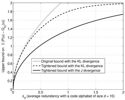
Figure 2: Upper bounds on $\sum|P(u)-Q_{d,l}(u)|$ as a function of the average redundancy $\Delta_{d}\triangleq{\rm I\!E}[L]-H_{d}$ for a UD code with an alphabet of size $d=10$. The original bound in (32) appears in [7], and the tightened bound that relies on the Kullback-Leibler (KL) divergence is given in (33). The further tightening of this bound is restricted in this plot to UD codes whose codewords satisfy the condition in (36). The latter bound relies on Proposition 4 for Jeffreys’ (J) divergence, and it is given in (39).

In the following, the bounds in (33) and (39) are compared analytically for the case where the average redundancy is small (i.e., $\Delta_{d}\approx 0$). Under this approximation, the bound in (32) (i.e., the original bound from [7]) coincides with its tightened version in (33). On the other hand, since for $\varepsilon\approx 0$, the left-hand side of (38) is approximately $2\varepsilon^{2}$, it follows from (38) that, for $x\approx 0$, we have $\varepsilon(x)\approx\sqrt{\frac{x}{2}}.$ It follows that, if $\Delta_{d}\approx 0$, inequality (39) gets approximately the form

$$\sum_{u\in\mathcal{U}}\bigl{|}P(u)-Q_{d,l}(u)\bigr{|}\leq\sqrt{\Delta_{d}\log d}.$$

Hence, even for a small average redundancy, the bound in (39) improves (32) by a factor of $\sqrt{2}$. This conclusion is consistent with the plot in Figure 2.

References

- [1] S. M. Ali and S. D. Silvey, “A general class of coefficients of divergence of one distribution from another,” Journal of the Royal Statistics Society, series B, vol. 28, no. 1, pp. 131–142, 1966.
- [2] M. Basseville, “Divergence measures for statistical data processing - an annotated bibliography,” Signal Processing, vol. 93, no. 4, pp. 621–633, 2013.
- [3] J. Briët and P. Harremoës, “Properties of classical and quantum Jensen-Shannon divergence,” Physical Review A, vol. 79, 052311, May 2009.
- [4] J. Burbea and C. R. Rao, “On the convexity of some divergence measures based on entropy functions,” IEEE Trans. on Information Theory, vol. 28, no. 3, pp. 489–495, May 1982.
- [5] T. M. Cover and J. A. Thomas, Elements of Information Theory, John Wiley and Sons, second edition, 2006.
- [6] I. Csiszár, “Information-type measures of difference of probability distributions and indirect observations,” Studia Scientiarum Mathematicarum Hungarica, vol. 2, pp. 299–318, 1967.
- [7] I. Csiszár, “Two remarks to noiseless coding,” Information and Control, vol. 11, no. 3, pp. 317–322, September 1967.
- [8] I. Csiszár and J. Körner, Information Theory: Coding Theorems for Discrete Memoryless Systems, second edition, Cambridge University Press, 2011.
- [9] I. Csiszár and P. C. Shields, Information Theory and Statistics: A Tutorial, Foundations and Trends in Communications and Information Theory, vol. 1, no. 4, pp. 417–528, 2004.
- [10] S. S. Dragomir, Inequalities for Csiszár -Divergences in Information Theory, RGMIA Monographs, Victoria University, 2000. [Online]. Available: http://rgmia.org/monographs/csiszar.htm.
- [11] D. M. Endres and J. E. Schindelin, “A new metric for probability distributions,” IEEE Trans. on Information Theory, vol. 49, no. 7, pp. 1858–1860, July 2003.
- [12] T. van Erven and P. Harremoës, “Rényi divergence and Kullback-Leibler divergence,” IEEE Trans. on Information Theory, vol. 60, no. 7, pp. 3797–3820, July 2014.
- [13] A. A. Fedotov, P. Harremoës and F. Topsøe, “Refinements of Pinsker’s inequality,” IEEE Trans. on Information Theory, vol. 49, no. 6, pp. 1491–1498, June 2003.
- [14] G. L. Gilardoni, “On the minimum -divergence for given total variation,” Comptes Rendus Mathematique, vol. 343, no. 11–12, pp. 763–766, 2006.
- [15] G. L. Gilardoni, “On Pinsker’s and Vajda’s type inequalities for Csiszár’s -divergences,” IEEE Trans. on Information Theory, vol. 56, no. 11, pp. 5377–5386, November 2010.
- [16] A. Guntuboyina, S. Saha, and G. Schiebinger, “Sharp inequalities for -divergences,” IEEE Trans. on Information Theory, vol. 60, no. 1, pp. 104–121, January 2014.
- [17] H. Jeffreys, “An invariant form for the prior probability in estimation problems,” Proceedings of the Royal Society A, vol. 186, no. 1007, pp. 453–461, September 1946.
- [18] T. Kailath, “The divergence and Bhattacharyya distance measures in signal selection,” IEEE Trans. on Communication Technology, vol. 15, no. 1, pp. 52–60, February 1967.
- [19] C. Kraft, “Some conditions for consistency and uniform consistency of statistical procedures,” University of California Publications in Statistics, vol. 1, pp. 125–142, 1955.
- [20] F. Liese and I. Vajda, “On divergences and informations in statistics and information theory,” IEEE Trans. on Information Theory, vol. 52, no. 10, pp. 4394–4412, October 2006.
- [21] J. Lin, “Divergence measures based on the Shannon entropy,” IEEE Trans. on Information Theory, vol. 37, no. 1, pp. 145–151, Jan. 1991.
- [22] T. Morimoto, “Markov processes and the -theorem,” Journal of the Physical Society of Japan, vol. 18, no. 3, pp. 328–331, 1963.
- [23] M. D. Reid and R. C. Williamson, “Information, divergence and risk for binary experiments,” Journal of Machine Learning Research, vol. 12, pp. 731–817, March 2011.
- [24] I. Sason, “An information-theoretic perspective of the Poisson approximation via the Chen-Stein method,” un-published manuscript, arXiv:1206.6811v4, 2012.
- [25] F. Topsøe, “Some inequalities for information divergence and related measures of discrimination,” IEEE Trans. on Information Theory, vol. 46, pp. 1602–1609, July 2000.
- [26] A. D. Yardi. A. Kumar, and S. Vijayakumaran, “Channel-code detection by a third-party receiver via the likelihood ratio test,” Proceedings of the 2014 IEEE International Symposium on Information Theory, pp. 1051–1055, Honolulu, Hawaii, USA, July 2014.