A Unified Framework of Constrained Regression

Abstract

Generalized additive models (GAMs) play an important role in modeling and understanding complex relationships in modern applied statistics. They allow for flexible, data-driven estimation of covariate effects. Yet researchers often have a priori knowledge of certain effects, which might be monotonic or periodic (cyclic) or should fulfill boundary conditions. We propose a unified framework to incorporate these constraints for both univariate and bivariate effect estimates and for varying coefficients. As the framework is based on component-wise boosting methods, variables can be selected intrinsically, and effects can be estimated for a wide range of different distributional assumptions. Bootstrap confidence intervals for the effect estimates are derived to assess the models. We present three case studies from environmental sciences to illustrate the proposed seamless modeling framework. All discussed constrained effect estimates are implemented in the comprehensive R package mboost for model-based boosting.

1 Introduction

When statistical models are used, certain assumptions are made, either for convenience or to incorporate the researchers’ assumptions on the shape of effects, e.g., because of prior knowledge. A common, yet very strong assumption in regression models is the linearity assumption. The effect estimate is constrained to follow a straight line. Despite the widespread use of linear models, it often may be more appropriate to relax the linearity assumption.

Let us consider a set of observations $(y_{i},\bm{x}^{\top}_{i}),i=1,\ldots,n,$ where $y_{i}$ is the response variable and $\bm{x}_{i}=(x_{i}^{(1)},\ldots,x_{i}^{(L)})^{\top}$ consists of $L$ possible predictors of different nature, such as categorical or continuous covariates. To model the dependency of the response on the predictor variables, we consider models with structured additive predictor $\eta(\bm{x})$ of the form

$$\eta(\bm{x})=\beta_{0}+\sum_{l=1}^{L}f_{l}(\bm{x}),$$ (1)

where the functions $f_{l}(\cdot)$ depend on one or more predictors contained in $\bm{x}$. Examples include linear effects, categorical effects, and smooth effects. More complex models with functions that depend on multiple variables such as random effects, varying coefficients, and bivariate effects, can be expressed in this framework as well (for details, see Fahrmeir et al 2004).

Structured additive predictors can be used in different types of regression models. For example, replacing the linear predictor of a generalized linear model with (1) yields a structured additive regression (STAR) model, where $\mathds{E}(y|\bm{x})=h(\eta(\bm{x}))$ with (known) response function $h$. However, structured additive predictors can be used much more generally, in any class of regression models (as we will demonstrate in one of our applications in a conditional transformation model that allows to describe general distributional features and not only the mean in terms of covariates).

A convenient way to fit models with structured additive predictors is given by component-wise functional gradient descent boosting (Bühlmann and Yu 2003), which minimizes an empirical risk function with the aim to optimize prediction accuracy. In case of structured additive regression, the risk will usually correspond to the negative log-likelihood but more general types of risks can be defined for example for quantile regression models (Fenske et al 2011), or in the context of conditional transformation models (Hothorn et al 2014b). The boosting algorithm is especially attractive due to its intrinsic variable selection properties (Kneib et al 2009, Hofner et al 2011a) and the ease of combining a wide range of modeling alternatives in a single model specification. Furthermore, a single estimation framework can be used for a very wide range of distributional assumptions or even in distribution free approaches. Thus, boosting models are not restricted to exponential family distributions.

Models with structured additive predictors offer great flexibility but typically result in smooth yet otherwise unconstrained effect estimates $\hat{f}_{l}$. To overcome this, we propose a framework to fit models with constrained structured additive predictors based on boosting methods. We derive cyclic effects in the boosting context and improved fitting methods for monotonic P-splines. Bootstrap-confidence intervals are proposed to assess the fitted models.

1.1 Application of Constrained Models

In the first case study presented, we model the effect of air pollution on daily mortality in São Paulo (Section 7.1). Additionally, we control for environmental conditions (temperature, humidity) and model both the seasonal pattern and the long-term trend. Furthermore, we consider the effect of the pollutant of interest, SO₂. In modeling the seasonal pattern of mortality related to air pollution, the effect should be continuous over time, and huge jumps for effects only one day apart would be unrealistic. Thus, the first and last days of the year should be continuously joined. Hence, we use smooth functions with a cyclic constraint (Section 3.2). This has two effects. First, it allows us to fit a plausible model as we avoid jumps at the boundaries. Second, the estimation at the boundaries is stabilized as we exploit the cyclic nature of the data.

From a biological point of view, it seems reasonable to expect an increase in mortality with increasing concentration of the pollutant SO₂. Linear effects are monotonic but do not offer enough flexibility in this case. Smooth effects, on the other hand, offer more flexibility, but monotonicity might be violated. To bridge this gap, smooth monotonic effects can be used (Sec. 3.3). Additionally to the proposed boosting framework, we will use the framework for constrained structured additive models of Pya and Wood (2014) (which is similar to ours but is restricted to exponential family distributions) for comparison in the first case study.

In a second case study, we aim at modeling the activity of roe deer in Bavaria, Germany, given environmental conditions, such as temperature, precipitation, and depth of snow; animal-specific variables, such as age and sex; and a temporal component. The latter reflects the animals’ day/night rhythm as well as seasonal patterns. We model the temporal effect as a smooth bivariate effect as the days change throughout the year, i.e., the solar altitude changes in the course of a day and with the seasons. Cyclic constraints for both variables (time of the day and calendar day) should be used. Hence, we have a bivariate periodic effect $f(t_{\text{hours}},t_{\text{days}})$ (Section 4.2). As male and female animals differ strongly in their temporal activity profiles, we additionally use sex as a binary effect modifier $f(t_{\text{hours}},t_{\text{days}})I_{(\text{sex = male})}$, i.e., we have a varying coefficient surface with a cyclicity constraint for the smooth bivariate effect. Additionally, the effects of environmental variables are allowed to smoothly vary over time but are otherwise unconstrained.

In a third case study, we go beyond a model for the mean activity by modeling the conditional distribution of a surrogate of roe deer activity: the number of deer–vehicle collisions per day. In the framework of conditional transformation models (Hothorn et al 2014b), we fit daily distributions of the number of such collisions and penalize differences in these distributions between subsequent days. A monotonic constraint is needed to fit the conditional distribution, while a cyclic constraint should be used for the seasonal effect of deer–vehicle collisions. These two conditions yield a tensor product of two univariate constrained effects.

1.2 Overview of the Paper

Model estimation based on boosting is briefly introduced in Section 2. Monotonic effects, cyclic P-splines, and P-splines with boundary constraints are introduced in Section 3, where we also introduce varying coefficients. An extension of monotonicity and cyclicity constraints to bivariate P-splines is given in Section 4. In Section 5 we sketch inferential procedures and derive bootstrap confidence intervals for the constrained boosting framework. Computational details can be found in Section 6. We present the three case studies described above in Section 7. An overview of past and present developments of constrained regression models is given in Online Resource 1 (Section LABEL:sec:overview). The definition of the Kronecker product and element-wise matrix product is given in Online Resource 1 (Section LABEL:sec:matrix-algebra). Details on the São Paulo air pollution data set and the model specification is given in Online Resource 1 (Section LABEL:sec:sao_paulo_data), while Online Resource 1 (Section LABEL:sec:roedeer_data) gives details on the Bavarian roe deer data and the specification used to model the activity of roe deer. Online Resource 1 (Section LABEL:sec:simulation_study) gives an empirical evaluation of the proposed methods. R code to reproduce the fitted models from our case studies is given as electronic supplement.

2 Model Estimation Based on Boosting

To fit a model with structured additive predictor (1) by component-wise boosting (Bühlmann and Yu 2003), one starts with a constant model, e.g., $\hat{\eta}(\mathbf{x})\equiv 0$, and computes the negative gradient $\mathbf{u}=(u_{1},\dots,u_{n})^{\top}$ of the loss function evaluated at each observation. An appropriate loss function is guided by the fitting problem. For Gaussian regression models, one may use the quadratic loss function, and for generalized linear models, the negative log-likelihood. In the Gaussian regression case, the negative gradient $\mathbf{u}$ equals the standard residuals; in other cases, $\mathbf{u}$ can be regarded as “working residuals”. In the next step, each model component $f_{l},\,l=1,\dots,L,$ of the structured additive model (1) is fitted separately to the negative gradient $\mathbf{u}$ by penalized least-squares. Only the model component that best describes the negative gradient is updated by adding a small proportion of its fit (e.g., $10\%$) to the current model fit. New residuals are computed, and the whole procedure is iterated until a fixed number of iterations is reached. The final model $\hat{\eta}(\mathbf{x})$ is defined as the sum of all models fitted in this process. As only one modeling component is updated in each boosting iteration, variables are selected by stopping the boosting procedure after an appropriate number of iterations. This is usually done using cross-validation techniques.

For each of the model components, a corresponding regression model that is applied to fit the residuals has to be specified, the so-called base-learner. Hence, the base-learners resemble the model components $f_{l}$ and determine which functional form each of the components can take. In the following sections, we introduce base-learners for smooth effect estimates and derive special base-learners for fitting constrained effect estimates. These can then be directly used within the generic model-based boosting framework without the need to alter the general algorithm. For details on functional gradient descent boosting and specification of base-learners, see Bühlmann and Hothorn (2007) and Hofner et al (2014b).

3 Constrained Regression

3.1 Estimating Smooth Effects

For the sake of simplicity in the remainder of this paper, we will consider an arbitrary continuous predictor $x$ and a single base-learner $f_{l}$ only when we drop the function index $l$. To model smooth effects of continuous variables, we utilized penalized B-splines (i.e., P-splines). These were introduced by Eilers and Marx (1996) for nonparametric regression and were later transferred to the boosting framework by Schmid and Hothorn (2008). Considering observations $\mathbf{x}=(x_{1},\ldots,x_{n})^{\top}$ of a single variable $x$, a non-linear function $f(x)$ can be approximated as

$$f(x)=\sum_{j=1}^{J}\beta_{j}B_{j}(x;\delta)=\mathbf{B}(x)^{\top}\bm{\beta},$$

where $B_{j}(\cdot;\delta)$ is the $j$th B-spline basis function of degree $\delta$. The basis functions are defined on a grid of $J-(\delta-1)$ inner knots $\xi_{1},\ldots,\xi_{J-(\delta-1)}$ with additional boundary knots (and usually a knot expansion in the boundary knots) and are combined in the vector $\mathbf{B}(x)=(B_{1}(x),\dots,B_{J}(x))^{\top}$, where for simplicity $\delta$ was dropped. For more details on the construction of B-splines, we refer the reader to Eilers and Marx (1996). The function estimates can be written in matrix notation as $\hat{f}(\mathbf{x})=\mathbf{B}\hat{\bm{\beta}}$, where the design matrix $\mathbf{B}=(\mathbf{B}(x_{1}),\ldots,\mathbf{B}(x_{n}))^{\top}$ comprises the B-spline basis vectors $\mathbf{B}(x)$ evaluated for each observation $x_{i}$, $i=1,\ldots,n$. The function estimate $\hat{f}(\mathbf{x})$ might adapt the data too closely and might become too erratic. To enforce smoothness of the function estimate, an additional penalty is used that penalizes large differences of the coefficients of adjacent knots. Hence, for a continuous response $\mathbf{u}$ (here the negative gradient vector), we can estimate the function by minimizing a penalized least-squares criterion

$$\mathcal{Q}(\bm{\beta})=(\mathbf{u}-\mathbf{B}\bm{\beta})^{\top}(\mathbf{u}-\mathbf{B}\bm{\beta})+\lambda\mathcal{J}(\bm{\beta};d),$$ (2)

where $\lambda$ is the smoothing parameter that governs the trade-off between smoothness and closeness to the data. We use a quadratic difference penalty of order $d$ on the coefficients , i.e., $\mathcal{J}(\bm{\beta};d)=\sum_{j}(\Delta^{d}\beta_{j})^{2}$, with $\Delta^{1}\beta_{j}=\Delta\beta_{j}:=\beta_{j}-\beta_{j-1}$. By applying the $\Delta$ operator recursively we get $\Delta^{2}\beta_{j}=\Delta(\Delta\beta_{j})=\beta_{j}-2\beta_{j-1}+\beta_{j-2}$, etc. In matrix notation the penalty can be written as

$$\mathcal{J}(\bm{\beta};d)=\bm{\beta}^{\top}\mathbf{D}_{(d)}^{\top}\mathbf{D}_{(d)}\bm{\beta}.$$ (3)

The difference matrices $\mathbf{D}_{(d)}$ are constructed such that they lead to the appropriate differences: first- and second-order differences result from matrices of the form

$$\mathbf{D}_{(1)}=\begin{pmatrix}-1&1&&\\ &\ddots&\ddots&\\ &&-1&1\\ \end{pmatrix}$$ (4)

and

$$\mathbf{D}_{(2)}=\begin{pmatrix}1&-2&1&&\\ &\ddots&\ddots&\ddots&\\ &&1&-2&1\\ \end{pmatrix},$$ (5)

where empty cells are equal to zero. Higher order difference penalties can be easily derived. Difference penalties of order one penalize the deviation from a constant. Second-order differences penalize the deviation from a straight line. In general, differences of order $d$ penalize deviations from polynomials of order $d-1$. The unpenalized effects, i.e., the constant (d = 1) or the straight line (d = 2) are called the null space of the penalty. The null space remains unpenalized, even in the limit of $\lambda\rightarrow\infty$.

The penalized least-squares criterion (2) is optimized in each boosting step irrespective of the underlying distribution assumption. The distribution assumption, or more generally, a specific loss function, is only used to derive the appropriate negative gradient of the loss function.To fit the negative gradient vector $\mathbf{u}$, we fix the smoothing parameter $\lambda$ separately for each base-learner such that the corresponding degrees of freedom of the base-learner are relatively small (typically not more than 4 to 6 degrees of freedom). The boosting algorithm iteratively updates one base-learner per boosting iteration. As the same base-learner can enter the model multiple times, the final effect, which is the sum of all effect estimates for this base-learner, can adapt to arbitrarily higher order smoothness. For details see Bühlmann and Yu (2003) and Hofner et al (2011a).

3.2 Estimating Cyclic Smooth Effects

P-splines with a cyclic constraint (Eilers and Marx 2010) can be used to model periodic, seasonal data. The cyclic B-spline basis functions are constructed without knot expansion (Figure 1). The B-splines are “wrapped” at the boundary knots. The boundary knots $\xi_{0}$ and $\xi_{J}$ (equal to $\xi_{12}$ in Fig. 1) play a central role in this setting as they specify the points where the function estimate should be smoothly joined. If $x$ is, for example, the time during the day, then $\xi_{0}$ is 0:00, whereas $\xi_{J}$ is 24:00. Defining the B-spline basis in this fashion leads to a cyclic B-spline basis with the $(n\times(J+1))$ design matrix $\mathbf{B}_{\text{cyclic}}$. The corresponding coefficients are collected in the $((J+1)\times 1)$ vector $\bm{\beta}=(\beta_{0},\ldots,\beta_{J})$.

Figure 1: Illustration of cyclic P-splines of degree three, with 11 inner knots and boundary knots $\xi_{0}$ and $\xi_{12}$. The gray curves correspond to B-splines. The black curves correspond to B-splines that are “wrapped” at the boundary knots, leading to a cyclic representation of the function. The dashed B-spline basis depends on observations in $[\xi_{9},\xi_{12}]\cup[\xi_{0},\xi_{1}]$ and thus on observations from both ends of the range of the covariate. The same holds for the other two black B-spline curves (solid and dotted).

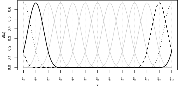
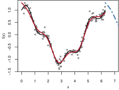
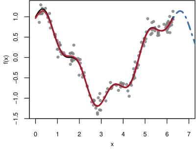
Specifying a cyclic basis guarantees that the resulting function estimate is continuous in the boundary knots. However, no smoothness constraint is imposed so far. This can be achieved by a cyclic difference penalty, for example, $\mathcal{J}_{\text{cyclic}}(\bm{\beta})=\sum_{j=0}^{J}(\beta_{j}-\beta_{j-1})^{2}$ (with $d=1$) or $\mathcal{J}_{\text{cyclic}}(\bm{\beta})=\sum_{j=0}^{J}(\beta_{j}-2\beta_{j-1}+\beta_{j-2})^{2}$ (with $d=2$), where the index $j$ is “wrapped”, i.e., $j:=J+1+j$ if $j<0$. Thus, the differences between $\beta_{0}$ and $\beta_{J}$ or even $\beta_{J-1}$ are taken into account for the penalty. Hence, the boundaries of the support are stabilized, and smoothness in and around the boundary knots is enforced. This can also be seen in Figure 2. The non-cyclic estimate (Fig. 2) is less stable at the boundaries. As a consequence, the ends do not meet. The cyclic estimate (Fig. 2), in contrast, is stabilized at the boundaries, and the ends are smoothly joined.

(a)

(b)

Figure 2: 2 Non-cyclic and 2 cyclic P-splines. The red curve is the function estimated P-spline function. The blue, dashed curve is the same function shifted one period to the right. The data were simulated from a cyclic function with period $2\pi$: $f(x)=\cos(x)+0.25\sin(4x)$ (black line) and realizations with additional normally distributed errors ($\sigma=0.1$; gray dots). The cyclic estimate is closer to the true function and more stable in the boundary regions, and the ends meet (see 2 at $x=2\pi$).

In matrix notation the penalty can be written as

$$\mathcal{J}_{\text{cyclic}}(\bm{\beta};d)=\bm{\beta}^{\top}\widetilde{\mathbf{D}}^{\top}_{(d)}\widetilde{\mathbf{D}}_{(d)}\bm{\beta},$$ (6)

with difference matrices

$$\widetilde{\mathbf{D}}_{(1)}=\begin{pmatrix}1&&&-1\\ -1&1&&\\ &\ddots&\ddots&\\ &&-1&1\\ \end{pmatrix}$$ (7)

and

$$\widetilde{\mathbf{D}}_{(2)}=\begin{pmatrix}1&&&1&-2\\ -2&1&&&1\\ 1&-2&1&&\\ &\ddots&\ddots&\ddots&\\ &&1&-2&1\\ \end{pmatrix},$$ (8)

where empty cells are equal to zero. Coefficients can then be estimated using the penalized least-squares criterion (2), where the design matrix and the penalty matrix are replaced with the corresponding cyclic counterparts, i.e., $\mathcal{Q}(\bm{\beta})=(\mathbf{u}-\mathbf{B}_{\text{cyclic}}\,\bm{\beta})^{\top}(\mathbf{u}-\mathbf{B}_{\text{cyclic}}\,\bm{\beta})+\lambda\mathcal{J}_{\text{cyclic}}(\bm{\beta};d)$. Again, we fix the smoothing parameter $\lambda$ and control the smoothness of the final fit by the number of boosting iterations.

As mentioned in Section 3.1, P-splines have a null space, i.e., an unpenalized effect, which depends on the order of the differences in the penalty. However, cyclic P-splines have a null space that includes only a constant, irrespective of the order of the difference penalty. Globally seen, i.e., for the complete function estimate, the order of the penalty plays no role (even in the limit $\lambda\rightarrow\infty$). Locally, however, the order of the difference penalty has an effect. For example, with $d=2$, the estimated function is penalized for deviations from linearity and hence, locally approaches a straight line (with increasing $\lambda$).

An empirical evaluation of cyclic P-splines shows the clear superiority of cyclic splines compared to unconstrained estimates, both with respect to the MSE and the conformance with the cyclicity assumption (Online Resource 1; Section LABEL:sec:sim_cyclic-effects).

3.3 Estimating Monotonic Effects

To achieve a smooth, yet monotonic function estimate, Eilers (2005) introduced P-splines with an additional asymmetric difference penalty. The penalized least-squares criterion (2) becomes

$$\begin{split}\mathcal{Q}(\bm{\beta})=&(\mathbf{u}-\mathbf{B}\bm{\beta})^{\top}(\mathbf{u}-\mathbf{B}\bm{\beta})+\lambda_{1}\mathcal{J}(\bm{\beta};d)\\ &+\lambda_{2}\mathcal{J}_{\text{asym}}(\bm{\beta};c),\end{split}$$ (9)

with the quadratic difference penalty $\mathcal{J}(\bm{\beta};d)$ as in standard P-splines (Eq. 3) and an additional asymmetric difference penalty of order $c$

$$\mathcal{J}_{\text{asym}}(\bm{\beta};c)=\sum_{j=c+1}^{J}v_{j}(\Delta^{c}\beta_{j})^{2}=\bm{\beta}^{\top}\mathbf{D}_{(c)}^{\top}\mathbf{V}\mathbf{D}_{(c)}\bm{\beta},$$ (10)

where the difference matrix $\mathbf{D}_{(c)}$ is constructed as in Equations (4) and (5). This asymmetric difference penalty ensures that the differences (of order $c$) of adjacent coefficients are positive or negative. The choice of $c$ implies the type of the additional constraint: monotonicity for $c=1$ or convexity/concavity for $c=2$. In the remainder of this article, we restrict our attention to monotonicity constraints; however, one can also consider concave constraints. The asymmetric penalty looks very much like the P-spline penalty (3) with the important distinction of weights $v_{j}$, which are specified as

$$v_{j}=\begin{cases}0&\text{if \, $\Delta^{c}\beta_{j}>0$}\\ 1&\text{if \, $\Delta^{c}\beta_{j}\leq 0$}.\end{cases}$$ (11)

The weights are collected in the diagonal matrix $\mathbf{V}=\operatorname{diag}(\mathbf{v})$. With $c=1$, this enforces monotonically increasing functions. Changing the direction of the inequalities in the distinction of cases leads to monotonically decreasing functions. Note that positive/negative differences of adjacent coefficients are sufficient but not necessary for monotonically increasing/decreasing effects. As the weights (11) depend on the coefficients $\bm{\beta}$, a solution to (9) can only be found by iteratively minimizing $\mathcal{Q}(\bm{\beta})$ with respect to $\bm{\beta}$, where the weights $\mathbf{v}$ are updated in each iteration. The estimation converges if no further changes in the weight matrix $\mathbf{V}$ occur. The penalty parameter $\lambda_{2}$, which is associated with the additional constraint (10), should be chosen quite large (e.g., $10^{6}$; Eilers 2005) and resembles the researcher’s a priori assumption of monotonicity. Larger values are associated with a stronger impact of the monotonic constraint on the estimation. The penalty parameter $\lambda_{1}$ associated with the smoothness constraint is usually fixed so that the overall degrees of freedom of the smooth monotonic effect resemble a pre-specified value. Again, by updating the base-learner multiple times, the effect can adapt greater flexibility while keeping the monotonicity assumption. A detailed discussion of monotonic P-splines in the context of boosting models is given in Hofner et al (2011b). In their presented framework, the authors also derive an asymmetric difference penalty for monotonicity-constrained, ordered categorical effects.

One can also use asymmetric difference penalties on differences of order 0, i.e., on the coefficients themselves, to achieve smooth positive or negative effect estimates. This idea can also be used to fit smooth effect estimates with an arbitrarily fixed co-domain by specifying either upper or lower bounds or both bounds at the same time.

Improved Fitting Method for Monotonic Effects

An alternative to iteratively minimizing the penalized least-squares criterion (9) to obtain smooth monotonic estimates, is given by quadratic programming methods (Goldfarb and Idnani 1982, 1983). To fit the monotonic base-learner to the negative gradient vector $\mathbf{u}$ using quadratic programming, we minimize the penalized least-squares criterion (2) with the additional constraint

$$\mathbf{D}_{(c)}\bm{\beta}\geq\bm{0},$$

with difference matrix $\mathbf{D}_{(c)}$ as defined above and null vector $\bm{0}$ (of appropriate dimension). To change the direction of the constraint, e.g., to obtain monotonically decreasing functions, one can use the negative difference matrix $-\mathbf{D}_{(c)}$. The results obtained by quadratic programming are (virtually) identical to the results obtained by iteratively solving (9) (Online Resource 1; Table LABEL:tab:sim_res_iter), but the computation time can be greatly reduced. An empirical evaluation of monotonic splines (fitted using quadratic programming methods) shows the superiority of monotonic splines compared to unconstrained estimates: The MSE is comparable to the MSE of unconstrained effects and a clear superiority is given with respect to the conformance with the monotonicity assumption (Online Resource 1; Section LABEL:sec:sim_cyclic-effects).

3.4 Estimating Effects with Boundary Constraints

In some cases, e.g., for extrapolation, it might be of interest to impose boundary constraints, such as constant or linear boundaries, to higher order splines. These constraints can be enforced by using a strong penalty on, e.g., the three outer spline coefficients on each side of the range of the data or on one side only. Constant boundaries are obtained by a strong penalty on the first-order differences, while a strong second-order difference penalty results in linear boundaries. Technically, this can be obtained by an additional penalty

$$\begin{split}\mathcal{J}_{\text{boundary}}(\bm{\beta};e)&=\sum_{j=c+1}^{J}v_{j}(\Delta^{e}\beta_{j})^{2}\\ &=\bm{\beta}^{\top}\mathbf{D}_{(e)}^{\top}\mathbf{V}^{(3)}\mathbf{D}_{(e)}\bm{\beta},\end{split}$$ (12)

where $\mathbf{D}_{(e)}$ is a difference matrix of order $e$ (cf. Eq. (4) and (5)). The weight $v^{(3)}_{j}$ is one if the corresponding coefficient is subject to a boundary constraint. Thus, here the first and the last three elements of $\mathbf{v}^{(3)}$ are equal to one, and the remaining weights are equal to zero. The weight matrix $\mathbf{V}^{(3)}=\operatorname{diag}(\mathbf{v}^{(3)})$. Boundary constraints can be successfully imposed on P-splines as well as on monotonic P-splines by adding the penalty (12) to the respective penalized least-squares criterion. A quite large penalty parameter $\lambda_{3}$ associated with the boundary constraint is chosen (e.g., $10^{6}$). For an application of modeling the gas flow in gas transmission networks using monotonic effects with boundary constraints, see Sobotka et al (2014).

3.5 Varying Coefficients

Varying-coefficient models allow one to model flexible interactions in which the regression coefficients of a predictor vary smoothly with one or more other variables, the so-called effect modifiers (Hastie and Tibshirani 1993). The varying coefficient term can be written as $f(x,z)=x\cdot\beta(z)$, where $z$ is the effect modifier and $\beta(\cdot)$ a smooth function of $z$. Technically, varying coefficients can be modeled by fitting the interaction of $x$ and a basis expansion of $z$. Thus, we can use all discussed spline types, such as simple P-splines, monotonic splines, or cyclic splines, to model $\beta(z)$. Furthermore, bivariate P-splines as discussed in the following section can be facilitated as well.

4 Constrained Effects for Bivariate P-Splines

4.1 Bivariate P-spline Base-learners

Bivariate, or tensor product, P-splines are an extension of univariate P-splines that allow modeling of smooth effects of two variables. These can be used to model smooth interaction surfaces, most prominently spatial effects. A bivariate B-spline of degree $\delta$ for two variables $x_{1}$ and $x_{2}$ can be constructed as the product of two univariate B-spline bases $B_{jk}(x_{1},x_{2};\delta)=B^{(1)}_{j}(x_{1};\delta)\cdot B^{(2)}_{k}(x_{2};\delta)$. The bivariate B-spline basis is formed by all possible products $B_{jk}$, $j=1,\ldots,J$, $k=1,\ldots,K$. Theoretically, different numbers of knots for $x_{1}$ ($J$) and $x_{2}$ ($K$) are possible, as well as B-spline basis functions with different degrees $\delta_{1}$ and $\delta_{2}$ for $x_{1}$ and $x_{2}$, respectively. A bivariate function $f(x_{1},x_{2})$ can be approximated as $f(x_{1},x_{2})=\sum_{j=1}^{J}\sum_{k=1}^{K}\beta_{jk}B_{jk}(x_{1},x_{2})=\mathbf{B}(x_{1},x_{2})^{\top}\bm{\beta},$ where the vector of B-spline bases for variables $(x_{1},x_{2})$ equals $\mathbf{B}(x_{1},x_{2})=\Bigl{(}B_{11}(x_{1},x_{2}),\ldots,\allowbreak B_{1K}(x_{1},x_{2}),\allowbreak B_{21}(x_{1},x_{2}),\ldots,B_{JK}(x_{1},x_{2})\Bigr{)}^{\top},$ and the coefficient vector

$$\bm{\beta}=(\beta_{11},\ldots,\beta_{1K},\beta_{21},\ldots,\beta_{JK})^{\top}.$$ (13)

The $(n\times JK)$ design matrix then combines the vectors $\mathbf{B}(\mathbf{x}_{i})$ for observations $\mathbf{x}_{i}=(x_{i1},x_{i2}),\,i=1,\ldots,n,$ such that the $i$th row contains $\mathbf{B}(\mathbf{x}_{i})$, i.e., $\mathbf{B}=\Bigl{(}\mathbf{B}(\mathbf{x}_{1}),\ldots,\mathbf{B}(\mathbf{x}_{i}),\ldots,\mathbf{B}(\mathbf{x}_{n})\Bigr{)}^{\top}$. The design matrix $\mathbf{B}$ can be conveniently obtained by first evaluating the univariate B-spline bases $\mathbf{B}^{(1)}=\Bigl{(}B^{(1)}_{j}(x_{i1})\Bigr{)}_{i=1,\ldots,n\atop j=1,\ldots,J}$ and $\mathbf{B}^{(2)}=\Bigl{(}B^{(2)}_{k}(x_{i2})\Bigr{)}_{i=1,\ldots,n\atop k=1,\ldots,K}$ of the variables $x_{1}$ and $x_{2}$ and subsequently constructing the design matrix as

$$\mathbf{B}=(\mathbf{B}^{(1)}\otimes\bm{e}^{\top}_{K})\odot(\bm{e}^{\top}_{J}\otimes\mathbf{B}^{(2)}),$$ (14)

where $\bm{e}_{K}=(1,\ldots,1)^{\top}$ is a vector of length $K$ and $\bm{e}_{J}=(1,\ldots,1)^{\top}$ a vector of length $J$. The symbol $\otimes$ denotes the Kronecker product and $\odot$ denotes the element-wise product. Definitions of both products are given in Online Resource 1 (Section LABEL:sec:matrix-algebra).

As for univariate P-splines, a suitable penalty matrix is required to enforce smoothness. The bivariate penalty matrix can be constructed from separate, univariate difference penalties for $x_{1}$ and $x_{2}$, respectively. Consider the $(J\times J)$ penalty matrix $\mathbf{K}^{(1)}=(\mathbf{D}^{(1)})^{\top}\mathbf{D}^{(1)}$ for $x_{1}$, and the $(K\times K)$ penalty matrix $\mathbf{K}^{(2)}=(\mathbf{D}^{(2)})^{\top}\mathbf{D}^{(2)}$ for $x_{2}$. The penalties are constructed using difference matrices $\mathbf{D}^{(1)}$ and $\mathbf{D}^{(2)}$ of (the same) order $d$. However, different orders of differences $d_{1}$ and $d_{2}$ could be used if this is required by the data at hand. The combined difference penalty can then be written as the sum of Kronecker products

$$\mathcal{J}_{\text{tensor}}(\bm{\beta};d)=\bm{\beta}^{\top}(\mathbf{K}^{(1)}\otimes\mathbf{I}_{K}+\mathbf{I}_{J}\otimes\mathbf{K}^{(2)})\bm{\beta},$$ (15)

with identity matrices $\mathbf{I}_{J}$ and $\mathbf{I}_{K}$ of dimension $J$ and $K$, respectively.

With the negative gradient vector $\mathbf{u}$ as response, models can then be estimated by optimizing the penalized least-squares criterion in analogy to univariate P-splines:

$$\mathcal{Q}(\bm{\beta})=(\mathbf{u}-\mathbf{B}\bm{\beta})^{\top}(\mathbf{u}-\mathbf{B}\bm{\beta})+\lambda\mathcal{J}_{\text{tensor}}(\bm{\beta};d),$$ (16)

with design matrix (14), penalty (15) and fixed smoothing parameter $\lambda$. For more details on tensor product splines, we refer the reader to Wood (2006b). Kneib et al (2009) give an introduction to tensor product P-splines in the context of boosting.

4.2 Estimating Bivariate Cyclic Smooth Effects

Based on bivariate P-splines, cyclic constraints in both directions of $x_{1}$ and $x_{2}$ can be straightforwardly implemented. One builds the univariate, cyclic design matrices $\mathbf{B}_{\text{cyclic}}^{(1)}$ and $\mathbf{B}_{\text{cyclic}}^{(2)}$ for $x_{1}$ and $x_{2}$, respectively. The bivariate design matrix then is $\mathbf{B}_{\text{cyclic}}=(\mathbf{B}_{\text{cyclic}}^{(1)}\otimes\bm{e}^{\top}_{K})\odot(\bm{e}^{\top}_{J}\otimes\mathbf{B}_{\text{cyclic}}^{(2)})$, as in Equation (14).

With the univariate, cyclic difference matrices $\widetilde{\mathbf{D}}^{(1)}$ for $x_{1}$ and $\widetilde{\mathbf{D}}^{(2)}$ for $x_{2}$ (cf. Eq. (7) and (8)), we obtain cyclic penalty matrices $\mathbf{K}^{(1)}=(\widetilde{\mathbf{D}}^{(1)})^{\top}\widetilde{\mathbf{D}}^{(1)}$ and $\mathbf{K}^{(2)}=(\widetilde{\mathbf{D}}^{(2)})^{\top}\widetilde{\mathbf{D}}^{(2)}$. Thus, in analogy to the usual bivariate P-spline penalty (Eq. 15), the bivariate cyclic penalty can be written as $\mathcal{J}_{\text{cyclic, tensor}}(\bm{\beta})=\bm{\beta}^{\top}(\mathbf{K}^{(1)}\otimes\mathbf{I}_{K}+\mathbf{I}_{J}\otimes\mathbf{K}^{(2)})\bm{\beta}$, in analogy to Equation (13). Estimation is then a straightforward application of the penalized least-squares criterion as in (Eq. 16) with cyclic design and penalty matrices. An example of bivariate, cyclic splines is given in Section 7.2, where a cyclic surface is used to estimate the combined effect of time (during the day) and calendar day on roe deer activity.

4.3 Estimating Bivariate Monotonic Effects

As shown in Hofner (2011), it is not sufficient to add monotonicity constraints to the marginal effects because the resulting interaction surface might still be non-monotonic. Thus, instead of the marginal functions, the complete surface needs to be constrained in order to achieve a monotonic surface. Therefore, we utilized bivariate P-splines and added monotonic constraints for the row- and column-wise differences of the matrix of coefficients $\mathcal{B}=\Bigl{(}\beta_{jk}\Bigr{)}_{j=1,\ldots,J;\;\;k=1,\ldots,K}$. As proposed by Bollaerts et al (2006), one can use two independent asymmetric penalties to allow different directions of monotonicity, i.e., increasing in one variable, e.g., $x_{1}$, and decreasing in the other variable, e.g., $x_{2}$, or one can use different prior assumptions of monotonicity reflected in different penalty parameters $\lambda$. Let $\mathbf{B}$ denote the $(n\times JK)$ design matrix (14) comprising the bivariate B-spline bases of $\mathbf{x}_{i}$, and let $\bm{\beta}$ denote the corresponding $(JK\times 1)$ coefficient vector (13). Monotonicity is enforced by the asymmetric difference penalties

$$\mathcal{J}_{\text{asym},1}(\bm{\beta};c) =\sum_{j=c+1}^{J}\sum_{k=1}^{K}v^{(1)}_{jk}(\Delta^{c}_{1}\beta_{jk})^{2}$$

$$=\bm{\beta}^{\top}(\mathbf{D}^{(1)}\otimes\mathbf{I}_{K})^{\top}\mathbf{V}^{(1)}(\mathbf{D}^{(1)}\otimes\mathbf{I}_{K})\bm{\beta},$$

$$\mathcal{J}_{\text{asym},2}(\bm{\beta};c) =\sum_{j=1}^{J}\sum_{k=c+1}^{K}v^{(2)}_{jk}(\Delta^{c}_{2}\beta_{jk})^{2}$$

$$=\bm{\beta}^{\top}(\mathbf{I}_{J}\otimes\mathbf{D}^{(2)})^{\top}\mathbf{V}^{(2)}(\mathbf{I}_{J}\otimes\mathbf{D}^{(2)})\bm{\beta},$$

where $\Delta^{c}_{1}$ are the column-wise and $\Delta^{c}_{2}$ the row-wise differences of order $c$, i.e., $\Delta^{1}_{1}\beta_{jk}=\beta_{jk}-\beta_{(j-1)k}$ and $\Delta^{1}_{2}\beta_{jk}=\beta_{jk}-\beta_{j(k-1)}$, etc. Thus, $\mathcal{J}_{\text{asym},1}$ is associated with constraints in the direction of $x_{1}$, while $\mathcal{J}_{\text{asym},2}$ acts in the direction of $x_{2}$. The corresponding difference matrices are denoted by $\mathbf{D}^{(1)}$ and $\mathbf{D}^{(2)}$. The weights $v^{(l)}_{jk},\,l=1,2$ are specified in analogy to (11), i.e., with $c=1$, we obtain monotonically increasing estimates with weights $v^{(l)}_{jk}=1$ if $\Delta_{l}^{c}\beta_{jk}\leq 0$, and $v^{(l)}_{jk}=0$ otherwise. Changing the inequality sign leads to monotonically decreasing function estimates. Differences of order $c=2$ lead to convex or concave constraints. For the matrix notation, the weights are collected in the diagonal matrices $\mathbf{V}^{(l)}=\operatorname{diag}(\mathbf{v}^{(l)})$. The constraint estimation problem for monotonic surface estimates in matrix notation becomes

$$\begin{split}\mathcal{Q}(\bm{\beta})=&(\mathbf{u}-\mathbf{B}\bm{\beta})^{\top}(\mathbf{u}-\mathbf{B}\bm{\beta})+\lambda_{1}\mathcal{J}_{\text{tensor}}(\bm{\beta};d)\\ &+\lambda_{21}\mathcal{J}_{\text{asym},1}(\bm{\beta};c)+\lambda_{22}\mathcal{J}_{\text{asym},2}(\bm{\beta};c),\end{split}$$ (17)

where $\mathcal{J}_{\text{tensor}}(\bm{\beta};d)$ is the standard bivariate P-spline penalty of order $d$ with corresponding fixed penalty parameter $\lambda_{1}$. The penalty parameters $\lambda_{21}$ and $\lambda_{22}$ are associated with constraints in the direction of $x_{1}$ and $x_{2}$, respectively. To enforce monotonicity in both directions, one should choose relatively large values for both penalty parameters (e.g., $10^{6}$). Setting either of the two penalty parameters to zero results in an unconstrained estimate in this direction, with a constraint in the other direction. For example, by setting $\lambda_{21}=0$ and $\lambda_{22}=10^{6}$, one gets a surface that is monotone in $x_{2}$ for each value of $x_{1}$ but is not necessarily monotone in $x_{1}$.

Model Fitting for Monotonic Base-Learners

Model estimation can be achieved by using either the iterative algorithm to solve Equation (17) or quadratic programming methods as in the univariate case described in Section 3.3. In the latter case, we minimize the penalized least-squares criterion (16) subject to the constraints $(\mathbf{D}^{(1)}\otimes\mathbf{I}_{K})\bm{\beta}\geq\bm{0}$ and $(\mathbf{I}_{J}\otimes\mathbf{D}^{(2)})\geq\bm{0}$, i.e., we constrain the row-wise or column-wise differences to be non-negative. As above, multiplying the difference matrices by $-1$ leads to monotonically decreasing estimates. Using the two constraints is equivalent to requiring

$$\begin{pmatrix}\mathbf{D}^{(1)}\otimes\mathbf{I}_{K}\\ \mathbf{I}_{J}\otimes\mathbf{D}^{(2)}\end{pmatrix}\bm{\beta}\geq\bm{0}.$$

5 Confidence Intervals and Confidence Bands

In general it is difficult to obtain theoretical confidence bands for penalized regression models in a frequentist setting. In the boosting context, we select the best fitting base-learner in each iteration and additionally shrink the parameter estimates. To reflect both, the shrinkage and the selection process, it is necessary to use bootstrap methods in order to obtain confidence intervals. Based on the bootstrap one can draw random samples from the empirical distribution of the data, which can be used to compute empirical confidence intervals based on point-wise quantiles of the estimated functions (Hofner et al 2013, Schmid et al 2013). The optimal stopping iteration should be obtained within each of these bootstrap samples, i.e., a nested bootstrap is advised. We propose to use 1000 outer bootstrap samples for the confidence intervals. We will give examples in the case studies below.

To obtain simultaneous $P\%$ confidence bands, one can use the point-wise confidence intervals and rescale these until $P\%$ of all curves lie within these bands (Krivobokova et al 2010). An alternative to confidence intervals and confidence bands is stability selection (Meinshausen and Bühlmann 2010, Shah and Samworth 2013, Hofner et al 2014a), which adds an error control (of the per-family error rate) to the built-in selection process of boosting.

6 Computational Details

The R system for statistical computing (R Core Team 2014) was used to implement the analyses. The package mboost (Hothorn et al 2010, 2014a, Hofner et al 2014b) implements the newly developed framework for constrained regression models based on boosting. Unconstrained additive models were fitted using the function gam() from package mgcv (Wood 2006a, 2010), and function scam() from package scam (Pya 2014, Pya and Wood 2014) was used to fit constrained regression models based on a Newton-Raphson method.

In mboost, one can use the function gamboost() to fit structured additive models. Models are specified using a formula, where one can define the base-learners on the right hand side: bols() implements ordinary least-squares base-learners (i.e., linear effects), bbs() implements P-spline base-learners, and brandom() implements random effects. Constrained effects are implemented in bmono() (monotonic effects, convex/concave effects and boundary constraints) and bbs(..., cyclic = TRUE) (cyclic P-spline base-learners). Confidence intervals for boosted models can be obtained for fitted models using confint(). For details on the usage see the R code, which is given as electronic supplement.

7 Case Studies

In order to demonstrate the wide range of applicability of the derived framework, we show three case studies with different challenges, in the following sections. These include a) the combination of monotonic and cyclic effect estimates in the context of Poisson models, b) the estimation of a bivariate cyclic effect and cyclic varying coefficients in a Gaussian model, and c) the application of a tensor product of a monotonic and a cyclic effect to a fit conditional distribution model which models the complete distribution at once.

7.1 São Paulo Air Pollution

In this study, we examined the effect of air pollution in São Paulo on mortality. Saldiva et al (1995) investigated the impact of air pollution on mortality caused by respiratory problems of elderly people (over 65 years of age). We concentrated on the effect of SO₂ on mortality of elderly people. We considered a Poisson model for the number of respiratory deaths of the form

$$\log(\bm{\mu})= \mathbf{x}^{\top}\bm{\beta}+f_{1}(\text{day of the year})+f_{2}(\text{time})$$

$$+f_{3}(\text{SO${}_{2}$}),$$

where the expected number of death due to respiratory causes $\bm{\mu}$ is related to a linear model with respect to covariates $\mathbf{x}$, such as temperature, humidity, days of week, and non-respiratory deaths. Additionally, we wanted to adjust for temporal changes; the study was conducted over four successive years from January 1994 to December 1997. This allows us to decompose the temporal effect into a smooth cyclicity-constrained effect for the day of the year ($f_{1}$, seasonal effect) and a smooth long-term trend for the variation over the years ($f_{2}$). Finally, we added a smooth effect $f_{3}$ of the pollutant’s concentration. Smooth estimates of the effect of SO₂ on respiratory deaths behaved erratically. This seems unreasonable as an increase in the air pollutant should not result in a decreased risk of death. Hence, a monotonically increasing effect should lead to a more stable model that can be interpreted. Details of the data set can be found in Online Resource 1 (Section LABEL:sec:sao_paulo_data), where we also describe the model specification in detail.

In addition to our boosting approach (‘mboost’), we used the scam package (Pya 2014, Pya and Wood 2014) to fit a shape constrained model (‘scam’) with essentially the same model specifications as for the boosting model ‘mboost’. We also fitted an unconstrained additive model using mgcv (Wood 2006a, 2010) (‘mgcv’). In this model we did not use the decomposition of the seasonal effect but fitted a single smooth effect over time (that combines the seasonal pattern and the long term trend) and we did not use a monotonicity constraint. Otherwise, the model specifications are essentially the same as for the boosting model ‘mboost’. R code to fit all discussed models is given as electronic supplement.

Results

(a)

(b)

(c)

Figure 3: Estimated effects of the model ‘mboost’ together with 80% (dark gray) and 95% (light gray) point-wise bootstrap confidence intervals: 3 cyclic seasonal effect, 3 unconstrained long-term trend, and 3 monotonic effect of SO₂.

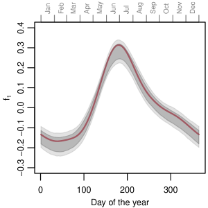
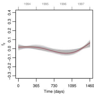
As we used a cyclic constraint for the seasonal effect, the ends of the function estimate meet, i.e., day 365 and day 1 are smoothly joined (see Figure 3). The effect showed a clear peak in the cool and dry winter months (May to August in the southern hemisphere) and a decreased risk of mortality in the warm summer months. This is in line with the results of other studies (e.g., Saldiva et al 1995). In the trend over the years (Figure 3), mortality decreased from 1994 to 1996 and increased thereafter. However, one should keep in mind that this trend needs to be combined with the periodical effect to form the complete temporal pattern.

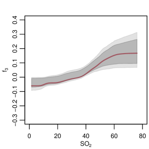
The estimated smooth effect for the pollutant SO₂ resulting from the model ‘mboost’ (Figure 3) indicated that an increase of the pollutant’s concentration does not result in a (substantially) higher mortality up to a concentration of $40\,\mu$g/m³. From this point onward, a steep increase in the expected mortality was observed, which flattened again for concentrations above $60\,\mu$g/m³. Hence, a dose-response relationship was observed, where higher pollutant concentrations result in a higher expected mortality. At the same time, the model indicated that increasing pollutant concentrations are almost harmless until a threshold is exceeded, and that the harm of SO₂ is not further increased after reaching an upper threshold. In an investigation of the effect of PM₁₀ Saldiva et al (1995) found no “safe” threshold in their study of elderly people in São Paulo. They also investigated the effect of SO₂ but did not report on details, such as possible threshold values, in this case. The more recent study on the effect of air pollution in São Paulo on children (Conceição et al 2001) used only linear effects for pollutant concentrations. Hence, no threshold values can be estimated.

The linear effects of the model ‘mboost’ (results not presented here; see R code in the electronic supplement) showed (small) negative effects of humidity and of minimum temperature (with a lag of 2 days), which indicates that higher humidity and higher minimum temperature reduce the expected number of deaths. Regarding the days of the week, mortality was higher on Monday than on Sunday and was even lower on all other days. This result might be due to different behavior and thus personal exposure to the pollutant on weekends or, more likely, due to a lag in recording on weekends.

(a)

(b)

Figure 4: Comparison of 4 the effect estimates for time (combination of long-term trend with the seasonal pattern) and 4 the effect estimates for SO₂. All effects are centered around zero.

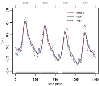
The resulting time trend of ‘mgcv’ is very similar compared to that of the model ‘mboost’ (Fig. 4), despite the fact that ‘mgcv’ was fitted without a cyclic constraint and thus allowing for a changing shape from year to year. However, the estimation of the complete time pattern without decomposition into the trend effect and the periodical, seasonal effect was less stable. The model ‘scam’ decomposes the seasonal pattern in the same manner as ‘mboost’ and uses a cyclic constraint for the day of the year and a smooth long term trend. Yet, the resulting effect estimate seems quite unstable at the boundary of the years where it shows some extra peaks. Modeling the trend and the periodic effect separately may have the disadvantage that some of the small-scale changes (e.g., around day 730) are missed. However, without this decomposition, models do not allow a direct inspection of the seasonal effect throughout the year. Hence, decomposing influence of time into seasonal effects and smooth long-term effects seems highly preferable as it offers a stable, yet flexible method to model the data and allows an easier and more profound interpretation.

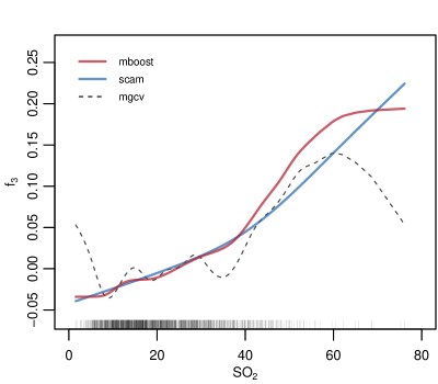
Both monotonic approaches (‘mboost’ and ‘scam’) showed a similar pattern in the effect of SO₂ (Fig. 4), but ‘scam’ does not flatten out for high values of the SO₂ concentration. Estimates from non-monotonic model (‘mgcv’) were very wiggly for small values up to a concentration of $40\,\mu$g/m³ and drop to zero for large values, which seems unreasonable.

Finally, all considered models had almost the same linear effects for the covariates (results not shown here; see R code in the electronic supplement). Hence, we can conclude that the linear effects in this model are very stable and are hardly influenced by the fitting method, i.e., boosting, penalized iteratively weighted least-squares (P-IWLS; see e.g., Wood 2008), or Newton-Raphson (Pya and Wood 2014), nor by constraints, i.e., monotonic or cyclic constraints, that are used to model the data.

Concerning the predictive accuracy, we compared the (negative) predictive log-likelihood of the two constrained models ‘mboost’ and ‘scam’ on 100 bootstrap samples. Both models performed almost identical with an average predictive risk of $1352.7$ (sd: $34.00$) for ‘mboost’ and of $1353.0$ (sd: $33.74$) for ‘scam’. Thus, in this low dimensional example boosting can well compete with standard approaches for constrained regression. In situations where variable selection is of major importance or when we want to fit models without assuming an exponential family, boosting shows its special strengths.

7.2 Activity of Roe Deer (Capreolus capreolus)

In the Bavarian Forest National Park (Germany), the applied wildlife management strategy is regularly examined. Part of the strategy involves trying to understand the activity profiles of the various species, including lynx, wild boar, and roe deer. The case study here focuses on the activity of European roe deer (Capreolus capreolus). According to Stache et al (2013), animal activity is influenced by exogenous factors, such as the azimuth of the sun (i.e., day/night rhythm and seasons), temperature, precipitation, and depth of snow. Another important role is played by endogenous factors, such as the species (e.g., reflected in their diet; roe deer are browsers), age, and sex. Additionally, as roe deer tend to be solitary animals, a high level of individual specific variation in activity is to be expected. The activity data was recorded using telemetry collars with an acceleration sensor unit. The activity is represented by a number ranging from 0 to 510, where higher values represent higher activity.

Activity profiles for the day and for the year were provided. As earlier analysis showed, the activity of males and females differs greatly. Hence, sex should be considered as an effect modifier in the analysis by defining sex-specific activity profiles. We considered a Gaussian model with the additive predictor

$$\begin{split}\mathds{E}(\text{activity}|\cdot)=\;&\mathbf{x}^{\top}\bm{\beta}+\text{temp}\cdot f_{1}(t_{\text{days}})\\ &+\text{depth of snow}\cdot f_{2}(t_{\text{days}})\\ &+\text{precipitation}\cdot f_{3}(t_{\text{days}})\\ &+f_{4}(t_{\text{hours}},t_{\text{days}})\\ &+I_{(\text{sex = male})}f_{5}(t_{\text{hours}},t_{\text{days}})+b_{\text{roe}},\end{split}$$

where $\mathbf{x}$ contains the categorical covariates sex, type of collar, year of observation, and age. Temperature, depth of snow, and precipitation entered the model rescaled to $|x|\leq 1$ by dividing the variables by the respective absolute maximum values. The effects of temperature ($f_{1}$), depth of snow ($f_{2}$), and precipitation ($f_{3}$) depend on the calendar day ($t_{\text{days}}$). An interaction surface ($f_{4}$) for time of the day ($t_{\text{hours}}$) and calendar day ($t$) was specified to flexibly model the daily activity profiles throughout the year. An additional effect for male roe deer was specified with $f_{5}$. Finally, a random intercept $b_{\text{roe}}$ for each roe deer was included. Details on the data set can be found in Online Resource 1 (Section LABEL:sec:roedeer_data), where we also describe the model specification in detail. R code is given as electronic supplement.

Results

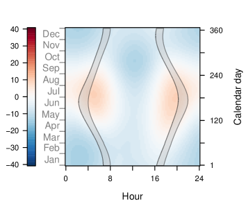
In the resulting model, six of ten base-learners were selected. The largest contribution to the model fit was given by the smooth interaction surfaces $f_{4}$ and $f_{5}$, which represent the time-dependent activity profiles for male and female roe deer (Figure 5). The individual activity of the roe deer $b_{\text{roe}}$ substantially contributed to the total predicted variation, with a range of approximately 20 units (not depicted here). The time-varying effects of temperature and depth of snow and the effect of the type of collar had a lower impact on the recorded activity of roe deer.

(a)

(b)

Figure 5: Influence of time on roe deer activity. Combined effect of calendar day and time of day 5 for female roe deer (= $f_{4}$) and 5 for male roe deer ($=f_{4}+f_{5}$), together with twilight phases (gray). White areas depict the mean activity level throughout the year; blue shading represents decreased activity, and red shading represents increased activity.

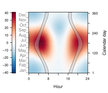
The activity profiles (Fig. 5) showed that roe deer were most active in and around the twilight phases in the mornings and evenings. This holds for the whole year and for both males and females. In general, the activity profiles of female and male roe deer were very similar, but male activity was much higher and had more variability. The activity of roe deer was strongly influenced by the season: During summer, the activity was much higher throughout the entire day. The phase of least activity was around noon. This behavior was enhanced in autumn. In spring, activity was more evenly distributed throughout the daytime, and lowest activity occurred during the hours after midnight.

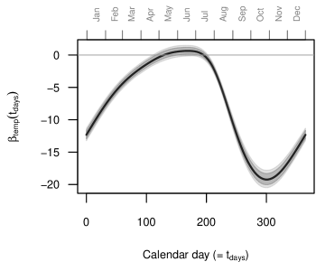
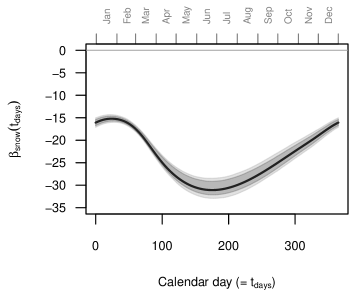
The effects of climatic variables are depicted in Figure 6. A higher temperature led to lower activity (negative effect of temperature), except from May to July, when higher temperatures led to higher activity (positive effect of temperature). The depth of snow had a negative effect on roe deer activity throughout the year, i.e., deeper snow led to lower activity. The effect of snow depth was stronger in the summer months (when there is hardly any snow), and less strong in January and February even though the snow depth was the greatest. Precipitation had no effect on roe deer activity according to our model.

(a)

(b)

Figure 6: Time-varying effects (i.e., $\beta(t_{\text{days}})$) of 6 temperature and 6 depth of snow together with 80% (dark gray) and 95% (light gray) point-wise bootstrap confidence intervals. Note that both variables are rescaled, i.e., $\beta(t_{\text{days}})$ is the maximal effect. On a given day, the effects of temperature and depth of snow are linear. The higher the amplitude for a given day, the stronger the effect will be.

7.3 Deer–vehicle Collisions in Bavaria

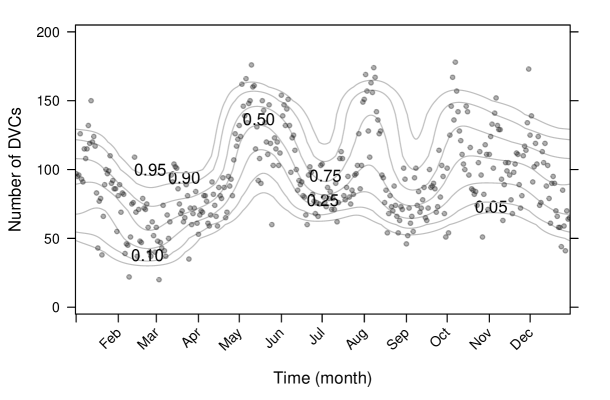
Important areas of application for both monotone and cyclic base-learners are conditional transformation models (Hothorn et al 2014b). Here, we describe the distribution of the number of deer–vehicle collisions (DVC) that took place throughout Bavaria, Germany, for each day $k=1,\dots,365$ of the year 2006 (see Hothorn et al 2012, for a more detailed description of the data), i.e.,

$$\mathbb{P}(\text{number of DVCs}\leq y|\text{day}=k)=\Phi(h(y|k)),$$

where $\Phi$ is the distribution function of the standard normal distribution. The conditional transformation function $h$ is parametrized as

$$h(y|k)=(\mathbf{B}_{\text{day}}(k)\otimes\mathbf{B}_{\text{DVC}}(y))\bm{\beta},$$

where $\mathbf{B}_{\text{day}}$ is a cyclic B-spline transformation for the day of the year (where Dec 31 and Jan 1 should match) and $\mathbf{B}_{\text{DVC}}$ is a B-spline transformation for the number of deer–vehicle collisions. The Kronecker product $\mathbf{B}_{\text{day}}(k)\otimes\mathbf{B}_{\text{DVC}}(y)$ defines a bivariate tensor product spline, which is fitted under smoothness constraints in both dimensions. Since the transformation function $h(y|k)$ must be monotone in $y$ for all days $k$ (otherwise $\Phi(h(y|k))$ is not a distribution function), a monotonicity constraint is needed for the second term, i.e., one requires monotonicity with respect to the number of deer–vehicle collisions but not with respect to time. The model was fitted by minimizing a scoring rule for probabilistic forecasts (e.g., Brier score or log score). Here, we applied the boosting approach described in (Hothorn et al 2014b). R code to fit the model is given as electronic supplement.

Results

We display the corresponding quantile functions over the course of the year 2006 in Figure 7. Three peaks (territorial movement at beginning of May, rut at end of July/ beginning of August, and early in October) were identified. While the first two peaks are expected, the significance of the third peak in October remains to be discussed with ecologists. Over the year, not only the mean but also higher moments of the distribution of the number of deer–vehicle collisions varied over time.

Figure 7: Number of deer–vehicle collisions (DVCs) in Bavaria, Germany, for each day of the year 2006. Superimposed lines depict the conditional quantiles ($5\%,10\%,25\%,50\%,75\%,90\%,95\%$) of this distribution for each day of the year.

8 Concluding Remarks

In this article, we extended the flexible modeling framework based on boosting to allow inclusion of monotonic or cyclic constraints for certain variables.

The monotonicity constraint on continuous variables leads to monotonic, yet smooth effects. Monotonic effects can be furthermore applied to bivariate P-splines. In this case, one can specify different monotonicity constraints for each variable separately. However, it is ensured that the resulting interaction surface is monotonic (as specified). Monotonicity constraints might be especially useful in, but are not necessarily restricted to, data sets with relatively few observations or noisy data. The introduction of monotonicity constraints can help to estimate more appropriate models that can be interpreted. In the context of conditional transformation models monotonicity constraints are an essential ingredient as we try to estimate distribution functions, which are per definition monotonic. Many other approaches to monotonic modeling result in non-smooth function estimates (e.g., Dette et al 2006, de Leeuw et al 2009, Fang and Meinshausen 2012). In the context of many applications, however, we feel that smooth effect estimates are more plausible and hence preferable.

Cyclic estimates can be easily used to model, for example, seasonal effects. The resulting estimate is a smooth effect estimate, where the boundaries are smoothly matched. Cyclic effects can be applied straightforwardly to model surfaces where the boundaries in each direction should match if cyclic tensor product P-splines are used. The idea of cyclic effects could also be extended to ordinal covariates with a temporal, periodic effect — such as days of the week.

Finally, both restrictions — monotonic and cyclic constraints — can be mixed in one model: Some of the covariates are monotonicity restricted, others have cyclic constraints and the rest is modeled, for example, as smooth effects without further restrictions or as linear effects.

Both monotonic P-splines and cyclic P-splines integrate seamlessly in the functional gradient descent boosting approach as implemented in mboost (Hofner et al 2014b, Hothorn et al 2014a). This allows a single framework for fitting possible complex models. Additionally, the idea of asymmetric penalties for adjacent coefficients can be transferred from P-splines to ordinal factors (Hofner et al 2011b), which can be integrated in the boosting framework as well. (Constrained) boosting approaches can be used in any situation where standard estimation techniques are used. They are especially useful, when variable and model selection are of major interest, and they can be used even if the number of variables is much larger than the number of observations ($p\gg n$). The proposed framework can be used to fit generalized additive models if one uses the negative log-likelihood as loss function. Other loss functions to fit constrained quantile or expectile regression models (Fenske et al 2011, Sobotka and Kneib 2012) or robust models with constraints based on the Huber loss can be used straight forward. The framework can be also transferred to conditional transformation models (Hothorn et al 2014b) or generalized additive models for location, scale and shape (GAMLSS; Rigby and Stasinopoulos 2005), where boosting methods where recently developed (Mayr et al 2012, Hofner et al 2014c).