Optimal Signal Recovery for Pulsed Balanced Detection

Abstract

We demonstrate a new tool for filtering technical and electronic noises from pulses of light, especially relevant for signal processing methods in quantum optics experiments as a means to achieve the shot-noise level and reduce strong technical noise by means of a pattern function. We provide the theory of this pattern-function filtering based on balance detection. Moreover, we implement an experimental demonstration where 10 dB of technical noise is filtered after balance detection. Such filter can readily be used for probing magnetic atomic ensembles in environments with strong technical noise.

I Introduction

Balanced detection provides a unique tool for many physical, biological and chemical applications. In particular, it has proven useful for improving the coherent detection in telecommunication systems Painchaud2009 ; Bach2005 , in the measurement of polarization squeezing Loudon1987 ; Banaszek1997 ; Zhang1998 ; Predojevic2008 ; Agha2010 , for the detection of polarization states of weak signals via homodyne detection Youn2005 ; Youn2012 , and in the study of light-atom interactions Kubasik2009 . Interestingly, balanced detection has proved to be useful when performing highly sensitive magnetometry Sheng2013 ; Budker2007 , even at the shot-noise level, in the continuous-wave Wolfgramm2010 ; Lucivero2014 and pulsed regimes Koschorreck2010 ; Behbood2013 .

The detection of light pulses at the shot-noise level with low or negligible noise contributions, namely from detection electronics (electronic noise) and from intensity fluctuations (technical noise), is of paramount importance in many quantum optics experiments. While electronic noise can be overcome by making use of better electronic equipment, technical noise requires special techniques to filter it, such as balanced detection and spectral filtering.

Even though several schemes have been implemented to overcome these noise sources Hansen2001 ; Chen2007 ; Windpassinger2009a , an optimal shot-noise signal recovery technique that can deal with both technical and electronic noises, has not been presented yet. In this paper, we provide a new tool based both on balanced detection and on the precise calculation of a specific pattern function that allows the optimal, shot-noise limited, signal recovery by digital filtering. To demonstrate its efficiency, we implement pattern-function filtering in the presence of strong technical and electronic noises. We demonstrate that up to 10 dB of technical noise for the highest average power of the beam, after balanced detection, can be removed from the signal. This is especially relevant in the measurement of polarization-rotation angles, where technical noise cannot be completely removed by means of balanced detectors Ruilova-Zavgorodniy2003 . Furthermore, we show that our scheme outperforms the Wiener filter, a widely used method in signal processing Vaseghi2000 .

The paper is organized as follows. In section II we present the theoretical model of the proposed technique, in section III we show the operation of this tool by designing and implementing an experiment, where high amount of noise (technical and electronic) is filtered. Finally in section IV we present the conclusions.

II Theoretical model

To optimally recover a pulsed signal in a balanced detection scheme, it is necessary to characterize the detector response, as well as the “electronic” and “technical” noise contributions Bachor2004 . We now introduce the theoretical framework of the filtering technique and show how optimal pulsed signal recovery can be achieved.

II.1 Model for a balanced detector

To model a balanced detector, see Fig. 1, we assume that it consists of 1) a polarizing beam splitter (PBS), which splits the $H$ and $V$ polarization components to two different detectors 2) the two detectors PD_H and PD_V, whose output currents are directly subtracted, and 3) a linear amplifier

Because the amplification is linear and stationary, we can describe the response of the detector by impulse response functions $h(\tau)$. If the photon flux at detector $X$ is $\phi_{X}(t)$, the electronic output can be defined as

$$v_{\rm out}(t)\equiv h_{H}*\phi_{H}+h_{V}*\phi_{V}+v_{N}(t),$$ (1)

where $v_{N}$ is the electronic noise of the photodiodes, including amplification. Here, $h*\phi$ stands for the convolution of $h$ and $\phi$, i.e., $(h*\phi)(t)\equiv\int_{-\infty}^{\infty}h(t-\tau)\phi(\tau)d\tau$. For clarity, the time dependence will be suppressed when possible. It is convenient to introduce the following notation: $\phi_{S}\equiv\phi_{H}+\phi_{V}$, $\phi_{D}\equiv\phi_{H}-\phi_{V}$, $h_{S}\equiv h_{H}+h_{V}$ and $h_{D}\equiv h_{H}-h_{V}$. Using these new variables, Eq. (1) takes the form

$$v_{\rm out}(t)=\frac{1}{2}\left({h}_{S}*{\phi}_{S}+{h}_{D}*{\phi}_{D}\right)+v_{N}(t).$$ (2)

From this signal, we are interested in recovering the differential photon number $S\equiv\int_{\mathcal{T}}\phi_{H}(t)dt-\int_{\mathcal{T}}\phi_{V}(t)dt$, where $\mathcal{T}$ is the time interval of the desired pulse, with minimal uncertainty. More precisely, we want to find an estimator $\hat{S}[v_{\rm out}(t)]$, that is unbiased $\langle\hat{S}\rangle=\langle{S}\rangle$, and has minimal variance ${\rm var\,}(\hat{S})$.

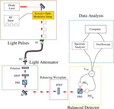
Figure 1: Scheme of the experimental setup. M, mirror, FC, fiber coupling, HWP, half-wave plate. See text for details.

II.2 Signal recovery estimator

In order to make $\hat{S}$ unbiased, we realize that it must linearly depend on $v_{\rm out}$. This because $S$ and $v_{\rm out}$ are linear in both $\phi_{H}$ and $\phi_{V}$. Therefore, the estimator must have the form

$$\hat{S}=\int_{-\infty}^{\infty}v_{\rm out}(t)\gamma(t)dt.$$ (3)

In Eq. (3), $\gamma(t)$ refers to as pattern function, which describes the most general linear estimator. In this work, we will consider three cases: 1) a raw estimator, $\gamma(t)=1$ for $t\in\mathcal{T}$ and 0 otherwise; 2) a Wiener estimator, which makes use of a Wiener-filter-like pattern function, $\gamma(t)=w(t)$, where $w(t)$ represents the Wiener filter in the time domain Vaseghi2000 , and 3) a model-based pattern function estimator $\gamma(t)=g(t)$. Notice that both $w(t)$ and $g(t)$ are defined in $(-\infty,\infty)$, allowing to properly choose a desired pulse. In what follows, we explicitly show how to calculate the model-based pattern function estimator $g(t)$.

II.3 Conditions of the pattern function

We assume that $\phi_{S},\phi_{D}$ have known averages (over many pulses) $\bar{\phi}_{S}(t),\bar{\phi}_{D}(t)$, and similarly the response functions $h_{S}(\tau),h_{D}(\tau)$ have averages $\bar{h}_{S}(\tau),\bar{h}_{D}(\tau)$. Then the average of the electronic output reads as

$$\bar{v}_{out}(t)=\frac{\overline{h}_{S}*\overline{\phi}_{S}+\overline{h}_{D}*\overline{\phi}_{D}}{2},$$ (4)

and $\langle\hat{S}\rangle=\int_{-\infty}^{\infty}dt\,g(t)\left(\bar{h}_{S}*\bar{\phi}_{S}+\bar{h}_{D}*\bar{\phi}_{D}\right)/2$. In writing Eq. (4), we have assumed that the noise sources are uncorrelated.

From this we observe that if a balanced optical signal is introduced, i.e. $\bar{\phi}_{D}=0$, the mean electronic signal $\bar{v}_{out}(t)$ is entirely due to $\overline{h}_{S}*\overline{\phi}_{S}$. In order that $\hat{S}$ correctly detects this null signal, $g(t)$ must be orthogonal to $\overline{h}_{S}*\overline{\phi}_{S}$, i.e.

$$\int_{-\infty}^{\infty}g(t)\cdot\left(\overline{h}_{S}*\overline{\phi}_{S}\right)(t)dt=0.$$ (5)

Our second condition derives from

$$\int_{-\infty}^{\infty}g(t)\cdot\left(\overline{h}_{D}*\overline{\phi}_{D}\right)(t)dt=\int_{\mathcal{T}}\overline{\phi}_{D}(t)dt,$$ (6)

which is in effect a calibration condition: the right-hand side is a uniform-weight integral of $\overline{\phi}_{D}$, while the left-hand side is a non-uniform-weight integral, giving preference to some parts of the signal. If the total weights are the same, the above gives $\langle\hat{S}\rangle=\langle S\rangle$. We note that this condition is not very restrictive. For example, given $\bar{h},\bar{\phi}$, and given $g(t)$ up to a normalization, the equation simply specifies the normalization of $g(t)$.

Notice that the condition given by Eq. (6) may still be somewhat ambiguous. If we want this to apply for all possible shapes $\bar{\phi}_{D}(t)$, it would imply $g(t)=$ const., and would make the whole exercise trivial. Instead, we make the physically reasonably assumption that the input pulse, with shape $\bar{\phi}_{S}$ is uniformly rotated to give $\bar{\phi}_{H}(t)$, $\bar{\phi}_{V}(t)\propto\bar{\phi}_{S}$. Similarly, it follows that $\bar{\phi}_{D}(t)\propto\bar{\phi}_{S}$. We note that this assumption is not strictly obeyed in our experiment and is a matter of mathematical convenience: a path difference from the PBS to the two detectors will introduce an arrival-time difference giving rise to opposite-polarity features at the start and end of the pulse, as seen in Fig. 3(a). A delay in the corresponding response functions $h$ is, however, equivalent, and we opt to absorb all path delays into the response functions. In our experiment the path difference is $\approx 5~{}\mathrm{cm}$, implying a time difference of less than 0.2 ns, much below the smallest features in Fig. 3(a). Absorbing the constant of proportionality into $g(t)$, we find

$$\int_{-\infty}^{\infty}g(t)\cdot\left(\overline{h}_{D}*\overline{\phi}_{S}\right)(t)dt=\int_{\mathcal{T}}\overline{\phi}_{S}(t)dt,$$ (7)

which is our calibration condition.

II.4 Noise model

We consider two kinds of technical noise: fluctuating detector response and fluctuating input pulses. We write the response functions in the form $h_{X}=\bar{h}_{X}+\delta h_{X}$, for a given detector $X$, where the fluctuating term $\delta h_{X}$ is a stochastic variable. Similarly, we write ${\phi}_{Y}=\bar{\phi}_{Y}+\delta\phi_{Y}$, where $Y$ is $H,V,S$ or $D$. By substituting the corresponding fluctuating response functions into Eq. (2), the electronic output signal becomes

$$v_{out}(t) = \frac{1}{2}\left(\overline{h}_{S}*\overline{\phi}_{S}+\overline{h}_{D}*\overline{\phi}_{D}\right)+v_{N}(t)$$ (8)

$$+\frac{1}{2}\left(\delta{h}_{S}*\overline{\phi}_{S}+\delta{h}_{D}*\overline{\phi}_{D}\right)$$

$$+\frac{1}{2}\left(\overline{h}_{S}*\delta{\phi}_{S}+\overline{h}_{D}*\delta{\phi}_{D}\right)+O(\delta h\,\delta\phi)$$

$$\approx \frac{1}{2}\left(\overline{h}_{S}*\overline{\phi}_{S}+\overline{h}_{D}*\overline{\phi}_{D}\right)+v_{N}(t)+v_{T}(t),$$ (9)

where $v_{T}(t)\equiv\frac{1}{2}(\delta{h}_{S}*\overline{\phi}_{S}+\delta{h}_{D}*\overline{\phi}_{D}+\overline{h}_{S}*\delta{\phi}_{S}+\overline{h}_{D}*\delta{\phi}_{D})$ is the summed technical noise from both $\delta h$ and $\delta\phi$ sources. We note that the optical technical noise, in contrast to optical quantum noise, scales as ${\rm var\,}(\delta\phi)\propto\bar{\phi}^{2}$, so that ${\rm var\,}(v_{T})\propto\bar{\phi}^{2}$. In passing to the last line we neglect terms $O(\delta h\,\delta\phi)$ on the assumption $\delta h\ll\bar{h}$, $\delta\phi\ll\bar{\phi}$. We further assume that $v_{N}$ and $v_{T}$ are uncorrelated.

We find the variance of the model-based estimator, $N_{\sigma}\equiv{\rm var\,}(\hat{S}_{\mathrm{opt}})$, is

$$N_{\sigma}=\left\langle\left|\int_{-\infty}^{\infty}g(t)v_{T}(t)dt\right|^{2}\right\rangle+\left<\left|\int_{-\infty}^{\infty}g(t)v_{N}(t)dt\right|^{2}\right>,$$ (10)

with the first term describing technical noise, and the second one electronic noise.

To compare against noise measurements, we transform Eq. (10) to the frequency domain. Using Parseval’s theorem, see Eq. (19), we can write the noise power as

$$\begin{split}N_{\sigma}=&\int_{-\infty}^{\infty}|G(\omega)|^{2}\langle|V_{T}(\omega)|^{2}+|V_{N}(\omega)|^{2}\rangle d\omega.\end{split}$$ (11)

Our goal is now to find the $G(\omega)$ that minimizes $N_{\sigma}$ satisfying the conditions in Eqs. (5) and (7), which in the frequency space are

$$I_{\rm or}\equiv\int_{-\infty}^{\infty}d\omega\,G^{*}(\omega)\overline{H}_{S}(\omega)\overline{\Phi}_{S}(\omega)=0,$$ (12)

$$I_{\rm cal}\equiv\int_{-\infty}^{\infty}d\omega\,G^{*}(\omega)\overline{H}_{D}(\omega)\overline{\Phi}_{S}(\omega)=\overline{\Phi}_{S}(0).$$ (13)

The specific form of the solution is given in Appendix B.

III Experiment

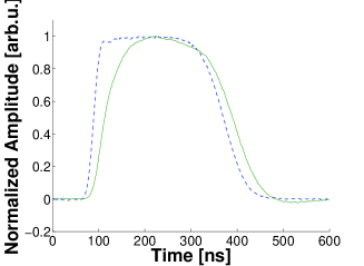
Figure 2: Average pulse shapes of the original pulse $p(t)$ at 150 MHz (blue dashed line) and the amplified one $p^{\prime}(t)$ at 5 MHz (green solid line). For the sake of comparison, both pulses are normalized.

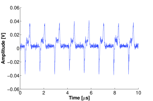
(a)

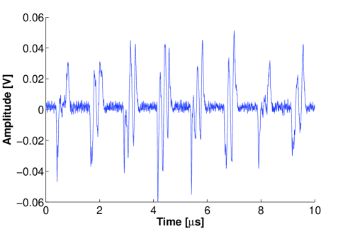
(b)

Figure 3: Example of pulses seen by the balanced detector (a) without technical noise, and (b) with technical noise introduced.

III.1 Pulse detection and detector characterization

In our experimental setup, pulsed signals are produced using an external cavity diode laser at 795 nm (Toptica DL100), modulated by two acousto-optic modulators (AOMs) in series. We have used two AOMs to prevent a shift in the optical frequency of the pulses, and also to ensure a high extinction ratio $(r_{e}>10^{7})$.

Balanced detection is performed by using a Thorlabs PDB150A detector Thorlabs2007 that contains two matched photodiodes wired back-to-back for direct current subtraction, amplified by a switchable-gain transimpedance amplifier. We use the gain settings $10^{3}$ V/A and $10^{5}$ V/A, with nominal bandwidths of 150 MHz and 5 MHz, respectively. Figure 2(a) shows the average pulse shapes $p(t)$ and $p^{\prime}(t)$, observed with bandwidth settings 150 MHz and 5 MHz, respectively. These shapes are obtained by blocking one detector and averaging over 1000 pulse traces (280 ns width).

In this way, to determine the impulse response functions $h_{H}(t)$, $h_{V}(t)$ of the photodiodes PD_H and PD_V, respectively, we first assume the form

$$h_{X}(t)=\frac{e^{-t/{\tau_{\mathrm{TIA}}}}-e^{-{t}/{\tau_{X}}}}{\tau_{\mathrm{TIA}}-\tau_{X}},$$ (14)

where $X\in\{H,V\}$ indicates the photodiode. This describes a single-pole filter with time constant $\tau_{X}$ for the photodiode Ezaki2006 ; Hamamatsu2012 followed by a single-pole filter with time-constant $\tau_{\mathrm{TIA}}$ for the transimpedance amplifier. We choose the parameters $\tau_{\mathrm{TIA}},\tau_{X}$ by a least-squares fit of

$$\tilde{p}^{\prime}(t)\equiv\int_{-\infty}^{\infty}p(\tau)h_{X}(t-\tau)d\tau.$$ (15)

to the measured traces $p^{\prime}(t)$ Saleh2007 .

As seen in Fig. 3(a), a small difference in the speeds of the two detectors leads to electronic pulses with a negative leading edge and a positive trailing edge, even when the optical signal is balanced, i.e. even when the average electronic output is zero.

III.2 Producing technical noise in a controlled manner

In order to prove that it is possible to remove technical noise, first we need to produce it in a controlled manner. To this end, we introduce technical noise in our system perturbing the main frequency of the AOMs using the circuit described in Fig. 4. The main frequency is produced by a voltage controlled oscillator (VCO) set to 80 MHz. Then, it is split with a power splitter, one of the arms is mixed with a signal from an arbitrary wave generator (AWG) and attenuated, whereas in the other arm the signal is passed by a phase shifter. Finally, both signals are put back together with a power combiner. In this way, we have a main frequency of 80 MHz and sidebands at the frequency of the signal introduced with the AWG. We can then program the AWG with technical noise for a particular frequency and bandwidth, as illustrated in Fig. 5.

Figure 4: Scheme of the electronic circuit used to introduce technical noise into the AOMs. See text for details.

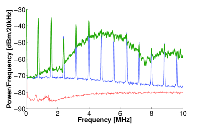
Figure 5: Illustration of noise contributions in the power spectrum of a train of pulses. Thin red curve shows the electronic noise of the detector, i.e., with no optical signal introduced. Blue medium curve shows power spectrum with no introduced technical noise. This shows narrow peaks at harmonics of the pulse repetition frequency rising from a shot-noise background. The roll-off in signal strength is due to the 5 MHz bandwidth of the detector. Thick green curve shows power spectrum with an introduced technical noise with central frequency of 5 MHz and FWHM bandwidth of 1 MHz.

In our setup, we have fixed the parameters of the circuit and the AWG for generating about 10 dB of technical noise for an optical power of $400~{}\mu W$ with a duty cycle of the pulses of $1/3$.

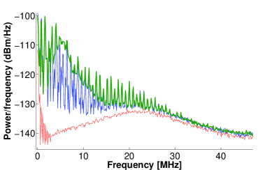
Figure 6: Power spectral density from a train of 800 pulses, considering three cases: signal without technical noise (blue line), signal with technical noise (bold green line), and electronic noise (red thin line).

III.3 Calculating the optimal pattern function for different optical powers

To measure the noise spectra upon which the pattern function will be based, we use an oscilloscope (Lecroy Wavejet-324), rather than a spectrum analyzer. This allows us to use the same instrument for noise characterization and optimization as we will later use to acquire signals to process by digital filtering.

We collect $5\times 10^{5}$ samples in a 1000 $\mu\text{s}$ acquisition time containing a total of 800 pulses $\sim$400 ns duration, with a duty cycle of 1/3. For this train of pulses we compute the power spectral density (PSD) for three cases: 1) signal without added technical noise, 2) signal with added technical noise, and 3) the electronic noise. Figure 6 shows an example of PSD calculated for these cases. From these PSDs we can then extract the parameters necessary for computing the optimal pattern function, namely electronic background, technical noise power and shot-noise power. Using these parameters, and following the method explained in section II, we have calculated the optimal pattern function $g(t)$ for different average powers of the beam, from 0 to 400 $\mu$W in steps of 20 $\mu$W.

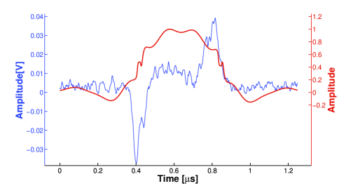
Figure 7: Example of cutting of the pulses (blue thin line) and the corresponding pattern function (red thick line).

III.4 Shot-noise limited detection with pulses and measurement of the technical noise with pulses

Because the pulses are non-overlapping, as seen in Fig. 3, we can isolate any single pulse by keeping only the signal in a finite window containing the pulse, to get a waveform as illustrated in Fig. 7. Also shown there is the optimal pattern function. This illustrates some qualitative features of the optimal pattern function, which is 1) orthogonal to the residual common-mode signal $h_{S}*\phi_{S}$, which first goes negative and then positive, 2) well overlapped with the differential-mode signal $h_{D}*\phi_{D}$, which is positive, and 3) smooth with some ringing, to suppress both high-frequency and low-frequency noise.

For each pulse we compute the estimators $\hat{S}_{\rm raw}$, $\hat{S}_{\rm W}$ and $\hat{S}_{\rm opt}$, using pattern functions $\gamma(t)=1$ (raw estimator), $\gamma(t)=w(t)$ (Wiener estimator) and $\gamma(t)=g(t)$ (optimal model-based estimator), respectively. The Wiener filter $w(t)$ can be defined as the Fourier transform of the frequency domain representation of the Wiener filter $W(\omega)$, given by the ratio of the cross-power spectrum of the noisy signal with the desired signal over the power spectrum of the noisy signal Vaseghi2000 . For more details see the appendix C.

III.4.1 Shot-noise limited detection with pulses

We first show that the system is shot-noise limited in the absence of added technical noise. For this, we compute the variance of $\hat{S}_{\rm raw}$, this variance is a noise estimation, computed from a pulse train without technical noise, as a function of optical power $P$. We fit the resulting variances with the quadratic ${\rm var\,}(\hat{S}_{\rm raw})=A+BP+CP^{2}$, and obtain $A=4.5\pm 0.3\times 10^{-20}J^{2}$, $B=2.4\pm 0.1\times 10^{-22}J^{2}/\mu W$ and $C=6.7\pm 0.6\times 10^{-26}J^{2}/\mu W^{2}$. The data and fit are shown in Fig. 8(a), and clearly show a linear dependence on $P$, a hallmark of shot-noise limited performance.

III.4.2 Measuring technical noise with pulses

Now, we proceed as before with the exception that in this case we introduce technical noise to the signal. We obtain the following fitting parameters: $A=4.5\pm 0.3\times 10^{-20}J^{2}$, $B=1.9\pm 0.1\times 10^{-22}J^{2}/\mu W$ and $C=4.12\pm 0.05\times 10^{-24}J^{2}/\mu W^{2}$.

We observe from Fig. 8(b) that the noise estimation for the data that has technical noise exhibits a clearly quadratic trend, in contrast to the linear behavior where no technical noise is introduced. The results shown in Figs. 8(a) and 8(b) prove that, with our designed system, it is possible to introduce technical noise in a controlled way.

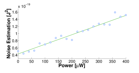
(a)

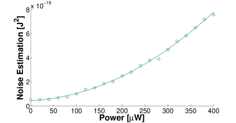
(b)

Figure 8: Computed noise estimation as a function of the optical signal power (a) without and (b) with technical noise introduced. Circles: experimental data, solid line: quadratic fit.

III.5 Filtering 10 dB of technical noise using an optimal pattern function

To illustrate the performance of our technique when filtering technical noise, we introduce a high amount of noise —about $60$ dB above the shot noise level at the maximum optical power— to the light pulses produced by the AOMs. After balancing a maximum of 10 dB remains in the electronic output, which is then filtered by means of the optimal pattern function technique.

We have verified the correct noise filtering by comparing the results with shot-noise limited pulses. For this purpose, we compute ${\rm var\,}(\hat{S}_{\rm opt})$, the variance of the optimal estimator for each power, and for each data set, the shot-noise limited and the noisy one. Figure 9 shows the computed noise estimation as function of the optical power for both. Notice that the two noise estimations are linear with the optical power. Moreover, we observe that both curves agree at $\sim 91\pm 5\%$, using the ratio of the slopes, which allows us to conclude that, by using this technique, we can retrieve shot-noise limited pulses from signals bearing high amount of technical noise.

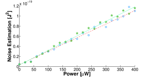
Figure 9: Computed noise estimation using the optimal pattern estimator as a function of the optical power for shot-noise limited pulses (blue circles) and pulses with technical noise (green stars). Their corresponding quadratic fits are shown in red dashed and cyan lines, respectively.

III.6 Optimal estimation of the polarization-rotation angle.

The experimental setup that we have implemented, see Fig. 1, can perform also as a pulsed signal polarimeter. For instance, it is possible to determine a small polarization-rotation angle $\varphi$ from a $45^{\circ}$ linear polarized light pulse. Along these lines, we make use of three estimators $\hat{S}_{\rm raw},\hat{S}_{\rm W}$ and $\hat{S}_{\rm opt}$ to determine the amount of noise on the estimation of the polarization-rotation angle. From the obtained results, we show that the model-based estimator outperforms the other two.

We proceed to calculate the noise on the polarization-rotation angle $\varphi$ estimation, for this determination we calculate the variance of $\varphi$. We notice that the Taylor approximation of the variance of $\hat{S}(\varphi)$ is

$${\rm var\,}(\hat{S})\approx\left(\frac{d\hat{S}}{d\varphi}\right)^{2}{\rm var\,}(\varphi).$$ (16)

For small angles $\varphi$, the function $\hat{S}(\varphi)$ is approximately linear on $\varphi$, so the contribution from higher order terms can be disregarded.

Therefore, the noise on the angle estimation is

$${\rm var\,}(\varphi)=\frac{{\rm var\,}(\hat{S})}{\left(\frac{d{\hat{S}}}{d\varphi}\right)^{2}}.$$ (17)

We can then compute this expression using the three before mentioned estimators. For such task we use the experimental data together with an analytical approximation of the derivative, that takes as input the measured data. Figure 10 depicts the noise angle estimation, showing that the optimal pattern function performs better than the other estimators when eliminating the technical noise and reducing the electronic noise. In particular, the based-model estimator surpasses the Wiener estimator, which is a widely used method in signal processing Vaseghi2000 .

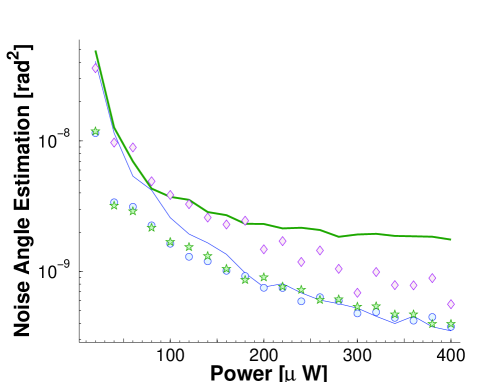
Figure 10: Noise angle estimation as a function on the optical power. Raw estimators with technical noise (green bold line) and without (blue medium line). Wiener estimator with technical noise (pink diamonds). Model-based estimators with technical noise (green stars) and without (blue circles). For the sake of visualization the results are presented in a semi-log graph.

IV Conclusions

We have studied in theory and with an experimental demonstration, the optimal recovery of light pulses via balanced detection. We developed a theoretical model for a balanced detector and the noise related to the detection of optical pulses. We minimized the technical and electronic noise contributions obtaining the optimal (model-based) pattern function. We designed and implemented an experimental setup to test the introduced theoretical model. In this experimental setup, we produced technical noise in a controlled way, and retrieved shot-noise limited signals from signals bearing about 10 dB of technical noise after balanced detection. Finally, we compare against naïve and Wiener filter estimation for measuring rotation angles, and confirm superior performance of the model-based estimator.

The results presented here might lead to a better polarization-rotation angle estimations when using pulses leading to probe magnetic atomic ensembles in environments with technical noise Koschorreck2010 ; SewellPRL2012 . This possibility is especially attractive for balanced detection of sub-shot-noise pulses Predojevic2008 ; Wolfgramm2010 , for which the acceptable noise levels are still lower.

Appendix A Parseval

We note the inner-product form of Parseval’s theorem

$$\int_{-\infty}^{\infty}G^{*}(t)x(t)dt=\int_{-\infty}^{\infty}G^{*}(\omega)X(\omega)d\omega,$$ (18)

where the functions $G(\omega),X(\omega)$ are the Fourier transforms of $g(t),x(t)$, respectively. For any stationary random variable $x(t)$, $\langle X(\omega)X(\omega^{\prime})\rangle=\delta(\omega-\omega^{\prime})$ (if this were not the case, there would be a phase relation between different frequency components, which contradicts the assumption of stationarity). From this, it follows that

$$\left\langle\left|\int_{-\infty}^{\infty}g(t)x(t)dt\right|^{2}\right\rangle=\int_{-\infty}^{\infty}|G(\omega)|^{2}\langle|X(\omega)|^{2}\rangle d\omega.$$ (19)

Appendix B Formal derivation of the pattern function

We will minimize the noise power $N_{\sigma}$ (see Eq. (11)) with respect to the pattern function $G(\omega)$ using the two conditions (see Eq. (12) and Eq. (13)). We solve this by the method of Lagrange multipliers. For this, we write

$$L(G,\lambda_{1},\lambda_{2})=N_{\sigma}+\lambda_{1}(I_{\rm or}-0)+\lambda_{2}(I_{\rm cal}-\overline{\Phi}_{S}({\omega=0})),$$ (20)

and then solve the equations

$$\partial_{G^{*}}L = 0,$$

$$\partial_{\lambda_{1}}L = 0,$$

$$\partial_{\lambda_{2}}L = 0.$$ (21)

The first equation reads

$$\partial_{G^{*}}L = G(\omega)\langle|V_{T}(\omega)|^{2}+|V_{N}(\omega)|^{2}\rangle$$

$$+\lambda_{1}\overline{H}_{S}(\omega)\overline{\Phi}_{S}(\omega)+\lambda_{2}\overline{H}_{D}(\omega)\overline{\Phi}_{D}(\omega)=0,$$

with formal solution

$$G(\omega)=\frac{\lambda_{1}\overline{H}_{S}(\omega)\overline{\Phi}_{S}(\omega)+\lambda_{2}\overline{H}_{D}(\omega)\overline{\Phi}_{D}(\omega)}{\langle|V_{T}(\omega)|^{2}\rangle+\langle|V_{N}(\omega)|^{2}\rangle}.$$ (23)

The second and third equations from Eq. (B) are the same as Eq. (12) and Eq. (13) above. The problem is then reduced to finding $\lambda_{1}$, $\lambda_{2}$ which (through the above), make $G(\omega)$ satisfy the two constraints.

Substituting Eq. (23) into Eq. (12) and Eq. (13), we find

$$O_{1}\lambda_{1}+O_{2}\lambda_{2}=0,$$ (24)

and

$$C_{1}\lambda_{1}+C_{2}\lambda_{2}=\Phi_{0}.$$ (25)

where

$$O_{1}\equiv\int_{-\infty}^{\infty}\frac{|\overline{H}_{S}(\omega)|^{2}|\overline{\Phi}_{S}(\omega)|^{2}}{\langle|V_{T}(\omega)|^{2}\rangle+\langle|V_{N}(\omega)|^{2}\rangle}d\omega,$$ (26)

$$O_{2}\equiv\int_{-\infty}^{\infty}\frac{\overline{H}^{*}_{D}(\omega)\overline{\Phi}^{*}_{S}(\omega)\cdot\overline{H}_{S}(\omega)\overline{\Phi}_{S}(\omega)}{\langle|V_{T}(\omega)|^{2}\rangle+\langle|V_{N}(\omega)|^{2}\rangle}d\omega,$$ (27)

$$C_{1}\equiv\int_{-\infty}^{\infty}\frac{\overline{H}^{*}_{S}(\omega)\overline{\Phi}^{*}_{S}(\omega)\cdot\overline{H}_{D}(\omega)\overline{\Phi}_{S}(\omega)}{\langle|V_{T}(\omega)|^{2}\rangle+\langle|V_{N}(\omega)|^{2}\rangle}d\omega,$$ (28)

$$C_{2}\equiv\int_{-\infty}^{\infty}\frac{|\overline{H}_{D}(\omega)|^{2}|\overline{\Phi}_{S}(\omega)|^{2}}{\langle|V_{T}(\omega)|^{2}\rangle+\langle|V_{N}(\omega)|^{2}\rangle}d\omega,$$ (29)

with $\Phi_{0}\equiv\overline{\Phi}_{S}({\omega=0})$. The solution to the set of Eqs. (24) and (25) is then given by

$$\lambda_{1}=\frac{\Phi_{0}O_{2}}{C_{1}O_{2}-C_{2}O_{1}},\quad\lambda_{2}=\frac{\Phi_{0}O_{1}}{C_{2}O_{1}-C_{1}O_{2}}.$$ (30)

It should be noted that quantum noise is not explicitly considered in the model. Rather, it is implicitly present in $\phi_{H},\phi_{V}$ which may differ from their average values $\bar{\phi}_{H},\bar{\phi}_{V}$ due to quantum noise. Note that the point of this measurement design is to optimize the measurement of $\int_{\mathcal{T}}\phi_{H}(t)-\phi_{V}(t)dt,$ including the quantum noise in that variable. For this reason, it is sufficient to describe, and minimize, the other contributions.

Appendix C Wiener filter estimator

The Wiener filter estimator $\hat{S}_{\rm W}$ can be derived from the frequency domain Wiener filter output $\hat{X}(\omega)$ Vaseghi2000 define as

$$\hat{X}(\omega)\equiv W(\omega)V(\omega),$$ (31)

where $W(\omega)$ and $V(\omega)$ are the Wiener filter and the electronic output in frequency domain, respectively.

We define $W^{\prime}(\omega)\equiv W^{*}(\omega)$ and $w^{\prime}(t)\equiv w^{*}(t)$ and make use of the inner product of the Parseval’s theorem, see Eq. (18).

$$\int_{-\infty}^{\infty}W^{\prime}(\omega)V_{\mathrm{out}}(\omega)d\omega=\int_{-\infty}^{\infty}w^{\prime}(t)v_{\mathrm{out}}(t)dt.$$ (32)

Then the Wiener filter estimator $\hat{S}_{\rm W}$ is $\int_{-\infty}^{\infty}w^{\prime}(t)v_{\mathrm{out}}(t)dt$ corresponding to Eq. (3) for $\gamma(t)=w^{\prime}(t)$.

The Wiener filter $W(\omega)$ is

$$W(\omega)=\frac{\langle|V_{\mathrm{ideal}}^{*}(\omega)V_{\mathrm{out}}(\omega)|\rangle}{\langle|V_{\mathrm{out}}(\omega)|^{2}\rangle}.$$ (33)

In order to compute the Wiener filter it is necessary to construct the ideal signal $V_{\mathrm{ideal}}(\omega)$, a signal without all noise contributions.

- (1) Y. Painchaud, M. Poulin, M. Morin, and M. Tétu, “Performance of balanced detectionin a coherent receiver,” Opt. Express 17, 3659–3672 (2009).
- (2) H.-G. Bach, “Ultra-broadband photodiodes and balanced detectors towards 100 gbit/s and beyond,” in “Optics East 2005,” (International Society for Optics and Photonics, 2005), pp. 60,140B–60,140B–13.
- (3) R. Loudon and P. Knight, “Squeezed light,” Journal of Modern Optics 34, 709–759 (1987).
- (4) K. Banaszek and K. Wódkiewicz, “Operational theory of homodyne detection,” Phys. Rev. A 55, 3117–3123 (1997).
- (5) T. C. Zhang, J. X. Zhang, C. D. Xie, and K. C. Peng, “How does an imperfect system affect the measurement of squeezing?” Acta Physica Sinica-overseas Edition 7, 340–347 (1998).
- (6) A. Predojević, Z. Zhai, J. M. Caballero, and M. W. Mitchell, “Rubidium resonant squeezed light from a diode-pumped optical-parametric oscillator,” Phys. Rev. A 78, 063,820– (2008).
- (7) I. H. Agha, G. Messin, and P. Grangier, “Generation of pulsed and continuous-wave squeezed light with rb-87 vapor,” Optics Express 18, 4198–4205 (2010).
- (8) S.-H. Youn, “Novel scheme of polarization-modulated ordinary homodyne detection for measuring the polarization state of a weak field,” Journal of the Korean Physical Society 47, 803–808 (2005).
- (9) S.-H. Youn, Measurement of the Polarization State of a Weak Signal Field by Homodyne Detection (InTech, available from: http://www.intechopen.com/books/photodetectors/, from the book Gateva2012 , 2012), chap. 17, pp. 389–404.
- (10) M. Kubasik, M. Koschorreck, M. Napolitano, S. R. de Echaniz, H. Crepaz, J. Eschner, E. S. Polzik, and M. W. Mitchell, “Polarization-based light-atom quantum interface with an all-optical trap,” Phys. Rev. A 79, 043,815– (2009).
- (11) D. Sheng, S. Li, N. Dural, and M. V. Romalis, “Subfemtotesla scalar atomic magnetometry using multipass cells,” Phys. Rev. Lett. 110, 160,802– (2013).
- (12) D. Budker and M. Romalis, “Optical magnetometry,” Nature Physics 3, 227–234 (2007).
- (13) F. Wolfgramm, A. Cerè;, F. A. Beduini, A. Predojević, M. Koschorreck, and M. W. Mitchell, “Squeezed-light optical magnetometry,” Phys. Rev. Lett. 105, 053,601– (2010).
- (14) V. G. Lucivero, P. Anielski, W. Gawlik, and M. W. Mitchell, “Shot-noise-limited magnetometer with sub-pt sensitivity at room temperature,” arXiv quant-ph, 1403.7796 (submitted to Phys. Rev. A) (2014).
- (15) M. Koschorreck, M. Napolitano, B. Dubost, and M. W. Mitchell, “Sub-projection-noise sensitivity in broadband atomic magnetometry,” Phys. Rev. Lett. 104, 093,602– (2010).
- (16) N. Behbood, F. M. Ciurana, G. Colangelo, M. Napolitano, M. W. Mitchell, and R. J. Sewell, “Real-time vector field tracking with a cold-atom magnetometer,” Applied physics letters 102, 173,504– (2013).
- (17) H. Hansen, T. Aichele, C. Hettich, P. Lodahl, A. I. Lvovsky, J. Mlynek, and S. Schiller, “Ultrasensitive pulsed, balanced homodyne detector: application to time-domain quantum measurements,” Opt. Lett. 26, 1714–1716 (2001).
- (18) Y. Chen, D. M. de Bruin, C. Kerbage, and J. F. de Boer, “Spectrally balanced detection for optical frequency domain imaging,” Opt. Express 15, 16,390–16,399 (2007).
- (19) P. J. Windpassinger, M. Kubasik, M. Koschorreck, A. Boisen, N. Kjærgaard, E. S. Polzik, and J. H. Müller, “Ultra low-noise differential ac-coupled photodetector for sensitive pulse detection applications,” Measurement Science and Technology 20, 055,301 (2009).
- (20) V. Ruilova-Zavgorodniy, D. Y. Parashchuk, and I. Gvozdkova, “Highly sensitive pump–probe polarimetry: Measurements of polarization rotation, ellipticity, and depolarization,” Instruments and Experimental Techniques 46, 818–823 (2003).
- (21) S. V. Vaseghi, Advanced Digital Signal Processing and Noise Reduction (John Wiley & Sons Ltd, 2000).
- (22) H.-A. Bachor and T. C. Ralph, A Guide to Experiments in Quantum Optics (Wiley-VCH, 2004).
- (23) Thorlabs, Operation Manual Thorlabs Instrumentation PDB100 Series Balanced Amplified Photodetectors PDB150 (2007).
- (24) T. Ezaki, G. Suzuki, K. Konno, O. Matsushima, Y. Mizukane, D. Navarro, M. Miyake, N. Sadachika, H.-J. Mattausch, and M. Miura-Mattausch, “Physics-based photodiode model enabling consistent opto-electronic circuit simulation,” in “Electron Devices Meeting, 2006. IEDM ’06. International,” (2006), pp. 1–4.
- (25) K. K. Hamamatsu Photonics, Opto-semiconductor handbook — Chapter 2: Si photodiodes (Hamamatsu, available from: https://www.hamamatsu.com/sp/ssd/doc_en.html, 2012), chap. 2, pp. 22–66.
- (26) B. E. A. Saleh and M. C. Teich, Fundamentals of Photonics (Wiley, 2007).
- (27) R. J. Sewell, M. Koschorreck, M. Napolitano, B. Dubost, N. Behbood, and M. W. Mitchell, “Magnetic sensitivity beyond the projection noise limit by spin squeezing,” Phys. Rev. Lett. 109, 253,605 (2012).
- (28) S. Gateva, ed., Photodetectors (InTech, available from: http://www.intechopen.com/books/photodetectors/, 2012).