A near infrared test for two recent luminosity functions for galaxies

Este documento describe ..

Abstract

Two recent luminosity function (LF) for galaxies are reviewed and the parameters which characterize the near infrared are fixed. A first LF is a modified Schechter LF with four parameters. The second LF is derived from the generalized gamma and has four parameters. The formulas which give the number of galaxies as function of the redshift are reviewed and a special attention is given to the position of the photometric maximum which is expressed as function of a critical parameter or the flux of radiation or the apparent magnitude. A simulation of the 2MASS Redshift Survey is given in the framework of the non Poissonian Voronoi Tessellation.

Galaxies: luminosity function Statistical distributions Galaxies Clusters of galaxies

0.1 Introduction

The release of the 2MASS Redshift Survey (2MRS), with it’s 44599 galaxies having $K_{s}<11.75$ allows to make tests on the radial number of galaxies because we have a small zone-of-avoidance , see Figure 1 in Huchra et al. (2012). The number of galaxies as function of the redshift , $z$, is strictly related to the chosen luminosity function for galaxies (LF). The most used LF is the Schechter function , introduced by Schechter (1976) , but also two recent LFs, the generalized gamma with four parameters, see Zaninetti (2010), and the modified Schechter LF , see Alcaniz & Lima (2004), can model the LF for galaxies. We now outline some topic issues in which the LF plays a relevant role : determination of the parameters at different $z$ , see Goto et al. (2011), evaluation of the parameters taking account of the star formation (SF) and presence of active nuclei, see Wu et al. (2011), determination of the normalization in the Near Infrared (NIR) as function of $z$, see Keenan et al. (2012).

In this paper Section 0.2 first reviews two recent LFs for galaxies and then derives the free parameters in the near infrared band. Once the basic parameters of the recent LFs are derived we make a comparison between observed radial distribution in the number of galaxies and theoretical predictions, see Section 0.3. A simulation of the near infrared all sky survey is reported in Section 0.4.

0.2 The luminosity functions

This Section reviews the standard luminosity function (LF) for galaxies, and two recent LF for galaxies. A first test is done on Table 2 of Cole et al. (2001) where the combined data of the Two Micron All Sky Survey (2MASS) Extended Source Catalog and the 2dF Galaxy Redshift Survey allowed to build a luminosity function in the $K_{s}$ band (2MASS Kron magnitudes). The main statistical test is done through the $\chi^{2}$,

$$\chi^{2}=\sum_{i=1}^{n}\frac{(T_{i}-O_{i})^{2}}{T_{i}},$$ (1)

where $n$ is the number of bins, $T_{i}$ is the theoretical value, and $O_{i}$ is the experimental value represented by the frequencies. A reduced merit function $\chi_{red}^{2}$ is evaluated by

$$\chi_{red}^{2}=\chi^{2}/NF\quad,$$ (2)

where $NF=n-k$ is the number of degrees of freedom, $n$ is the number of bins, and $k$ is the number of parameters.

0.2.1 The Schechter function

The Schechter function, introduced by Schechter (1976), provides a useful fit for the LF of galaxies

$$\Phi(L)dL=(\frac{\Phi^{*}}{L^{*}})(\frac{L}{L^{*}})^{\alpha}\exp\bigl{(}{-\frac{L}{L^{*}}}\bigr{)}dL\quad,$$ (3)

here $\alpha$ sets the slope for low values of $L$ , $L^{*}$ is the characteristic luminosity and $\Phi^{*}$ is the normalization. The equivalent distribution in absolute magnitude is

$$\Phi(M)dM=0.921\Phi^{*}10^{0.4(\alpha+1)(M^{*}-M)}\exp\bigl{(}{-10^{0.4(M^{*}-M)}}\bigr{)}dM\,,$$ (4)

where $M^{*}$ is the characteristic magnitude as derived from the data. The scaling with $h$ is $M^{*}-5\log_{10}h$ and $\Phi^{*}\leavevmode\nobreak\ h^{3}\leavevmode\nobreak\ [Mpc^{-3}]$.

0.2.2 A modified Schechter function

In order to improve the flexibility at the bright end Alcaniz & Lima (2004) introduced a new parameter $\eta$ in the Schechter LF

$$\Phi(L)dL=\frac{{\it\Phi^{*}}\,\left({\frac{L}{{\it L^{*}}}}\right)^{\alpha}\left(1-{\frac{\left(\eta-1\right)L}{{\it L^{*}}}}\right)^{\frac{1}{\eta-1}}}{{\it L^{*}}}dL\quad.$$ (5)

This new LF in the case of $\eta<1$ is defined in the range $0<L<L_{max}$ where $L_{max}=\frac{L^{*}}{\eta-1}$ and therefore has a natural upper boundary which is not infinity. In the limit $\lim_{\eta\to 1}\Phi(L)$ the Schechter LF is obtained. In the case of $\eta>1$ the average value is

$${\langle L\rangle}=\frac{{\it\Phi^{*}}{\it L^{*}}\,\Gamma\left(3+\alpha\right)\Gamma\left(1+\left(\eta-1\right)^{-1}\right)\left(\eta-1\right)^{-\alpha-2}}{\Gamma\left(3+\alpha+\left(\eta-1\right)^{-1}\right)\left(\alpha+2\right)}\quad,$$ (6)

and in the case of $\eta<1$ the average value is

$${\langle L\rangle}=\frac{{\it\Phi^{*}}{\it L^{*}}\,\left(-\eta+1\right)^{-2-\alpha}\,\Gamma\left(-{\frac{-1+2\,\eta+\alpha\,\eta-\alpha}{\eta-1}}\right)\Gamma\left(2+\alpha\right)}{\Gamma\left(-\left(\eta-1\right)^{-1}\right)}\quad.$$ (7)

The distribution in magnitude is :

$$\Phi(M)dM=0.921\Phi^{*}10^{0.4(M^{*}-M)(\alpha+1)}(1-(\eta-1)10^{0.4(M^{*}-M)})^{\frac{1}{\eta-1}}dM\quad.$$ (8)

Table 1 reports the parameters of the Schechter and the modified Schechter LF applied to the $K_{s}$ band.

Table 1: Numerical values values and $\chi^{2}_{red}$ of the three LFs applied to $K_{S}$ band (2MASS Kron magnitudes) with data as extracted from Table 2 in Cole et al. 2001 when $M_{\sun}$=3.39  .

LF	parameters	$\chi^{2}_{red}$
Schechter, Coles 2001	$M^{*}$= -23.77, $\alpha$=-1.14,
	$\Phi^{*}=0.0114/Mpc^{3}$
Schechter, our code	$M^{*}$= -23.289, $\alpha$=-0.794,	1.38
	$\Phi^{*}=0.0128/Mpc^{3}$
Modified Schechter	$M^{*}$= -23.119, $\alpha$= -0.707,	1.36
	$\Phi^{*}=0.0142/Mpc^{3}$ , $\eta=0.956$
Generalized gamma	$M^{*}$= -23.14 , k=0.946,c=0.28	1.42
	$\Psi^{*}=0.0481/Mpc^{3}$

The Schechter LF, the modified Schechter LF as well the observed data in the $K_{S}$ band are reported in Figure 1.

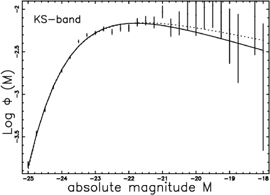
Figure 1: The luminosity function data of the $K_{S}$ band are represented with error bars. The continuous line fit represents the modified Schechter LF (eqn. 8) and the dotted line represents the Schechter LF (eqn.4).

0.2.3 The generalized gamma distribution with four parameters

A four parameter generalized gamma LF has been derived in Zaninetti (2010)

$$\Psi(L;L^{*},c,k,\Psi^{*})=\Psi^{*}\frac{{\it k}\,\left({\frac{L}{L^{*}}}\right)^{c{\it k}-1}{{\rm e}^{-\left({\frac{L}{L^{*}}}\right)^{{\it k}}}}}{L^{*}\Gamma\left(c\right)}\quad.$$ (9)

This function contains the four parameters $c$, $k$, $L^{*}$ and $\Psi^{*}$ and the range of existence is $0\leq L<\infty$. The averaged luminosity is

$${\langle L\rangle}=\frac{{\it L^{*}}\,\Gamma\left({\frac{1+ck}{k}}\right)}{\Gamma\left(c\right)}\quad.$$ (10)

The magnitude version of this LF is

$$\Psi(M)dM=\frac{{\Psi^{*}}0.4\ln\left(10\right)k{10}^{-0.4ck\left(M-{M^{*}}\right)}{{\rm e}^{-{10}^{-0.4\left(M-{M^{*}}\right)k}}}}{\Gamma\left(c\right)}\\ dM\,.$$

The Schechter LF, the generalized gamma LF as well the observed data in the $K_{S}$ band are reported in Figure 2 and the adopted parameters in Table 1.

Figure 2: The luminosity function data of the $K_{S}$ band are represented with error bars. The continuous line fit represents the generalized gamma distribution LF (eqn. 0.2.3) and the dotted line represents the Schechter LF (eqn.4).

0.3 Number of galaxies and redshift

In this section we processed the 2MASS Redshift Survey (2MRS), see Huchra et al. (2012).

0.3.1 The existing formulas

We assume that the correlation between expansion velocity and distance is

$$V=H_{0}D=c_{l}\,z\quad,$$ (11)

where $H_{0}$ is the Hubble constant , after Hubble (1929), $H_{0}=100h\mathrm{\ km\ s}^{-1}\mathrm{\ Mpc}^{-1}$, with $h=1$ when $h$ is not specified, $D$ is the distance in $Mpc$, $c_{l}$ is the light velocity and $z$ is the redshift. Concerning the exact value of $H_{0}$ a recent value as obtained by the mid-infrared calibration of the Cepheid distance scale based on recent observations at 3.6 $\mu m$ , see Freedman et al. (2012), suggests

$$H_{0}=(74.3\pm 2.1)\mathrm{\ km\ s}^{-1}\mathrm{\ Mpc}^{-1}\quad.$$ (12)

In an Euclidean ,non-relativistic and homogeneous universe the flux of radiation, $f$, expressed in $\frac{L_{\sun}}{Mpc^{2}}$ units, where $L_{\sun}$ represents the luminosity of the sun , is

$$f=\frac{L}{4\pi D^{2}}\quad,$$ (13)

where $D$ represents the distance of the galaxy expressed in $Mpc$, and

$$D=\frac{c_{l}z}{H_{0}}\quad.$$ (14)

The relationship connecting the absolute magnitude, $M$ , of a galaxy to its luminosity is

$$\frac{L}{L_{\sun}}=10^{0.4(M_{\sun}-M)}\quad,$$ (15)

where $M_{\sun}$ is the reference magnitude of the sun at the considered bandpass.

The flux expressed in $\frac{L_{\sun}}{Mpc^{2}}$ units as a function of the apparent magnitude is

$$f=7.957\times 10^{8}\,{e^{0.921\,{\it M_{\sun}}-0.921\,{\it m}}}\quad\frac{L_{\sun}}{Mpc^{2}}\quad,$$ (16)

and the inverse relationship is

$$m=M_{\sun}-1.0857\,\ln\left(0.1256\times 10^{-8}f\right)\quad.$$ (17)

The joint distribution in z and f for galaxies , see formula (1.104) in Padmanabhan (1996) or formula (1.117) in Padmanabhan (2002) , is

$$\frac{dN}{d\Omega dzdf}=4\pi\bigl{(}\frac{c_{l}}{H_{0}}\bigr{)}^{5}z^{4}\Phi(\frac{z^{2}}{z_{crit}^{2}})\quad,$$ (18)

where $d\Omega$, $dz$ and $df$ represent the differential of the solid angle, the redshift and the flux respectively and $\Phi$ is the Schechter LF. The critical value of $z$, $z_{crit}$, is

$$z_{crit}^{2}=\frac{H_{0}^{2}L^{*}}{4\pi fc_{l}^{2}}\quad.$$ (19)

The number of galaxies in $z$ and $f$ as given by formula (18) has a maximum at $z=z_{pos-max}$ , where

$$z_{pos-max}=z_{crit}\sqrt{\alpha+2}\quad,$$ (20)

which can be re-expressed as

$$z_{pos-max}(f)=\frac{\sqrt{2+\alpha}\sqrt{{10}^{0.4\,{\it M_{\sun}}-0.4\,{\it M^{*}}}}{\it H_{0}}}{2\,\sqrt{\pi}\sqrt{f}{\it c_{l}}}\quad,$$ (21)

or replacing the flux $f$ with the apparent magnitude $m$

$$z_{pos-max}(m)=\frac{1.772\,10^{-5}\,\sqrt{2+\alpha}\sqrt{{10}^{0.4\,M_{{{\it\sun}}}-0.4\,{\it M^{*}}}}H_{{0}}}{\sqrt{\pi}\sqrt{{{\rm e}^{0.921\,M_{{{\it\sun}}}-0.921\,m}}}{\it c\_l}}\quad.$$ (22)

The number of galaxies, $N_{S}(z,f_{min},f_{max})$ comprised between a minimum value of flux, $f_{min}$, and maximum value of flux $f_{max}$, can be computed through the following integral

$$N_{S}(z)=\int_{f_{min}}^{f_{max}}4\pi\bigl{(}\frac{c_{l}}{H_{0}}\bigr{)}^{5}z^{4}\Phi(\frac{z^{2}}{z_{crit}^{2}})df\quad.$$ (23)

0.3.2 Formulas for the modified Schechter LF

The joint distribution in $z$ and $f$ for galaxies when the modified Schechter LF is adopted is

$$\frac{dN}{d\Omega dzdf}=\frac{4\,{z}^{4}{c_{{l}}}^{5}{\it\Phi^{*}}\,\left({\frac{{z}^{2}}{{z_{{{\it crit}}}}^{2}}}\right)^{\alpha}\left(-{\frac{-{z_{{{\it crit}}}}^{2}+{z}^{2}\eta-{z}^{2}}{{z_{{{\it crit}}}}^{2}}}\right)^{\left(\eta-1\right)^{-1}}\pi}{{H_{{0}}}^{5}{\it L^{*}}}\quad.$$ (24)

Figure 3 reports the number of observed galaxies of the 2MRS catalog for a given apparent magnitude and two theoretical curves.

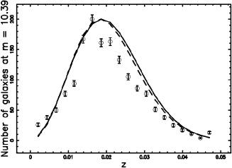
Figure 3: The galaxies of the 2MRS with $10.28\leq m\leq 10.44$ or $1202409\frac{L_{\sun}}{Mpc^{2}}\leq f\leq 1384350\frac{L_{\sun}}{Mpc^{2}}$ are organized in frequencies versus heliocentric redshift, (empty circles); the error bar is given by the square root of the frequency. The maximum frequency of observed galaxies is at $z=0.018$. The full line is the theoretical curve generated by $\frac{dN}{d\Omega dzdf}(z)$ as given by the application of the Schecter LF which is eqn.(18) and the dashed line represents the application of the Schechter LF which is eqn.(24). The parameters are the same of Table 1, $\chi^{2}=154$ for the Schechter LF and $\chi^{2}=124$ for the modified Schechter LF.

The number of all the galaxies as function of $z$ can be computed through an integral, see eqn. 23, and is visible in Figure 4.

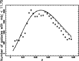
Figure 4: The same as Figure 3 but now all the galaxies are considered, $\chi^{2}=1618$ for the Schechter LF and $\chi^{2}=1352$ for the modified Schechter LF.

The maximum in the number of galaxies is at

$$z_{pos-max}(z_{crit})=\frac{\sqrt{2+\alpha}{\it z_{crit}}}{\sqrt{2\,\eta-1+\alpha\,\eta-\alpha}}\quad,$$ (25)

or

$$z_{pos-max}(f)=\frac{\sqrt{2+\alpha}\sqrt{{10}^{0.4\,{\it M_{\sun}}-0.4\,{\it M^{*}}}}H_{{0}}}{2\,\sqrt{2\,\eta-1+\alpha\,\eta-\alpha}\sqrt{\pi}\sqrt{f}{\it c_{l}}}\quad,$$ (26)

or

$$z_{pos-max}(m)=\frac{1.772\,10^{-5}\,\sqrt{2+\alpha}\sqrt{{10}^{0.4\,{\it M_{\sun}}-0.4\,{\it M^{*}}}}{\it H_{0}}}{\sqrt{2\,\eta-1+\alpha\,\eta-\alpha}\sqrt{\pi}\sqrt{{{\rm e}^{0.921\,{\it M_{\sun}}-0.921\,{\it m}}}}{\it c_{l}}}\quad.$$ (27)

0.3.3 Formulas for the generalized gamma LF

The joint distribution in z and f for galaxies when the generalized gamma LF is adopted is

$$\frac{dN}{d\Omega dzdf}=\frac{4\,{z}^{4}{{\it c_{l}}}^{5}{\it k}\,\left({\frac{{z}^{2}}{{{\it z_{crit}}}^{2}}}\right)^{{\it c}\,{\it k}-1}{{\rm e}^{-\left({\frac{{z}^{2}}{{{\it z_{crit}}}^{2}}}\right)^{{\it k}}}}{\it\Psi^{*}}\,\pi}{{H_{{0}}}^{5}{\it L^{*}}\,\Gamma\left({\it c}\right)}\quad.$$ (28)

Figure 5 reports the number of observed galaxies of the 2MRS catalog for a given apparent magnitude and two theoretical curves.

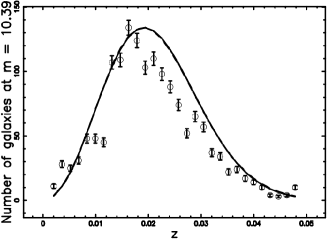
Figure 5: The same as Figure 3, the dashed line is the theoretical curve generated by $\frac{dN}{d\Omega dzdf}(z)$ as given by the application of generalized gamma LF which is eqn. (28). The parameters are the same of Table 1, $\chi^{2}=198$ for the Schechter LF and $\chi^{2}=201$ for the generalized gamma LF.

Figure 6 reports all the observed galaxies of the 2MRS.

Figure 6: The same as Figure 5 but now all the galaxies are considered, $\chi^{2}=1617$ for the Schechter LF and $\chi^{2}=1590$ for the generalized gamma LF.

The maximum in the number of galaxies is at

$$z_{pos-max}(z_{crit})={\it z_{crit}}\,\left(1+{\it c}\,{\it k}\right)^{1/2\,{{\it k}}^{-1}}{{\it k}}^{-1/2\,{{\it k}}^{-1}}\quad,$$ (29)

or

$$z_{pos-max}(f)=\frac{\sqrt{{10}^{0.4\,{\it M_{\sun}}-0.4\,{\it M^{*}}}}H_{{0}}\left(1+{\it c}\,{\it k}\right)^{1/2\,{{\it k}}^{-1}}{{\it k}}^{-1/2\,{{\it k}}^{-1}}}{\,\sqrt{\pi}\sqrt{f}{\it c_{l}}}\quad,$$ (30)

or

$$z_{pos-max}(m)=\frac{1.772\,10^{-5}\,\,\sqrt{{10}^{0.4\,{\it M_{\sun}}-0.4\,{\it M^{*}}}}H_{{0}}\left(1+{\it c}\,{\it k}\right)^{1/2\,{{\it k}}^{-1}}{{\it k}}^{-1/2\,{{\it k}}^{-1}}}{\sqrt{\pi}\sqrt{{{\rm e}^{0.921\,{\it M_{\sun}}-0.921\,{\it m}}}}{\it c_{l}}}\quad.$$ (31)

0.4 The simulation

We now simulate the 2MRS catalog adopting the framework of the Voronoi Tessellation adopting two requirements. The first requirement is that the average radius of the voids is $<R>=18.23h^{-1}$ Mpc, which is the effective radius in SDSS DR7, see Table 6 in in Zaninetti (2012). The second requirement is connected to a previous analysis which shows that the effective radius of the cosmic voids as deduced from the catalog SDSS R7 is represented by a Kiang function with $c\approx 2$. This mean that we are considering non Poissonian Voronoi Tessellation (NPVT). We briefly recall that the Poissonian Voronoi Tessellation (PVT) is characterized by a distribution of normalized volumes modeled by a Kiang function with $c\approx 5$, see Zaninetti (2012). The cross sectional area of a NPVT can also be visualized through a spherical cut characterized by a constant value of $z$ see Figure 7; this intersection is called $V_{s}(2,3)$ where the index $s$ stands for sphere.

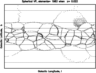
Figure 7: The Voronoi diagram $V_{s}(2,3)$ in Mercator projection when $z\approx 0.022$. Nine lines of constant latitude at latitudes -80, -60, -40,-20, 0, 20, 40, 60, 80 degrees are drawn. Each line is made up of 360 straight-line segments.

On this spherical network the galaxies are chosen according to formula (23) which represents the number of galaxies, $N_{S}(z,f_{min},f_{max})$, comprised between a minimum value of flux and maximum value of flux when the Schechter LF is considered. We have now a series of simulated spherical cuts which can be compared with the spherical cuts of 2MRS. Figure 8 reports the simulated spherical slice of galaxies at the photometric maximum.

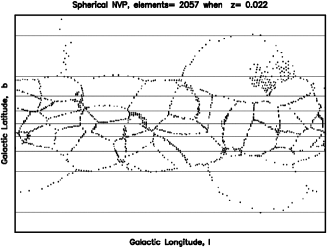
Figure 8: The Voronoi diagram $V_{s}(2,3)$ in Mercator projection when 2057 galaxies are extracted from the network of Figure 7.

A comparison can be done with the observed spherical cut of the 2MRS catalog having redshift ,$z$, corresponding to the observed photometric maximum, see Figure 9.

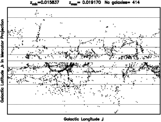
Figure 9: Mercator projection in galactic coordinates of a spherical cut of the 2MRS data at $z\approx 0.017$.

0.5 Conclusions

The most used LF in the infrared band is the Schechter LF, see eqn. (4). We have here analyzed two other LFs : the generalized gamma, see eqn. (0.2.3) and the modified Schechter LF, eqn. (8). They perform as well as the Schechter LF and the test in the $K_{s}$ band assigns to the modified Schechter LF the lowest value of the $\chi^{2}_{red}$, see Table 1. The radial distribution in the number of galaxies of 2MRS can be another test and Figure 3 and Figure 5 report the standard theoretical curve as well the two new theoretical predictions. In this case the smaller $\chi^{2}$ is given by the theoretical curve which involves the modified Schechter LF. A particular attention has been given to the position of the maximum in the number of galaxies that is here expressed as function of the theoretical parameter $z_{crit}$ or the two observable parameters $f$ and $m$. A simulation in Mercator projection of the spatial distribution of galaxies having redshift corresponding to the photometric maximum is presented, see Figure 8 .

References

• Alcaniz & Lima (2004) Alcaniz, J. S. & Lima, J. A. S. 2004, Brazilian Journal of Physics, 34, 455
• Cole et al. (2001) Cole, S., Norberg, P., Baugh, C. M., Frenk, C. S., Bland-Hawthorn, J., & Bridges, T. 2001, MNRAS  , 326, 255
• Freedman et al. (2012) Freedman, W. L., Madore, B. F., Scowcroft, V., Burns, C., Monson, A., Persson, S. E., Seibert, M., & Rigby, J. 2012, ApJ  , 758, 24
• Goto et al. (2011) Goto, T., Arnouts, S., Malkan, M., Takagi, T., & Inami, H. 2011, MNRAS  , 414, 1903
• Hubble (1929) Hubble, E. 1929, Proceedings of the National Academy of Science, 15, 168
• Huchra et al. (2012) Huchra, J. P., Macri, L. M., Masters, K. L., & et al. 2012, ApJS , 199, 26
• Keenan et al. (2012) Keenan, R. C., Barger, A. J., Cowie, L. L., Wang, W.-H., Wold, I., & Trouille, L. 2012, ApJ  , 754, 131
• Padmanabhan (2002) Padmanabhan, P. 2002, Theoretical astrophysics. Vol. III: Galaxies and Cosmology (Cambridge, MA: Cambridge University Press)
• Padmanabhan (1996) Padmanabhan, T. 1996, Cosmology and Astrophysics through Problems (Cambridge: Cambridge University Press)
• Schechter (1976) Schechter, P. 1976, ApJ  , 203, 297
• Wu et al. (2011) Wu, Y., Shi, Y., Helou, G., Armus, L., Dale, D. A., Papovich, C., Rahman, N., Dasyra, K., & Stierwalt, S. 2011, ApJ  , 734, 40
• Zaninetti (2010) Zaninetti, L. 2010, Acta Physica Polonica B, 41, 729
• Zaninetti (2012) —. 2012, Revista Mexicana de Astronomia y Astrofisica, 48, 209