Spin-orbit effects in armchair carbon nanotubes:
analytical results

Abstract

Energy spectra and transport properties of armchair nanotubes with curvature induced spin-orbit interaction are investigated thoroughly. The spin-orbit interaction consists of two terms: the first one preserves the spin symmetry in rotating frame, while the second one breaks it. It is found that the both terms are equally important: i)at scattering on the potential step which mimics a long-range potential in the nanotubes; ii)at transport via nanotube quantum dots. It is shown that an armchair nanotube with the first spin-orbit term works as an ideal spin-filter, while the second term produces a parasitic inductance.

I Introduction

Electronic and transport properties of carbon nanotubes are highly topical subjects in mesoscopic physics (see for a review b ; r1 ; r2 ; r3 ) due to potential technological applications in nano-electronics and optical devices sm ; el . Among various studies of physical properties of carbon nanotubes (CNTs), a detailed understanding of spin-orbit interaction is crucial for the interpretation of ongoing experiments as well as for future applications of the nanotubes in spintronics.

In general, the intrinsic (intraatomic) spin-orbit interaction in graphene is weak min , since carbon atoms have zero nuclear spins, and the hyperfine interaction of electron spins with nuclear spins is suppressed. It makes a spin decoherence in such material to be weak as well, i.e., scattering due to disorder is supposed to be not important. A full analysis of a spin-orbit interaction in CNTs requires, however, to consider the isospin degree of freedom present in the honeycomb carbon lattice.

According to a general wisdom, graphene being a zero-gap semiconductor has a band structure described by a linear dispersion relation at low energy, similar to massless Dirac-Weyl fermions b ; r4 . For a CNT the quantization condition leads, however, to metallic or semiconducting behavior, depending on chirality r1 ; r2 . The curved geometry may give rise to a band gap even for metallic CNTs me . Such a gap would allow to confine electrons, otherwise not possible due to the Klein paradox all . However, a precise form of a spin-orbit interaction in a single-layer graphene nanotube is still not well known.

A consistent approach to introduce the curvature-induced spin-orbit coupling (SOC) in the low-energy physics of graphene have been developed by Ando Ando and by others Ent ; Mart ; Brat . Recent measurements in ultra clean CNTs Ku , at various values of the magnetic field, revealed the energy splitting which can be associated with a spin-orbit coupling. Indeed, the measured shifts are compatible with theoretical predictions Ando ; Brat . However, some features are left debatable. Evidently, removing the degeneracy between quantum levels, the magnetic field generates new mechanisms as well, which obscure effects related to a plain spin-orbit coupling (see, for example, discussion in Loss ; Chico ; Jeo ; izum ; val ).

It is noteworthy on the pivotal fact that within the approach developed by Ando Ando one obtains two SOC terms: one preserves the spin symmetry in the rotating frame (see below), while the second one breaks this symmetry. In previous studies Ando ; Brat the role played by the second term was underestimated. The purpose of the present paper is twofold. First, to consider consistently a full curvature-induced spin-orbit coupling in an armchair nanotube within the approach suggested by Ando Ando . Second, to show that the second term could play an important role in transport phenomena. In order to illuminate the role of interplay between both terms on electron transport, we analyze the situation at zero magnetic field, removing all additional mechanisms related to the magnetic field. In contrast to previous studies, we also provide analytical estimations for the energy spectrum and transport coefficients for different cases (with and without the second term). Evidently, the analytical approach gives a fundamental insight into the nature of electronic and transport properties of CNTs.

The structure of the paper is as follows. In Sec. II we derive an explicit formula for eigen spectrum of the Ando Hamiltonian with a full curvature-induced spin-orbit coupling in an armchair nanotube. In Sec. III we discuss different symmetries associated with the Hamiltonian and analyze the current operators. Sec. IV is devoted to the analysis of scattering phenomena at the interface introduced by a potential step and to transport properties of carbon quantum dots at the preserved spin symmetry. In Sec. V, with the aid of results of Sec. IV, we discuss transport effects produced by a full curvature-induced spin-orbit coupling in armchair nanotubes. Main conclusions are summarized in Sec. VI. Appendix provides technical details used for analytical solutions.

II The Model

Figure 1 sketches a carbon nanotube and a coordinate system with respect to the orientation axis of a carbon nanotube in our analysis. The orbitals corresponding to the $\sigma$ bands of graphene are made by linear combinations of the $2s$, $2p_{x}$ $2p_{y}$ atomic orbitals, whereas the orbitals of the $\pi$ band are $p_{z}$ orbitals.

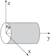
Figure 1: The coordinate system for the carbon nanotube.

Starting from the tight-binding model, with the aid of ${\bf k\cdot p}$ scheme in the vicinity of the Fermi energy ($E=0$) at $K$ and $K^{\prime}$ points of the first Brillouin Zone, Ando has derived the effective mass Hamiltonian for electrons on curved surface with spin-orbit interaction (see details in Ando ). We follow this approach and use the effective mass Hamiltonian as a starting point of our analysis. This Hamiltonian can be expressed in the form of matrix-Hamiltonian equation

$$\hat{H}\Psi=\left(\begin{array}[]{cc}0&\hat{f}\\ \hat{f}^{{\dagger}}&0\end{array}\right)\left(\begin{array}[]{c}F^{K}_{A}\\ F^{K}_{B}\end{array}\right)=E\left(\begin{array}[]{c}F^{K}_{A}\\ F^{K}_{B}\end{array}\right)\,,$$ (1)

with the following definitions

$$\hat{f}=\gamma(\hat{k}_{x}-\mathrm{i}\hat{k}_{y})+\mathrm{i}\frac{\delta\gamma^{\prime}}{4R}\hat{\sigma}_{x}(\vec{r})-\frac{2\delta\gamma p}{R}\hat{\sigma}_{y}\,,$$ (2)

$$\hat{k}_{x}=-\mathrm{i}\frac{\partial}{R\partial\theta}\,,\hat{k}_{y}=-\mathrm{i}\frac{\partial}{\partial y}\,,$$

$$\hat{\sigma}_{x}(\vec{r})=\hat{\sigma}_{x}\cos\theta-\hat{\sigma}_{z}\sin\theta\,.$$

Here, $\hat{\sigma}_{x,y,z}$ are standard Pauli matrices, and the spinors of two sub-lattices are

$$F^{K}_{A}=\left(\begin{array}[]{c}F^{K}_{A,\uparrow}\\ F^{K}_{A,\downarrow}\end{array}\right)\,,\quad F^{K}_{B}=\left(\begin{array}[]{c}F^{K}_{B,\uparrow}\\ F^{K}_{B,\downarrow}\end{array}\right)\,.$$ (3)

We preserve the definitions introduced by Ando Ando for the following parameters:

$$\gamma=-\sqrt{3}V_{pp}^{\pi}a/2\,,$$

$$\gamma^{\prime}=\sqrt{3}(V_{pp}^{\sigma}-V_{pp}^{\pi})a/2\,,$$ (4)

$$p=1-3\gamma^{\prime}/8\gamma\,.$$

Here, the quantities $V_{pp}^{\sigma}$ and $V_{pp}^{\pi}$ are the transfer integrals for $\sigma$ and $\pi$ orbitals, respectively in a flat 2D graphene, and $a$ is a lattice constant ($a=2.46$Å). The intrinsic source of the SOC $\delta={\Delta}/(3\epsilon_{\pi\sigma})$ is defined by

$$\Delta=\mathrm{i}\frac{3\hbar}{4m_{e}^{2}c^{2}}\langle x_{l}|\frac{\partial V}{\partial x}\hat{p}_{y}-\frac{\partial V}{\partial y}\hat{p}_{x}|y_{l}\rangle$$ (5)

and $\epsilon_{\pi\sigma}=\epsilon_{2p}^{\pi}-\epsilon_{2p}^{\sigma}$, where $V$ is the atomic potential. The energy $\epsilon_{2p}^{\sigma}$ is the energy of $\sigma$-orbitals which are localized between carbon atoms. The energy $\epsilon_{2p}^{\pi}$ is the energy of $\pi$-orbitals which are directed perpendicular to the nanotube surface. In our consideration $x_{l}$, $y_{l}$, and $z_{l}$ are local coordinates; $z_{l}$-axis is perpendicular to a graphene plane, and $y_{l}$-axis is lying along the tube symmetry axis.

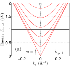
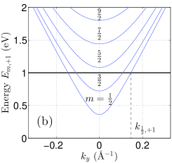
Figure 2: (Color online) Positive spectrum (see Eqs.(A.22)) $E_{m,-1}$ (a) and $E_{m,+1}$ (b) as a function of the wave number $k_{y}$. The values of $k_{m,+1}$ and $k_{m,-1}$ for $m=1/2$ at the energy $E_{F}=1$eV (solid horizontal line) are indicated by vertical dashed lines. The parameters are $R=17.75$Å, $\delta=0.01$, $p=0.1$, $\gamma=\frac{9}{2}1.42$ÅeV, $\gamma^{\prime}=\gamma\frac{8}{3}$, $\lambda_{x}=\frac{\gamma}{R}(1/2+2\delta p)=0.18$eV, $\lambda_{y}=\frac{\delta\gamma^{\prime}}{4R}=0.0024$eV.

Ando suggested to neglect a spin-orbit term proportional to $\sigma_{x}$, i.e., the term $\delta\gamma^{\prime}/(4R)\hat{\sigma}_{x}(\vec{r})$ in the Hamiltonian (1). He assumed that a spin projection on the CNT symmetry axis (y-axis) is a conserved integral of motion. Based on the perturbative approach result, he concluded that a spin mixing in the wave function due to this term is very small. Ando admitted, however, that it may couple states from bands with different spin quantum numbers and lead to a small spin relaxation. Although in Ref.izum a different basis was used to derive the effective Hamiltonian for a single wall CNT, the term breaking its spin symmetry (a conservation of ${\hat{s}_{z}}$-component) was obtained as well. Similar to Ref.Ando , it was also suggested in Ref.izum to neglect such a term. In contrast, we consider all spin-orbit terms on equal footing, since even a small perturbation brought about by the second term breaks the fundamental spin symmetry of the total Hamiltonian. In this case all three spin projections are not conserved in any system. Different bands must be distinguished by the magnetic quantum number $m$ which is a projection of the total angular momentum on the symmetry axis of the CNT (see below). As a result, this preserved fundamental symmetry allows to couple states with different spins even inside one band. We restrict our consideration by an armchair nanotube. In this case the SOC does not lead to the additional effect such as an electron-hole asymmetry izum ; val .

To get rid of the $\theta$ dependence in the Hamiltonian (1), we apply the transformation

$$\hat{H}^{\prime}=\hat{U}\hat{H}\hat{U}^{-1}$$ (6)

with the aid of the unitary operator $\hat{U}$

$$\hat{U}=\left(\begin{array}[]{cc}\exp({\mathrm{i}\frac{\theta}{2}}\hat{\sigma}_{y})&0\\ 0&\exp({\mathrm{i}\frac{\theta}{2}}\hat{\sigma}_{y})\end{array}\right)\,.$$ (7)

As a result, we obtain the Hamiltonian in the transformed frame

$$\hat{H}^{\prime}=\hat{H}_{\it kin}+\hat{H}_{SOC}\,,$$ (8)

$$\hat{H}_{\it kin}=-\mathrm{i}\gamma\left(\hat{\tau}_{y}\otimes I\partial_{y}+\hat{\tau}_{x}\otimes I\frac{1}{R}\partial_{\theta}\right)\,,$$ (9)

$$\hat{H}_{SOC}=-\lambda_{y}\hat{\tau}_{y}\otimes\hat{\sigma}_{x}-\lambda_{x}\hat{\tau}_{x}\otimes\hat{\sigma}_{y}\,,$$ (10)

where $I$ is $2\times 2$ unity matrix, and

$$\lambda_{x}=\gamma\left(1+4\delta p\right)/(2R)\,,\quad\lambda_{y}=\delta\gamma^{\prime}/(4R)\,.$$ (11)

We distinguish in the Hamiltonian (8) the kinetic $\hat{H}_{\it kin}$ and the potential $\hat{H}_{SOC}$ terms. Here, the operators $\hat{\tau}_{x,y,z}$ are the Pauli matrices which act on the wave functions of A- and B-sub-lattices (a pseudo-spin space). Note that the kinetic term couples the wave functions of A- and B-sub-lattices as well as the potential term.

In our consideration, the curvature-induced spin-orbit coupling is described by two terms: $\lambda_{x}$ and $\lambda_{y}$. The term $\lambda_{x}$ depends on: i)values of the transfer integral $V_{pp}^{\pi}$ for $\pi$ orbitals; and ii)combined action produced by a product of the intrinsic spin-orbit interaction and the difference between the transfer integrals $V_{pp}^{\pi}$, $V_{pp}^{\sigma}$ for $\pi$ and $\sigma$ orbitals, respectively, in a flat 2D graphene. The term $\lambda_{y}$ depends on the difference between the transfer integrals $V_{pp}^{\pi}$, $V_{pp}^{\sigma}$ for $\pi$ and $\sigma$ orbitals, respectively, in a flat 2D graphene. The both terms are inversely proportional to the tube radius, and tend to zero at $R\to\infty$, i.e., in the limit of a flat graphene. For small nanotubes (small radius) we might expect, however, that effects produced by these terms come into particular prominence in transport phenomena.

Herewith, for the sake of convenience, we use $\hbar=1$, if otherwise it will be not mentioned. At $\lambda_{y}=0$, the spin projection $\hat{S}_{y}=\frac{1}{2}I\otimes\hat{\sigma}_{y}$ is a constant of motion, since it commutes with the Hamiltonian $[\hat{S}_{y},\hat{H}^{\prime}]=0$. The term $\lambda_{y}\neq 0$ breaks this symmetry and yields a spin mixing. Due to an axial symmetry of the CNT, the projection of a total angular momentum on the nanotube symmetry axis is always the integral of motion. In our consideration, in the transformed system the integral of motion $\hat{J}_{y}$

$$\hat{J}_{y}=I\otimes\left(\hat{L}_{y}+\frac{\hat{\sigma}_{y}}{2}\right)=I\otimes\left(-\mathrm{i}\partial_{\theta}+\frac{\hat{\sigma}_{y}}{2}\right),\;\left[\hat{H},\hat{J}_{y}\right]=0$$ (12)

takes a simple form

$$\hat{J}_{y}\rightarrow\hat{J}_{y}^{\prime}=\hat{U}\hat{J}_{y}\hat{U}^{-1}=I\otimes\left(-\mathrm{i}\partial_{\theta}\right).$$ (13)

In virtue of this fact, we consider the wave function in the form of plane waves

$$F^{\prime}(\theta,y)=e^{\mathrm{i}m\theta}e^{\mathrm{i}k_{y}y}\Psi\,,$$ (14)

where the wave function $\Psi$ is a four-component spinor. The wave function (14) defines the eigenvalues $m$ of the operator $\hat{J}_{y}$

$$\hat{J}_{y}^{\prime}F^{\prime}(\theta,y)=mF^{\prime}(\theta,y)\,,m=\pm 1/2,\pm 3/2,....,$$ (15)

while a quantum number $k_{y}$ is an eigenvalue of the operator $\hat{k}^{\prime}_{y}\equiv\hat{k}_{y}$

$$\hat{k}_{y}^{\prime}F^{\prime}(\theta,y)=k_{y}F^{\prime}(\theta,y)\,.$$ (16)

Taking into account Eqs.(8,14), we obtain our Hamiltonian

$$\hat{H}^{\prime}(m,k_{y})=$$ (17)

$$\left(\begin{array}[]{cccc}0&0&t_{m}-\mathrm{i}t_{y}&\mathrm{i}(\lambda_{y}+\lambda_{x})\\ 0&0&\mathrm{i}(\lambda_{y}-\lambda_{x})&t_{m}-\mathrm{i}t_{y}\\ t_{m}+\mathrm{i}t_{y}&-\mathrm{i}(\lambda_{y}-\lambda_{x})&0&0\\ -\mathrm{i}(\lambda_{y}+\lambda_{x})&t_{m}+\mathrm{i}t_{y}&0&0\\ \end{array}\right),$$ (22)

which acts on the spinor $\Psi$. Here we introduce the following definitions

$$t_{m}=\frac{\gamma}{R}m,\;t_{y}=\gamma k_{y}.$$ (23)

The solution of the eigenvalue problem of Hamiltonian (17) yields the following four energies (see Appendix A, Eqs.(A.22))

$$E^{(+)}=+E_{m,s}\,,E^{(-)}=-E_{m,s}\,,\quad s=\pm 1.$$ (24)

We define all states with $E^{(+)}>0$ ($E^{(-)}<0$) as a particle (hole) states. As was mentioned above, there is the electron-hole symmetry $|E^{(+)}|=|E^{(-)}|$.

The energy spectrum for a typical CNT as a function of the continuous variable $k_{y}$ and the quantized projection of the angular momentum $m$ is shown on Fig.2. For the sake of illustrations, in numerical calculations we use the following parameters Ando : $V_{pp}^{\pi}\sim-3$eV, $V_{pp}^{\sigma}\sim 5$eV, $|p|\sim 0.1$, the bond length $d=a/\sqrt{3}\approx$ 1.42Å. For a given $m$-value the Fermi energy $E_{F}$ provides four possible values for $k_{y}$: $\pm k_{m,s}$.

The energy gap $\Delta E_{m,s}$ in the CNT is defined by a minimal distance between negative and positive parts of the spectrum (see Eqs.(A.22))

$$\Delta E_{m,s}=2|E_{m,s}(k_{y}=0)|=2\left|\sqrt{t_{m}^{2}+\lambda_{y}^{2}}+s\lambda_{x}\right|\equiv 2E^{0}_{m,s}\,.$$ (25)

At $\lambda_{y}=0$ there is a minimal gap $\Delta E_{1/2,-1}=4\gamma\delta|p|/R$, which coincides with the value obtained by Ando Ando . At $\lambda_{x}\neq 0$ and $\lambda_{y}\neq 0$ for $p>0$ the minimal gap becomes even lesser, while for $p<0$ it increases. Thus, the comparison of the gap (25) with experimental data would allow to fix the model parameters (II). The transport does not persist in the gap, since all eigen modes are evanescent ones. Evidently, when the spin-orbit interaction ($\delta=0$) is zero, one is faced with a plain metallic CNT.

III Symmetries and current operators

The Hamiltonian (8) has several symmetries. There is a particle-hole symmetry

$$\hat{M}_{a}\hat{H}^{\prime}\hat{M}_{a}^{-1}=-\hat{H}^{\prime}\,,$$ (26)

defined by the operator

$$\hat{M}_{a}=\hat{\tau}_{z}\otimes I\,.$$ (27)

Therefore, energies for the eigenfunctions $\Psi$ and $\hat{M}_{a}\Psi$ are equal in value but opposite in sign. There are two inversion operators $M_{\theta}$, $M_{y}$, for $\theta$, $y$ coordinates, respectively,

$$\hat{M}_{y}=\hat{\tau}_{y}\otimes\hat{\sigma}_{y}\,,\quad\hat{M}_{\theta}=\hat{\tau}_{y}\otimes\hat{\sigma}_{x},$$ (28)

with properties

$$\hat{M}_{y}\hat{H}^{\prime}(\hat{k}_{y},\hat{J}_{y})\hat{M}_{y}^{-1}=\hat{H}^{\prime}(-\hat{k}_{y},\hat{J}_{y})\,,$$ (29)

$$\hat{M}_{\theta}\hat{H}^{\prime}(\hat{k}_{y},\hat{J}_{y})\hat{M}_{\theta}^{-1}=\hat{H}^{\prime}(\hat{k}_{y},-\hat{J}_{y})\,.$$ (30)

These transformations connect the eigenfunctions with opposite quantum numbers $k_{y}$ and $m$.

In virtue of the conservation law for the current ${\bf j=j_{y}+j_{\theta}}$

$$\frac{\partial}{\partial t}|\Psi|^{2}+\nabla{\bf j}=0\,,$$ (31)

we obtain a longitudinal and an orbital current operators

$$\hat{j}_{y}=\gamma\hat{\tau}_{y}\otimes I\,,\quad\hat{j}_{\theta}=\gamma\hat{\tau}_{x}\otimes I.$$ (32)

The same expressions can be obtained from the equation of motion

$$\hat{v}=\hat{\dot{r}}=\mathrm{i}[\hat{H}^{\prime},\hat{r}]\,.$$ (33)

For fixed quantum numbers $(k_{y},m)$, at $E>0$ the current moves in a direction opposite to one of the current at $E<0$. This fact follows from the symmetry relation

$$\hat{M}^{-1}_{a}\hat{j}_{y,\theta}\hat{M}_{a}=-\hat{j}_{y,\theta}\,.$$ (34)

The expectation values of the $\theta$ ($y$)-component of the current calculated by means of the eigenfunctions $\Psi$ and $M_{\theta}\Psi$ ($M_{y}\Psi$) are of opposite sign. This result follows from the identities

$$\hat{M}^{-1}_{\theta}\hat{j}_{\theta}\hat{M}_{\theta}=-\hat{j}_{\theta}\,,\quad\hat{M}^{-1}_{y}\hat{j}_{\theta}\hat{M}_{y}=\hat{j}_{\theta}\,,$$ (35)

$$\hat{M}^{-1}_{\theta}\hat{j}_{y}\hat{M}_{\theta}=\hat{j}_{y}\,,\quad\hat{M}^{-1}_{y}\hat{j}_{y}\hat{M}_{y}=-\hat{j}_{y}\,.$$ (36)

With the aid of the relations

$$\hat{M}^{-1}_{\theta}\hat{S}_{y,z}\hat{M}_{\theta}=-\hat{S}_{y,z}\,,$$ (37)

$$\hat{M}^{-1}_{\theta}\hat{S}_{x}\hat{M}_{\theta}=\hat{S}_{x}\,,$$ (38)

$$\hat{M}^{-1}_{y}\hat{S}_{x,z}\hat{M}_{y}=-\hat{S}_{x,z}\,,$$ (39)

$$\hat{M}^{-1}_{y}\hat{S}_{y}\hat{M}_{y}=\hat{S}_{y}\,,$$ (40)

it could be shown that the expectation values of spin projections onto the local $y,z$ ($x,z$)-axes for the eigenfunctions $\Psi$ and $M_{\theta}\Psi$ ($M_{y}\Psi$) have also opposite signs.

IV Analytical results at $\lambda_{y}=0$

To understand how the full SOC affects the system properties, we consider first only $\lambda_{x}\neq 0$, $\lambda_{y}=0$. As discussed above, in this case the operator $\hat{S}_{y}=\frac{1}{2}I\otimes\hat{\sigma}_{y}$ is an integral of motion. Therefore, we transform our Hamiltonian to the frame where the operator $\hat{S}_{y}$ has a diagonal form

$$\hat{\cal V}^{-1}\hat{S}_{y}\hat{\cal V}=\frac{1}{2}\hat{\sigma}_{z}\otimes I\,.$$ (41)

Here, the transformation $\hat{\cal V}$, defined as

$$\hat{\cal V}=\left(\exp\left(\mathrm{i}\frac{\pi}{4}\hat{\sigma}_{x}\right)\otimes I\right)\hat{P}_{23}\,,\hat{P}_{23}=\left(\begin{array}[]{cccc}1&0&0&0\\ 0&0&1&0\\ 0&1&0&0\\ 0&0&0&1\end{array}\right)\,,$$ (42)

consists of a rotation on angle $\pi/2$ around $x$-axis and the permutation $P_{23}$. This permutation collects spin up components of the A- and B-sub-lattices in the upper part of the spinor $\Psi$. In virtue of this transformation, the Hamiltonian (17) gains a block-diagonal structure

$$\hat{\cal H}=\hat{\cal V}^{-1}\hat{H}^{\prime}\hat{\cal V}=\left(\begin{array}[]{cccc}0&a_{-}&0&0\\ a_{+}&0&0&0\\ 0&0&0&b_{-}\\ 0&0&b_{+}&0\end{array}\right)\,,$$ (47)

$$a_{\pm}=(t_{m}-\lambda_{x})\pm\mathrm{i}t_{y}\,,\quad b_{\pm}=(t_{m}+\lambda_{x})\pm\mathrm{i}t_{y}\,.$$

One obtains obvious four eigenvalues and eigenvectors

$$E^{(\pm)}=\pm E_{m,s},\quad E_{m,s}=\sqrt{(t_{m}+s\lambda_{x})^{2}+t_{y}^{2}}\,,$$ (48)

$$V_{m,+1}=\frac{1}{\sqrt{2}}(0,0,1,z_{m,+1})^{T}\,,$$ (49)

$$V_{m,-1}=\frac{1}{\sqrt{2}}(1,z_{m,-1},0,0)^{T}\,,$$ (50)

$$\quad z_{m,s}=((t_{m}+s\lambda_{x})+\mathrm{i}t_{y})/E\,.$$ (51)

IV.1 Scattering on a potential step

We consider first the scattering at the interface introduced by a potential step of the height $V_{0}$ as sketched in Fig.3. On the one hand, the step is assumed to be smooth on the length scale of a graphene unit cell (an inverse Brillouin momentum $2\pi/K$). Therefore, it does not induce the intervalley ($K\to K^{\prime}$) scattering. On the other hand, it is assumed to be sharp on the Fermi length scale ($\lambda\sim 1/k_{F}$). Since $\theta$ and $y$ are independent variables, such a potential conserves the angular momentum projection $m$.

Depending on the sign of $E_{F}$ (incoming particle) and the sign of $E_{F}-V_{0}$ (outgoing particle) there are four types of transmission through the step: p-p, p-h, h-p, h-h. We denote particle by symbol ”p”, while a hole by a symbol ”h”. For the sake of illustration, p-p and p-h transmissions are schematically shown on Fig.3.

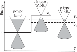
Figure 3: A schematic illustration of the scattering process on a potential step.

Transmission (reflection) of electrons incoming from the left is controlled by partial coefficients. Namely, we have $|t^{q}_{q^{\prime}}|^{2}(|r^{q}_{q^{\prime}}|^{2})$ describing transmission (reflection) probability from the left states with a set of quantum numbers $q=\{m,s\}$ to the right states with $q^{\prime}=\{m^{\prime},s^{\prime}\}$. Transmission (reflection) probabilities are defined as squares of the scattering-wave-function amplitudes which satisfy the continuity of wave functions. Evidently, since spin is a good quantum number as well as a quantum number $m$, the transmission (reflection) probabilities, responsible for the spin-flip process, are absent at $\lambda_{y}=0$: $|t^{m,s}_{m,s^{\prime}}|^{2}=|r^{m,s}_{m,s^{\prime}}|^{2}=0$ for $s\neq s^{\prime}$.

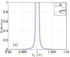
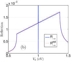
Figure 4: (Color online) Reflection probabilities on the potential step for the state $m=1/2$, $s=-1$: analytical estimation (dotted line, red) and numerical results (solid line, blue) as a function of the potential height $V_{0}$. (a) $\lambda_{y}=0$ : a direct reflection $R_{--}^{\rm est}(V_{0})=|r_{m,s}^{m,s}(V_{0})|^{2}$ is described by Eq.(56); (b) $\lambda_{y}\neq 0$: a spin-flip reflection $R_{-+}^{\rm est}(V_{0})=|r_{m,-s}^{m,s}(V_{0})|^{2}$ is described by Eq.(87). $E_{F}=1$eV and the other parameters are the same as in Fig.2.

Matching the eigenfunctions with the same values of the angular momentum and spin projections on the left and right sides of the potential step, we obtain the following equation

$$\frac{\left[\left(\begin{array}[]{c}1\\ Z_{q}\end{array}\right)+r_{q}^{q}\left(\begin{array}[]{c}1\\ Z_{q}^{-1}\end{array}\right)\right]}{\sqrt{|\gamma\mathrm{i}(z_{q}^{*}-z_{q})|}}=\frac{t_{q}^{q}}{\sqrt{|\gamma\mathrm{i}({\tilde{z}}_{q}^{*}-{\tilde{z}}_{q})|}}\left(\begin{array}[]{c}1\\ {\tilde{Z}}_{q}\end{array}\right).$$ (52)

Here $Z_{q}=(z_{q})^{{\rm sign}(E_{F})}$ (${\tilde{Z}}_{q}=({\tilde{z}_{q}})^{{\rm sign}(E_{F}-V_{0})}$) are defined by Eq.(51), $z_{q}^{*}$ (${\tilde{z}}_{q}^{*}$) are complex conjugate, and the energy $E=E_{F}$ ($E=E_{F}-V_{0}$) before (after) the step. The wave functions are normalized to have a unit current flow along the $y$-axis. The solution of Eq.(52) defines the reflection and transmission coefficients

$$r_{q}^{q}=(Z_{q}-{\tilde{Z}}_{q})/({\tilde{Z}}_{q}-Z_{q}^{-1})\,,$$ (53)

$$t_{q}^{q}=(Z_{q}-Z_{q}^{-1})/({\tilde{Z}}_{q}-Z_{q}^{-1})\sqrt{\left|\frac{{\tilde{z}}_{q}-{\tilde{z}}_{q}^{*}}{z_{q}-z_{q}^{*}}\right|}\,.$$ (54)

In order to reveal the effect of the SOC let us consider the case of quantum numbers $q_{n}:\{m=\mp\frac{1}{2},s=\pm 1\}$. It corresponds to a normal incident direction of electrons on the potential step for the CNT without the SOC and $\delta=0$. Note that the variable $z_{q}$ (${\tilde{z}}_{q}$) (see Eq.(51)) depends on the term $t_{m}+s\lambda_{x}$. In our case this term transforms to the form

$$t_{m}+s\lambda_{x}=\frac{\gamma}{R}\left(m+s/2+2sp\delta\right)\Rightarrow\pm\frac{\gamma}{R}2p\delta\,,$$ (55)

which depends on a small parameter $\delta$. The Taylor series expansion of the reflection $r_{q_{n}}^{q_{n}}$ (see Eq.(53)) over this parameter $\delta$ enables to us to define the first nonzero term (omitting unimportant phase factor)

$$r_{q_{n}}^{q_{n}}=\delta p\frac{\gamma}{R}\frac{V_{0}}{E_{F}(E_{F}-V_{0})}+O(\delta^{2})\,.$$ (56)

The estimation (56) describes remarkably well numerical results for the scattering until $E_{F}$ or $E_{F}-V_{0}$ is close to the gap (see Fig.4a). Thus, at $|E_{F}|\gg E_{q_{n}}^{0}$ and $|E_{F}-V_{0}|\gg E_{q_{n}}^{0}$, where $E_{q_{n}}^{0}=2|\delta p\gamma|/R$ is of order $10^{-4}$eV for the typical parameters of CNTs, there is a weak backward scattering defined by Eq. (56).

To gain a better insight into scattering phenomena we study the current. At $\lambda_{y}=0$ the expectation value of the longitudinal current $\langle\hat{j}_{y}\rangle$ is determined by the quantum number $k_{y}$. The effect of the SOC is visible in the expectation value of the orbital ($\theta$-) component of the current (see Appendix A, Eq.(A))

$$\langle\hat{j}_{\theta}\rangle_{q}=\frac{\gamma}{E}\left(t_{m}+s\lambda_{x}\right)\,,$$ (57)

which depends on the spin-orbit term $\lambda_{x}$. With the aid of Eqs.(11), (23), one obtains that the orbital current is always nonzero. Thus, we can have a persistent current without a magnetic field. In order to understand this result let us assume that there is a magnetic field along the symmetry axis $y$. It results in the Aharonov-Bohm magnetic flux passing through the CNT cross section, which yields the modified quantum number $m^{\prime}=m+\phi/\phi_{0}$ ($\phi$ – magnetic flux, $\phi_{0}$ – magnetic flux quanta). Evidently, with the aid of the magnetic field along the symmetry axis y one can suppress the orbital current for any value of the quantum number $m$ (without the Zeeman splitting). Taking into account Eqs.(11), (23), (57), we obtain the condition for a zero orbital current for a magnetic quantum number $m$

$$t_{m^{\prime}}=-s\lambda_{x}\Rightarrow\phi/\phi_{0}=-(\frac{s}{2}+m)-2s\delta p\,.$$ (58)

In particular, for the set of quantum numbers $q_{n}=\{m=\mp\frac{1}{2},s=\pm 1\}$ we obtain $\langle\hat{j}_{\theta}\rangle_{q}=0$ at the magnetic flux $\phi/\phi_{0}=-2s\delta p$ which compensates the SOC term $\lambda_{x}$ at $m=-1/2$. Note that at the condition (58) (and $\lambda_{y}=0$) the gap (25) vanishes as well for any $m$.

Thus, the SOC works as an ”effective magnetic field”, responsible for the orbital motion and, therefore, for the weak backward scattering (56). In the absence of Zeeman splitting the applied magnetic field $\phi/\phi_{0}=-2s\delta p$ leads to zero backward scattering in all orders.

IV.2 Quantum dot

The gap in CNTs (due to the SOC) opens a possibility to create a nanotube quantum dot (QD), by confining particles in a quantum well with a potential $V_{0}(\theta(y)-\theta(L-y))$ (where $\theta(x)$ is a Heaviside step functions), as illustrated in Fig.5. We recall that in the gap there are evanescent modes only.

The QD energies are located within the gap $-E_{q}^{0}<E<E_{q}^{0}$ (see Eq. (25)). Different sets of quantum numbers $q=\{m,s\}$ determine the full spectrum of the QD. Matching the eigenfunctions (49) at the $y=0$ and $y=L$ we obtain the following equations

$$r_{l}\left(\begin{array}[]{c}1\\ z_{q}^{-1}\end{array}\right)=a\left(\begin{array}[]{c}1\\ {\tilde{z}}_{q}\end{array}\right)+b\left(\begin{array}[]{c}1\\ {\tilde{z}}_{q}^{-1}\end{array}\right)\,,$$ (65)

$$r_{r}\left(\begin{array}[]{c}1\\ z_{q}\end{array}\right)=ae^{\mathrm{i}k_{q}(E)L}\left(\begin{array}[]{c}1\\ {\tilde{z}}_{q}\end{array}\right)+be^{-\mathrm{i}k_{q}(E)L}\left(\begin{array}[]{c}1\\ {\tilde{z}}_{q}^{-1}\end{array}\right)\!\!\!,$$ (72)

where

$$z_{q}(E)=\left[(t_{m}+s\lambda_{x})-\kappa_{q}(E)\gamma\right]/E\,,$$

$$\kappa_{q}(E)=\sqrt{(t_{m}+s\lambda_{x})^{2}-E^{2}}/\gamma\,,$$

$${\tilde{z}}_{q}(E)=\left[(t_{m}+s\lambda_{x})+\mathrm{i}k_{q}(E)\gamma\right]/(E-V_{0})\,,$$ (73)

$$k_{q}(E)=\sqrt{(E-V_{0})^{2}-(t_{m}+s\lambda_{x})^{2}}/\gamma\,.$$

These equations could be written in the matrix form

$$\left(\begin{array}[]{cccc}-1&1&1&0\\ -z_{q}^{-1}&{\tilde{z}}_{q}&{\tilde{z}}_{q}^{-1}&0\\ 0&e^{\mathrm{i}k_{q}(E)L}&e^{-\mathrm{i}k_{q}(E)L}&-1\\ 0&{\tilde{z}}_{q}e^{\mathrm{i}k_{q}(E)L}&{\tilde{z}}_{q}^{-1}e^{-\mathrm{i}k_{q}(E)L}&-z_{q}\end{array}\right)\,\left(\begin{array}[]{c}r_{l}\\ a\\ b\\ r_{r}\end{array}\right)=0$$ (74)

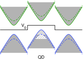
Figure 5: (Color online) A schematic picture of quantum dot in CNT. Dashed lines correspond to different sets of conserved quantum numbers.

Evidently, the solutions exist, if the determinant of Eq.(74) is zero. This requirement yields the transcendental equation which defines the eigen spectrum $E_{q}^{n}$ of the QD:

$$\exp(2\mathrm{i}k_{q}(E_{q}^{n})L)=\left(\frac{z_{q}(E_{q}^{n}){\tilde{z}}_{q}(E_{q}^{n})-1}{z_{q}(E_{q}^{n})-{\tilde{z}}_{q}(E_{q}^{n})}\right)^{2}\,,\quad n=1,2,3...$$ (75)

Eq.(75) can be transformed to the form

$$\tan(k_{q}(E_{q}^{n})L)=\left(\frac{\gamma^{2}k_{q}(E_{q}^{n})\kappa_{q}(E_{q}^{n})}{E_{q}^{n}(E_{q}^{n}-V_{0})-(t_{m}+s\lambda_{x})^{2}}\right).$$ (76)

As it was mentioned above, the QD spectrum is defined in the energy window $-E_{q}^{0}<E_{q}^{n}<E_{q}^{0}$. Its boundaries are shown on Fig. 6. Thus, Eq.(76) corresponds to the case $\lambda_{y}=0$, when there is no spin scattering. In other words, in such QDs an electron with spin up cannot scatter into a state with spin down and vise versa, without any additional mechanism.

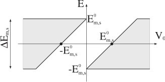
Figure 6: Grey regions correspond to the area where discrete spectrum is possible.

In order to gain a better insight into the properties of the QD spectrum, let us consider two limiting cases: a) $\gamma k_{q}(E_{q}^{n})\gg|t_{m}+s\lambda_{x}|$ ; and b) $\gamma k_{q}(E_{q}^{n})\ll|t_{m}+s\lambda_{x}|$. In case a), with the aid of Eq.(IV.2) we have

$$\gamma k_{q}(E_{q}^{n})\approx|E_{q}^{n}-V_{0}|\gg t_{m}+s\lambda_{x}\,,\quad z_{q}(E_{q}^{n})\approx\pm\mathrm{i}\,.$$ (77)

As a result, Eq. (75) transforms to the form

$$\exp\left(2\mathrm{i}\frac{|E_{q}^{n}-V_{0}|}{\gamma}L\right)\approx\left(\frac{\pm\mathrm{i}{\tilde{z}}_{q}(E_{q}^{n})-1}{\pm\mathrm{i}-{\tilde{z}}_{q}(E_{q}^{n})}\right)^{2}\approx const.\,.$$ (78)

At the condition $E_{q}^{n+1}-E_{q}^{n}\ll V_{0}$ it yields an equidistant spectrum, similar to the one of the harmonic oscillator potential:

$$E^{n+1}_{q}-E^{n}_{q}\approx\frac{\gamma\pi}{L}.$$ (79)

In case b), at small $k_{q}(E_{q}^{n})$ we obtain

$$\gamma k^{n}_{q}(E_{q}^{n})=\sqrt{(E_{q}^{n}-V_{0})^{2}-(t_{m}+s\lambda_{x})^{2}}\ll t_{m}+s\lambda_{x}\,,$$

$$\quad z_{q}(E_{q}^{n})\approx\pm 1\,.$$ (80)

As a result, Eq. (75) takes the form

$$\exp\left(2\mathrm{i}k^{n}_{q}(E_{q}^{n})L\right)\approx 1\,.$$ (81)

At the condition $E_{q}^{n+1}-E_{q}^{n}\ll t_{m}+s\lambda_{x}$ it defines the spectrum similar to the one of the quantum well potential:

$$E^{n+1}_{q}-E^{n}_{q}\approx\left(\frac{\gamma\pi}{L}\right)^{2}\frac{2n+1}{2(t_{m}+s\lambda_{x})}\,.$$ (82)

Both limits (low-and high-energies) should be fulfilled for long nanotubes.

V General case

V.1 Scattering on a potential step

Analytical solutions of the eigenvalue problem for the Hamiltonian (17) with nonzero $\lambda_{x}$ and $\lambda_{y}$ are presented in Appendix A. With the aid of these results we reconsider the scattering at the interface introduced by a potential step of the height $V_{0}$ (Fig.3). Unfortunately, analytical expressions for the general case are too cumbersome, and we present mostly numerical results. We use the same typical values for graphene nanotubes (as in the previous section) to demonstrate a general tendency.

The expectation value of the orbital ($\theta$) current component (see Appendix A, Eq.(A))

$$\langle\hat{j}_{\theta}\rangle_{m,s}=\frac{\gamma t_{m}}{E}\left(1+s\frac{\lambda_{x}^{2}}{\sqrt{\lambda_{x}^{2}(t_{m}^{2}+\lambda_{y}^{2})+t_{y}^{2}\lambda_{y}^{2}}}\right)$$ (83)

essentially depends on the spin-orbit term $\lambda_{y}\neq 0$, ignored in literature (see Fig.7).

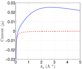
Figure 7: (Color online) Current $\langle\hat{j}_{\theta}\rangle_{q}$ (see Eq.(83)) as a function of the wave number $k_{y}$ for the eigenstate with $q=\{m=1/2,s=-1\}$ at $\lambda_{x}\neq 0$ for: $\lambda_{y}\neq 0$ (solid line) and $\lambda_{y}=0$ (dashed line). The other parameters are the same as in Fig.2. At $k_{y}\approx 0.19$Å^-1 the current is zero.

The orbital current becomes zero at

$$|m|=1/2\,,s=-1\,,|t_{y}|=\frac{\lambda_{x}}{\lambda_{y}}\sqrt{\lambda_{x}^{2}-\lambda_{y}^{2}-t_{m}^{2}}\,,$$ (84)

which corresponds to the energy $E=\pm 1.199$eV for the parameters listed in the caption of Fig.2. To avoid the additional back scattering due to non-normal incidence of electrons on the potential step, we use this energy and the quantum number $m=1/2$ for incoming electron to trace the transmission and reflection events as a function of $V_{0}$ (Fig.8). For energies $E-V_{0}\leq 0.5$eV the conductance

$$G=\frac{e^{2}}{h}(|t^{m,+1}_{m,+1}|^{2}+|t^{m,-1}_{m,-1}|^{2}+|t^{m,+1}_{m,-1}|^{2}+|t^{m,-1}_{m,+1}|^{2})$$ (85)

is dominated by the transmission without spin-flip (see Fig.8a,c), i.e., by the probabilities $T_{++}=|t^{m,+1}_{m,+1}|^{2}$ and $T_{--}=|t^{m,-1}_{m,-1}|^{2}$, while the reflection is suppressed. At $E-V_{0}>0.5$eV the SOC gives rise to the direct reflection $R_{++}=|r^{m,+1}_{m,+1}|^{2}$ (without spin-flip), which grows rather rapidly. Within the energy gap $-E_{m,+1}^{0}<E_{F}-V_{0}<-E_{m,-1}^{0}$ and $E_{m,-1}^{0}<E_{F}-V_{0}<E_{m,+1}^{0}$ ($E_{1/2,+1}^{0}\approx 0.36$eV) the transmission probability $T_{--}\approx 1$, while the transmission probability $T_{++}$ is almost suppressed, since the reflection probability $R_{++}\approx 1$. Although the probability $T_{--}$ is a dominant process, the probability $T_{+-}=|t^{m,+1}_{m,-1}|^{2}$ produces a parasitic loss of this dominance due to $\lambda_{y}$ term in the SOC. Note that the transmission probability $T_{-+}=|t^{m,-1}_{m,+1}|^{2}$ is completely suppressed in this energy window.

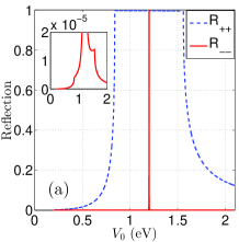
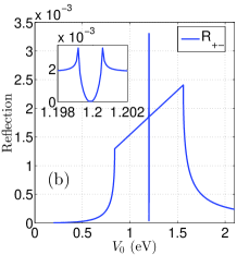
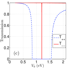
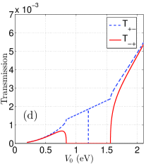
Figure 8: (Color online) Dependence of reflection (a), (b) and transmission (c), (d) probabilities for normal incidence at $m=1/2$, $E_{F}=1.199$eV on the height of the potential step $V_{0}$ (eV). The parameters are the same as in Fig.2.

This mechanism resembles in appearance to the one considered for one-dimensional electron system formed in semiconductor heterostructures showing strong Rashba spin-orbit interaction in the presence of weak magnetic field SebaPRL2003 . In our case, the spin-filter effect is brought about by a relatively weak curvature-induced SOC which creates the ”effective magnetic field”. It is noteworthy that at $\lambda_{y}=0$ the filter would be even more efficient due to the absence of the inter-channel scattering.

There is a full reflection zone which corresponds to the SOC’s induced gap of the width $\Delta E_{1/2,-1}=2*0.7meV\approx 16^{\circ}K$ for chosen parameters. In this energy interval the evanescent modes exist only. In contrast to the case considered in the previous section ($\lambda_{y}=0$), there is a mixing of spin components. In general, the back scattering

$$G_{bs}=\frac{e^{2}}{h}(|r^{m,+1}_{m,+1}|^{2}+|r^{m,-1}_{m,-1}|^{2}+|r^{m,+1}_{m,-1}|^{2}+|r^{m,-1}_{m,+1}|^{2})$$ (86)

being small increases on two order in magnitude in the presence of the SOC induced by $\lambda_{y}$ term (compare the inserts on Fig.8a,b). For completeness, we consider reflection for $q_{n}=\{m=\pm\frac{1}{2},s=\mp 1\}$, which corresponds to a normal incidence for the CNT without the SOC. The expansion of reflection amplitudes over the parameter $\delta$, which is responsible for the intrinsic graphene spin-orbit interaction, leads to the results

$$r^{m,s}_{m,s}=\delta p\frac{\gamma}{R}\frac{V_{0}}{E_{in}E_{out}}+O(\delta^{2})\,,$$ (87)

$$r^{m,s}_{m,-s}=\frac{\lambda_{y}}{2t_{m}^{2}}V_{0}\times\left[(E_{in}^{2}-4t_{m}^{2})(E_{in}-2|t_{m}|)^{2}\right]^{1/4}\times$$

$$\times{\cal Z}_{1}/{\cal Z}_{2}+O(\delta^{2})\,,$$ (88)

$${\cal Z}_{1}={\rm sign}(E_{out})\sqrt{E_{out}^{2}-4t_{m}^{2}}-(E_{out}-2|t_{m}|)\,,$$ (89)

$${\cal Z}_{2}=(E_{out}-2|t_{m}|)\sqrt{E_{in}^{2}-4t_{m}^{2}}+$$

$$+{\rm sign}(E_{in}){\rm sign}(E_{out})(E_{in}-2|t_{m}|)\sqrt{E_{out}^{2}-4t_{m}^{2}}\,.$$ (90)

Here, we use the following notations: $E_{in}=E_{F},E_{out}=E_{F}-V_{0}$, omitting unimportant phase factors. The direct reflection amplitude (87) is described in the lowest order by the same formula (56) as for the case $\lambda_{y}=0$. Indeed, the term $\lambda_{y}$ contributes to the direct scattering only in the second order with respect to the strength $\delta$. Its contribution is, therefore, negligible in a direct scattering. The spin-flip reflection appears, however, due to $\lambda_{y}$ term solely. Eqs.(87),(V.1), reproduce remarkably well the complex behavior of reflection displayed on Fig.8b (for a comparison see Fig.4b).

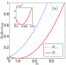
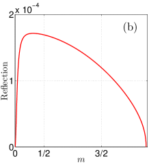
Figure 9: (Color online) Reflection probabilities as a function of the angular momentum projection $m$. The energy of incoming (outgoing) electron is $E_{F}=1$eV($E_{F}-V_{0}=-1$eV). The panel (a) displays the direct reflection probabilities: $R_{--}=|r^{m,-1}_{m,-1}|^{2}$ (solid, red) and $R_{++}=|r^{m,+1}_{m,+1}|^{2}$ (dashed, blue). The panel (b) displays the reflection probabilities with the spin-flip: $R_{-+}=|r^{m,-1}_{m,+1}|^{2}=|r^{m,+1}_{m,-1}|^{2}$. The parameters are the same as in Fig.2.

The reflection probabilities for different $m$ are displayed on Fig.9. The direct reflection (without the spin-flip) grows rapidly with the increase of the magnetic quantum number $m$ (see Fig.9a). In contrast, the spin-flip reflection probabilities tends to zero with the increase of the magnetic quantum number (see Fig.9b). In comparison with the case $\lambda_{y}=0$, the minimum in the reflection probability $|r^{m,-1}_{m,-1}|^{2}$ is slightly shifted from $m^{\prime}=1/2+2p\delta$ (see the insert in Fig.9a)). In contrast to the case with $\lambda_{y}=0$, the direct reflection probability $|r^{m,-1}_{m,-1}|^{2}$ can not be turned to zero by the Aharonov-Bohm magnetic flux alone, created by the magnetic field along the nanotube symmetry ($y$-) axis. The larger is the quantum number $m$ the smaller is the transmission probability.

The maximal magnetic quantum number $m$, which corresponds to a complete reflection, could be determined from the condition that the longitudinal current $\langle\hat{j}_{y}\rangle_{m,s}=0$ (see Appendix A). This condition requires $t_{y}=\gamma k_{y}=0$ after the potential step. Note that the quantum number $s$ is not conserved at $\lambda_{y}\neq 0$. As a result, one obtains with the aid of Eqs.(A.22) for the energy of outgoing electron the condition

$$t_{y}=0\Rightarrow|E_{F}-V_{0}|=E_{m,s}^{0}\equiv|E_{m,s}(k_{y}=0)|\,,$$ (91)

$$E_{m,s}(k_{y}=0)=\sqrt{t_{m}^{2}+\lambda_{y}^{2}}+s\lambda_{x}\,,\quad s=\pm 1\,.$$ (92)

At fixed parameters $\{E_{F},V_{0},\lambda_{x,y},R\}$, one defines the boundaries

$$C_{\pm}=t_{m}^{2}=\left(\frac{\gamma}{R}m\right)^{2}=(|E_{F}-V_{0}|\mp\lambda_{x})^{2}-\lambda_{y}^{2}.$$ (93)

Note that $C_{-}>C_{+}$, and, therefore, the maximal $m=M$ is determined as

$$M=\frac{R}{\gamma}\sqrt{C_{-}}\,.$$ (94)

For all $|m|\geq M$ the transmition probability $T_{s-}\equiv 0$ for $s=\pm 1$. In particular, for our choice of parameters the reflection probability $R_{--}=|r^{m,-1}_{m,-1}|^{2}=1$ at $M\approx 7/2$ (compare with Fig.9a).

From now on we can define the critical angle of the complete reflection. In virtue of results from Appendix A we obtain for the critical angle

$$\tan(\phi)=\frac{\langle j_{\theta}\rangle_{q}}{\langle j_{y}\rangle_{q}}=\frac{t_{M}}{t_{y}}\left(1+\frac{\lambda_{x}^{2}-\lambda_{y}^{2}}{W}\right),$$ (95)

$$W=\sqrt{\lambda_{y}^{2}E_{F}^{2}+t_{M}^{2}(\lambda_{x}^{2}-\lambda_{y}^{2})}\,,$$ (96)

where the critical value of the magnetic quantum number $m$ is related to the variable $t_{M}$

$$t_{M}=\sqrt{C_{-}}=\sqrt{(|E_{F}-V_{0}|+\lambda_{x})^{2}-\lambda_{y}^{2}}\,.$$ (97)

We use $s=+1$ in Eq.(95), since $t_{y}(s=+1)<t_{y}(s=-1)$, where $t_{y}$ is defined by Eq.(A.26)

$$t_{y}=\gamma k_{s}=\sqrt{E_{F}^{2}+\lambda_{y}^{2}-t_{M}^{2}-\lambda_{x}^{2}-2sW}\,.$$ (98)

These equations might provide some hint on the contribution of different SOC terms at experimental measurements of the critical angle.

V.2 Basic features of a quantum dot

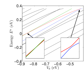
Figure 10: (Color online) The QD energy spectrum as a function of applied potential $V_{0}$. The levels with a quantum number $m=3/2$ are displayed for the nanotube with a length $L=100$Å. The other parameters are the same as in Fig.2. At different values of the applied potential, levels either cross (left insert) or repel (right insert) each other.

The energy spectrum of a QD is defined by the minimal gap for a given angular momentum $m$: $-E_{m,-1}^{0}<E^{n}_{m}<E_{m,-1}^{0}$. The mixing of spin components could lead to the interaction between spectra inherited from the ones with different spin projection (at $\lambda_{y}=0$). In particular, a crossing/anti-crossing behavior of two levels depends on their symmetry with respect to the inversion of the $y$-axis (see Fig.10). Two levels with the same parity $\Psi_{1,2}=s_{1,2}\hat{M}_{y}\Psi_{1,2}$ (when $s_{1}=s_{2}$) anti-cross, while a different sign $s_{1}=-s_{2}$ leads to the level crossing. Other properties of discrete levels are very similar to properties of those obtained at $\lambda_{y}=0$.

VI Summary

Within the approach suggested by Ando (see details in Ando ), we solved analytically the eigenvalue problem for the effective mass Hamiltonian for electrons on curved surface with the spin-orbit interaction. In particular, with the aid of transformation (7), we obtained explicit expressions for a low energy spectrum and eigenstates of armchair carbon nanotubes. These findings have been used to analyze transport properties of the CNT with the curvature-induced SOC (see Eq.(11)) at different limits.

We have studied effects produced by the SOC on the scattering of electrons at the interface introduced by the potential step of height $V_{0}$. The effect of the SOC becomes especially drastic when the height of the potential barrier can be controlled to reach conditions allowing to produce a spin-filter effect. At this condition only one spin component is dominant in the transmission over the CNT. Note that this phenomenon occurs due to the ”effective magnetic field” which is brought about by the curvature induced SOC. The SOC term $\lambda_{y}$ yields, however, a parasite loss $(\sim 10^{-3})$ of the spin-filter effect.

The gap in CNTs (due to the SOC) opens a possibility to create a nanotube quantum dot. In the limit of the preserved spin symmetry we have calculated the QD eigenstates with aid of the transcendental equation. At low energy limit the spectrum is similar to the one of the quantum well potential, while for large energies it carries features of the harmonic oscillator spectrum. In such QDs an electron with spin up cannot scatter into state with spin down and vise versa, without any additional mechanism. However, the SOC term $\lambda_{y}$ mixes these states and yields the anti-crossing effect. This mechanism may affect the spin relaxation phenomenon in the system under consideration, in addition to an electron-phonon coupling mechanism Loss .

There was a belief that the curvature induced SOC in graphene, restricted by the first term, leads only to very weak back scattering Ando . We have demonstrated, however, that the second term, ignored in a previous analysis, produces the inter-channel scattering, which could increase the back scattering by a few orders of magnitude and enrich transport phenomena in carbon nanotubes.

Appendix A An eigenvalue problem for $\hat{H}^{\prime}$

We suggest to use the eigenstate in the form

$$F^{\prime}(\theta,y)=e^{\mathrm{i}m\theta}e^{\mathrm{i}k_{y}y}\left(\begin{array}[]{c}A\\ B\\ C\\ D\end{array}\right),m=\pm 1/2,\pm 3/2,....$$ (A.1)

to solve the eigenvalue problem $\hat{H}^{\prime}F^{\prime}=EF^{\prime}$ for the Hamiltonian (8). As a result, one obtains the Hamiltonian (17). In virtue of the unitary transformation

$${\tilde{V}}=\hat{P}_{123}\hat{\tau}_{x}\otimes\exp\left(\mathrm{i}\frac{\pi}{4}\hat{\sigma}_{x}\right)=$$ (A.2)

$$\frac{1}{\sqrt{2}}\left(\begin{array}[]{cccc}0&0&1&0\\ 1&0&0&0\\ 0&1&0&0\\ 0&0&0&1\\ \end{array}\right)\left(\begin{array}[]{cccc}0&0&1&\mathrm{i}\\ 0&0&\mathrm{i}&1\\ 1&\mathrm{i}&0&0\\ \mathrm{i}&1&0&0\\ \end{array}\right)=\frac{1}{\sqrt{2}}\left(\begin{array}[]{cccc}1&\mathrm{i}&0&0\\ 0&0&1&\mathrm{i}\\ 0&0&\mathrm{i}&1\\ \mathrm{i}&1&0&0\\ \end{array}\right)$$ (A.15)

our Hamiltonian (17) becomes real

$$\hat{\tilde{H}}={\tilde{V}}^{-1}\hat{H}^{\prime}{\tilde{V}}=$$ (A.16)

$$\left(\begin{array}[]{cccc}-\lambda_{x}-\lambda_{y}&0&t_{y}&t_{m}\\ 0&\lambda_{x}+\lambda_{y}&t_{m}&-t_{y}\\ t_{y}&t_{m}&\lambda_{x}-\lambda_{y}&0\\ t_{m}&-t_{y}&0&-\lambda_{x}+\lambda_{y}\\ \end{array}\right)$$ (A.21)

with notations (23). The eigenvalues of the Hamiltonian (A.16) are

$$E=\pm E_{m,s}\,,$$ (A.22)

$$E_{m,s}=\sqrt{t_{m}^{2}+t_{y}^{2}+\lambda_{y}^{2}+\lambda_{x}^{2}+2D_{m,s}}\,,\quad s=\pm 1\,,$$

$$D_{m,s}=s\sqrt{\lambda_{x}^{2}\left(t_{m}^{2}+\lambda_{y}^{2}\right)+t_{y}^{2}\lambda_{y}^{2}}.$$

Eigenvectors have rather simple form

$${\cal V}_{m,s}=\frac{1}{N_{m,s}}\Bigg{(}\frac{-D_{m,s}+\lambda_{y}(E-\lambda_{y})}{t_{m}(\lambda_{x}+\lambda_{y})},$$ (A.23)

$$\frac{-t_{y}(\lambda_{x}-\lambda_{y})}{-D_{m,s}+\lambda_{x}(E-\lambda_{x})},\frac{t_{y}}{t_{m}}\frac{(-D_{m,s}+\lambda_{y}(E-\lambda_{y}))}{(-D_{m,s}+\lambda_{x}(E-\lambda_{x}))},1\Bigg{)}^{T},$$

where the values $E=\pm E_{m,s}$, $D_{m,s}$ are defined by Eqs.(A.22), and the norm $N_{m,s}$ is

$$\begin{array}[]{rcl}N_{m,s}&=&\sqrt{({\cal F}_{1}+{\cal F}_{2}+{\cal F}_{3})/{\cal M}+1},\\ {\cal F}_{1}&=&\left(D_{m,s}-\lambda_{y}(E-\lambda_{y})\right)^{2}\left(D_{m,s}-\lambda_{x}(E-\lambda_{x})\right)^{2},\\ {\cal F}_{2}&=&t_{m}^{2}t_{y}^{2}(\lambda_{x}^{2}-\lambda_{y}^{2})^{2},\\ {\cal F}_{3}&=&t_{y}^{2}(\lambda_{x}+\lambda_{y})^{2}\left(D_{m,s}-\lambda_{y}(E-\lambda_{y})\right)^{2},\\ {\cal M}&=&t_{m}^{2}(\lambda_{x}+\lambda_{y})^{2}(D_{m,s}-\lambda_{x}(E-\lambda_{x}))^{2}.\end{array}$$ (A.24)

The expectation value of the current for eigenspinors (A.23) could be calculated with the aid of the definitions (32) and the transformation (A.2). As a result, we obtain

$$\langle\hat{j}_{y}\rangle_{m,s}=\frac{\gamma t_{y}}{E}\left(1+\frac{\lambda_{y}^{2}}{D_{m,s}}\right),$$

$$\langle\hat{j}_{\theta}\rangle_{m,s}=\frac{\gamma t_{m}}{E}\left(1+\frac{\lambda_{x}^{2}}{D_{m,s}}\right).$$ (A.25)

To solve a scattering problem we need the eigenspinors for a fixed value of the energy $E$. Using the dispersion relation (A.22), we obtain

$$k_{m,s}=\frac{1}{\gamma}\sqrt{E^{2}+\lambda_{y}^{2}-t_{m}^{2}-\lambda_{x}^{2}-2s\sqrt{\lambda_{y}^{2}E^{2}+t_{m}^{2}(\lambda_{x}^{2}-\lambda_{y}^{2})}}\,.$$ (A.26)

Substituting the value of $k_{m,s}$ from Eq. (A.26), the spinor (A.23) becomes ${\cal V}_{m,s}(t_{y}=\gamma k_{m,s})$ with the parameter $D_{m,s}$ simplified to the form

$$D_{m,s}=s\sqrt{\lambda_{y}^{2}E^{2}+t_{m}^{2}(\lambda_{x}^{2}-\lambda_{y}^{2})}-\lambda_{y}^{2}.$$ (A.27)

References

- (1) R. Saito, G. Dresselhaus, and M.S. Dresselhaus, Physical Properties of Carbon Nanotubes (Imperial College Press, London, 1998).
- (2) T. Ando, J.Phys.Soc.Jap. 74 (2005) 777.
- (3) M.S. Dresselhaus, G. Dresselhaus, R. Saito, and A. Jorio, Phys. Rep. 409 (2005) 47.
- (4) J.-C. Charlier, X. Blase, and S. Roshe, Rev. Mod. Phys. 79 (2007) 677.
- (5) Q. Zhang, J-Qi Huang, W.-Z. Qian, Y.-Y. Zhang, and F. Wei, Small 8 (2013) 1237.
- (6) S. W. Lee and E.E.B. Campbell, Cur. App. Phys. 13 (2013) 1844.
- (7) H. Min, J. E. Hill, N. A. Sinitsyn, B. R. Sahu, L. Kleinman, and A. H. MacDonald, Phys. Rev. B 74 (2006) 165310.
- (8) A. H. Castro Neto, F. Guinea, N. M. R. Peres, K. S. Novoselov, and A. K. Geim, Rev. Mod. Phys. 81 (2009) 109.
- (9) C. L. Kane and E. J. Mele, Phys. Rev. Lett. 78 (1997) 1932.
- (10) P. Allain and J. Fuchs, Eur.Phys.J.B 83 (2011) 301.
- (11) T. Ando, J. Phys. Soc. Japan 69 (2000) 1757.
- (12) M.V. Entin and L.I. Magarill, Phys. Rev. B 64 (2001) 085330.
- (13) A. De Martino, R. Egger, K. Hallberg, and C.A. Balseiro, Phys. Rev. Lett. 88 (2002) 206402.
- (14) D. Huertas-Hernando, F. Guinea, and A. Brataas, Phys. Rev. B 74 (2006) 155426.
- (15) F. Kuemmeth, S.Ilani, D.C. Ralph, and P.L. McEuen, Nature 452 (2008) 448.
- (16) D.V. Bulaev, B. Trauzettel, and D. Loss, Phys. Rev. B 77 (2008) 235301.
- (17) L. Chico, M.P. López-Sancho, and M. C. Muñoz, Phys. Rev. B 79 (2009) 235423.
- (18) J.-S. Jeong and H.-W. Lee, Phys. Rev. B 80 (2009) 075409.
- (19) W. Izumida, K. Sato, and R. Saito, J. Phys. Soc. Jpn. 78 (2009) 074707.
- (20) M. del Valle, M. Magrańska, and M. Grifoni, Phys. Rev. B 84 (2011) 165427.
- (21) P. Středa and P.Šeba, Phys. Rev. Lett. 90 (2003) 256601.