Abstraction of Elementary Hybrid Systems by Variable Transformation

Abstract

Elementary hybrid systems (EHSs) are those hybrid systems (HSs) containing elementary functions such as exp, ln, sin, cos, etc. EHSs are very common in practice, especially in safety-critical domains. Due to the non-polynomial expressions which lead to undecidable arithmetic, verification of EHSs is very hard. Existing approaches based on partition of state space or over-approximation of reachable sets suffer from state explosion or inflation of numerical errors. In this paper, we propose a symbolic abstraction approach that reduces EHSs to polynomial hybrid systems (PHSs), by replacing all non-polynomial terms with newly introduced variables. Thus the verification of EHSs is reduced to the one of PHSs, enabling us to apply all the well-established verification techniques and tools for PHSs to EHSs. In this way, it is possible to avoid the limitations of many existing methods. We illustrate the abstraction approach and its application in safety verification of EHSs by several real world examples.

1 Introduction

Complex Embedded Systems (CESs) consist of software and hardware components that operate autonomous devices interacting with the physical environment. They are now part of our daily life and are used in many industrial sectors to carry out highly complex and often critical functions. The development process of CESs is widely recognized as a highly complex and challenging task. A thorough validation and verification activity is necessary to enhance the quality of CESs and, in particular, to fulfill the quality criteria mandated by the relevant standards. Hybrid systems (HSs) are mathematical models with precise mathematical semantics for CESs, wherein continuous physical dynamics are combined with discrete transitions. Based on HSs, rigorous analysis and verification of CESs become feasible, so that errors can be detected and corrected in the very early stage of design.

In practice, it is very common to model complex physical environments by ordinary differential equations (ODEs) with elementary functions such as reciprocal function $\frac{1}{x}$, exponential function $e^{x}$, logarithm function $\ln x$, trigonometric functions $\sin x$ and $\cos x$, and their compositions. We call such HSs elementary HSs (EHSs). As elementary expressions usually lead to undecidable arithmetic, the verification of EHSs becomes very hard, even intractable. Existing methods that deal with EHS verification include the level-set method [21], the hybridization method [3, 13], the gridding-based abstraction refinement method [27], the interval SMT solver-based method [7, 6], the Taylor model-based flowpipe approximation method [4], and so on. These methods rely either on iterative partition of state space or on iterative computation of approximate reachable sets, which can quickly lead to explosion of state numbers or inflation of numerical errors. Moreover, most of the above mentioned methods can only do bounded model checking (BMC).

As an alternative, the constraint-based approach verifies the safety property of a HS by solving corresponding constraints symbolically or numerically, to discover a barrier (inductive invariant) that separates the reachable set from the unsafe region, which avoids exhaustive gridding or brute-force computation, and can thus overcome the limitations of the above mentioned methods. However, this method has mainly been applied to verification of polynomial hybrid systems (PHSs) [31, 25, 24, 10, 18]. Although ideas about generating invariants for EHSs appeared in [24, 8], they were talked about in an ad hoc way. In [30], the author proposed a change-of-bases method to transform EHSs to PHSs, even to linear systems, but the success depends on the choice of the set of basis functions, and therefore does not apply to general EHSs.

In this paper, we investigate symbolic abstraction of general EHSs to PHSs, by extending [30] with early works on polynomilization of elementary ODEs [14, 32]. Herein the abstraction is accomplished by introducing new variables to replace the non-polynomial terms. With the substitution, flows, guards and other components of the EHSs are transformed according to the chain rule of differentiation, or by the over-approximation methods proposed in the paper, so that for any trajectory of the EHSs, there always exists a corresponding trajectory of the reduced PHSs. Besides, such abstraction preserves (inductive) invariant sets. Therefore, verification of the EHSs is naturally reduced to the one of the reduced PHSs. This will be shown by several real world verification problems.

The proposed abstraction applies to general EHSs. The benefit of the proposed abstraction is that it enables all the well-established verification techniques and tools for PHSs, especially the constraint-based approaches such as DAL [23] and SOS [25, 16], to be applied to EHSs, and thus provides the possibility of avoiding such limitations as error inflation, state explosion and boundedness for existing EHS verification methods. A by-product is that it also provides the possibility of generating invariants with elementary functions for PHSs, thus enhancing the power of existing PHS verification methods. In short, the proposed abstraction method can be a good alternative or complement to existing approaches.

Related Work.

This work is most closely related to [30] and [14]. The abstraction in this paper is performed by systematic augmentation of the original system rather than change-of-bases, thus essentially different from [30] and generally applicable. Compared to [14], this paper gives a clearer reduction procedure for elementary ODEs and discusses the extension to hybrid systems. This work is most closely related to [30] and [14]. The abstraction in this paper is performed by systematic augmentation of the original system rather than change-of-bases, thus essentially different from [30] and more general. Compared to [14], this paper gives a clearer reduction procedure for elementary ODEs and discusses the extension to hybrid systems. It was proved in [26] that safety verification of nonlinear hybrid systems is quasi-semidecidable, but to find efficient verification algorithms remains an open problem. An approximation technique for abstracting nonlinear hybrid systems to PHSs based on Taylor polynomial was proposed in [17], but to abstract the continuous flow transitions it requires the ODEs to have closed-form solutions. In [22], the authors adopted similar recasting techniques to ours for stability analysis of non-polynomial systems. Regarding non-polynomial invariants for polynomial continuous or hybrid systems, [28] presented the first method for generating transcendental invariants using formal power series, while the more recent work [9] proposed a Darboux Polynomial-based method. Both [28] and [9] can only find non-polynomial invariants of limited forms.

Paper Organization.

The rest of the paper is organized as follows. We briefly review some basic notions about hybrid systems and the theory of abstraction for hybrid systems in Section 2. Section 3 is devoted to the transformation from EDSs to PDSs, and from EHSs to PHSs. Section 4 discusses how to use the proposed abstraction approach for safety verification of EHSs. Section 5 concludes this paper.

2 Preliminary

In this section, we briefly introduce the basic knowledge of hybrid systems and define what we call elementary hybrid systems. Besides, we also recall the basic theory of abstraction for hybrid systems originally developed in [29, 30].

Throughout this paper, we use $\mathbb{N},\mathbb{Q},\mathbb{R}$ to denote the set of natural, rational and real numbers respectively. Given a set $A$, the power set of $A$ is denoted by $2^{A}$, and the Cartesian product of $n$ duplicates of $A$ is denoted by $A^{n}$; for instance, $\mathbb{R}^{n}$ stands for the $n$-dimensional Euclidean space. A vector element $(a_{1},a_{2},\ldots,a_{n})\in A^{n}$ is usually abbreviated by a boldface letter $\mathbf{a}$ when its dimension is clear from the context.

2.1 Elementary Continuous and Hybrid Systems

A continuous dynamical system (CDS) is modeled by first-order autonomous ordinary differential equations (ODEs)

$$\dot{\mathbf{x}}=\mathbf{f}(\mathbf{x}),$$ (1)

where $\mathbf{x}=(x_{1},\ldots,x_{n})\in\mathbb{R}^{n}$ and $\mathbf{f}:U\rightarrow\mathbb{R}^{n}$ is a vector function, called a vector field, defined on an open set $U\subseteq\mathbb{R}^{n}$. If $\mathbf{f}$ satisfies the local Lipschitz condition [15], then for any $\mathbf{x}_{0}\in U$, there exists a unique differentiable vector function $\mathbf{x}(t):(a,b)\rightarrow U$, where $(a,b)$ is an open interval containing $0$, such that $\mathbf{x}(0)=\mathbf{x}_{0}$ and the derivative of $\mathbf{x}(t)$ w.r.t. $t$ satisfies $\forall t\in(a,b).\,{\mathrm{d}\mathbf{x}(t)\over\mathrm{d}t}=\mathbf{f}(\mathbf{x}(t))$. Such $\mathbf{x}(t)$ is called the solution to (1) with initial value $\mathbf{x}_{0}$, or the trajectory of (1) starting from $\mathbf{x}_{0}$.

In many contexts, a CDS $\mathcal{C}$ may be equipped with an initial set $\Xi$ and a domain ${D}$, represented as a triple $\mathcal{C}\,\widehat{=}\,(\Xi,\mathbf{f},{D})$. If $\mathbf{f}$ is defined on $U\subseteq\mathbb{R}^{n}$, then $\Xi$ and $D$ should satisfy $\Xi\subseteq D\subseteq U$. In what follows, all CDSs will refer to the triple form unless otherwise stated. Hybrid systems (HSs) are those systems that exhibit both continuous evolutions and discrete transitions. A popular model of HSs is hybrid automata [1, 11].

Definition 1 (Hybrid Automaton)

A hybrid automaton (HA) is a system $\mathcal{H}\,\widehat{=}\,(Q,X,f,$ $D,E,G,R,\Xi)$,  where

• $Q=\{q_{1},\ldots,q_{m}\}$ is a finite set of modes;

• $X=\{x_{1},\ldots,x_{n}\}$ is a finite set of continuous state variables, with $\mathbf{x}=(x_{1},\ldots,x_{n})$ ranging over $\mathbb{R}^{n}$;

• $f:Q\rightarrow(U_{q}\rightarrow\mathbb{R}^{n})$ assigns to each mode $q\in Q$ a locally Lipschitz continuous vector field $\mathbf{f}_{q}$ defined on the open set $U_{q}\subseteq\mathbb{R}^{n}$;

• $D$ assigns to each mode $q\in Q$ a domain $D_{q}\subseteq U_{q}$;

• $E\subseteq Q\times Q$ is a finite set of discrete transitions;

• $G$ assigns to each transition $e\in E$ a guard $G_{e}\subseteq\mathbb{R}^{n}$;

• $R$ assigns to each transition $e\in E$ a set-valued reset function $R_{e}$: $G_{e}\rightarrow 2^{\mathbb{R}^{n}}$;

• $\Xi$ assigns to each $q\in Q$ a set of initial states $\Xi_{q}\subseteq D_{q}$.

Actually a HA can be regarded as a composition of a finite set of CDSs $\mathcal{C}_{q}\,\widehat{=}\,(\Xi_{q},\mathbf{f}_{q},$ $D_{q})$ for $q\in Q$, together with the set of transition relations specified by $(G_{e},R_{e})$ for $e\in E$. Conversely, any CDS can be regarded as a special HA with a single mode and without discrete transitions.

In this paper, we consider the class of HSs that can be defined by multivariate elementary functions given by the following grammar:

$$f,g ::= c\mid x\mid f+g\mid f-g\mid f\times g\mid$$ (3)

$$\frac{f}{g}\mid f^{a}\mid e^{f}\mid\ln(f)\mid\sin(f)\mid\cos(f)\enspace,$$

where $c\in\mathbb{R}$ is any real constant, $a\in\mathbb{Q}$ is any rational constant, and $x$ can be any variable from the set of real-valued variables $\{x_{1},\ldots$, $x_{n}\}$. In particular, the set of functions constructed only by (3) are multivariate polynomials in $x_{1},x_{2},\ldots,x_{n}$.

Definition 2 (Elementary and Polynomial HSs)

A HS or CDS is called elementary (resp. polynomial) if it can be expressed by elementary (resp. polynomial) functions together with relational symbols $\geqslant,>,\leqslant,<,=,\neq$ and Boolean connectives $\wedge,\vee,\neg,$ $\longrightarrow,\longleftrightarrow$.

Elementary (resp. polynomial) HSs or CDSs will be denoted by EHSs or EDSs (resp. PHSs or PDSs) for short.

Remark 1

The limitation of elementary functions to grammar (3) and (3) is not essential. For example, tangent and cotangent functions $\tan(f),\cot(f)$ can be easily defined. Besides, the presented approach in this paper is also applicable to other elementary functions not mentioned above, such as inverse trigonometric functions $\arcsin(f),$ $\arccos(f)$, etc. However, it does exclude functions like

$$f(x)=\left\{\begin{array}[]{ll}\frac{\sin x}{x}&\textrm{if $x\neq 0$}\\ \,\,\,\,\scriptstyle{1}&\textrm{if $x=0$}\\ \end{array}\right..$$

2.2 Semantics of Hybrid Systems

Given a HA $\mathcal{H}$, denote the state space of $\mathcal{H}$ by $\mathbb{H}\,\widehat{=}\,Q\times\mathbb{R}^{n}$, the domain of $\mathcal{H}$ by $D_{\mathcal{H}}\,\widehat{=}\,\bigcup_{q\in Q}(\{q\}\times{D}_{q})$, and the set of all initial states by $\Xi_{\mathcal{H}}\,\widehat{=}\,\bigcup_{q\in Q}(\{q\}\times\Xi_{q})$. The semantics of $\mathcal{H}$ can be characterized by the set of reachable states of $\mathcal{H}$.

Definition 3 (Reachable Set)

Given a HA $\mathcal{H}$, the reachable set of $\mathcal{H}$, denoted by $\mathcal{R}_{\mathcal{H}}$, consists of such $(q,\mathbf{x})\in\mathbb{H}$  for which there exists a finite sequence

$$(q_{0},\mathbf{x}_{0}),(q_{1},\mathbf{x}_{1}),\ldots,(q_{l},\mathbf{x}_{l})$$

such that $(q_{0},\mathbf{x}_{0})\in\Xi_{\mathcal{H}}$, $(q_{l},\mathbf{x}_{l})=(q,\mathbf{x})$, and for any $0\leqslant i\leqslant l-1$, one of the following two conditions holds:

• (Discrete Jump): $e=(q_{i},q_{i+1})\in E$,  $\mathbf{x}_{i}\in G_{e}$ and $\mathbf{x}_{i+1}\in R_{e}(\mathbf{x}_{i})$; or

• (Continuous Evolution): $q_{i}=q_{i+1}$, and there exists a $\delta\geqslant 0$ s.t. the trajectory $\mathbf{x}(t)$ of $\dot{\mathbf{x}}=\mathbf{f}_{q_{i}}$ starting from $\mathbf{x}_{i}$ satisfies

  • $\mathbf{x}(t)\in D_{q_{i}}$ for all $t\in[0,\delta]$; and

  • $\mathbf{x}(\delta)=\mathbf{x}_{i+1}$ .

Exact computation of reachable sets of hybrid systems is generally an intractable problem. For verification of safety properties, appropriate over-approximations of reachable sets will suffice.

Definition 4 (Invariant)

Given a HA $\mathcal{H}$, a set $\mathcal{I}\,\widehat{=}\,\bigcup_{q\in Q}(\{q\}\times I_{q})\subseteq\mathbb{H}$ is called an invariant of $\mathcal{H}$, if $\mathcal{I}$ is a superset of the reachable set $\mathcal{R}_{\mathcal{H}}$, i.e. $\mathcal{R}_{\mathcal{H}}\subseteq\mathcal{I}$.

Definition 5 (Inductive Invariant)

Given a HA $\mathcal{H}$, a set $\mathcal{I}\,\widehat{=}\,\bigcup_{q\in Q}(\{q\}\times I_{q})\subseteq\mathbb{H}$ is called an inductive invariant of $\mathcal{H}$, if $\mathcal{I}$ satisfies the following conditions:

• $\Xi_{q}\subseteq I_{q}$ for all $q\in Q$;

• for any $e=(q,q^{\prime})\in E$, if $\mathbf{x}\in I_{q}\cap G_{e}$, then $R_{e}(\mathbf{x})\subseteq I_{q^{\prime}}$;

• for any $q\in Q$ and any $\mathbf{x}_{0}\in I_{q}$, if ${\mathbf{x}}(t)$ is the trajectory of $\dot{\mathbf{x}}=\mathbf{f}_{q}$ starting from $\mathbf{x}_{0}$, and there exists $T\geqslant 0$ s.t. ${\mathbf{x}}(t)\in D_{q}$ for all $t\in[0,T]$, then ${\mathbf{x}}(T)\in I_{q}$ .

It is easy to check that any inductive invariant is also an invariant.

2.3 Abstraction of Hybrid Systems

We next briefly introduce the kind of abstraction for HSs proposed in [29, 30] and the significant properties about such abstraction.

In what follows, to distinguish between the dimensions of a HS and its abstraction, we will annotate a HS $\mathcal{H}$ (a CDS $\mathcal{C}$) with the vector of its continuous state variables $\mathbf{x}$ as $\mathcal{H}_{\mathbf{x}}$ ($\mathcal{C}_{\mathbf{x}}$). We use $|\mathbf{x}|$ to denote the dimension of $\mathbf{x}$. Given a vector function $\Theta$ that maps from $D\subseteq\mathbb{R}^{|\mathbf{x}|}$ to $\mathbb{R}^{|\mathbf{y}|}$, let $\Theta(A)\,\widehat{=}\,\{\Theta(\mathbf{x})\mid\mathbf{x}\in A\}$ for any $A\subseteq D$, and $\Theta^{-1}(B)\,\widehat{=}\,\{\mathbf{x}\in D\mid\Theta(\mathbf{x})\in B\}$ for any $B\subseteq\mathbb{R}^{|\mathbf{y}|}$.

Definition 6 (Simulation [29])

Given two CDSs $\mathcal{C}_{\mathbf{x}}\,\widehat{=}\,$ $(\Xi_{\mathbf{x}},\mathbf{f}_{\mathbf{x}},D_{\mathbf{x}})$ and $\mathcal{C}_{\mathbf{y}}\,\widehat{=}\,(\Xi_{\mathbf{y}},\mathbf{f}_{\mathbf{y}},$ $D_{\mathbf{y}})$, we say $\mathcal{C}_{\mathbf{y}}$ simulates $\mathcal{C}_{\mathbf{x}}$ or $\mathcal{C}_{\mathbf{x}}$ is simulated by $\mathcal{C}_{\mathbf{y}}$ via a continuously differentiable mapping $\Theta:D_{\mathbf{x}}\rightarrow\mathbb{R}^{|\mathbf{y}|}$, if $\Theta$ satisfies

• $\Theta(\Xi_{\mathbf{x}})\subseteq\Xi_{\mathbf{y}}$, $\Theta(D_{\mathbf{x}})\subseteq D_{\mathbf{y}}$; and

• for any trajectory $\mathbf{x}(t)$ of $\mathcal{C}_{\mathbf{x}}$ (i.e. a trajectory of $\dot{\mathbf{x}}=\mathbf{f}_{\mathbf{x}}(\mathbf{x})$ that starts from $\Xi_{\mathbf{x}}$ and stays in $D_{\mathbf{x}}$),  $\Theta\circ\mathbf{x}(t)$ is a trajectory of $\mathcal{C}_{\mathbf{y}}$, where $\circ$ denotes composition of functions.

We call $\mathcal{C}_{\mathbf{y}}$ an abstraction of $\mathcal{C}_{\mathbf{x}}$ under the simulation map $\Theta$.

Abstraction of a HS can be obtained by abstracting the CDS corresponding to each mode using an individual simulation map. As argued in [30], it can be assumed without loss of generality that the collection of simulation maps for each mode all map to an Euclidean space of the same dimension, say $\mathbb{R}^{|\mathbf{y}|}$.

Definition 7 (Simulation [30])

Given two HSs $\mathcal{H}_{\mathbf{x}}\,\widehat{=}\,(Q,X,f_{\mathbf{x}},D_{\mathbf{x}},E,G_{\mathbf{x}},R_{\mathbf{x}},\Xi_{\mathbf{x}})$ and $\mathcal{H}_{\mathbf{y}}\,\widehat{=}\,(Q,Y,f_{\mathbf{y}},D_{\mathbf{y}},E,G_{\mathbf{y}},$ $R_{\mathbf{y}},\Xi_{\mathbf{y}})$, we say $\mathcal{H}_{\mathbf{y}}$ simulates $\mathcal{H}_{\mathbf{x}}$ via the set of maps $\{\Theta_{q}:D_{\mathbf{x},q}\rightarrow\mathbb{R}^{|\mathbf{y}|}\mid q\in Q\}$, if the following hold:

• $(\Xi_{{\mathbf{y}},q},\mathbf{f}_{{\mathbf{y}},q},D_{{\mathbf{y}},q})$ simulates $(\Xi_{{\mathbf{x}},q},\mathbf{f}_{{\mathbf{x}},q},D_{{\mathbf{x}},q})$ via $\Theta_{q}$, for each $q\in Q$;

• $\Theta_{q}(G_{{\mathbf{x}},e})\subseteq G_{{\mathbf{y}},e}$, for any $e=(q,q^{\prime})\in E$;

• $\Theta_{q^{\prime}}(R_{{\mathbf{x}},e}({\mathbf{x}}))\subseteq R_{{\mathbf{y}},e}(\Theta_{q}({\mathbf{x}}))$, for any $e=(q,q^{\prime})\in E$ and any ${\mathbf{x}}\in G_{\mathbf{x},e}$.

We call $\mathcal{H}_{\mathbf{y}}$ an abstraction of $\mathcal{H}_{\mathbf{x}}$ under the set of simulation maps $\{\Theta_{q}\mid q\in Q\}$.

Intuitively, if $\mathcal{H}_{\mathbf{y}}$ is an abstraction of $\mathcal{H}_{\mathbf{x}}$, then for any $(q,\mathbf{x})$ reachable by $\mathcal{H}_{\mathbf{x}}$, $(q,\Theta_{q}(\mathbf{x}))$ is a state reachable by $\mathcal{H}_{\mathbf{y}}$. Actually, we can prove the following nice property about such abstractions.

Theorem 2.1 (Invariant Preserving Property)

If $\mathcal{H}_{\mathbf{y}}$ is an abstraction of $\mathcal{H}_{\mathbf{x}}$ under simulation maps $\{\Theta_{q}\mid q\in Q\}$, and $\mathcal{I}_{\mathbf{y}}\,\widehat{=}\,\bigcup_{q\in Q}(\{q\}\times I_{\mathbf{y},q})$ is an invariant (resp. inductive invariant) of $\mathcal{H}_{\mathbf{y}}$, then $\mathcal{I}_{\mathbf{x}}\,\widehat{=}\,\bigcup_{q\in Q}(\{q\}\times I_{\mathbf{x},q})$ with $I_{\mathbf{x},q}\,\widehat{=}\,\Theta_{q}^{-1}(I_{\mathbf{y},q})$ is an invariant (resp. inductive invariant) of $\mathcal{H}_{\mathbf{x}}$.

Theorem 2.1 extends Theorem 3.2 of [29] in two aspects: firstly, it deals with HSs, and secondly, it applies to both invariants and inductive invariants; nevertheless, the proof of Theorem 2.1 can be given in a similar way and so is omitted here. The significance of Theorem 2.1 lies in the possibility of analyzing a complex HS by analyzing certain abstractions of it, which may be of simpler forms and thus allow the use of any available techniques and tools.

The following theorem proposed in [29] is very useful for checking or constructing simulation maps.

Theorem 2.2 (Simulation Checking [29])

Let $\mathcal{C}_{\mathbf{x}}$, $\mathcal{C}_{\mathbf{y}}$, $\Theta$ be specified as in Definition 6. Suppose $|\mathbf{x}|=n,|\mathbf{y}|=\ell$, and $\Theta\,\widehat{=}\,(\theta_{1},\theta_{2},\ldots,\theta_{\ell})$. Then $\mathcal{C}_{\mathbf{y}}$ simulates $\mathcal{C}_{\mathbf{x}}$ if

• $\Theta(\Xi_{\mathbf{x}})\subseteq\Xi_{\mathbf{y}}$, $\Theta(D_{\mathbf{x}})\subseteq D_{\mathbf{y}}$; and

• $\mathbf{f}_{\mathbf{y}}(\Theta(\mathbf{x}))=\mathcal{J}_{\Theta}(\mathbf{x})\cdot\mathbf{f}_{\mathbf{x}}(\mathbf{x})$, for any $\mathbf{x}\in D_{\mathbf{x}}$, where $\mathbf{f}_{\mathbf{x}}(\mathbf{x})$ is seen as a column vector, and $\mathcal{J}_{\Theta}(\mathbf{x})$ represents the Jacobian matrix of $\Theta$ at point $\mathbf{x}$, i.e.

  $$\mathcal{J}_{\Theta}(\mathbf{x})=\left(\begin{array}[]{ccc}\frac{\partial{\theta_{1}}}{\partial x_{1}}&\ldots&\frac{\partial{\theta_{1}}}{\partial x_{n}}\\ \vdots&\ddots&\vdots\\ \frac{\partial{\theta_{\ell}}}{\partial x_{1}}&\ldots&\frac{\partial{\theta_{\ell}}}{\partial x_{n}}\\ \end{array}\right)\enspace.$$

We will employ this theorem to prove the correctness of our abstraction of EHSs in the following section.

3 Polynomial Abstraction of EHSs

In this section, given any EHS as defined in Definition 2, we will construct a PHS that simulates the EHS in the sense of Definition 7. The process of constructing such an abstraction can be divided into three steps: firstly, elementary ODEs can be transformed into polynomial forms by introducing new variables to replace non-polynomial terms occurring in the vector field functions; secondly, using the replacement relations, initial sets and domains, and thus EDSs, can be abstracted into polynomial forms; finally, discrete transitions, i.e. guards and reset functions, can be abstracted accordingly, which results in polynomial abstractions of EHSs.

3.1 Polynomialization of Elementary ODEs

In this part, we illustrate how to transform an elementary ODE $\dot{\mathbf{x}}=\mathbf{f}(\mathbf{x})$ equivalently into a polynomial one. The basic idea is to introduce a fresh variable $v$ for each non-polynomial term $\gamma(\mathbf{x})$ in $\mathbf{f}(\mathbf{x})$ and then substitute $v$ for $\gamma(\mathbf{x})$ in $\mathbf{f}(\mathbf{x})$; meanwhile differentiate the two sides of the replacement equation $v=\gamma(\mathbf{x})$ w.r.t. time and obtain a new ODE $\dot{v}=\nabla\gamma(\mathbf{x})\cdot\mathbf{f}(\mathbf{x})$, where $\nabla\gamma(\mathbf{x})$ denotes the gradient row vector of $\gamma(\mathbf{x})$; then append the new ODE to the original one (with $\gamma(\mathbf{x})$ replaced by $v$), and continue the above procedure to replace non-polynomial terms that may exist in $\nabla\gamma(\mathbf{x})$; finally when such a process terminates, a polynomial ODE together with a collection of replacement equations will be obtained. Note that the transformed polynomial ODE will always have a higher dimension than the original one.

Remark 2

Recasting elementary ODEs as polynomial ones has been proposed in early works in the field of physics and biosciences such as [14, 32] in order to obtain explicit solutions of EDSs. In this paper, we employ such an idea for formal verification and invariant generation for EHSs. The basic transformation here is similar to [14], but we give a clearer statement of the transformation procedure and extend it from ODEs to hybrid systems.

We next demonstrate the above idea on concrete examples.

3.1.1 Univariate Basic Elementary Functions

For

$$\dot{x}=f(x)$$ (4)

• if $f(x)=\frac{1}{x}$, then let $v=\frac{1}{x}$, and thus $\dot{v}=-\frac{\dot{x}}{x^{2}}$. Therefore (4) is transformed to

  $$\left\{\begin{array}[]{lll}\dot{x}&=&v\\ \dot{v}&=&-v^{3}\\ \end{array}\right.\enspace;$$

• if $f(x)=\sqrt{x}$, then let $v=\sqrt{x}$, and thus $\dot{v}=\frac{\dot{x}}{2\sqrt{x}}$. Therefore (4) is transformed to

  $$\left\{\begin{array}[]{lll}\dot{x}&=&v\\ \dot{v}&=&\frac{1}{2}\\ \end{array}\right.\enspace;$$

• if $f(x)=e^{x}$, then let $v=e^{x}$, and thus $\dot{v}=e^{x}\cdot\dot{x}$. Therefore (4) is transformed to

  $$\left\{\begin{array}[]{lll}\dot{x}&=&v\\ \dot{v}&=&v^{2}\\ \end{array}\right.\enspace;$$

• if $f(x)=\ln{x}$, then let $v=\ln{x}$, and thus $\dot{v}=\frac{\dot{x}}{x}$; then further let $u=\frac{1}{x}$, and thus $\dot{u}=-\frac{\dot{x}}{x^{2}}$. Therefore (4) is transformed to

  $$\left\{\begin{array}[]{lll}\dot{x}&=&v\\ \dot{v}&=&uv\\ \dot{u}&=&-u^{2}v\end{array}\right.\enspace;$$

• if $f(x)=\sin{x}$, then let $v=\sin{x}$, and thus $\dot{v}=\dot{x}\cdot\cos{x}$; then further let $u=\cos{x}$, and thus $\dot{u}=-\sin{x}\cdot\dot{x}$. Therefore (4) is transformed to

  $$\left\{\begin{array}[]{lll}\dot{x}&=&v\\ \dot{v}&=&uv\\ \dot{u}&=&-v^{2}\end{array}\right.\enspace;$$

• if $f(x)=\cos{x}$, then the transformation is analogous to the case of $f(x)=\sin{x}$.

3.1.2 Compositional and Multivariate Functions

Obviously, the outmost form of any compositional elementary function must be one of $f\pm g,f\times g,\frac{f}{g},f^{a},e^{f},\ln(f),\sin(f),\cos(f)$. Therefore given a compositional function, we can iterate the above procedure discussed on basic cases from the innermost non-polynomial sub-term to the outside, until all the sub-expressions have been transformed into polynomials. For example,

• if $f(x)=\ln({2+\sin{x}})$, we can let

  $$\left\{\begin{array}[]{ll}v&=\sin{x}\\ u&=\cos{x}\\ w&=\ln{(2+v)}=\ln{(2+\sin{x})}\\ z&=\frac{1}{2+v}=\frac{1}{2+\sin{x}}\\ \end{array}\right.\enspace,$$

and then (4) is transformed to

$$\left\{\begin{array}[]{lll}\dot{x}&=&w\\ \dot{v}&=&uw\\ \dot{u}&=&-vw\\ \dot{w}&=&zuw\\ \dot{z}&=&-z^{2}uw\end{array}\right.\enspace.$$

Handling multivariate functions is straightforward.

In summary, we give the following assertion on polynomializing elementary ODES, the correctness of which can be given based on the formal transformation algorithms presented in the appendix.

Proposition 1 (Polynomial Recasting)

Given an ODE $\dot{\mathbf{x}}=\mathbf{f}(\mathbf{x})$ with $\mathbf{f}(\mathbf{x})$ an elementary vector function defined on an open set $U\subseteq\mathbb{R}^{n}$, there exists a collection of variable replacement equations $\mathbf{v}=\Gamma(\mathbf{x})$, where $\mathbf{v}=(v_{1},v_{2},\ldots,v_{m})$ is a vector of new variables and $\Gamma(\mathbf{x})=(\gamma_{1}(\mathbf{x}),\gamma_{2}(\mathbf{x}),\ldots,\gamma_{m}(\mathbf{x})):U\rightarrow\mathbb{R}^{m}$ is an elementary vector function, such that

$${\left(\begin{array}[]{l}\dot{\mathbf{x}}\\ \dot{\mathbf{v}}\end{array}\right)}=\left(\begin{array}[]{c}\mathbf{f}(\mathbf{x})\\ \mathcal{J}_{\Gamma}(\mathbf{x})\cdot\mathbf{f}(\mathbf{x})\end{array}\right) = \left(\begin{array}[]{c}\mathbf{f}(\mathbf{x})\\ \mathcal{J}_{\Gamma}(\mathbf{x})\cdot\mathbf{f}(\mathbf{x})\end{array}\right){\Big{\llbracket}\mathbf{v}/\Gamma(\mathbf{x})\Big{\rrbracket}}$$ (11)

$$\widehat{=} \tilde{\mathbf{f}}(\mathbf{x},\mathbf{v})$$ (12)

becomes a polynomial ODE, that is, $\tilde{\mathbf{f}}(\mathbf{x},\mathbf{v})$ is a polynomial vector function in variables $\mathbf{x}$ and $\mathbf{v}$. Here expr$\llbracket\mathbf{v}/\Gamma(\mathbf{x})\rrbracket$ means replacing any occurrence of the non-polynomial term $\gamma_{i}(\mathbf{x})$ in the expression expr by the corresponding variable $v_{i}$, for all $1\leqslant i\leqslant m$.

It can be proved that the number of variables $\mathbf{v}$ is at most triple the number of nonpolynomial terms in the original ODE, which can be a small number in practice. The transformed polynomial ODE as specified in Proposition 1 is equivalent to the original one in the following sense.

Theorem 3.1 (Trajectory Equivalence)

Let $\mathbf{f}(\mathbf{x})$, $\Gamma(\mathbf{x})$ and $\tilde{\mathbf{f}}(\mathbf{x},\mathbf{v})$ be as specified in Proposition 1. Then for any trajectory $\mathbf{x}(t)$ of $\dot{\mathbf{x}}=\mathbf{f}(\mathbf{x})$ starting from $\mathbf{x}_{0}\in U\subseteq\mathbb{R}^{n}$, $\big{(}\mathbf{x}(t),\Gamma(\mathbf{x}(t))\big{)}$ is the trajectory of $(\dot{\mathbf{x}},\dot{\mathbf{v}})=\tilde{\mathbf{f}}(\mathbf{x},\mathbf{v})$ starting from $(\mathbf{x}_{0},\Gamma(\mathbf{x}_{0}))$; conversely, for any trajectory $(\mathbf{x}(t),\mathbf{v}(t))$ of $(\dot{\mathbf{x}},\dot{\mathbf{v}})=\tilde{\mathbf{f}}(\mathbf{x},\mathbf{v})$ starting from $(\mathbf{x}_{0},\mathbf{v}_{0})\in\mathbb{R}^{n+m}$, if $\mathbf{x}_{0}\in U$ and $\mathbf{v}_{0}=\Gamma(\mathbf{x}_{0})$, then $\mathbf{x}(t)$ is the trajectory of $\dot{\mathbf{x}}=\mathbf{f}(\mathbf{x})$ starting from $\mathbf{x}_{0}$.

Proof

The result can be deduced directly from (12). ∎

3.2 Abstracting EDSs by PDSs

In this part, given an EDS $\mathcal{C}_{\mathbf{x}}\,\widehat{=}\,(\Xi_{\mathbf{x}},\mathbf{f}_{\mathbf{x}},D_{\mathbf{x}})$ we will construct a PDS $C_{\mathbf{y}}\,\widehat{=}\,(\Xi_{\mathbf{y}},\mathbf{f}_{\mathbf{y}},D_{\mathbf{y}})$ that simulates $\mathcal{C}_{\mathbf{x}}$. The construction is based on the procedure introduced in Section 3.1 on polynomial transformation of elementary ODEs. The basic idea is to construct a simulation map using the replacement equations. The difference here is that when abstracting an EDS, we need to replace non-polynomial terms occurring in not only the vector field, but also the initial set and domain. Roughly, the construction of $\mathcal{C}_{\mathbf{y}}$ consists of the following four steps.

1. Introduce new variables to replace all non-polynomial terms in $\mathbf{f}_{\mathbf{x}}$, $\Xi_{\mathbf{x}}$ and $D_{\mathbf{x}}$, and obtain a collection of replacement equations $\mathbf{v}=\Gamma(\mathbf{x})$ such that $\mathbf{f}_{\mathbf{x}}\llbracket\mathbf{v}/\Gamma(\mathbf{x})\rrbracket$, $\Xi_{\mathbf{x}}\llbracket\mathbf{v}/\Gamma(\mathbf{x})\rrbracket$ and $D_{\mathbf{x}}\llbracket\mathbf{v}/\Gamma(\mathbf{x})\rrbracket$ all become polynomial expressions.

2. Differentiate both sides of $\mathbf{v}=\Gamma(\mathbf{x})$ w.r.t. time to get $\dot{\mathbf{v}}=J_{\Gamma}(\mathbf{x})\cdot\mathbf{f}(\mathbf{x})$, and replace all newly appearing non-polynomial terms by introducing more variables.

3. Repeat (S2) until no more variables need to be introduced. For simplicity, still denote the final set of replacement equations by $\mathbf{v}=\Gamma(\mathbf{x})$. By Proposition 1, a polynomial vector field $\tilde{\mathbf{f}}(\mathbf{x},\mathbf{v})$ as in (12) will be obtained. Let $\mathbf{y}\,\widehat{=}\,(\mathbf{x},\mathbf{v})$ and define

   $$\mathbf{f}_{\mathbf{y}}(\mathbf{x},\mathbf{v})\quad\widehat{=}\quad\tilde{\mathbf{f}}(\mathbf{x},\mathbf{v})\enspace.$$ (13)

4. Define the simulation map $\Theta:D_{\mathbf{x}}\rightarrow\mathbb{R}^{|\mathbf{y}|}$ as

   $$\Theta(\mathbf{x})=(\mathbf{x},\Gamma(\mathbf{x}))\enspace.$$ (14)

   Then use $\Theta$ to construct $\Xi_{\mathbf{y}}$ and $D_{\mathbf{y}}$ as illustrated later.

After the above four steps, a CDS $(\Xi_{\mathbf{y}},\mathbf{f}_{\mathbf{y}},D_{\mathbf{y}})$ will be obtained, which is intended to be the polynomial abstraction of $\mathcal{C}_{\mathbf{x}}$ under simulation map $\Theta$. We next show how to get $\Xi_{\mathbf{y}}$ and $D_{\mathbf{y}}$ in detail to complete the construction.

The image of $\Xi_{\mathbf{x}}$ under the simulation map $\Theta$ is

$$\Theta(\Xi_{\mathbf{x}})=\{(\mathbf{x},\mathbf{v})\in\mathbb{R}^{|\mathbf{y}|}\mid\mathbf{x}\in\Xi_{\mathbf{x}}\wedge\mathbf{v}=\Gamma(\mathbf{x})\}\,,$$

briefly denoted by $\Theta(\Xi_{\mathbf{x}})\,\,\,\widehat{=}\,\,\,\Xi_{\mathbf{x}}\wedge\mathbf{v}=\Gamma(\mathbf{x})$, or alternatively

$$\Theta(\Xi_{\mathbf{x}})\,\,\,\widehat{=}\,\,\,\Xi_{\mathbf{x}}\llbracket\mathbf{v}/\Gamma(\mathbf{x})\rrbracket\wedge\mathbf{v}=\Gamma(\mathbf{x})\,.$$ (15)

By (S1), the first conjunct in (15) is of polynomial form, but the second conjunct contains elementary functions. By Definition 6, we need to get a polynomial over-approximation $\Xi_{\mathbf{y}}$ of $\Theta(\Xi_{\mathbf{x}})$, which means we need to abstract $\mathbf{v}=\Gamma(\mathbf{x})$ in (15) by polynomial expressions. We propose the following four ways to do so.

• When $\Gamma(\mathbf{x})$ are some special kinds elmentary functions, $\mathbf{v}=\Gamma(\mathbf{x})$ can be equivalently transformed to polynomial expressions, e.g.

  $$\left\{\begin{aligned} &v=\frac{1}{x}\Longleftrightarrow vx=1\\ &v=\sqrt{x}\Longleftrightarrow v^{2}=x\,\wedge\,v\geqslant 0\\ \end{aligned}\right.\enspace.$$ (16)

• If $\Xi_{\mathbf{x}}$ is a bounded region and the upper/lower bounds of each component $x_{i}$ of $\mathbf{x}$ can be easily obtained, then we can compute the Taylor polynomial expansion $\mathbf{p}(\mathbf{x})$ of $\Gamma(\mathbf{x})$ over the bounded region up to a certain degree, as well as an interval over-approximation $\mathbf{I}$ of the corresponding truncation error, such that $\mathbf{v}=\Gamma(\mathbf{x})$ can be approximated by $\mathbf{v}\in(\mathbf{p}(\mathbf{x})+\mathbf{I})$. We will illustrate this by an example presented later.

• We can also just compute the range of $\Gamma(\mathbf{x})$ (over $\Xi_{\mathbf{x}}$) as an over-approximation of $\mathbf{v}$, e.g.

  $$\left\{\begin{aligned} &v=\sin{x}\Longrightarrow-1\leqslant v\leqslant 1\\ &v=e^{x}\Longrightarrow v>0\\ \end{aligned}\right.\enspace.$$ (17)

• The simplest way is to remove the constraint $\mathbf{v}=\Gamma(\mathbf{x})$ entirely, which means $\mathbf{v}$ is allowed to take any value from $\mathbb{R}^{|\mathbf{v}|}$.

From (W1) to (W4), the over-approximation of $\mathbf{v}=\Gamma(\mathbf{x})$ becomes more and more coarse. Usually it takes more effort to obtain a more refined abstraction, but the result would be more helpful for analysis of the original system. We will discuss in Section 4 how to choose among (W1)-(W4) when constructing abstractions of EHSs, depending on what kind of inductive invariants are to be generated for safety verification tasks.

The construction of $D_{\mathbf{y}}$ is the same as $\Xi_{\mathbf{y}}$. Then we can give the following conclusion.

Theorem 3.2 (Abstracting EDS by PDS)

Given an EDS $\mathcal{C}_{\mathbf{x}}\,\widehat{=}\,(\Xi_{\mathbf{x}},\mathbf{f}_{\mathbf{x}},D_{\mathbf{x}})$, let $\mathcal{C}_{\mathbf{y}}\,\widehat{=}\,(\Xi_{\mathbf{y}},$ $\mathbf{f}_{\mathbf{y}},D_{\mathbf{y}})$, where $\mathbf{f}_{\mathbf{y}}$ is given by (13) and (12), and $\Xi_{\mathbf{y}},D_{\mathbf{y}}$ are given by (8) together with (W1)-(W4). Then $\mathcal{C}_{\mathbf{y}}$ is a polynomial abstraction of $\mathcal{C}_{\mathbf{x}}$ in the sense of Definition 6, under simulation map $\Theta$ defined by (14).

Proof

First, it is easy to check that $\mathcal{C}_{\mathbf{y}}$ is a PDS and $\Theta(\Xi_{\mathbf{x}})\subseteq\Xi_{\mathbf{y}}$, $\Theta(D_{\mathbf{x}})\subseteq D_{\mathbf{y}}$. Second, by (14) we have

$$\mathcal{J}_{\Theta}(\mathbf{x})=\left(\begin{array}[]{c}\mathbf{Id}_{|\mathbf{x}|}\\ \mathcal{J}_{\Gamma}(\mathbf{x})\end{array}\right)\enspace,$$

where $\mathbf{Id}_{|\mathbf{x}|}$ denotes the $|\mathbf{x}|$-dimensional identity matrix. Then for any $\mathbf{x}\in D_{\mathbf{x}}$,

$$\mathcal{J}_{\Theta}(\mathbf{x})\cdot\mathbf{f}_{\mathbf{x}}(\mathbf{x})=\left(\begin{array}[]{c}\mathbf{Id}_{|\mathbf{x}|}\\ \mathcal{J}_{\Gamma}(\mathbf{x})\end{array}\right)\cdot\mathbf{f}_{\mathbf{x}}(\mathbf{x})=\left(\begin{array}[]{c}\mathbf{f}_{\mathbf{x}}(\mathbf{x})\\ \mathcal{J}_{\Gamma}(\mathbf{x})\cdot\mathbf{f}_{\mathbf{x}}(\mathbf{x})\end{array}\right)\enspace.$$

Then according to the above formula and (14), (13) and (12), we get $\mathbf{f}_{\mathbf{y}}(\Theta(\mathbf{x}))=\mathbf{f}_{\mathbf{y}}(\mathbf{x},\Gamma(\mathbf{x}))=\tilde{\mathbf{f}}(\mathbf{x},\Gamma(\mathbf{x}))=\mathcal{J}_{\Theta}(\mathbf{x})\cdot\mathbf{f}_{\mathbf{x}}(\mathbf{x})$. Therefore by Theorem 2.2 we get the conclusion. ∎

Example 1

Consider the EDS $\mathcal{C}_{\mathbf{x}}\,\widehat{=}\,(\Xi_{\mathbf{x}},\mathbf{f}_{\mathbf{x}},D_{\mathbf{x}})$, where

• $\Xi_{\mathbf{x}}\,\widehat{=}\,(x+0.5)^{2}+(y-0.5)^{2}-0.16\leqslant 0$;

• $D_{\mathbf{x}}\,\widehat{=}\,-2\leqslant x\leqslant 2\wedge-2\leqslant y\leqslant 2$; and

• $\mathbf{f}_{\mathbf{x}}$ defines the ODE

  $$\left(\begin{array}[]{c}\dot{x}\\ \dot{y}\end{array}\right)=\left(\begin{array}[]{c}e^{-x}+y-1\\ -\sin^{2}(x)\end{array}\right)\enspace.$$ (18)

We will show how to construct a PDS $\mathcal{C}_{\mathbf{y}}$ that simulates $\mathcal{C}_{\mathbf{x}}$ following the above described steps.

• (S1-S3): Noticing that $\Xi_{\mathbf{x}}$ and $D_{\mathbf{x}}$ are both in polynomial forms, we only need to replace non-polynomial terms in $\mathbf{f}_{\mathbf{x}}$. We finally obtain the replacement relations $\mathbf{v}=\Gamma(\mathbf{x})$ given by

  $$(v_{1},v_{2},v_{3})=(\sin{x},e^{-x},\cos x)$$ (19)

  and the transformed polynomial ODE

  $$\left(\begin{array}[]{c}\dot{x}\\ \dot{y}\\ \dot{v}_{1}\\ \dot{v}_{2}\\ \dot{v}_{3}\end{array}\right)=\left(\begin{array}[]{c}v_{2}+y-1\\ -v_{1}^{2}\\ v_{3}(v_{2}+y-1)\\ -v_{2}(v_{2}+y-1)\\ -v_{1}(v_{2}+y-1)\end{array}\right)\enspace,$$ (20)

  the right-hand-side of which is defined to be $\mathbf{f}_{\mathbf{y}}$.

• (S4): The simulation map $\Theta$ is given by

  $$\Theta(x,y)=(x,y,\sin{x},e^{-x},\cos x)\enspace.$$

  The images of $\Xi_{\mathbf{x}}$ and $D_{\mathbf{x}}$ under $\Theta$ are

  $$\Theta(\Xi_{\mathbf{x}})\,\,\widehat{=}\,\,\Xi_{\mathbf{x}}\wedge v_{1}=\sin{x}\wedge v_{2}=e^{-x}\wedge v_{3}=\cos{x}$$

  and

  $$\Theta(D_{\mathbf{x}})\,\,\widehat{=}\,\,D_{\mathbf{x}}\wedge v_{1}=\sin{x}\wedge v_{2}=e^{-x}\wedge v_{3}=\cos{x}$$

  respectively. For the above two formulas, (W1) is not applicable, whereas we can use any of (W2)-(W4) to abstract them. Here we just give one possible way. First, use (W4) to abstract $\Theta(\Xi_{\mathbf{x}})$, and define $\Xi_{\mathbf{y}}\,\,\widehat{=}\,\,\Xi_{\mathbf{x}}$. Next, adopt (W2) to abstract $\Theta(D_{\mathbf{x}})$; using the tool COSY INFINITY for Taylor model [20] computation, we expand $\sin{x}$, $e^{-x}$ and $\cos{x}$ over $x\in[-2,2]$ at point $x=0$ up to degree 6, and obtain

  $$p_{1}(x)+l_{1}\leqslant v_{1}\leqslant p_{1}(x)+u_{1}$$ (21)

  $$\mathit{TM}_{\mathbf{x},\mathbf{v}}\,\widehat{=} \wedge p_{2}(x)+l_{2}\leqslant v_{2}\leqslant p_{2}(x)+u_{2}\enspace\enspace\enspace\enspace$$

  $$\wedge p_{3}(x)+l_{3}\leqslant v_{3}\leqslant p_{3}(x)+u_{3}\enspace.$$

  Figure 1 is an illustration of the relations between $v_{1},v_{2}$ and $x$ given by (21) and (• ‣ 3.2) respectively, where

  • $p_{1}(x)\,=\,2(0.5x)-1.333333333333333(0.5x)^{3}+0.2666666666666667(0.5x)^{5}$

  • $l_{1}=-0.08888888888890931$

  • $u_{1}=0.08888888888890931$

  and

  • $p_{2}(x)\,=\,1-2(0.5x)+2(0.5x)^{2}\,-1.333333333333333(0.5x)^{3}$

  • $+0.6666666666666666(0.5x)^{4}-0.2666666666666667(0.5x)^{5}$

  • $+0.08888888888888889(0.5x)^{6}$

  • $l_{2}=-0.1876585675919477$

  • $u_{2}=0.1876585675919477$  .

  

  

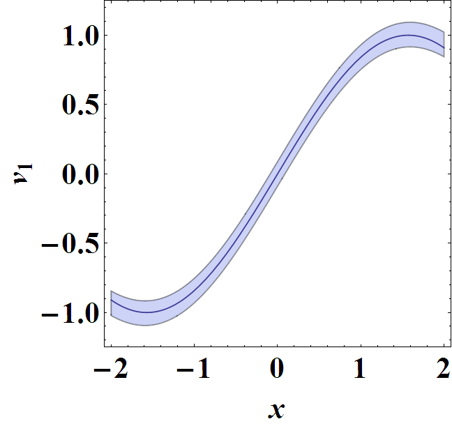
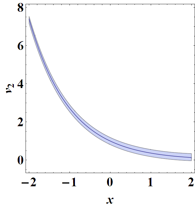
  Figure 1: Taylor polynomial approximation of elementary functions

  Then we can define $D_{\mathbf{y}}\,\,\widehat{=}\,\,D_{\mathbf{x}}\wedge\mathit{TM}_{\mathbf{x},\mathbf{v}}$. Thus we finally get a PDS $\mathcal{C}_{\mathbf{y}}\,\widehat{=}\,(\Xi_{\mathbf{y}},\mathbf{f}_{\mathbf{y}},$ $D_{\mathbf{y}})$ that simulates $\mathcal{C}_{\mathbf{x}}$. Note that here $\Xi_{\mathbf{y}}$ is not a subset of $D_{\mathbf{y}}$, which conflicts with our assumption on CDSs. However, allowing more behavior in $\mathcal{C}_{\mathbf{y}}$ does not affect the soundness of abstraction; besides, this problem can be easily remedied by taking $\Xi_{\mathbf{y}}\wedge D_{\mathbf{y}}$ as the initial set. We keep the current form for ease of safety verification in Section 4.

3.3 Abstracting EHSs by PHSs

In the previous sections, we have presented a method to abstract an EDS to a PDS such that the PDS simulates the EDS. Now we show, given an EHS $\mathcal{H}_{\mathbf{x}}$, how to construct a simulation map $\Theta$ and the corresponding PHS $\mathcal{H}_{\mathbf{y}}$ that simulates $\mathcal{H}_{\mathbf{x}}$. Actually, this can be easily done by just extending the previous abstraction approach a bit to take into account guard constraints and reset functions. Another difference is that we need to treat each mode of a HA separately by constructing an individual simulation map for each of them.

More specifically, given an EHS $\mathcal{H}_{\mathbf{x}}\,\widehat{=}\,(Q,X,f_{\mathbf{x}},D_{\mathbf{x}},$ $E,G_{\mathbf{x}},R_{\mathbf{x}},$ $\Xi_{\mathbf{x}})$, for each mode $q\in Q$, and for any $e\in E$ with $q$ the starting mode, we need to introduce new variables to replace all non-polynomial terms occurring in $\mathbf{f}_{\mathbf{x},q}$, $\Xi_{\mathbf{x},q}$, $D_{\mathbf{x},q}$, $G_{\mathbf{x},e}$ and $R_{\mathbf{x},e}$, and then compute the time derivatives of the fresh variables, as we did in the continuous case. In this way, for each mode $q$ we will obtain a vector of new variables $\mathbf{v}_{q}$ and the corresponding replacement equations $\mathbf{v}_{q}=\Gamma_{q}(\mathbf{x})$; without loss of generality, we can assume all $\mathbf{v}_{q}$ to be of the same dimension, and thus can get rid of the subscript $q$ of $\mathbf{v}_{q}$. At the same time, for all mode $q$, the elementary vector field $\mathbf{f}_{\mathbf{x},q}$ will be transformed into a polynomial one, i.e. $\tilde{\mathbf{f}}_{q}(\mathbf{x},\mathbf{v})$, as given by Proposition 1 and formula (12).

Let $\mathbf{y}\,\widehat{=}\,(\mathbf{x},\mathbf{v})$. Let $\Theta_{q}:D_{\mathbf{x},q}\rightarrow\mathbb{R}^{|\mathbf{y}|}$ be given by

$$\Theta_{q}(\mathbf{x})=(\mathbf{x},\Gamma_{q}(\mathbf{x}))\enspace.$$ (23)

Now the construction of $\mathcal{H}_{\mathbf{y}}\,\widehat{=}\,(Q,Y,f_{\mathbf{y}},D_{\mathbf{y}},E,G_{\mathbf{y}},R_{\mathbf{y}},\Xi_{\mathbf{y}})$ can proceed as follows.

• For each $q\in Q$, let

  $$\mathbf{f}_{\mathbf{y},q}(\mathbf{x},\mathbf{v})\,\,\widehat{=}\,\,\tilde{\mathbf{f}}_{q}(\mathbf{x},\mathbf{v})$$ (24)

  with $\tilde{\mathbf{f}}_{q}(\mathbf{x},\mathbf{v})$ given by (12).

• For each $q\in Q$, abstract $\mathbf{v}=\Gamma_{q}(\mathbf{x})$ in

  $$\Xi_{\mathbf{x},q}\llbracket\mathbf{v}/\Gamma_{q}(\mathbf{x})\rrbracket\wedge\mathbf{v}=\Gamma_{q}(\mathbf{x})$$ (25)

  and

  $$D_{\mathbf{x},q}\llbracket\mathbf{v}/\Gamma_{q}(\mathbf{x})\rrbracket\wedge\mathbf{v}=\Gamma_{q}(\mathbf{x})$$ (26)

  by polynomial expressions along the ways (W1)-(W4), and thus $\Xi_{\mathbf{y},q}$ and $D_{\mathbf{y},q}$ can be obtained.

• For each $e\in E$ with $q$ the starting mode, abstract $\mathbf{v}=\Gamma_{q}(\mathbf{x})$ in

  $$G_{\mathbf{x},e}\llbracket\mathbf{v}/\Gamma_{q}(\mathbf{x})\rrbracket\wedge\mathbf{v}=\Gamma_{q}(\mathbf{x})$$ (27)

  by polynomial expressions along the ways (W1)-(W4), and thus $G_{\mathbf{y},e}$ can be obtained.

So far, the only component left unspecified in $\mathcal{H}_{\mathbf{y}}$ is $R_{\mathbf{y},e}$.

• For each $e=(q,q^{\prime})\in E$, define

  $$\tilde{R}_{\mathbf{y},e}(\mathbf{x},\mathbf{v})\!\!\! \,\widehat{=} \!\!\!\{(\mathbf{x}^{\prime},\mathbf{v}^{\prime})\mid\mathbf{x}^{\prime}\in R_{\mathbf{x},e}(\mathbf{x})\llbracket\mathbf{v}/\Gamma_{q}(\mathbf{x})\rrbracket\wedge\,\enspace$$ (28)

  $$\!\quad\qquad\quad\mathbf{v}^{\prime}=\Gamma_{q^{\prime}}(\mathbf{x}^{\prime})\,\}\enspace.$$

  Then abstract $\mathbf{v}^{\prime}=\Gamma_{q^{\prime}}(\mathbf{x}^{\prime})$ in (28) by polynomial expressions along the ways (W1)-(W4), and thus $R_{\mathbf{y},e}$ can be obtained. For example, if (W4) is adopted then $R_{\mathbf{y},e}$ can be defined as

  $$R_{\mathbf{y},e}(\mathbf{x},\mathbf{v})\,\,\,\widehat{=}\,\,\,\{(\mathbf{x}^{\prime},\mathbf{v}^{\prime})\mid\mathbf{x}^{\prime}\in R_{\mathbf{x},e}(\mathbf{x})\llbracket\mathbf{v}/\Gamma_{q}(\mathbf{x})\rrbracket\}\enspace.$$

  In particular, if $R_{\mathbf{x},e}$ is an identity map and $\Gamma_{q}=\Gamma_{q^{\prime}}$, then $R_{\mathbf{y},e}$ is also an identity map.

Theorem 3.3 (Abstracting EHS by PHS)

Given an EHS $\mathcal{H}_{\mathbf{x}}\,\widehat{=}\,(Q,X,f_{\mathbf{x}},D_{\mathbf{x}},E,G_{\mathbf{x}},$ $R_{\mathbf{x}},\Xi_{\mathbf{x}})$, let $\mathcal{H}_{\mathbf{y}}\,\widehat{=}\,(Q,Y,$ $f_{\mathbf{y}},D_{\mathbf{y}},$ $E,$ $G_{\mathbf{y}},R_{\mathbf{y}},\Xi_{\mathbf{y}})$, where $\mathbf{f}_{\mathbf{y},q}$ is given by (24) and (12), and $\Xi_{\mathbf{y},q},D_{\mathbf{y},q},$ $G_{\mathbf{y},e},R_{\mathbf{y},e}$ are given by (25), (26), (27) and (28), together with (W1)-(W4), respectively. Then $\mathcal{H}_{\mathbf{y}}$ is a polynomial abstraction of $\mathcal{H}_{\mathbf{x}}$ in the sense of Definition 7, under the simulation maps $\Theta_{q}$ defined by (23).

Proof

First, it is easy to check that $\mathcal{H}_{\mathbf{y}}$ is a PHS. Second, by Theorem 3.2, we can get $(\Xi_{{\mathbf{y}},q},\mathbf{f}_{{\mathbf{y}},q},D_{{\mathbf{y}},q})$ simulates $(\Xi_{{\mathbf{x}},q},\mathbf{f}_{{\mathbf{x}},q},$ $D_{{\mathbf{x}},q})$ via $\Theta_{q}$, for each $q\in Q$. Third, from (27) and (W1)-(W4) it is easy to see that $\Theta_{q}(G_{{\mathbf{x}},e})\subseteq G_{{\mathbf{y}},e}$, for any $e=(q,q^{\prime})\in E$. By Definition 7, we finally need to show that $\Theta_{q^{\prime}}(R_{{\mathbf{x}},e}({\mathbf{x}}))\subseteq R_{{\mathbf{y}},e}(\Theta_{q}({\mathbf{x}}))$, for any $e=(q,q^{\prime})\in E$ and any ${\mathbf{x}}\in G_{\mathbf{x},e}$.

By (23) we have

$$\Theta_{q^{\prime}}(R_{{\mathbf{x}},e}({\mathbf{x}}))=\{(\mathbf{x}^{\prime},\mathbf{v}^{\prime})\mid\mathbf{x}^{\prime}\in R_{{\mathbf{x}},e}({\mathbf{x}})\wedge\mathbf{v}^{\prime}=\Gamma_{q^{\prime}}(\mathbf{x}^{\prime})\}\enspace.$$ (29)

By (28), (23) and (29) we have

$$\tilde{R}_{\mathbf{y},e}(\Theta_{q}(\mathbf{x}))=\tilde{R}_{\mathbf{y},e}(\mathbf{x},\Gamma_{q}(\mathbf{x}))=\Theta_{q^{\prime}}(R_{{\mathbf{x}},e}({\mathbf{x}}))\enspace.$$

By (W1)-(W4) we have $\tilde{R}_{\mathbf{y},e}(\Theta_{q}(\mathbf{x}))\subseteq R_{\mathbf{y},e}(\Theta_{q}(\mathbf{x}))$. Therefore we finally get
$\Theta_{q^{\prime}}(R_{{\mathbf{x}},e}({\mathbf{x}}))\subseteq R_{{\mathbf{y}},e}(\Theta_{q}({\mathbf{x}}))$. ∎

Example 2

Consider the example of a bouncing ball over a sine-waved surface as illustrated by the left picture in Figure 2, adapted from a similar one in [12]. The motion of the ball stays in the two-dimensional $x$-$y$ plane, with $x$ denoting the horizontal position and $y$ denoting the height, and the velocity along the two directions are denoted by $v_{x}$ and $v_{y}$ respectively. When the ball hits the surface given by the sine wave $y=\sin{x}$, its dynamics changes instantaneously. We assume the collision between the ball and the surface to be perfectly elastic so that there is no loss of energy. For instance, if the ball touches the surface at point $(0,0)$ with a downward vertical velocity $v_{y}$ and zero horizontal velocity $v_{x}$, then after collision $v_{y}$ becomes $0$ while $v_{x}$ takes the value of $v_{y}$ before collision.

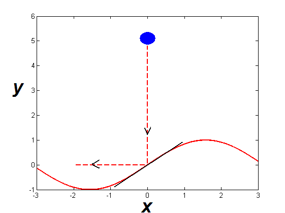
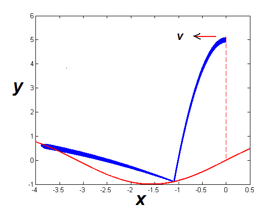
Figure 2: Bouncing ball on a sine-waved surface

As explained above, the HA model $\mathcal{H}_{\mathbf{x}}$ of the bouncing ball can be given as

• $Q=\{q\}$; $X=\{x,y,v_{x},v_{y}\}$;

• $E=\{e\}$ with $e=(q,q)$;

• $D_{\mathbf{x},q}\,\widehat{=}\,y\geqslant\sin{x}$; $G_{\mathbf{x},e}\,\widehat{=}\,y=\sin{x}$;

• $\Xi_{\mathbf{x},q}\,\widehat{=}\,y\geqslant 4.9\wedge y\leqslant 5.1\wedge x=0\wedge v_{x}=-1\wedge v_{y}=0$;

• $\mathbf{f}_{\mathbf{x},q}$ defines the ODE

  $$\left\{\begin{array}[]{lll}\dot{x}&=&v_{x}\\ \dot{y}&=&v_{y}\\ \dot{v}_{x}&=&0\\ \dot{v}_{y}&=&-9.8\end{array}\right.\enspace;$$ (30)

• $R_{\mathbf{x},e}(x,y,v_{x},v_{y})\,\widehat{=}\,\{(x,y,v_{x}^{\prime},v_{y}^{\prime})\}$ with

  $$\left\{\begin{array}[]{lll}v_{x}^{\prime}&=&\frac{(\sin{x})^{2}\cdot v_{x}+2(\cos{x})\cdot v_{y}}{1+(\cos{x})^{2}}\\ v_{y}^{\prime}&=&\frac{2(\cos{x})\cdot v_{x}-(\sin{x})^{2}\cdot v_{y}}{1+(\cos{x})^{2}}\\ \end{array}\right.\enspace.$$ (31)

Note that in the above model, non-polynomial expressions exist in $D_{q},G_{e}$ and $R_{e}$. By applying our proposed abstraction approach, we obtained the replacement equations $(u_{1},u_{2},u_{3})=(\sin{x},$ $\cos{x},\frac{1}{1+(\cos{x})^{2}})$, and the PHS $\mathcal{H}_{\mathbf{y}}$:

• $Q$ and $E$ are the same as $\mathcal{H}_{\mathbf{x}}$;

• $Y=\{x,y,v_{x},v_{y},u_{1},u_{2},u_{3}\}$;

• $D_{\mathbf{y},q}\,\widehat{=}\,y\geqslant u_{1}$; $G_{\mathbf{y},e}\,\widehat{=}\,y=u_{1}$; note that here we adopt (W4) when abstracting $D_{\mathbf{x},q}$ and $G_{\mathbf{x},e}$;

• $\Xi_{\mathbf{y},q}\,\widehat{=}\,\Xi_{\mathbf{x},q}\wedge u_{1}=0\wedge u_{2}=1\wedge u_{3}=0.5$;

• $\mathbf{f}_{\mathbf{y},q}$ defines the ODE

  $$\left\{\begin{array}[]{lll}\dot{x}&=&v_{x}\\ \dot{y}&=&v_{y}\\ \dot{v}_{x}&=&0\\ \dot{v}_{y}&=&-9.8\\ \dot{u}_{1}&=&u_{2}v_{x}\\ \dot{u}_{2}&=&-u_{1}v_{x}\\ \dot{u}_{3}&=&2u_{1}u_{2}u_{3}^{2}v_{x}\end{array}\right.\enspace;$$ (32)

• $R_{\mathbf{y},e}(\mathbf{y})\,\widehat{=}\,\{(x,y,v_{x}^{\prime},v_{y}^{\prime},u_{1},u_{2},u_{3})\}$ with

  $$\left\{\begin{array}[]{lll}v_{x}^{\prime}&=&u_{3}\cdot(u_{1}^{2}\cdot v_{x}+2u_{2}\cdot v_{y})\\ v_{y}^{\prime}&=&u_{3}\cdot(2u_{2}\cdot v_{x}-u_{1}^{2}\cdot v_{y})\\ \end{array}\right.\enspace;$$ (33)

  note that $u_{1},u_{2},u_{3}$ are only related to $x$ which is reset to itself, and thus the resets of $u_{1},u_{2},u_{3}$ are identity mappings.

Once we get the polynomial abstraction $\mathcal{H}_{\mathbf{y}}$, we can use existing tools for PHSs to analyze its behavior. Here we use the state-of-the-art nonlinear hybrid system analyzer Flow^∗ [5]. The right picture in Figure 2 shows the computed reachable set over-approximation (projected to the $x$-$y$ plane) of $\mathcal{H}_{\mathbf{y}}$ within two jumps, which is also the reachable set over-approximation of $\mathcal{H}_{\mathbf{x}}$ by Theorem 2.1. Note that such an analysis would NOT have been possible directly on $\mathcal{H}_{\mathbf{x}}$ in Flow^∗ since its current version does not support elementary functions in domains, guards, or reset functions.

4 Application in Safety Verification of EHSs

One of the mostly studied problems in the study of HSs is safety verification. Given a HS $\mathcal{H}$, a safety requirement for $\mathcal{H}$ can be specified as $\mathcal{S}\,\widehat{=}\,\bigcup_{q\in Q}(\{q\}\times S_{q})$ with $S_{q}\subseteq\mathbb{R}^{n}$ the safe region of mode $q$. Alternatively, a safety property can be given as a set of unsafe regions $\mathcal{US}\,\widehat{=}\,\bigcup_{q\in Q}(\{q\}\times\bar{S_{q}})$ with $\bar{S_{q}}$ the complement of $S_{q}$ in $\mathbb{R}^{n}$. The safety verification problem asks whether $\mathcal{R}_{\mathcal{H}}\subseteq\mathcal{S}$, or equivalently, whether $\mathcal{R}_{\mathcal{H}}\cap\mathcal{US}=\emptyset$.

The following result relates the safety verification problem of a HS $\mathcal{H}_{\mathbf{x}}$ to that of $\mathcal{H}_{\mathbf{y}}$ which simulates $\mathcal{H}_{\mathbf{x}}$.

Theorem 4.1 (Safety Relation)

Let $\mathcal{US}_{\mathbf{x}}\,\widehat{=}\,\bigcup_{q}(\{q\}\times\bar{S}_{\mathbf{x},q})$ be a safety requirement of the HS $\mathcal{H}_{\mathbf{x}}$. Suppose $\mathcal{H}_{\mathbf{y}}$ simulates $\mathcal{H}_{\mathbf{x}}$ via simulation maps $\{\Theta_{q}\mid q\in Q\}$. Let $\mathcal{US}_{\mathbf{y}}\,\widehat{=}\,\bigcup_{q}(\{q\}\times\bar{S}_{\mathbf{y},q})$ with $\bar{S}_{\mathbf{y},q}\supseteq\Theta_{q}(\bar{S}_{\mathbf{x},q})$. Then if $\mathcal{H}_{\mathbf{y}}$ is safe w.r.t. $\mathcal{US}_{\mathbf{y}}$, then $\mathcal{H}_{\mathbf{x}}$ is safe w.r.t. $\mathcal{US}_{\mathbf{x}}$.

Proof

Let $\mathcal{R}_{\mathbf{x}}$ and $\mathcal{R}_{\mathbf{y}}\,\widehat{=}\,\bigcup_{q}(\{q\}\times H_{\mathbf{y},q})$ denote the reachable sets of $\mathcal{H}_{\mathbf{x}}$ and $\mathcal{H}_{\mathbf{y}}$ respectively. Suppose $\mathcal{R}_{\mathbf{y}}\cap\mathcal{US}_{\mathbf{y}}=\emptyset$, i.e. $H_{\mathbf{y},q}\cap\bar{S}_{\mathbf{y},q}=\emptyset$ for any $q\in Q$. Thus $\Theta_{q}^{-1}(H_{\mathbf{y},q})$ $\cap\,\Theta_{q}^{-1}(\bar{S}_{\mathbf{y},q})=\emptyset$, which implies

$$\Theta_{q}^{-1}(H_{\mathbf{y},q})\cap\,\Theta_{q}^{-1}\big{(}\Theta_{q}(\bar{S}_{\mathbf{x},q})\big{)}=\emptyset\enspace.$$

Therefore $\Theta_{q}^{-1}(H_{\mathbf{y},q})\cap\bar{S}_{\mathbf{x},q}=\emptyset$. By Theorem 2.1 we get $\mathcal{R}_{\mathbf{x}}\subseteq\bigcup_{q\in Q}\big{(}\{q\}\times\Theta_{q}^{-1}(H_{\mathbf{y},q})\big{)}$. Thus $\mathcal{R}_{\mathbf{x}}\cap\mathcal{US}_{\mathbf{x}}=\emptyset$.∎

Note that if the safety properties of EHSs are not in polynomial forms but contain elementary functions, we can replace the non-polynomial terms by new variables when constructing the simulation map, as we do for the EHSs themselves.

Theorem 4.1 allows us to take advantage of constraint-based approaches for PHSs to verify safety properties of EHSs. In the rest of this section, we show how to perform safety verification for EHSs by combining the previous proposed polynomial abstraction method with constraint-based verification techniques for PHSs.

4.1 Generating Polynomial Invariants

In this and next subsections, for simplicity, we will use EDSs as special cases of EHSs to illustrate how to generate inductive invariants for safety verification of EHSs.

Given an EDS $\mathcal{C}_{\mathbf{x}}\,\widehat{=}\,(\Xi_{\mathbf{x}},\mathbf{f}_{\mathbf{x}},D_{\mathbf{x}})$ and an unsafe region $\bar{S}_{\mathbf{x}}$, we first construct a PDS $\mathcal{C}_{\mathbf{y}}\,\widehat{=}\,(\Xi_{\mathbf{y}},\mathbf{f}_{\mathbf{y}},D_{\mathbf{y}})$ that simulates $\mathcal{C}_{\mathbf{x}}$, as well as the polynomial abstraction $\bar{S}_{\mathbf{y}}$ of $\bar{S}_{\mathbf{x}}$. According to Theorem 2.1 and 4.1, if we can find a semi-algebraic inductive invariant $P(\mathbf{y})=P(\mathbf{x},\mathbf{v})$ for $\mathcal{C}_{\mathbf{y}}$ with $\mathbf{v}=\Gamma(\mathbf{x})$ the replacement equations, such that $P(\mathbf{x},\mathbf{v})$ is a certificate of the safety of $\mathcal{C}_{\mathbf{y}}$ w.r.t. $\bar{S}_{\mathbf{y}}$, then $P(\mathbf{x},\Gamma(\mathbf{x}))$ is an inductive invariant certificate of the safety of $\mathcal{C}_{\mathbf{x}}$ w.r.t. $\bar{S}_{\mathbf{x}}$. If $P(\mathbf{x},\mathbf{v})$ does contain variables $\mathbf{v}$, then $P(\mathbf{x},\Gamma(\mathbf{x}))$ gives an elementary invariant of $\mathcal{C}_{\mathbf{x}}$; otherwise $P(\mathbf{x},\Gamma(\mathbf{x}))$ is just a polynomial invariant.

The form of the invariant $P(\mathbf{y})$ of $\mathcal{C}_{\mathbf{y}}$ determines not only what kinds of invariants we can get for $\mathcal{C}_{\mathbf{x}}$, but also the selection of abstraction ways (W1)-(W4) in Section 3.2. To see this, we first assume for $\mathcal{C}_{\mathbf{y}}$ a polynomial invariant candidate $P(\mathbf{u},\mathbf{x})\,\widehat{=}\,p(\mathbf{u},\mathbf{x})\leqslant 0$ without the fresh variables $\mathbf{v}$, where $\mathbf{u}$ is the vector of parameters to be determined. Then a typical set of constraints on $\mathbf{u}$ given by the constraint-based verification approach could be as follows:

• $\forall\mathbf{x}\forall\mathbf{v}.(\Xi_{\mathbf{y}}\longrightarrow P(\mathbf{u},\mathbf{x}))$;

• $\forall\mathbf{x}\forall\mathbf{v}.(D_{\mathbf{y}}\longrightarrow\nabla p(\mathbf{u},\mathbf{x})\cdot\mathbf{f}_{\mathbf{y}}\leqslant 0)$;

• $\forall\mathbf{x}\forall\mathbf{v}.(P(\mathbf{u},\mathbf{x})\longrightarrow\neg\bar{S}_{\mathbf{y}})$.

By (W1)-(W4), it is easy to check that $(\exists\mathbf{v}.\Xi_{\mathbf{y}})\Longleftrightarrow\Xi_{\mathbf{x}}$. Then we can prove that (C1) is equivalent to $\forall\mathbf{x}.(\Xi_{\mathbf{x}}\longrightarrow P(\mathbf{u},\mathbf{x}))$. Similarly, by $(\exists\mathbf{v}.\bar{S}_{\mathbf{y}})\Longleftrightarrow\bar{S}_{\mathbf{x}}$, we can prove that (C3) is equivalent to $\forall\mathbf{x}.(P(\mathbf{u},\mathbf{x})\longrightarrow\neg\bar{S}_{\mathbf{x}})$. Therefore we can conclude that it is sufficient to adopt (W4) for the abstraction of $\Xi_{\mathbf{x}}$ and $\bar{S}_{\mathbf{x}}$. The gradient $\nabla p(\mathbf{u},\mathbf{x})$ in (C2) is computed w.r.t. variables $\mathbf{y}=(\mathbf{x},\mathbf{v})$. Since $p(\mathbf{u},\mathbf{x})$ does not contain $\mathbf{v}$, all the partial derivatives of $p(\mathbf{u},\mathbf{x})$ w.r.t. $\mathbf{v}$ are zero. The consequence of this fact is twofold: first, only those components of $\mathbf{f}_{\mathbf{y}}$ that define the derivatives of $\mathbf{x}$, i.e. $\mathbf{f}_{\mathbf{x}}\llbracket\mathbf{v}/\Gamma(\mathbf{x})\rrbracket$, are relative to the computation of $p(\mathbf{u},\mathbf{x})\cdot\mathbf{f}_{\mathbf{y}}$, which means we do not even need to compute the derivatives of the fresh variables $\mathbf{v}$ when constructing $\mathbf{f}_{\mathbf{y}}$; second, only those fresh variables occurring in $\mathbf{f}_{\mathbf{x}}\llbracket\mathbf{v}/\Gamma(\mathbf{x})\rrbracket$ will occur in $p(\mathbf{u},\mathbf{x})\cdot\mathbf{f}_{\mathbf{y}}$, and then from (C2) we can prove that when constructing $D_{\mathbf{y}}$, the variables do not exist in $p(\mathbf{u},\mathbf{x})\cdot\mathbf{f}_{\mathbf{y}}$ can be simply abstracted away.

In summary, assuming an invariant template $P(\mathbf{u},\mathbf{x})$ without fresh variables $\mathbf{v}$ can greatly simplify the construction of $\mathcal{C}_{\mathbf{y}}$, and enables us to generate polynomial invariants for $\mathcal{C}_{\mathbf{x}}$.

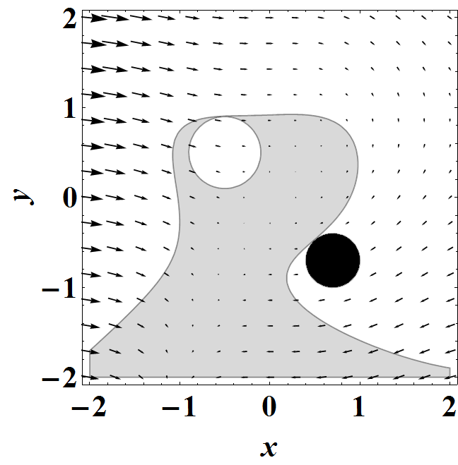
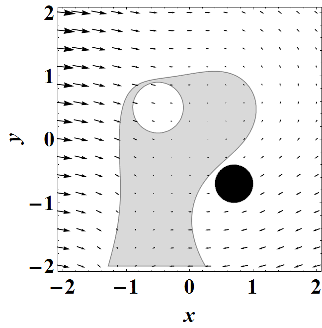
Figure 3: Comparison of polynomial and elementary inductive invariants

Example 3

Consider the EDS $\mathcal{C}_{\mathbf{x}}$ in Example 1. We will try to generate a polynomial inductive invariant to verify the safety of $\mathcal{C}_{\mathbf{x}}$ w.r.t. an unsafe region $\bar{S}_{\mathbf{x}}\,\widehat{=}\,(x-0.7)^{2}+(y+0.7)^{2}-0.09\leqslant 0$. By the above discussion, the PDS abstraction $\mathcal{C}_{\mathbf{y}}$ of $\mathcal{C}_{\mathbf{x}}$ can be defined by

$$\mathcal{C}_{\mathbf{y}}\quad\widehat{=}\quad\big{(}\Xi_{\mathbf{x}},\mathbf{f}_{\mathbf{x}}\llbracket\mathbf{v}/\Gamma(\mathbf{x})\rrbracket,D_{\mathbf{x}}\wedge(\ref{eqn:taylor-sin-x})\wedge(\ref{eqn:taylor-exp-x})\big{)}$$

with $\mathbf{v}=\Gamma(\mathbf{x})$ given by (19). The unsafe region for $\mathcal{C}_{\mathbf{y}}$ is $\bar{S}_{\mathbf{y}}\,\widehat{=}\,\bar{S}_{\mathbf{x}}$.

By applying the SOS-relaxation-based invariant generation approach [25, 16] with a polynomial template $p(\mathbf{u},x,y)\leqslant 0$ of degree 5 (in $x,y$) and using the Matlab-based tool YALMIP [19] and SeDuMi [33] (or SDPT3 [35]), we successfully generated an invariant that verifies $\neg\bar{S}_{\mathbf{x}}$ for $\mathcal{C}_{\mathbf{x}}$. Please see the left part of Figure 3 for an illustration of $\mathbf{f}_{\mathbf{x}}$ (the black arrows), $D_{\mathbf{x}}$ (the outer white box), the synthesized invariant $p(x,y)\leqslant 0$ (the grey area with curved boundary), $\Xi_{\mathbf{x}}$ (the white circle inside the invariant) and $\bar{S}_{\mathbf{x}}$ (the black circle outside the invariant). The explicit form of $p(x,y)$ is:

$$p(x,y) := \scriptstyle-29.5258683+2.7905x-15.4285y+7.7870x^{2}-20.4040xy$$

$$\scriptstyle+22.4031y^{2}+14.0762x^{3}-18.7539x^{2}y+41.8913xy^{2}+5.9623y^{3}$$

$$\scriptstyle+25.8881x^{4}+4.5276x^{3}y+2.6340x^{2}y^{2}-21.2871xy^{3}+5.6462y^{4}$$

$$\scriptstyle-9.8303x^{5}+0.8716x^{4}y+1.4942x^{3}y^{2}+9.9083x^{2}y^{3}-11.0499xy^{4}$$

$$\scriptstyle+24.5758y^{5}\qquad.$$

4.2 Generating Elementary Invariants

Now we show how to generate elementary invariants for $\mathcal{C}_{\mathbf{x}}$ in Example 3.

Example 4

Consider the EDS $\mathcal{C}_{\mathbf{x}}$ and unsafe region $\bar{S}_{\mathbf{x}}$ in Example 3. This time we try to generate an inductive invariant for $\mathcal{C}_{\mathbf{y}}$ using the template $p(\mathbf{u},\mathbf{x},\mathbf{v})\leqslant 0$ with all the variables $\mathbf{v}$ included. According to constraints similar to (C1)-(C3), it requires a more refined abstraction of $\mathcal{C}_{\mathbf{x}}$ to reflect the relations between $\mathbf{x}$ and $\mathbf{v}$. Here we adopt (W2) for the abstraction of $\Xi_{\mathbf{x}},D_{\mathbf{x}}$ and $\bar{S}_{\mathbf{x}}$. We define $D_{\mathbf{y}}$ to be the same one as in Example 1. From $\Xi_{\mathbf{x}}$ it can be deduced that $(x,y)\in B_{\Xi}\,\widehat{=}\,[-0.9,-0.1]\times[0.1,0.9]$ for any $(x,y)\in\Xi_{\mathbf{x}}$. Then we can compute the Taylor polynomials of $\mathbf{v}=\Gamma(\mathbf{x})$ over $B_{\Xi}$, and thus get $\Xi_{\mathbf{y}}$. The abstraction $\bar{S}_{\mathbf{y}}$ of $\bar{S}_{\mathbf{x}}$ can be obtained similarly. The vector field $\mathbf{f}_{\mathbf{y}}$ is given by (20).

Using a template $p(\mathbf{u},\mathbf{x},\mathbf{v})\leqslant 0$ with $p(\mathbf{u},\mathbf{x},\mathbf{v})$ a parametric polynomial of degree 3 (in $\mathbf{x},\mathbf{v}$), we finally obtained an invariant $p(x,y,v_{1},v_{2},v_{3})\leqslant 0$ that verifies $\neg\bar{S}_{\mathbf{y}}$ for $\mathcal{C}_{\mathbf{y}}$, which means $p(x,y,\sin{x},e^{-x},\cos{x})\leqslant 0$ is an invariant of $\mathcal{C}_{\mathbf{x}}$ that verifies $\neg\bar{S}_{\mathbf{x}}$. The right part of Figure 3 is an illustration of $p(x,y,\sin{x},e^{-x},\cos{x})\leqslant 0$. The explicit form of $p(x,y,v_{1},v_{2},v_{3})$ is:

$$p := \scriptstyle-4.955995973+2.6956x-7.7162y+1.3633v_{1}-1.1243v_{2}-1.0806v_{3}+0.6966x^{2}-8.9155xy+5.8828y^{2}$$

$$\scriptstyle+3.0691xv_{1}-3.6545yv_{1}+0.2592v_{1}^{2}-3.3022xv_{2}+1.4964yv_{2}-0.7498v_{1}v_{2}-4.2837v_{2}^{2}-0.2079xv_{3}$$

$$\scriptstyle-7.7557yv_{3}-1.5121v_{1}v_{3}+1.5754v_{2}v_{3}-1.3813v_{3}^{2}-0.0353x^{3}-0.3128x^{2}y+0.9184xy^{2}+6.6938y^{3}$$

$$\scriptstyle-0.1410x^{2}v_{1}+3.1509xyv_{1}+1.8136y^{2}v_{1}+6.5973xv_{1}^{2}+7.7242yv_{1}^{2}+1.7114v_{1}^{3}-1.0877x^{2}v_{2}+4.4452xyv_{2}$$

$$\scriptstyle+1.2358y^{2}v_{2}+1.3919xv_{1}v_{2}+7.9981yv_{1}v_{2}+2.5635v_{1}^{2}v_{2}-0.8835xv_{2}^{2}+1.4900yv_{2}^{2}+0.0392v_{1}v_{2}^{2}+1.1281v_{2}^{3}$$

$$\scriptstyle-1.8619x^{2}v_{3}-2.4300xyv_{3}+2.2032y^{2}v_{3}-2.5384xv_{1}v_{3}-6.2048yv_{1}v_{3}-4.9447v_{1}^{2}v_{3}+1.6193xv_{2}v_{3}$$

$$\scriptstyle+1.2933yv_{2}v_{3}-0.5207v_{1}v_{2}v_{3}-0.2498v_{2}^{2}v_{3}+5.8866xv_{3}^{2}+5.1296yv_{3}^{2}+0.7890v_{1}v_{3}^{2}+2.0905v_{2}v_{3}^{2}-2.3259v_{3}^{3}\enspace.$$

We can see that the elementary invariant is sharper than the polynomial invariant and separates better from the unsafe region. This indicates that by allowing non-polynomial terms in templates, invariants of higher quality may be generated and thus increases the possibility of verifying safety properties of EHSs. Moreover, it also suggests that even for purely polynomial systems, one could assume any kind of elementary terms in a predefined template when generating invariants, which gives a more general method than [28, 9] for generating elementary invariants for PHSs.

4.3 More Experiments

We have implemented the proposed abstraction approach (not including the part on abstraction of replacement equations) and experimented with it using the following examples on safety verification for EHSs. The formal abstraction algorithms can be found in the appendix, and all the input files for the experiments can be obtained at http://lcs.ios.ac.cn/%7Ezoul/casestudies/fm2015.zip

Example 5 (HIV Transmission)

The following continuous dynamics, with the assumption that there is no recruitment of population, has been developed to model HIV transmission [2]

$$\mathbf{f}\,\widehat{=}\,\left\{\begin{array}[]{lll}\dot{u}_{1}&=&-\frac{\beta cu_{1}u_{2}}{u_{1}+u_{2}+u_{3}}-\mu u_{1}\\ \dot{u}_{2}&=&\frac{\beta cu_{1}u_{2}}{u_{1}+u_{2}+u_{3}}-(\mu+\nu)u_{2}\\ \dot{u}_{3}&=&\nu u_{2}-\alpha u_{3}\end{array}\right.\enspace,$$ (34)

where $u_{1}(t),u_{2}(t),u_{3}(t)$ denote the part of population that is HIV susceptible, HIV infected, and that has AIDS respectively, $\beta$ is the possibility of infection per partner contact, $c$ is the rate of partner change, $\mu$ is the death rate of non-AIDS population, $\alpha$ is the death rate of AIDS patients, and $\nu$ is the rate at which HIV infected people develop AIDS. Note that the dynamics involves non-polynomial term $\frac{1}{u_{1}+u_{2}+u_{3}}$. In this paper, the parameters are chosen to be $\beta=0.2,c=10,\mu=0.008,\alpha=0.95,\nu=0.1$. We want to verify that with the initial set

$$\Xi\,\widehat{=}\,u_{1}\in[9.985,9.995]\wedge u_{2}\in[0.005,0.015]\wedge u_{3}\in[0,0.003],$$

the population of AIDS patients alive will always be below 1 (the population is measured in thousands). That is, the system $(\Xi,\mathbf{f},D)$ satisfies $S\,\widehat{=}\,u_{3}\leqslant 1$, where $D\,\widehat{=}\,u_{1}\geqslant 0\wedge u_{2}\geqslant 0\wedge u_{3}\geqslant 0\wedge 0<u_{1}+u_{2}+u_{3}\leqslant 10.013\,.$

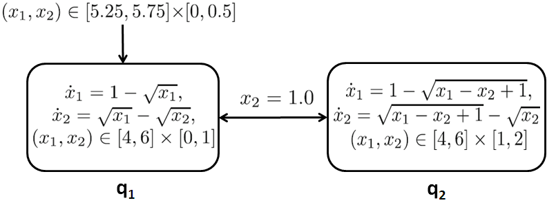
Figure 4: HA model of the two-tanks system

Example 6 (Two-Tanks)

The two-tanks system shown in Figure 4 comes from [34] and has been studied in [27, 12, 6] as a benchmark for safety verification of hybrid systems. It models two connected tanks, the liquid levels of which are denoted by $x_{1}$ and $x_{2}$ respectively. The system switches from mode $q_{1}$ (or $q_{2}$) to $q_{2}$ (or $q_{1}$) when $x_{2}$ reaches 1 at $q_{1}$ (or $q_{2}$). The system’s dynamics involve non-polynomial terms such as $\sqrt{x_{1}}$ or $\sqrt{x_{1}-x_{2}+1}$. The verification objective is to show that starting from mode $q_{1}$ with the initial set $\Xi_{q_{1}}\,\widehat{=}\,5.25\leqslant x_{1}\leqslant 5.75\wedge 0\leqslant x_{2}\leqslant 0.5$, the system will never reach the unsafe set $\bar{S}_{q_{1}}\,\widehat{=}\,(x_{1}-4.25)^{2}+(x_{2}-0.25)^{2}-0.0625\leqslant 0$ when staying at mode $q_{1}$.

Example 7 (Lunar Lander)

Consider a real-world example of the guidance and control of a lunar lander [36], as illustrated by Figure 5. The dynamics of the lander is given by

$$\mathbf{f}\,\widehat{=}\,\left\{\begin{array}[]{lll}\dot{v}&=&\frac{F_{c}}{m}-1.622\\ \dot{m}&=&-\frac{F_{c}}{2500}\\ \dot{F}_{c}&=&0\\ \dot{t}&=&1\end{array}\right.\enspace,$$ (35)

where $v$ and $m$ denote the vertical velocity and mass of the lunar lander; $F_{c}$ denotes the thrust imposed on the lander, which is kept constant during one sampling cycle of length 0.128 seconds; at each sampling point, $F_{c}$ is updated according to the guidance law shown in the right part of Figure 5.

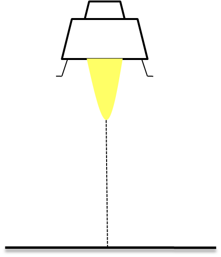
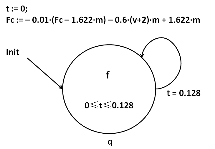
Figure 5: The lunar lander and its guidance-control system

Note that the derivative of $v$ involves non-polynomial expression $\frac{1}{m}$. We want to verify that with the initial condition $t=0$s, $v=-2$m/s, $m=1250$kg, $F_{c}=2027.5$N, the vertical velocity of the lunar lander will be kept around the target velocity $-$2m/s, i.e. $|v-(-2)|\leqslant\varepsilon$, where $\varepsilon=0.05$ is the specified bound for fluctuation of $v$.

Using the proposed abstraction method and the SOS-relaxation-based invariant generation method, we have successfully verified all the above 3 examples. The time costs on the platform with Intel Core i5-3470 CPU and 4GB RAM running Windows 7 are shown in Table 1.

Table 1: Time costs of invariant generation and safety verification for EHSs

example	E.g. 3	E.g. 4	E.g. 5	E.g. 6	E.g. 7
time cost (s)	1.324	7.994	5.186	0.977	2.645

Besides, we have also compared with the performances of the EHS verification tools HSOLVER [27], Flow^∗ [5], dReach [7] and iSAT-ODE [6] on these examples. The results are obtained on the same platform as above except for running Ubuntu Linux 14.04. In Table 2, time is measured in seconds; $-$ means that the verification fails, either because of abnormal termination due to error inflation, or because of non-termination within reasonable amount of time (several hours).

Table 2: Verification results of different methods

	EHS2PHS	HSOLVER	Flow∗	dReach	iSAT-ODE
E.g. 3	1.324	0.723	$-$	$-$	$-$
E.g. 5	5.186	$-$	$-$	$-$	$-$
E.g. 6	0.977	0.452	76.880	21.949	0.988
E.g. 7	2.645	$-$	20.238	$-$	63.648

From Table 2 we can see that the time costs of the proposed abstraction approach are all acceptable, whereas there do exist examples that existing approaches cannot solve effectively.

5 Conclusions

In this paper, we presented an approach to reducing an EHS to a PHS by variable transformation, and established the simulation relation between them, so that safety verification of the EHS can be reduced to that of the corresponding PHS. Thus our work enables all the well-established techniques for PHS verification to be applicable to EHSs. In particular, combined with invariant-based approach to safety verification for PHSs, it provides the possibility of overcoming the limitations of existing EHS verification approaches. Experimental results on real-world examples indicated the effectiveness of our approach.

A possible drawback of the proposed approach is that the SOS-based method may cause an incorrect invariant to be generated due to numerical computation errors. To overcome this, we have verified all the synthesized invariants posteriorly using symbolic computation tools.

Abstraction Algorithms

0:  An elementary expression expr and a set of equations eqs as input

0:  The returned expression is polynomial, and equals to the input expression in the context of equations eqs

1:  if $\textit{expr}=c$ or $\textit{expr}=x$ then

2:     return  $(\textit{expr},\textit{eqs})$;

3:  else if $\textit{expr}=\frac{\textit{expr}_{1}}{\textit{expr}_{2}}$ then

4:     $(\textit{expr}_{2},\textit{eqs})=\textbf{VT}(\textit{expr}_{2},eqs)$; return $\textbf{VT}(\textit{expr}_{1}*\textit{new\!Var}$, $\textit{eqs}.\textbf{add}(\textit{new\!Var},\frac{1}{\textit{expr}_{2}})$);

5:  else if $\textit{expr}=\textit{expr}_{1}^{\frac{\textit{n}_{1}}{\textit{n}_{2}}}$ then

6:     $(\textit{expr}_{1},\textit{eqs})=\textbf{VT}(\textit{expr}_{1},eqs)$; return ($\textit{new\!Var}^{\textit{n}_{1}}$, $\textit{eqs}.\textbf{add}(\textit{new\!Var},\textit{expr}_{1}^{\frac{1}{\textit{n}_{2}}})$);

7:  else if $\textit{expr}=e^{\textit{expr}_{1}}$ then

8:     $(\textit{expr}_{1},\textit{eqs})=\textbf{VT}(\textit{expr}_{1},eqs)$; return (new​Var, $\textit{eqs}.\textbf{add}(\textit{new\!Var},e^{\textit{expr}_{1}})$);

9:  else if $\textit{expr}=\ln(\textit{expr}_{1})$ then

10:     $(\textit{expr}_{1},\textit{eqs})=\textbf{VT}(\textit{expr}_{1},eqs)$; return (new​Var, $\textit{eqs}.\textbf{add}(\textit{new\!Var},\ln(\textit{expr}_{1}))$);

11:  else if $\textit{expr}=\sin(\textit{expr}_{1})$ then

12:     $(\textit{expr}_{1},\textit{eqs})=\textbf{VT}(\textit{expr}_{1},eqs)$; return (new​Var, $\textit{eqs}.\textbf{add}(\textit{new\!Var},\sin(\textit{expr}_{1}))$);

13:  else if $\textit{expr}=\cos(\textit{expr}_{1})$ then

14:     $(\textit{expr}_{1},\textit{eqs})=\textbf{VT}(\textit{expr}_{1},eqs)$; return (new​Var, $\textit{eqs}.\textbf{add}(\textit{new\!Var},\cos(\textit{expr}_{1}))$);

15:  else if $\textit{expr}=\textit{expr}_{1}+\textit{expr}_{1}$ then

16:     $(\textit{expr}_{1},\textit{eqs})=\textbf{VT}(\textit{expr}_{1},eqs)$; $(\textit{expr}_{2},\textit{eqs})=\textbf{VT}(\textit{expr}_{2},eqs)$;

17:     return  ($\textit{expr}_{1}+\textit{expr}_{2}$,eqs);  

18:  else if $\textit{expr}=\textit{expr}_{1}-\textit{expr}_{1}$ then

19:     $(\textit{expr}_{1},\textit{eqs})=\textbf{VT}(\textit{expr}_{1},eqs)$; $(\textit{expr}_{2},\textit{eqs})=\textbf{VT}(\textit{expr}_{2},eqs)$;

20:     return  ($\textit{expr}_{1}-\textit{expr}_{2}$,eqs);  

21:  else

22:     $(\textit{expr}_{1},\textit{eqs})=\textbf{VT}(\textit{expr}_{1},eqs)$; $(\textit{expr}_{2},\textit{eqs})=\textbf{VT}(\textit{expr}_{2},eqs)$;

23:     return  ($\textit{expr}_{1}\times\textit{expr}_{2}$, eqs);

24:  end if

Algorithm 1 Reducing an elementary expression to a polynomial one (VT(expr, eqs))

In Algorithm 1, new​Var denotes a fresh variable, and eqs records the replacements during the variable transformation.

0:  Polynomial differential equations $odes$ and a set of equations eqs as input (where all expressions in eqs are polynomial except the outermost operator)

0:  The resulting polynomial differential equations simulate the initial $odes$ and eqs

1:  for $(\textit{var},\textit{expr})$ in eqs do

2:     if $\textit{expr}=\frac{1}{\textit{expr}_{2}}$ then

3:        $odes.\textbf{add}(\textit{var},-\textit{var}^{2}*\dot{\textit{expr}_{2}})$;

4:     else if $\textit{expr}=\textit{expr}_{1}^{\frac{1}{\textit{n}_{2}}}$ then

5:        $\textit{eqs}.\textbf{add}(\textit{new\!Var},1/\textit{expr})$;  $odes.\textbf{add}(\textit{var},\frac{1}{\textit{n}_{2}}*\textit{new\!Var}^{\textit{n}_{2}-1}*\dot{\textit{expr}_{1}})$;

6:     else if $\textit{expr}=e^{\textit{expr}_{1}}$ then

7:        $odes.\textbf{add}(\textit{var},\textit{var}*\dot{\textit{expr}_{1}})$;

8:     else if $\textit{expr}=\ln(\textit{expr}_{1})$ then

9:        $\textit{eqs}.\textbf{add}(\textit{new\!Var},\frac{1}{\textit{expr}_{1}})$;  $odes.\textbf{add}(\textit{var},\textit{new\!Var}*\dot{\textit{expr}_{1}})$;

10:     else if $\textit{expr}=\sin(\textit{expr}_{1})$ then

11:        $\textit{eqs}.\textbf{add}(\textit{new\!Var},\cos(\textit{expr}_{1}))$;  $odes.\textbf{add}(\textit{var},\textit{new\!Var}*\dot{\textit{expr}_{1}})$;

12:     else if $\textit{expr}=\cos(\textit{expr}_{1})$ then

13:        $\textit{eqs}.\textbf{add}(\textit{new\!Var},\sin(\textit{expr}_{1}))$;  $odes.\textbf{add}(\textit{var},-\textit{new\!Var}*\dot{\textit{expr}_{1}})$;

14:     else

15:        The algorithm should not run this branch;

16:     end if

17:  end for

18:  return  $odes$;

Algorithm 2 Updating the dynamical system according to the replacement equations eqs (U(odes, eqs))

In Algorithm 2, op, left, and right returns the outermost operation, and its left and right operands for a given expression, respectively. left and right return the operand in case the outmost operation is one ary; new​Var denotes a fresh variable. Algorithm 2 must terminate, because the number of elements of eqs can only increase finite times, obviously, no more than the number of the subexpressions of the EDS.

0:  ODEs odes and a list of replacement equations eqs as input

0:  The resulting ODEs are polynomial

1:  for $ode$ in $odes$ do

2:     for $exp$ in $\textbf{omExp}(ode)$ do

3:        (exp, eqs) = VT(exp, eqs);

4:     end for

5:  end for

6:  return U(odes, eqs);

Algorithm 3 Transforming elementary ODEs to polynomial ODEs (TransEODEs(odes, eqs))

In algorithm 3, $\textbf{omExp}(ode)$ returns the set of the outmost expressions of $ode$, and VT and U call Algorithm 1 and 2, respectively.

0:  An elementary hybrid system hs as input

0:  The resulting hybrid system is a PHS which simulates the input EHS

1:  Set $eqs$ to empty;

2:  for $mode$ in $hs$ do

3:     for $exp$ in $\textbf{omExp}(mode.init)$ do

4:        ($exp,eqs$) = VT($exp,eqs$);

5:     end for

6:     for $exp$ in $\textbf{omExp}(mode.domain)$ do

7:        ($exp,eqs$) = VT($exp,eqs$);

8:     end for

9:     for $exp$ in $\textbf{omExp}(mode.guard)$ do

10:        ($exp,eqs$) = VT($exp,eqs$);

11:     end for

12:     for $exp$ in $\textbf{omExp}(mode.reset)$ do

13:        ($exp,eqs$) = VT($exp,eqs.expr$);

14:     end for

15:     mode.odes = TransEODEs(odes, eqs);

16:  end for

17:  return hs;

Algorithm 4 Transforming elementary hybrid systems (TransEHS(hs))

In Algorithm 4, $\textbf{omExp}(\textit{form})$ returns the set of the outmost expressions of formula form, and VT and TransODEs call Algorithm 1 and 3, respectively.

References

- [1] Alur, R., Courcoubetis, C., Henzinger, T.A., Ho, P.H.: Hybrid automata: An algorithmic approach to the specification and verification of hybrid systems. In: Grossman, R.L., Nerode, A., Ravn, A.P., Rischel, H. (eds.) Hybrid Systems, LNCS, vol. 736, pp. 209–229. Springer Berlin Heidelberg (1993)
- [2] Anderson, R.M.: The role of mathematical models in the study of HIV transmission and the epidemiology of AIDS. Journal of Acquired Immune Deficiency Syndromes 3(1), 241–256 (1988)
- [3] Asarin, E., Dang, T., Girard, A.: Hybridization methods for the analysis of nonlinear systems. Acta Informatica 43(7), 451–476 (2007)
- [4] Chen, X., Ábrahám, E., Sankaranarayanan, S.: Taylor model flowpipe construction for non-linear hybrid systems. In: RTSS 2012. pp. 183–192. IEEE Computer Society, Los Alamitos, CA, USA (2012)
- [5] Chen, X., Ábrahám, E., Sankaranarayanan, S.: Flow∗: An analyzer for non-linear hybrid systems. In: Sharygina, N., Veith, H. (eds.) CAV 2013, LNCS, vol. 8044, pp. 258–263. Springer Berlin Heidelberg (2013)
- [6] Eggers, A., Ramdani, N., Nedialkov, N., Fränzle, M.: Improving the SAT modulo ODE approach to hybrid systems analysis by combining different enclosure methods. Software & Systems Modeling pp. 1–28 (2012)
- [7] Gao, S., Kong, S., Clarke, E.: dReach: Reachability analysis for nonlinear hybrid systems (tool paper). In: HSCC 2013 (2013), http://dreal.cs.cmu.edu/#!dreach.md
- [8] Ghorbal, K., Platzer, A.: Characterizing algebraic invariants by differential radical invariants. In: Ábrahám, E., Havelund, K. (eds.) TACAS 2014, LNCS, vol. 8413, pp. 279–294. Springer Berlin Heidelberg (2014)
- [9] Goubault, E., Jourdan, J.H., Putot, S., Sankaranarayanan, S.: Finding non-polynomial positive invariants and Lyapunov functions for polynomial systems through Darboux polynomials. pp. 3571–3578. ACC 2014 (2014)
- [10] Gulwani, S., Tiwari, A.: Constraint-based approach for analysis of hybrid systems. In: Gupta, A., Malik, S. (eds.) CAV 2008, LNCS, vol. 5123, pp. 190–203. Springer Berlin Heidelberg (2008)
- [11] Henzinger, T.A.: The theory of hybrid automata. In: LICS 1996. pp. 278–292. IEEE Computer Society (Jul 1996)
- [12] Ishii, D., Ueda, K., Hosobe, H.: An interval-based SAT modulo ODE solver for model checking nonlinear hybrid systems. International Journal on Software Tools for Technology Transfer 13(5), 449–461 (2011)
- [13] Johnson, T.T., Green, J., Mitra, S., Dudley, R., Erwin, R.S.: Satellite rendezvous and conjunction avoidance: Case studies in verification of nonlinear hybrid systems. In: Giannakopoulou, D., Méry, D. (eds.) FM 2012. LNCS, vol. 7436, pp. 252–266. Springer Berlin Heidelberg (2012)
- [14] Kerner, E.H.: Universal formats for nonlinear ordinary differential systems. Journal of Mathematical Physics 22(7), 1366–1371 (1981)
- [15] Khalil, H.K.: Nonlinear Systems. Prentice Hall, third edn. (Dec 2001)
- [16] Kong, H., He, F., Song, X., Hung, W.N., Gu, M.: Exponential-condition-based barrier certificate generation for safety verification of hybrid systems. In: Sharygina, N., Veith, H. (eds.) CAV 2013. LNCS, vol. 8044, pp. 242–257. Springer Berlin Heidelberg (2013)
- [17] Lanotte, R., Tini, S.: Taylor approximation for hybrid systems. Information and Computation 205(11), 1575–1607 (Nov 2007)
- [18] Liu, J., Zhan, N., Zhao, H.: Computing semi-algebraic invariants for polynomial dynamical systems. In: EMSOFT 2011. pp. 97–106. ACM, New York, NY, USA (2011)
- [19] Löfberg, J.: YALMIP : A toolbox for modeling and optimization in MATLAB. In: Proc. of the CACSD Conference. Taipei, Taiwan (2004), http://users.isy.liu.se/johanl/yalmip/
- [20] Makino, K., Berz, M.: Taylor models and other validated functional inclusion methods. International Journal of Pure and Applied Mathematics 4(4), 379–456 (2003)
- [21] Mitchell, I., Tomlin, C.J.: Level set methods for computation in hybrid systems. In: Lynch, N., Krogh, B.H. (eds.) HSCC 2000, LNCS, vol. 1790, pp. 310–323. Springer Berlin Heidelberg (2000)
- [22] Papachristodoulou, A., Prajna, S.: Analysis of non-polynomial systems using the sum of squares decomposition. In: Henrion, D., Garulli, A. (eds.) Positive Polynomials in Control, Lecture Notes in Control and Information Science, vol. 312, pp. 23–43. Springer Berlin Heidelberg (2005)
- [23] Platzer, A.: Differential-algebraic dynamic logic for differential-algebraic programs. J. Log. and Comput. 20(1), 309–352 (Feb 2010)
- [24] Platzer, A., Clarke, E.M.: Computing differential invariants of hybrid systems as fixedpoints. In: Gupta, A., Malik, S. (eds.) CAV 2008, LNCS, vol. 5123, pp. 176–189. Springer Berlin Heidelberg (2008)
- [25] Prajna, S., Jadbabaie, A., Pappas, G.: A framework for worst-case and stochastic safety verification using barrier certificates. IEEE Transactions on Automatic Control 52(8), 1415–1428 (2007)
- [26] Ratschan, S.: Safety verification of non-linear hybrid systems is quasi-decidable. Formal Methods in System Design 44(1), 71–90 (2014)
- [27] Ratschan, S., She, Z.: Safety verification of hybrid systems by constraint propagation-based abstraction refinement. ACM Trans. Embed. Comput. Syst. 6(1) (Feb 2007)
- [28] Rebiha, R., Matringe, N., Moura, A.V.: Transcendental inductive invariants generation for non-linear differential and hybrid systems. In: HSCC 2012. pp. 25–34. ACM, New York, NY, USA (2012)
- [29] Sankaranarayanan, S.: Automatic abstraction of non-linear systems using change of bases transformations. In: HSCC 2011. pp. 143–152. ACM, New York, NY, USA (2011)
- [30] Sankaranarayanan, S.: Change-of-bases abstractions for non-linear systems. CoRR abs/1204.4347 (2012), http://arxiv.org/abs/1204.4347
- [31] Sankaranarayanan, S., Sipma, H.B., Manna, Z.: Constructing invariants for hybrid systems. In: Alur, R., Pappas, G.J. (eds.) HSCC 2004, LNCS, vol. 2993, pp. 539–554. Springer Berlin Heidelberg (2004)
- [32] Savageau, M.A., Voit, E.O.: Recasting nonlinear differential equations as S-systems: a canonical nonlinear form. Mathematical Biosciences 87(1), 83–115 (1987)
- [33] Sturm, J.F.: Using SeDuMi 1.02, a MATLAB toolbox for optimization over symmetric cones. Optimization Methods and Software 11-12, 625–653 (1999)
- [34] Stursberg, O., Kowalewski, S., Hoffmann, I., Preußig, J.: Comparing timed and hybrid automata as approximations of continuous systems. In: Antsaklis, P., Kohn, W., Nerode, A., Sastry, S. (eds.) Hybrid Systems IV, LNCS, vol. 1273, pp. 361–377. Springer Berlin Heidelberg (1997)
- [35] Toh, K.C., Todd, M., Tütüncü, R.H.: SDPT3 – a MATLAB software package for semidefinite programming. Optimization Methods and Software 11, 545–581 (1999)
- [36] Zhao, H., Yang, M., Zhan, N., Gu, B., Zou, L., Chen, Y.: Formal verification of a descent guidance control program of a lunar lander. In: Jones, C., Pihlajasaari, P., Sun, J. (eds.) FM 2014, LNCS, vol. 8442, pp. 733–748. Springer International Publishing Switzerland (2014)