Formulation of Leggett–Garg inequalities in terms of $q$-entropies

Abstract

As is well known, the macroscopic realism and the noninvasive measurability together lead to Leggett–Garg inequalities violated by quantum mechanics. We consider tests of the Leggett–Garg type with use of the $q$-entropies. For all $q\geq 1$, quantum mechanics predicts violations of an entire family of $q$-entropic inequalities of the Leggett–Garg type. Violations are exemplified with a quantum spin-$s$ system. In general, entropic Leggett–Garg inequalities give only necessary conditions that some probabilistic model is compatible with the macrorealism in the broader sense. The presented $q$-entropic inequalities allow to widen a class of situations, in which an incompatibility with the macrorealism can be tested. In the considered example, both the strength and range of violations are somehow improved by varying $q$. We also examine $q$-entropic inequalities of the Leggett–Garg type in the case of detection inefficiencies, when the no-click event may occur in each observation. With the use of the $q$-entropic inequalities, the required amount of efficiency may be reduced.

I Introduction

Physicists know a few key advances that emphasize distinctions of the quantum world from the classical one. The uncertainty principle was a primary among them wh27 . The Bell theorem bell64 is a next profound insight into the subject. It is closely related to the Einstein–Podolsky–Rosen question epr35 and later reformulation by Bohm bohm51 . Studies of foundations of quantum theory are now connected with a progress in quantum information processing beh2013 . Violations of Bell inequalities reveal non-classical features of correlations between spatially-separated quantum systems mermin93 . The Clauser–Horne–Shimony–Holt (CHSH) scenario chsh69 is the first setup tested in experiments agr82 ; adr82 . Violations of the CHSH inequality imply that predictions of quantum theory are not compatible with the local realism az99 . The Klyachko–Can–Binicioǧlu–Shumovsky (KCBS) scenario kly08 pertains to the measurement statistics of a single spin-$1$ system. Since made experiments gave expected results, non-local hidden-variable theories become the subject of researches ajl03 .

Leggett–Garg inequalities lg85 form one of directions inspired by the Bell theorem. These inequalities are based on the following two concepts often called the macrorealism in the broader sense. First, we assume that physical properties of a macroscopic object preexist irrespectively to the act of observation. Second, measurements are noninvasive in the sense that the measurement of an observable at any instant of time does not alert its subsequent evolution. Consequences of the assumptions were originally examined by Leggett and Garg lg85 . They are commonly known as Leggett–Garg inequalities aln13 . It turns out that predictions of quantum mechanics lead to violations of these inequalities. Leggett–Garg inequalities are now the subject of active experimental dbhj11 ; arm11 ; kat13 and theoretical investigations b09 ; ahw10 ; wm12 ; arav13 ; dk14 . In practice, decoherence is one of crucial problems. Experimental violations of the Leggett–Garg inequalities under decoherence are considered in Refs. pal10 ; xu11 . Interesting physical proposals are discussed in Refs. wj08 ; eln12 ; ghs13 .

Entropic approach to formulating the Bell theorem was proposed in Ref. BC88 and later studied in Refs. cerf97 ; rchtf12 ; krk12 . In particular, entropic inequalities of the Bell type were derived for the KCBS scenario rchtf12 ; krk12 . Entropic formulations are very useful due to the following. First, they can deal with any finite number of outcomes. Second, entropic approach allows to address more realistic cases with detection inefficiencies rchtf12 . Additional possibilities to analyze non-locality or contextuality or probabilistic models are provided by use of the $q$-entropies rastqic14 . Using the $q$-entropic inequalities, we can widen a class of probability distributions, for which the non-locality or contextuality are testable. It is an alternative to the approach with adding some shared randomness rch13 . Further, the $q$-entropic inequalities are expedient in analyzing cases with detection inefficiencies rastqic14 .

Leggett–Garg tests probe the correlations of a single system measured at different times. It is appealing to study restrictions of the Leggett–Garg type within an entropic approach. Using standard entropic functions, such an analysis has been carried out by the writers of Ref. uksr12 . In the present paper, we aim to study restrictions of the Leggett–Garg type with formulating them in terms of the Tsallis $q$-entropies. Our paper is organized as follows. In Section II, we recall basic properties of the $q$-entropies. Leggett–Garg inequalities in terms of the $q$-entropies are derived in Section III. We also consider a formulation of entropic Leggett–Garg inequalities in the case of detection inefficiencies. In Section IV, violations of the derived Leggett–Garg inequalities are exemplified with a quantum spin-$s$ system. We also discuss trade-offs between violations of the $q$-entropic inequalities and the required efficiency of detectors. In Section V, we conclude the paper with a summary of results.

II Tsallis $q$-entropies and their properties

In this section, we recall some preliminary material on the Tsallis $q$-entropies and their properties. Let $X$ be discrete random variable taking values according to the probability distribution $\bigl{\{}p(x):{\>}x\in\Omega_{X}\bigr{\}}$. The Tsallis entropy of degree $q>0\neq 1$ is defined by tsallis

$$H_{q}(X):=\frac{1}{1-q}{\,}\left({\sum_{x\in\Omega_{X}}p(x)^{q}}-1\right){\,}.$$ (1)

With slightly other factor, this entropic function was proposed by Havrda and Charvát havrda . Let $Y$ be another variable taking values with the probability distribution $\bigl{\{}p(y):{\>}y\in\Omega_{Y}\bigr{\}}$. The joint $q$-entropy $H_{q}(X,Y)$ is defined similarly to Eq. (1), but with joint probabilities $p(x,y)$. We rewrite the entropy (1) in the form

$$H_{q}(X) =-\sum_{x\in\Omega_{X}}{p(x)^{q}\ln_{q}p(x)}$$

$$=\sum_{x\in\Omega_{X}}{p(x){\>}{\ln_{q}}{\left(\frac{1}{p(x)}\right)}}{\,}.$$ (2)

Here, the $q$-logarithm $\ln_{q}(\xi)=\bigl{(}\xi^{1-{q}}-1\bigr{)}/(1-{q})$ is defined for $q>0\not=1$ and $\xi>0$. In the limit $q\to 1$, we obtain $\ln_{q}(\xi)\to\ln\xi$ and the Shannon entropy

$$H_{1}(X)=-\sum\nolimits_{x\in\Omega_{X}}{p(x){\,}\ln{p(x)}}\ .$$ (3)

For brevity, we will usually omit the range of summation. The entropy (1) is widely used in many disciplines gmt . The Rényi entropies renyi61 form another especially important family of generalized entropies. Applications of these entropies and their quantum counterparts are considered in the book bengtsson .

To consider cases with detector inefficiencies, the following question will rise rchtf12 . In real experiments, we do not deal immediately with original distributions of the form $\bigl{\{}p(x)\bigr{\}}$. Such distributions will somehow be altered due to detector inefficiencies. To the given $\eta\in[0;1]$ and probability distribution $\bigl{\{}p(x):{\>}x\in\Omega_{X}\bigr{\}}$, we assign another probability distribution

$$\bigl{\{}\eta{p}(x):{\>}x\in\Omega_{X}\bigr{\}}\cup\{1-\eta\}\ .$$ (4)

This probability distribution corresponds to some “altered” random variable $X_{\eta}$. For all $q>0$, the entropy $H_{q}(X_{\eta})$ can be expressed as rastqic14

$$H_{q}(X_{\eta})=\eta^{q}H_{q}(X)+h_{q}(\eta)\ .$$ (5)

As usually, the binary $q$-entropy reads

$$h_{q}(\eta):=-{\,}\eta^{q}\ln_{q}(\eta)-(1-\eta)^{q}\ln_{q}(1-\eta)\ .$$ (6)

From three probability distributions, we can built another probability distribution

$$\{p_{\eta\eta}\} :=\bigl{\{}\eta^{2}p(x)\bigr{\}}\cup\bigl{\{}\eta(1-\eta)p(y)\bigr{\}}$$

$$\cup\bigl{\{}\eta(1-\eta)p(z)\bigr{\}}\cup\bigl{\{}(1-\eta)^{2}\bigr{\}}\ .$$ (7)

It is assigned to some random variable $X_{\eta\eta}$. For all $q>0$, we then have rastqic14

$$H_{q}(X_{\eta\eta}) =\eta^{2q}H_{q}(X)+\eta^{q}(1-\eta)^{q}\bigl{(}H_{q}(Y)+H_{q}(Z)\bigr{)}$$

$$+\bigl{(}\eta^{q}+(1-\eta)^{q}+1\bigr{)}h_{q}(\eta)\ .$$ (8)

We will use the results (5) and (8) for studying entropic Leggett–Garg inequalities in the case of detection inefficiencies.

Like the Braunstein–Caves inequality BC88 , entropic Leggett–Garg inequalities are formulated in terms of the conditional entropy uksr12 . The entropy of $X$ conditional on knowing $Y$ is defined as CT91

$$H_{1}(X|Y) :=\sum\nolimits_{y}{p(y){\,}H_{1}(X|y)}$$

$$=-\sum\nolimits_{x}\sum\nolimits_{y}{p(x,y){\,}\ln{p}(x|y)}\ .$$ (9)

Here, we take $H_{1}(X|y):=-\sum_{x}{p(x|y)\ln{p}(x|y)}$ and $p(x|y)=p(x,y){\,}p(y)^{-1}$ according to Bayes’s rule. The quantity (9) is the standard conditional entropy. For partitions on quantum logic, the standard conditional entropies were studied in Ref. zhma . Further development with the use of the Rényi and Tsallis entropies was reported in Ref. rastctp .

We recall the $q$-entropic extension of Eq. (9). Introducing the particular functional

$$H_{q}(X|y):=-\sum\nolimits_{x}{p(x|y)^{q}\ln_{q}p(x|y)}\ ,$$ (10)

we define the conditional $q$-entropy as sf06 ; rastkyb

$$H_{q}(X|Y):=\sum\nolimits_{y}{p(y)^{q}{\,}H_{q}(X|y)}\ .$$ (11)

Taking the limit $q\to 1$, this definition leads to Eq. (9). Below, we will mainly use the following properties. For all $q>0$, the entropy (11) satisfies

$$H_{q}(X,Y) =H_{q}(Y|X)+H_{q}(X)$$

$$=H_{q}(X|Y)+H_{q}(Y)\ .$$ (12)

It is referred to as the chain rule for the conditional $q$-entropy sf06 . By theorem 2.4 of Ref. sf06 , we have the chain rule with a finite number of random variables:

$$H_{q}(X_{1},X_{2},\ldots,X_{n})=\sum_{j=1}^{n}H_{q}(X_{j}|X_{j-1},\ldots,X_{1})\ .$$ (13)

For real $q\geq 1$ and integer $n\geq 1$, the conditional $q$-entropy also satisfies sf06 ; rastqic14

$$H_{q}(X|Y_{1},\ldots,Y_{n-1},Y_{n})\leq{H}_{q}(X|Y_{1},\ldots,Y_{n-1})\ .$$ (14)

Due to Eq. (14), conditioning on more can only reduce the $q$-entropy of degree $q\geq 1$. In Ref. rastqic14 , we examined formulation of Bell’s theorem in terms of the $q$-entropies. In a similar manner, we will study the macrorealism in the broader sense with use of the conditional $q$-entropies. Deriving $q$-entropic forms of Leggett–Garg inequalities will be based on the properties listed above.

III Entropic Leggett–Garg inequalities in terms of $q$-entropies

We begin with discussion of basic points involved in the macrorealistic picture. Leggett–Garg inequalities are based on the following two assumptions known as the macroscopic realism and the noninvasive measurability at the macroscopic level aln13 . We consider a macrorealistic system, in which $X(t_{j})$ is a dynamical variable at the time moment $t_{j}$. Formally, the macroscopic realism per se implies that outcomes $x_{j}$ of the variables $X(t_{j})$ at all instants of time preexist irrespective of their measurements. The noninvasive measurability means that the act of measuring $X(t_{j})$ at an earlier time $t_{j}$ does not affect its subsequent value at a later time $t_{k}>t_{j}$. These assumptions lead to the following conclusion. For each particular choice of time instants, the statistics of outcomes is described by a joint probability distribution $p(x_{1},x_{2},\ldots,x_{n})$. The joint probabilities are expressed as a convex combination of the form kb08 ; kb12

$$p(x_{1},x_{2},\ldots,x_{n})=$$

$$\sum\nolimits_{\lambda}{\varrho(\lambda){\,}P(x_{1}|\lambda){\,}P(x_{2}|\lambda)\cdots{P}(x_{n}|\lambda)}\ .$$ (15)

Here, the product of conditional probabilities $P(x_{j}|\lambda)$ is averaged over a hidden-variable probability distribution. Of course, in any macrorealistic model the probabilities $P(x_{j}|\lambda)\geq 0$ should obey

$$\sum\nolimits_{x_{j}}P(x_{j}|\lambda)=1\ .$$ (16)

Further, unknown hidden-variable probabilities $\varrho(\lambda)\geq 0$ should satisfy $\sum_{\lambda}{\varrho(\lambda)}=1$. By a structure, the $n$-variable distribution (15) will marginalize to particular distributions with lesser number of variables. This is a consistency condition for macrorealistic models.

Like probabilistic model of the local realism and noncontextuality, the existence of joint probability distributions of the form (15) does result in certain inequalities between conditional entropies. Entropic inequalities of Ref. uksr12 were derived similarly to the treatment given by Braunstein and Caves BC88 . For the CHSH and KCBS scenarios, the $q$-entropic inequalities were formulated in Ref. rastqic14 . Let us apply these ideas to macrorealistic models. We will use $X_{j}$ as shortening for $X(t_{j})$. For brevity, we consider the case $n=3$ with the variables $X_{1}$, $X_{2}$, $X_{3}$. For $q\geq 1$, one gets

$$H_{q}(X_{1},X_{3})\leq{H}_{q}(X_{1},X_{2},X_{3})$$

$$=H_{q}(X_{1})+H_{q}(X_{2}|X_{1})+H_{q}(X_{3}|X_{2},X_{1})$$

$$\leq{H}_{q}(X_{1})+H_{q}(X_{2}|X_{1})+H_{q}(X_{3}|X_{2})\ .$$ (17)

Here, we used the chain rule (13) and suitable relations of the form (14). Subtracting $H_{q}(X_{1})$ and using the chain rule again, we obtain the entropic inequality

$$H_{q}(X_{3}|X_{1})\leq{H}_{q}(X_{3}|X_{2})+H_{q}(X_{2}|X_{1})\ ,$$ (18)

which holds for $q\geq 1$. For $q=1$, this formula is reduced to the Shannon-entropy inequality given in Ref. uksr12 . By a parallel argument, for real $q\geq 1$ and integer $n\geq 3$ we obtain

$$H_{q}(X_{n}|X_{1})-\sum_{n\geq{j}\geq 2}H_{q}(X_{j}|X_{j-1})=:\mathcal{C}_{q}\leq 0\ .$$ (19)

We introduce here the characteristic quantity $\mathcal{C}_{q}$. In the next section, we will exemplify that quantum mechanics sometimes leads to violations of Eq. (19). Positive values of $\mathcal{C}_{q}$ then characterize an amount with which entropic Leggett–Garg inequalities are violated. In the case $n=4$, the relation (19) is formally similar to the $q$-entropic version of the Braunstein–Caves inequality. For $n=5$, the result (19) mathematically coincides with the $q$-entropic inequalities holding for non-contextual models in the KCBS scenario. Such $q$-entropic inequalities for both the CHSH and KCBS scenarios were examined in Ref. rastqic14 .

Real measurement devices are inevitably exposed to noise. Entropic approach allows to take into account such a feature. The Shannon-entropy formulation of Bell’s theorem with detection inefficiencies was considered in Ref. rchtf12 . In Ref. rastqic14 , we extended this treatment to $q$-entropic inequalities. It is relevant to address the question of detection inefficiencies also for entropic Leggett–Garg inequalities. For these purposes, we adopt one of the inefficiency models considered in Ref. rchtf12 . Let us assume that the no-click event can occur in each act of observation irrespectively to other observations. We also assume that detectors are all of efficiency $\eta\in[0;1]$. For a pair of outcomes of the dynamical quantities $X$ and $Y$, we have probabilities

$$p^{(\eta\eta)}(x,y) =\eta^{2}p(x,y)\ ,$$ (20)

$$p^{(\eta\eta)}(x,\varnothing) =\eta(1-\eta)p(x)\ ,$$ (21)

$$p^{(\eta\eta)}(\varnothing,y) =\eta(1-\eta)p(y)\ ,$$ (22)

$$p^{(\eta\eta)}(\varnothing,\varnothing) =(1-\eta)^{2}\ .$$ (23)

Here, the no-click event is denoted by “$\varnothing$”. The two-variable probability distribution (20)–(23) marginalizes to the single-observable distributions of the form

$$p^{(\eta)}(x) =\eta{p}(x)\ ,$$ (24)

$$p^{(\eta)}(\varnothing) =1-\eta\ .$$ (25)

Let us rewrite Eq. (19) without conditional entropies. Using Eq. (12), we finally get the theoretical result

$${\ }-\mathcal{C}_{q} =\sum_{j=1}^{n-1}H_{q}(X_{j},X_{j+1})-H_{q}(X_{1},X_{n})$$

$$-\sum_{k=2}^{n-1}H_{q}(X_{k})\geq 0{\>}.$$ (26)

In Eq. (26), all the entropies pertain to the inefficiency-free case, when $\eta=1$. However, we actually deal with “altered” probability distributions described by the formulas (20)–(23) and (24)–(25). Using the results (5) and (8), we obtain

$$H_{q}^{(\eta)}(X_{k}) =\eta^{q}H_{q}(X_{k})+h_{q}(\eta)\ ,$$ (27)

$$H_{q}^{(\eta\eta)}(X_{j},X_{j+1}) =\eta^{2q}H_{q}(X_{j},X_{j+1})$$

$$+\eta^{q}(1-\eta)^{q}\bigl{(}H_{q}(X_{j})+H_{q}(X_{j+1})\bigr{)}$$

$$+\bigl{(}\eta^{q}+(1-\eta)^{q}+1\bigr{)}h_{q}(\eta)\ .$$ (28)

By $H_{q}^{(\eta)}(X_{k})$ and $H_{q}^{(\eta\eta)}(X_{j},X_{j+1})$, we mean the actual $q$-entropies calculated with the probability distributions (24)–(25) and (20)–(23). Instead of the characteristic quantity $\mathcal{C}_{q}$, we will deal with

$$\mathcal{C}_{q}^{(\eta\eta)} :=H_{q}^{(\eta\eta)}(X_{1},X_{n})-\sum_{j=1}^{n-1}H_{q}^{(\eta\eta)}(X_{j},X_{j+1})$$

$$+\sum_{k=2}^{n-1}H_{q}^{(\eta)}(X_{k})\ .$$ (29)

By calculations, we obtain the relations

$$\mathcal{C}_{q}^{(\eta\eta)} =\eta^{2q}{\,}\mathcal{C}_{q}-\Delta_{q}(\eta)\ ,$$ (30)

$$\Delta_{q}(\eta) =\eta^{q}\bigl{(}\eta^{q}+2(1-\eta)^{q}-1\bigr{)}\sum_{k=2}^{n-1}H_{q}(X_{k})$$

$$+(n-2)\bigl{(}\eta^{q}+(1-\eta)^{q}\bigr{)}h_{q}(\eta)\ .$$ (31)

For the case $n=5$, the additional term (31) was studied in Ref. rastqic14 . When $q>1$, the factor $\eta^{q}+2(1-\eta)^{q}-1$ is negative for some values of $\eta$ near $1$ from below. Thus, the first term in the right-hand side of Eq. (31) can take positive or negative values. The second term in the right-hand side of Eq. (31) is certainly positive.

The Leggett–Garg inequality (19) implies $\mathcal{C}_{q}\leq 0$. Using measurement statistics, we have to analyze the quantity (30). Assume that measurement data have lead to the result $\mathcal{C}_{q}^{(\eta\eta)}>0$. In principle, we still cannot claim $\mathcal{C}_{q}>0$. We must beforehand confide that the violating term $\eta^{2q}{\,}\mathcal{C}_{q}$ is essentially larger than the additional term (31). For very high values of the efficiency parameter $\eta$, the term (31) will be small. At the same time, values of $\Delta_{q}(\eta)$ also depend on the entropic parameter $q\geq 1$. It is instructive to consider these questions within a concrete example. We will address them in the next section.

IV Entropic Leggett–Garg inequalities for spin systems

In this section, we consider concrete systems, for which the $q$-entropic Leggett–Garg inequalities are violated. Following Ref. uksr12 , we consider a quantum spin-$s$ system. Initially, it is prepared in the completely mixed state

$$\hat{\rho}_{*}=\frac{1}{2s+1}\sum_{m=-s}^{+s}{|s,m\rangle\langle{s},m|}=\frac{1}{2s+1}{\>}\openone\ .$$ (32)

As usually, the states $|s,m\rangle$ are common eigenstates of the commuting operators ${\hat{S}}^{2}={\hat{S}}_{x}^{2}+{\hat{S}}_{y}^{2}+{\hat{S}}_{z}^{2}$ and ${\hat{S}}_{z}$. By $\openone$, we denote the identity operator in the $(2s+1)$-dimensional Hilbert space of the system. We use the standard notation

$${\hat{S}}^{2}|s,m\rangle =s(s+1)\hbar^{2}{\,}|s,m\rangle\ ,$$ (33)

$${\hat{S}}_{z}|s,m\rangle =m\hbar{\,}|s,m\rangle\ .$$ (34)

Evolution of the system in time is generated by the Hamiltonian uksr12

$$\hat{H}=\omega{\,}{\hat{S}}_{y}\ .$$ (35)

We will consider measurements of $z$-component of the spin. In the Heisenberg picture, its evolution is represented as

$$\hat{X}(t) =\hat{V}(t)^{\dagger}{\hat{S}}_{z}\hat{V}(t){\>},$$ (36)

$$\hat{V}(t) ={\exp}{\bigl{(}-{{\mathtt{i}}}t\hbar^{-1}\hat{H}\bigr{)}}{\>}.$$ (37)

In this picture, the state (32) remains unchanged until the act of observation occurs. For brevity, we introduce rank-one projectors of the form

$${\hat{\Pi}}_{m}(t):=\hat{V}(t)^{\dagger}|s,m\rangle\langle{s},m|{\,}\hat{V}(t){\>}.$$ (38)

With the initial state (32), the measurement of $\hat{X}(t)$ at the time $t=t_{j}$ leads to the result $m\in\bigl{\{}-s,-s+1,\ldots,+s\bigr{\}}$ with probability

$$p(m)={\mathrm{Tr}}{\bigl{(}\hat{\rho}_{*}{\,}{\hat{\Pi}}_{m}(t_{j})\bigr{)}}=(2s+1)^{-1}{\>}.$$ (39)

Thus, the outcomes are all equiprobable. Due to the projection postulate, the normalized post-measurement state is written as

$$p(m)^{-1}{\hat{\Pi}}_{m}(t_{j}){\,}\hat{\rho}_{*}{\,}{\hat{\Pi}}_{m}(t_{j})={\hat{\Pi}}_{m}(t_{j})\ .$$ (40)

Hence, the context for next observation is determined. Calculating the conditional probability of obtaining the outcome $m^{\prime}$ at the next time $t_{k}$, we write

$$p(m^{\prime}|m) ={\mathrm{Tr}}{\left({\hat{\Pi}}_{m}(t_{j}){\,}{\hat{\Pi}}_{m^{\prime}}(t_{k})\right)}$$

$$=\left|\langle{s},m^{\prime}|{\,}{\exp}{\bigl{(}-{{\mathtt{i}}}\theta_{kj}\hbar^{-1}{\hat{S}}_{y}\bigr{)}}|s,m\rangle\right|^{2}{\,},$$ (41)

where $\theta_{kj}=\omega(t_{k}-t_{j})$. Probabilities (41) are immediately expressed in terms of elements of the corresponding rotation matrix. These elements also known as the Wigner small $d$-functions are defined as bl81

$$d_{m^{\prime},m}^{(s)}(\theta)=\langle{s},m^{\prime}|{\,}{\exp}{\bigl{(}-{{\mathtt{i}}}\theta\hbar^{-1}{\hat{S}}_{y}\bigr{)}}|s,m\rangle\ .$$ (42)

The elements of rotation matrices are well tabulated. Hence, we write a useful expression

$$p(m^{\prime}|m)=\bigl{|}d_{m^{\prime},m}^{(s)}(\theta_{kj})\bigr{|}^{2}{\,}.$$ (43)

Combining Eqs. (39) and (43) gets the joint probability distribution for results of two sequential measurements:

$$p(m,m^{\prime})=p(m){\,}p(m^{\prime}|m)=\frac{1}{2s+1}{\>}\bigl{|}d_{m^{\prime},m}^{(s)}(\theta_{kj})\bigr{|}^{2}{\,}.$$ (44)

Recall that expressions of such a kind have been obtained for the CHSH scenario with singlet initial state of the spin-$s$ system BC88 .

Following Ref. uksr12 , we now consider equidistant time intervals. That is, two sequential measurements of $\hat{X}(t)$ are separated by the interval $t_{j}-t_{j-1}=\Delta{t}$. Let us define parameters $\Delta\theta=\omega\Delta{t}$ and $\theta=(n-1)\Delta\theta$, and an auxiliary function

$$F_{q}^{(s)}(\theta):=\frac{(2s+1)^{-q}}{q-1}{\,}\sum_{m=-s}^{+s}{\biggl{(}1-\sum_{m^{\prime}=-s}^{+s}{\bigl{|}d_{m^{\prime},m}^{(s)}(\theta)\bigr{|}^{2q}}\biggr{)}}{\,}.$$ (45)

The quantum-mechanical expressions for the conditional $q$-entropies are then written as

$$H_{q}(X_{j}|X_{j-1}) =F_{q}^{(s)}(\Delta\theta)\ ,$$ (46)

$$H_{q}(X_{n}|X_{1}) =F_{q}^{(s)}(\theta)\ .$$ (47)

It is useful to compare the characteristic quantity (19) with the entropic scale $\ln_{q}(2s+1)$. The latter gives the maximum of the $q$-entropy supported on $2s+1$ points. We will consider the relative quantity

$$\mathcal{R}_{q}:=\frac{\mathcal{C}_{q}}{\ln_{q}(2s+1)}=\frac{F_{q}^{(s)}(\theta)-(n-1){\,}F_{q}^{(s)}(\Delta\theta)}{\ln_{q}(2s+1)}\ .$$ (48)

By Eq. (19), the hypotheses of macroscopic realism and noninvasive measurability lead to the result $\mathcal{R}_{q}\leq 0$. Positive values of $\mathcal{R}_{q}$ will imply that predictions of quantum mechanics are not compatible with these hypotheses. Since our aim is to focus on variations of the parameter $q$, we consider only the simplest choice of $s$ and $n$.

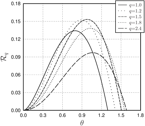
Figure 1: The relative quantity $\mathcal{R}_{q}$ versus $\theta$ for $s=1/2$, $n=3$, and five values of $q$, namely $q=1.0;1.2;1.5;1.8;2.4$. For each value of $q$, only positive values of $\mathcal{R}_{q}$ are shown.

On Fig. 1, we have shown violations of the $q$-entropic Leggett–Garg inequalities for the spin $s=1/2$ and the number $n=3$. The curves are related to the values $q=1.0;1.2;1.5;1.8;2.4$. The standard choice $q=1$ considered in Ref. uksr12 is included for comparison. We see that the curve maximum goes to larger values of $\theta$ with growth of $q$. There is some extension of the domain, for which $\mathcal{R}_{q}>0$. For $q>2.4$, however, such an extension becomes negligible. Nevertheless, the curves of Fig. 1 clearly show an utility of the $q$-entropic approach. In this regard, $q$-entropic inequalities of the Leggett–Garg type are similar to the $q$-entropic Bell inequalities derived in Ref. rastqic14 . Measured results of the experiment with fixed $\theta$ do violate the inequality $\mathcal{R}_{q}\leq 0$ for one values of $q$ and do not for other ones, including the standard case $q=1$. It is a manifestation of the following fact. Entropic Leggett–Garg inequalities give only necessary conditions that probabilistic models are compatible with the macrorealistic picture.

For larger values of $s$ or $n$, a similar situation is observed. Here, we refrain from presenting corresponding curves. Instead, we describe some significant points. The above mentioned properties of curves for different $q$ remain valid. In particular, there is some domain, in which $q$-entropic inequalities give advances in comparison with the standard case $q=1$. On the other hand, with growing $s$ and $n$ we have seen a decrease of this domain. It may be related with the following fact. As reported in Ref. uksr12 , both the strength and the range of violations reduce with the increase of spin value. We also recall that the considered situation corresponds to equidistant time intervals. For experiments with unequal time intervals, the $q$-entropic approach may give additional possibilities for analyzing data of tests of the Leggett–Garg type. Another question is related to detection inefficiencies.

Using the Shannon entropies, the writers of Ref. rchtf12 examined the Bell inequalities in the case of detection inefficiencies. For the $q$-entropic inequalities, this issue was studied in Ref. rastqic14 . We showed that the $q$-entropic approach can allow to reduce an amount of required detection efficiency. We shall now examine this question for restrictions of the Leggett–Garg type. In the considered example, we have the probability (39), whence

$$H_{q}(X_{k})=\ln_{q}(2s+1)\ .$$ (49)

Then the additional term (31) reads

$$\Delta_{q}(\eta) =(n-2)\Bigl{\{}\eta^{q}\bigl{(}\eta^{q}+2(1-\eta)^{q}-1\bigr{)}\ln_{q}(2s+1)\Bigr{.}$$

. $$+\bigl{(}\eta^{q}+(1-\eta)^{q}\bigr{)}h_{q}(\eta)\Bigr{\}}\ .$$ (50)

The characteristic quantity $\mathcal{C}_{q}$ is given by the numerator of Eq. (48). The $q$-entropic inequality (19) claims $\mathcal{C}_{q}\leq 0$. Using measured data, we will actually deal with the quantity (30). As was mentioned above, we must confide that the violating term $\eta^{2q}{\,}\mathcal{C}_{q}$ is sufficiently large in comparison with the additional term (50). To do so, we introduce their ratio

$$r_{q}(\eta):=\eta^{-2q}{\,}\mathcal{C}_{q}^{-1}\bigl{|}\Delta_{q}(\eta)\bigr{|}\ ,$$ (51)

which is restricted to the case $\mathcal{C}_{q}>0$. Let us consider this ratio in our case $s=1/2$ and $n=3$. We use $\theta=0.9$, when the strength of violations is large for several values of $q$ (see Fig. 1). We have calculated $r_{q}(\eta)$ versus $\eta$ for such values of $q$. With respect to $\eta$, we especially focus an attention on values, which are close to $1$ from below. For fixed $q$, the ratio $r_{q}(\eta)$ decreases with such $\eta$ almost linearly, up to the inefficiency-free value $r_{q}(1)=0$. Due to almost linear dependence, we can describe each case by the value (51) for some $\eta$, say, for $\eta=0.99$. Approximately, we use $r_{q}(\eta)\approx 10^{2}{\,}r_{q}(0.99){\,}(1-\eta)$ within a range of linear behavior. In Table 1, the value $r_{q}(0.99)$ is presented for $\theta=0.9$ and several values of $q$.

Table 1: The values of the ratio (51) for $\eta=0.99$ and several $q$ in the case $s=1/2$, $n=3$, and $\theta=0.9$.

$q$	1.0	1.1	1.2	1.4	1.6	1.8	2.0
$r_{q}(0.99)$	0.711	0.504	0.386	0.266	0.212	0.186	0.173
$q$	2.2	2.4	3.0	4.0	6.0	8.0	10.0
$r_{q}(0.99)$	0.167	0.165	0.174	0.208	0.330	0.587	1.364

In general, the required amount of efficiency seems to be very high. At the same time, the value $r_{q}(0.99)$ essentially depends on $q$. Initially, this value quickly decreases with $q>1$. It then becomes increasing for sufficiently large $q$. Among $q$-entropic inequalities of the Leggett–Garg type, the choice $q=2$ is convenient. First, both the strength and range of violations are significant. Second, the ratio (51) is small for $\eta>0.99$ (see Table 1). Third, properties of the $q$-entropies are mathematically simpler in the case $q=2$. We have already reported such reasons in Ref. rastqic14 , where $q$-entropic inequalities of the Bell type were obtained. Studying the CHSH and KCBS scenarios, the $q$-entropic Bell inequalities were shown to be expedient. Using $q$-entropic inequalities, we can also reach new possibilities for analyzing data of the Leggett–Garg tests. Leggett–Garg inequalities under decoherence also deserve theoretical studies. We hope to address this question in future investigations.

V Conclusions

We have formulated inequalities of the Leggett–Garg type in terms of the $q$-entropies. For all $q\geq 1$, such inequalities follow from the existence of some joint probability distribution for outcomes of measurements at different instants of time. It turned out that quantum mechanics predicts violations of an entire family of $q$-entropic inequalities of the Leggett–Garg type. We illustrated violations with the example of quantum spin systems. The spin-$s$ system has been prepared initially in the completely mixed state. Entropic Leggett–Garg inequalities give only necessary conditions that probabilistic models are compatible with the macrorealism in the broader sense. We showed that the presented inequalities allow to widen a class of situations, in which an incompatibility with the macrorealism can be checked. Both the strength and range of violations can be increased by adopting appropriate values of the entropic parameter $q$. We also formulated $q$-entropic inequalities of the Leggett–Garg type in the case of detection inefficiencies. If we use $q$-entropic inequalities, then the required amount of efficiency can somehow be reduced. In the sense of experimental testing, Leggett–Garg inequalities for quantum system in a dephasing environment are another important question pal10 ; xu11 . The presented formulation could be useful in analysis of recent experiments to test Leggett–Garg inequalities.

References

- (1) W. Heisenberg, Z. Phys. 43 (1927) 172.
- (2) J.S. Bell, Physics 1 (1964) 195.
- (3) A. Einstein, B. Podolsky, and N. Rosen, Phys. Rev. 47 (1935) 777.
- (4) D. Bohm, Quantum Theory, Englewood Cliffs, Prentice-Hall (1951).
- (5) J.A. Bergou and M. Hillery, Introduction to the Theory of Quantum Information Processing, New York, Springer (2013).
- (6) N.D. Mermin, Rev. Mod. Phys. 65 (1993) 803.
- (7) J.F. Clauser, M.A. Horne, A. Shimony, and R.A. Holt, Phys. Rev. Lett. 23 (1969) 880.
- (8) A. Aspect, P. Grangier, and G. Roger, Phys. Rev. Lett. 49 (1982) 91.
- (9) A. Aspect, J. Dalibard, and G. Roger, Phys. Rev. Lett. 49 (1982) 1804.
- (10) A. Zeilinger, Rev. Mod. Phys. 71 (1999) S288.
- (11) A.A. Klyachko, M.A. Can, S. Binicioǧlu, and A.S. Shumovsky, Phys. Rev. Lett. 101 (2008) 020403.
- (12) A.J. Leggett, Found. Phys. 33 (2003) 1469.
- (13) A.J. Leggett and A. Garg, Phys. Rev. Lett. 54 (1985) 857.
- (14) C. Emary, N. Lambert, and F. Nori, Rep. Prog. Phys. 77 (2013) 016001.
- (15) J. Dressel, C.J. Broadbent, J.C. Howell, and A.N. Jordan, Phys. Rev. Lett. 106 (2011) 040402.
- (16) V. Athalye, S.S. Roy, and T.S. Mahesh, Phys. Rev. Lett. 107 (2011) 130402.
- (17) H. Katiyar, A.S. Shukla, K.R.K. Rao, and T.S. Mahesh, Phys. Rev. A 87 (2013) 052102.
- (18) M. Barbieri, Phys. Rev. A 80 (2009) 034102.
- (19) D. Avis, P. Hayden, and M.M. Wilde, Phys. Rev. A 82 (2010) 030102(R).
- (20) M.M. Wilde and A. Mizel, Found. Phys. 42 (2012) 256.
- (21) S. Das, S. Aravinda, R. Srikanth, and D. Home, Europhys. Lett. 104 (2013) 60006.
- (22) J. Dressel and A.N. Korotkov, Phys. Rev. A 89 (2014) 012125.
- (23) A. Palacios-Laloy, F. Mallet, F. Nguyen, P. Bertet, D. Vion, D. Esteve, A.N. Korotkov, Nature Phys. 6 (2010) 442.
- (24) J.-S. Xu, C.-F. Li, X.-B. Zou, and G.-C. Guo, Sci. Rep. 1 (2011) 101.
- (25) N.S. Williams and A.N. Jordan, Phys. Rev. Lett. 100 (2008) 026804.
- (26) C. Emary, N. Lambert, and F. Nori, Phys. Rev. A 86 (2012) 235447.
- (27) D. Gangopadhyay, D. Home, and A.S. Roy, Phys. Rev. A 88 (2013) 022115.
- (28) S.L. Braunstein and C.M. Caves, Phys. Rev. Lett. 61 (1988) 662.
- (29) N.J. Cerf and C. Adami, Phys. Rev. A 55 (1997) 3371.
- (30) R. Chaves and T. Fritz, Phys. Rev. A 85 (2012) 032113.
- (31) P. Kurzyński, R. Ramanathan, and D. Kaszlikowski, Phys. Rev. Lett. 109 (2012) 020404.
- (32) A.E. Rastegin, Quantum Inf. Comput. 14 (2014) 0996.
- (33) R. Chaves, Phys. Rev. A 87 (2013) 022102.
- (34) A.R. Usha Devi, H.S. Karthik, Sudha, and A.K. Rajagopal, Phys. Rev. A 87 (2013) 052103.
- (35) C. Tsallis, J. Stat. Phys. 52 (1988) 479.
- (36) J. Havrda and F. Charvát, Kybernetika 3 (1967) 30.
- (37) M. Gell-Mann and C. Tsallis, eds., Nonextensive Entropy – Interdisciplinary Applications, Oxford, Oxford University Press (2004).
- (38) A. Rényi, On Measures of Entropy and Information, Proceedings of 4th Berkeley Symposium on Mathematical Statistics and Probability, University of California Press, Berkeley, CA (1961) 547.
- (39) I. Bengtsson and K. Życzkowski, Geometry of Quantum States: An Introduction to Quantum Entanglement, Cambridge, Cambridge University Press (2006)
- (40) Y.-X. Zhao and Z.-H. Ma, Commun. Theor. Phys. 48 (2007) 11.
- (41) A.E. Rastegin, Commun. Theor. Phys. 58 (2012) 819.
- (42) T.M. Cover and J.A. Thomas, Elements of Information Theory, New York, John Wiley & Sons (1991).
- (43) S. Furuichi, J. Math. Phys. 47 (2006) 023302.
- (44) A.E. Rastegin, Kybernetika 48 (2012) 242.
- (45) J. Kofler and C̆. Brukner, Phys. Rev. Lett. 101 (2008) 090403.
- (46) J. Kofler and C̆. Brukner, Phys. Rev. A 87 (2012) 052115.
- (47) L.C. Biedenharn and J.D. Louck, Angular Momentum in Quantum Physics, Reading, Addison-Wesley (1981).