Microscopic thin shell wormholes in magnetic Melvin universe

Abstract

We construct thin shell wormholes in the magnetic Melvin universe. It is shown that in order to make a TSW in the Melvin spacetime the radius of the throat can not be larger than $\frac{2}{B_{0}}$ in which $B_{0}$ is the magnetic field constant. We also analyze the stability of the constructed wormhole in terms of a linear perturbation around the equilibrium point. In our stability analysis we scan a full set of the Equation of States such as Linear Gas, Chaplygin Gas, Generalized Chaplygin Gas, Modified Generalized Chaplygin Gas and Logarithmic Gas. Finally we extend our study to the wormhole solution in the unified Melvin and Bertotti-Robinson spacetime. In this extension we show that for some specific cases, the local energy density is partially positive but the total energy which supports the wormhole is positive.

I Introduction

The magnetic Melvin universe (more appropriately the Bonnor-Melvin universe) Melvin is sourced by a beam of magnetic field parallel to the $z$-axis in the Weyl coordinates {$t,\rho,z,\varphi$}. The metric depends only on the radial coordinate $\rho$ which makes a typical case of cylindrical symmetry. It is a regular, non-black hole solution of the Einstein-Maxwell equations. Behaviour of the magnetic field is $B\left(\rho\right)\sim\rho$ (for $\rho\rightarrow 0$) and $B\left(\rho\right)\sim\frac{1}{\rho^{3}}$ (for $\rho\rightarrow\infty$). At radial infinity the magnetic field vanishes but spacetime is not flat. On the symmetry axis ($\rho=0$) the magnetic field vanishes; since the behaviour is same for $0\leqslant\left|z\right|<\infty$ the Melvin spacetime is not asymptotically flat also for $\left|z\right|\rightarrow\infty$. The magnetic field can be assumed strong enough to warp spacetime to the extent that it produces possible wormholes. Strong magnetic fields are available in magnetars (i.e. $B\sim 10^{15}G,$ while our Earth’s magnetic field is $B_{Earth}\sim 0.5G$), pulsars and other objects. Since creation of strong magnetic fields can be at our disposal in a laboratory - at least in very short time intervals - it is natural to raise the question whether wormholes can be produced in a magnetized superconducting environment. From this reasoning we aim to construct a thin-shell wormhole (TSW) in a magnetic Melvin universe. The method is an art of spacetime tailoring, i.e. cutting and pasting at a throat region under well-defined mathematical junction conditions. Some related papers can be found in TSWS for spherically symmetric bulk and in TSWC for cylindrically symmetric. The TSW is threaded by exotic matter which is taken for granted, and our principal aim is to search for the stability criteria for such a wormhole. Two cylindrically symmetric Melvin universes are glued at a hypersurface radius $\rho=a=$constant, which is endowed with surface energy-momentum to provide necessary support against the gravitational collapse. It turns out that in the Melvin spacetime the radial flare-out condition, i.e. $\frac{dg_{\varphi\varphi}}{da}>0$ is satisfied for a restricted radial distance, which makes a small scale wormhole. Specifically, this amounts to a throat radius $\rho=a<\frac{2}{\left|B_{o}\right|},$ so that for high magnetic fields the throat radius can be made arbitrarily small. This can be dubbed as a microscopic wormhole. As stated recently such small wormholes may host the quantum Einstein-Podolsky-Rosen (EPR) pair EPR . The throat is linearly perturbed in the radial distance and the resulting perturbation equation is obtained. The problem is reduced to a one-dimensional particle problem whose oscillatory behavior for an effective potential $V(a)$ about the equilibrium point is provided by $V^{\prime\prime}(a_{0})>0$. Given the Equation of State (EoS) on the hypersurface we plot the parametric stability condition $V^{\prime\prime}(a_{0})>0$ to determine the possible stable regions. Our samples of EoS consist of a Linear Gas, various forms of Chaplygin Gas and a Logarithmic gas. We consider TSW also in the recently found Melvin-Bertotti-Robinson magnetic universe MH1 . In the Bertotti-Robinson limit the wormhole is supported by total positive energy for any finite extension in the axial direction. For infinite extension the total energy reduces to zero, at least better than the total negative classical energy.

Organization of the paper is as follows. Construction of TSW from the magnetic Melvin spacetime is introduced in Sec. II. Stability of the TSW is discussed in Sec. III. Sec. IV discusses the consequences of small velocity perturbations. Section V considers TSW in Melvin-Bertotti-Robinson spacetime and Conclusion in Sec. VI completes the paper.

II Thin-shell wormhole in Melvin geometry

Let’s start with the Melvin magnetic universe spacetime Melvin in its axially symmetric form

$$ds^{2}=U\left(\rho\right)\left(-dt^{2}+d\rho^{2}+dz^{2}\right)+\frac{\rho^{2}}{U\left(\rho\right)}d\varphi^{2}$$ (1)

in which

$$U\left(\rho\right)=\left(1+\frac{B_{0}^{2}}{4}\rho^{2}\right)^{2}$$ (2)

where $B_{0}$ denotes the magnetic field constant. The Maxwell field two-form, however, is given by

$$\mathbf{F}=\frac{\rho B_{0}}{U\left(\rho\right)}d\rho\wedge d\varphi.$$ (3)

We note that the Melvin solution in Einstein-Maxwell theory does not represent a black hole solution. The solution is regular everywhere as seen from the Ricci scalar and Ricci sequence

$$R = 0$$ (4)

$$R_{\mu\nu}R^{\mu\nu} = \frac{4B_{0}^{4}}{U\left(\rho\right)^{8}}$$

as well as the Kretschmann scalar

$$\mathcal{K}=\frac{4B_{0}^{4}\left(3B_{0}^{4}\rho^{4}-24B_{0}^{2}\rho^{2}+80\right)}{U\left(\rho\right)^{8}}.$$ (5)

In BR , the general conditions which should be satisfied to have cylindrical wormhole possible are discussed. In brief, while the stronger condition implies that $\sqrt{g_{\varphi\varphi}}$ should take its minimum value at the throat, the weaker condition states that $\sqrt{g_{\varphi\varphi}g_{zz}}$ should be minimum at the throat. The stronger and weaker conditions are called radial flare-out and areal flare-out conditions respectively ES1 ; ES2 ; R . As we shall see in the sequel, in the case of TSW $\sqrt{g_{\varphi\varphi}}$ and $\sqrt{g_{\varphi\varphi}g_{zz}}$ should only be increasing function at the throat in radial flare-out and areal flare-out conditions. In the case of the Melvin spacetime,

$$\sqrt{g_{\varphi\varphi}}=\frac{\rho}{1+\frac{B_{0}^{2}}{4}\rho^{2}}$$ (6)

and

$$\sqrt{g_{\varphi\varphi}g_{zz}}=\rho.$$ (7)

One easily finds that areal flare-out condition is trivially satisfied and the radial flare-out condition requires $\rho<\frac{2}{B_{0}}$.  

Following Visser Visser , from the bulk spacetime (1) we cut two non-asymptotically flat copies $\mathcal{M}^{\pm}$ from a radius $\rho=a$ with $a>0$ and then we glue them at a hypersurface $\Sigma=\Sigma^{\pm}$ which is defined as $\mathcal{H}\left(\rho\right)=\rho-a\left(\tau\right)=0.$ In this way the resultant manifold is complete. At hypersurface $\Sigma$ the induced line element is given by

$$ds^{2}=-d\tau^{2}+U\left(a\right)dz^{2}+\frac{a^{2}}{U\left(a\right)}d\varphi^{2}$$ (8)

in which

$$-1=U\left(a\right)\left(-\dot{t}^{2}+\dot{\rho}^{2}\right)$$ (9)

where a dot stands for derivative with respect to the proper time $\tau$ on the hypersurface $\Sigma$. The Israel junction conditions which are the Einstein equations on the junction hypersurface read as ($8\pi G=1$)

$$k_{i}^{j}-k\delta_{i}^{j}=-S_{i}^{j},$$ (10)

in which $k_{i}^{j}=K_{i}^{j\left(+\right)}-K_{i}^{j\left(-\right)},$ $k=tr\left(k_{i}^{j}\right)$ and

$$K_{ij}^{\left(\pm\right)}=-n_{\gamma}^{\left(\pm\right)}\left(\frac{\partial^{2}x^{\gamma}}{\partial X^{i}\partial X^{j}}+\Gamma_{\alpha\beta}^{\gamma}\frac{\partial x^{\alpha}}{\partial X^{i}}\frac{\partial x^{\beta}}{\partial X^{j}}\right)_{\Sigma}$$ (11)

is the extrinsic curvature. Also the normal unit vector is defined as

$$n_{\gamma}^{\left(\pm\right)}=\left(\pm\left|g^{\alpha\beta}\frac{\partial\mathcal{H}}{\partial x^{\alpha}}\frac{\partial\mathcal{H}}{\partial x^{\beta}}\right|^{-1/2}\frac{\partial\mathcal{H}}{\partial x^{\gamma}}\right)_{\Sigma}$$ (12)

and $S_{i}^{j}=$diag$\left(-\sigma,P_{z},P_{\varphi}\right)$ is the energy momentum tensor on $\Sigma$. Explicitly we find,

$$n_{\gamma}^{\left(\pm\right)}=\pm\left(-\dot{a}U\left(a\right),U\left(a\right)\sqrt{\Delta},0,0\right)_{\Sigma},$$ (13)

in which $\Delta=\frac{1}{U\left(a\right)}+\dot{a}^{2}$. The non-zero components of the extrinsic curvature are found as

$$K_{\tau}^{\tau\left(\pm\right)}=\pm\frac{1}{\sqrt{\Delta}}\left(\ddot{a}+\frac{U^{\prime}}{U}\dot{a}^{2}+\frac{U^{\prime}}{2U^{2}}\right)$$ (14)

$$K_{z}^{z\left(\pm\right)}=\pm\frac{U^{\prime}}{2U}\sqrt{\Delta},$$ (15)

and

$$K_{\varphi}^{\varphi\left(\pm\right)}=\pm\left(\frac{1}{a}-\frac{U^{\prime}}{2U}\right)\sqrt{\Delta},$$ (16)

in which prime implies $\frac{\partial}{\partial a}$. Imposing the junction conditions Israel we find the components of the energy momentum tensor on the shell which are expressed as

$$\sigma=-\frac{2}{a}\sqrt{\Delta}$$ (17)

$$P_{z}=\frac{2\ddot{a}+\frac{2U^{\prime}}{U}\dot{a}^{2}+\frac{U^{\prime}}{U^{2}}}{\sqrt{\Delta}}+\left(\frac{2}{a}-\frac{U^{\prime}}{U}\right)\sqrt{\Delta},$$ (18)

and

$$P_{\varphi}=\frac{2\ddot{a}+\frac{2U^{\prime}}{U}\dot{a}^{2}+\frac{U^{\prime}}{U^{2}}}{\sqrt{\Delta}}+\frac{U^{\prime}}{U}\sqrt{\Delta}.$$ (19)

Having energy density on the shell, one may find the total exotic matter which supports the wormhole per unit $z$ by

$$\Omega=2\pi aU\left(a\right)\sigma$$ (20)

which is clearly exotic.

III Stability of the thin-shell wormhole against a linear perturbation

Recently, we have generalized the stability of TSWs in cylindrical symmetric bulks in MH2 . Here we apply the same method to the TSWs in Melvin universe. Similar to the spherical symmetric TSW, we start with the energy conservation identity on the shell which implies

$$\left(aS_{;j}^{ij}=\right)\frac{d}{d\tau}\left(a\sigma\right)+\left[\frac{aU^{\prime}}{2U}\left(P_{z}-P_{\varphi}\right)+P_{\varphi}\right]\frac{da}{d\tau}\\ =\frac{da}{d\tau}\frac{U^{\prime}}{U}\left(4-a\frac{U^{\prime}}{U}\right)\sqrt{\Delta}.$$ (21)

As we have shown in previous section the expressions given for surface energy density $\sigma$ and surface pressures $P_{z}$ and $P_{\varphi}$ are for a dynamic wormhole. This means that if there exists an equilibrium radius for the throat radius, say $a=a_{0},$ at this point $\dot{a}_{0}=0$ and $\ddot{a}_{0}=0$ and consequently the form of the surface energy density and pressure reduce to the static forms as

$$\sigma_{0}=-\frac{2}{a_{0}\sqrt{U_{0}}}$$ (22)

$$P_{z0}=\frac{2}{a_{0}\sqrt{U_{0}}}$$ (23)

and

$$P_{\varphi 0}=2\frac{U_{0}^{\prime}}{U_{0}\sqrt{U_{0}}}.$$ (24)

Let’s assume that after the perturbation the surface pressures are a general function of $\sigma$ which may be written as

$$P_{z}=\Psi\left(\sigma\right)$$ (25)

and

$$P_{\varphi}=\Phi\left(\sigma\right)$$ (26)

such that at the throat i.e. $a=a_{0}$, $\Psi\left(\sigma_{0}\right)=$ $P_{z0}$ and $\Phi\left(\sigma_{0}\right)=P_{\varphi 0}.$ From (17) one finds a one-dimensional type equation of motion for the throat

$$\dot{a}^{2}+V\left(a\right)=0$$ (27)

in which $V\left(a\right)$ is given by

$$V\left(a\right)=\frac{1}{U}-\left(\frac{a\sigma}{2}\right)^{2}.$$ (28)

Using the energy conservation identity (21), one finds

$$\left(a\sigma\right)^{\prime}=-\left[\frac{aU^{\prime}}{2U}\left(\Psi\left(\sigma\right)-\Phi\left(\sigma\right)\right)+\Phi\left(\sigma\right)\right]+\\ \frac{U^{\prime}}{U}\left(4-a\frac{U^{\prime}}{U}\right)\sqrt{\Delta},$$ (29)

which helps us to show that $V^{\prime}\left(a_{0}\right)=0$ and

$$V_{0}^{\prime\prime}=\frac{\left(2U_{0}+a_{0}U_{0}^{\prime}\right)\left[U_{0}^{\prime}\left(\Phi_{0}^{\prime}-\Psi_{0}^{\prime}\right)a_{0}-2U_{0}\Phi_{0}^{\prime}\right]}{2U_{0}^{3}a_{0}^{2}}-\\ \frac{U_{0}^{2}\left(2U_{0}^{\prime}-4a_{0}U_{0}^{\prime\prime}\right)+U_{0}\left(2U_{0}^{\prime\prime}U_{0}^{\prime}a_{0}^{2}+7a_{0}U_{0}^{\prime 2}\right)-3a_{0}^{2}U_{0}^{\prime 3}}{2U_{0}^{4}a_{0}}.$$ (30)

Note that a sub zero means that the corresponding quantity is evaluated at the equilibrium radius i.e., $a=a_{0}$. We also note that a prime denotes derivative with respect to its argument, for instance $\Psi_{0}^{\prime}=\left.\frac{\partial\Psi}{\partial\sigma}\right|_{\sigma=\sigma_{0}}$ while $U_{0}^{\prime}=\left.\frac{\partial U}{\partial a}\right|_{a=a_{0}}.$ Now, if we expand the equation of motion of the throat about $a=a_{0}$ we find (up to second order)

$$\ddot{x}+\omega^{2}x\tilde{=}0$$ (31)

in which $x=a-a_{0}$ and $\omega^{2}=\frac{1}{2}V^{\prime\prime}\left(a_{0}\right).$ This equation describes the motion of a harmonic oscillator provided $\omega^{2}>0$ which is the case of stability. If $\omega^{2}<0$ it implies that after the perturbation an exponential form fails to return back to its equilibrium point and therefore the wormhole is called unstable.

To conclude about the stability of the TSW in Melvin magnetic space we should examine the sign of $V^{\prime\prime}\left(a_{0}\right)$ and in any region where $V^{\prime\prime}\left(a_{0}\right)>0$ the wormhole is stable and in contrast if $V^{\prime\prime}\left(a_{0}\right)<0$ we conclude that the wormhole is unstable. From Eq. (30), we observe that this issue is identified with $a,$ $U_{0},$ $U_{0}^{\prime},$ $U_{0}^{\prime\prime}$ together with $\Phi_{0}^{\prime}$ and $\Psi_{0}^{\prime}.$ Since the form of $U\left(a\right)$ is known in order to examine the stability of the wormhole one should choose a specific EoS i.e. $\Psi\left(\sigma\right)$ and $\Phi\left(\sigma\right)$. In the following chapter we shall consider the well known cases of EoS which have been introduced in the literature. For each case we determine whether the TSW is stable or not.

III.1 Specific EoS

As we have already mentioned, in this chapter we go through the details of some specific EoS and the stability of the corresponding TSW.

III.1.1 Linear Gas (LG)

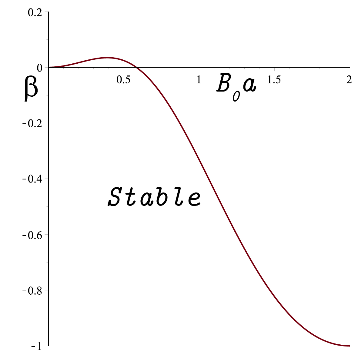
Figure 1: Stability of TSW supported by LG in terms of $a_{0}B_{0}$ and $\beta=\beta_{1}=\beta_{2}$. We note that the upper bound of $a_{0}B_{0}$ is chosen to be $2.$ This let $\frac{a^{2}}{f\left(a\right)}$ to remain an increasing function with respect to $a.$ This condition is needed to have a TSW possible in CS spacetime [5].

Our first choice of the EoS is a LG in which $\Psi^{\prime}\left(\sigma\right)=\beta_{1}$ and $\Phi^{\prime}\left(\sigma\right)=\beta_{2}$ with $\beta_{1}$ and $\beta_{2}$, two constant parameters related to the speed of sound in $z$ and $\varphi$ directions. We also find the form of $\Psi\left(\sigma\right)$ and $\Phi\left(\sigma\right)$ which are

$$\Psi\left(\sigma\right)=\beta_{1}\sigma+\Psi_{0}$$ (32)

and

$$\Phi\left(\sigma\right)=\beta_{2}\sigma+\Phi_{0}$$ (33)

with $\Psi_{0}$ and $\Phi_{0}$ as integration constants. We impose $\Psi\left(\sigma_{0}\right)=P_{z0}$ and $\Phi\left(\sigma_{0}\right)=P_{\varphi 0},$ which yields

$$\Psi_{0}=P_{z0}-\beta_{1}\sigma_{0}$$ (34)

and

$$\Phi_{0}=P_{\varphi 0}-\beta_{2}\sigma_{0}.$$ (35)

In the case with $\beta_{1}=$ $\beta_{2}=\beta$, we find that $\Psi$ and $\Phi$ are related as

$$\Psi-\Phi=P_{z0}-P_{\varphi 0}$$ (36)

but in general they are independent. In Fig. 1 we consider $\beta_{1}=$ $\beta_{2}=\beta$ and the resulting stable region with $V_{0}^{\prime\prime}>0$ is displayed.

III.1.2 Chaplygin Gas (CG)

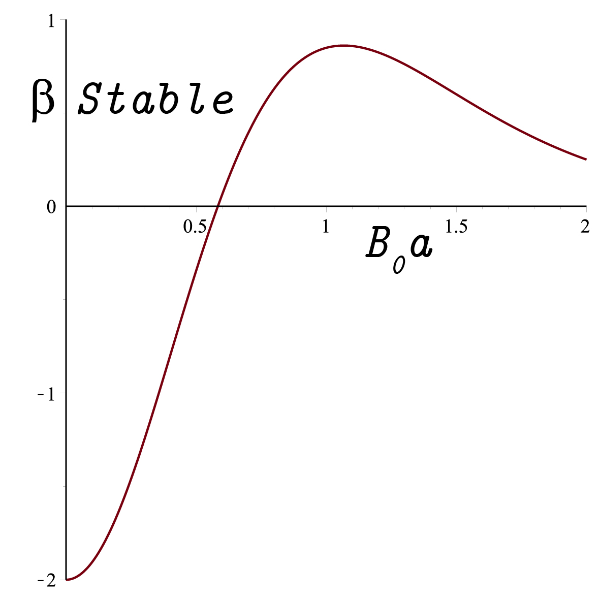
Figure 2: Stability of TSW supported by CG in terms of $a_{0}B_{0}$ and $\beta=\beta_{1}=\beta_{2}$.

Our second choice of the EoS is a CG. The form of $\Psi^{\prime}$ and $\Phi^{\prime}$ are given by

$$\Psi^{\prime}=\frac{\beta_{1}}{\sigma^{2}}\text{ and }\Phi^{\prime}=\frac{\beta_{2}}{\sigma^{2}}$$ (37)

in which $\beta_{1}$ and $\beta_{2}$ are two new positive constants. Furthermore, one finds

$$\Psi\left(\sigma\right)=-\frac{\beta_{1}}{\sigma}+\Psi_{0}$$ (38)

and

$$\Phi\left(\sigma\right)=-\frac{\beta_{2}}{\sigma}+\Phi_{0}$$ (39)

in which as before $\Psi_{0}$ and $\Phi_{0}$ are two integration constants. Imposing the equilibrium conditions $\Psi\left(\sigma_{0}\right)=P_{z0}$ and $\Phi\left(\sigma_{0}\right)=P_{\varphi 0}$ we find

$$\Psi_{0}=P_{z0}+\frac{\beta_{1}}{\sigma_{0}}$$ (40)

and

$$\Phi_{0}=P_{\varphi 0}+\frac{\beta_{2}}{\sigma_{0}}.$$ (41)

In Fig. 2 we plot the stability region of the TSW in terms of $\beta_{1}=$ $\beta_{2}=\beta$ and $B_{0}a.$ We note that setting $\beta_{1}=$ $\beta_{2}=\beta$ makes $\Psi$ and $\Phi$ dependent as in the LG case i.e., (36) but in general they are independent.

III.1.3 Generalized Chaplygin Gas (GCG)

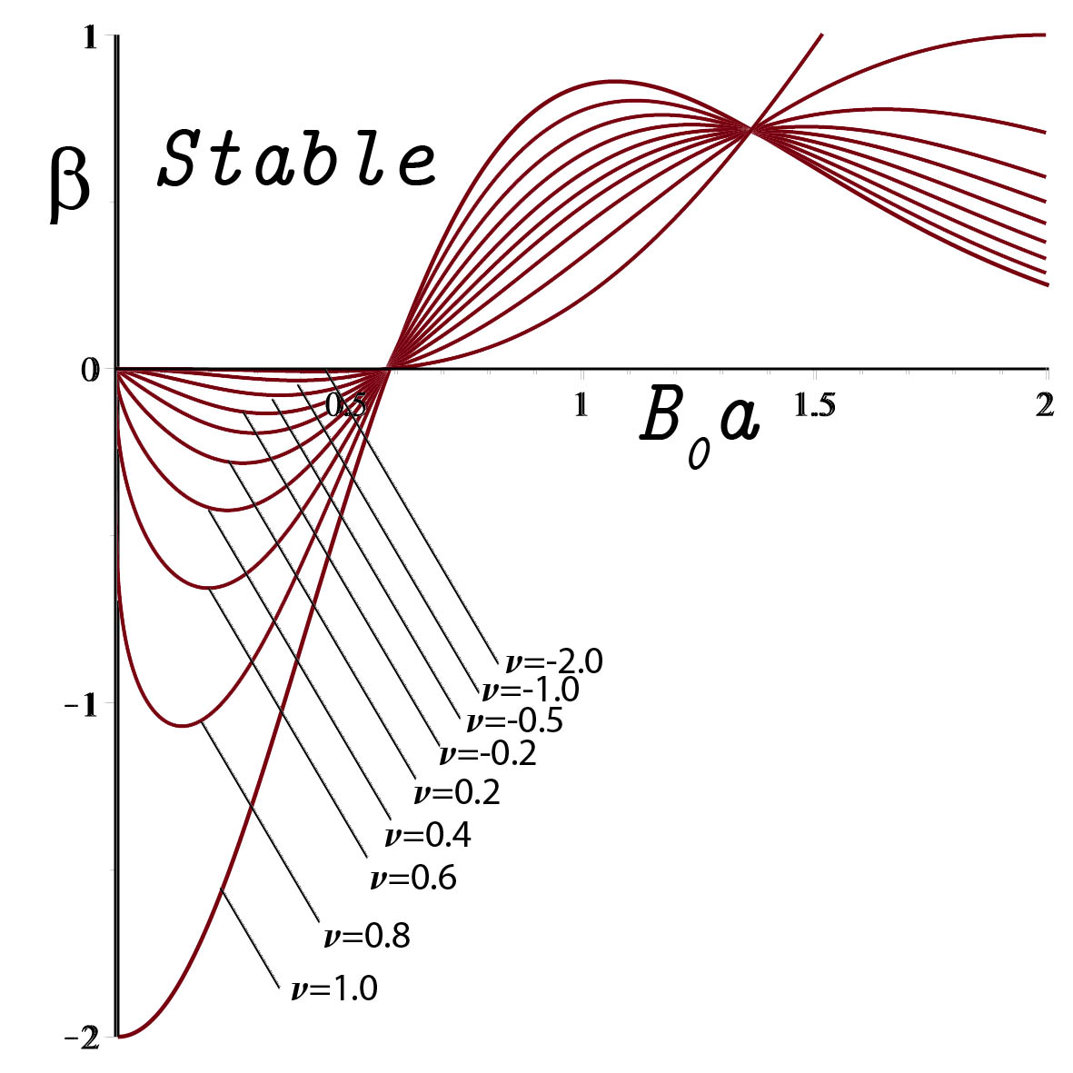
Figure 3: Stability of TSW supported by GCG in terms of $a_{0}B_{0}$ and $\beta=\beta_{1}=\beta_{2}$ with various value of $\nu.$ The stable region is noted.

After CG in this part we consider a GCG EoS which is defined as

$$\Psi^{\prime}=\frac{\beta_{1}}{\sigma\left|\sigma\right|^{\nu}}\text{ and }\Phi^{\prime}=\frac{\beta_{2}}{\sigma\left|\sigma\right|^{\nu}}$$ (42)

and consequently

$$\Psi\left(\sigma\right)=-\frac{\beta_{1}}{\nu\left|\sigma\right|^{\nu}}+\Psi_{0}$$ (43)

and

$$\Phi\left(\sigma\right)=-\frac{\beta_{2}}{\nu\left|\sigma\right|^{\nu}}+\Phi_{0}.$$ (44)

As before $\beta_{1}$ and $\beta_{2}$ are two new positive constants, $0<\nu\leq 1$ and $\Psi_{0}$ and $\Phi_{0}$ are integration constants. If we set $\beta_{1}=$ $\beta_{2}=\beta$ again $\Psi$ and $\Phi$ are not independent as Eq. (36). The equilibrium conditions imply

$$\Psi_{0}=P_{z0}+\frac{\beta_{1}}{\nu\left|\sigma_{0}\right|^{\nu}}$$ (45)

while

$$\Phi_{0}=P_{\varphi 0}+\frac{\beta_{2}}{\nu\left|\sigma_{0}\right|^{\nu}}.$$ (46)

In Fig. 3 we show the effect of the additional freedom i.e., $\nu$ in the stability of the corresponding TSW. We note that although in the standard definition of the GCG one has to consider $0<\nu\leq 1$ in our figure we also considered beyond this limit.

III.1.4 Modified Generalized Chaplygin Gas (MGCG)

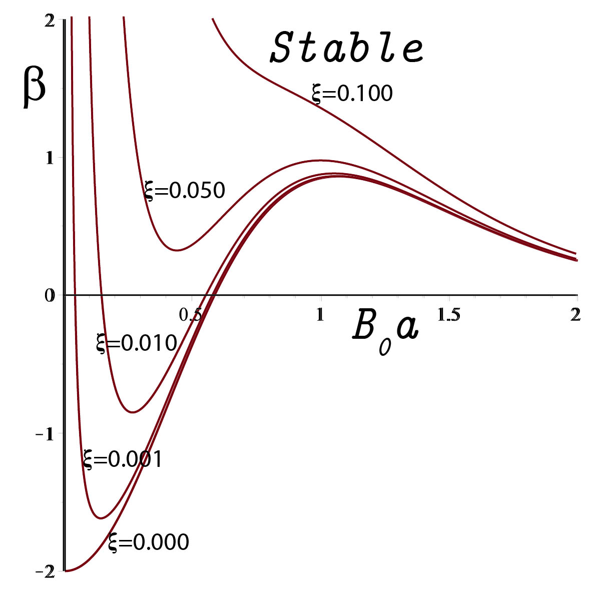
Figure 4: Stability of TSW supported by MGCG in terms of $a_{0}B_{0}$ and $\beta=\beta_{1}=\beta_{2}$. The different curves are for different values of $\xi=\xi_{1}=\xi_{2}$ and $\nu$ is chosen to be $\nu=1.$

Another step toward further generalization is to combine the LG and the GCG. This is called MGCG and the form of the EoS may be written as

$$\Psi^{\prime}=\xi_{1}+\frac{\beta_{1}}{\sigma\left|\sigma\right|^{\nu}}\text{ and }\Phi^{\prime}=\xi_{2}+\frac{\beta_{2}}{\sigma\left|\sigma\right|^{\nu}}.$$ (47)

Herein, $\beta_{1}>0$, $\beta_{2}>0$, $\xi_{1}$ and $\xi_{2}$ are constants and $0<\nu\leq 1.$ The form of $\Psi$ and $\Phi$ can be found as

$$\Psi\left(\sigma\right)=\xi_{1}\sigma-\frac{\beta_{1}}{\nu\left|\sigma\right|^{\nu}}+\Psi_{0}$$ (48)

and

$$\Phi\left(\sigma\right)=\xi_{2}\sigma-\frac{\beta_{2}}{\nu\left|\sigma\right|^{\nu}}+\Phi_{0}.$$ (49)

As before $\Psi_{0}$ and $\Phi_{0}$ are integration constants which can be identified by imposing the similar equilibrium conditions i.e., $\Psi\left(\sigma_{0}\right)=P_{z0}$ and $\Phi\left(\sigma_{0}\right)=P_{\varphi 0}.$ After that we find

$$\Psi_{0}=P_{z0}+\frac{\beta_{1}}{\nu\left|\sigma_{0}\right|^{\nu}}-\xi_{1}\sigma_{0}$$ (50)

and

$$\Phi_{0}=P_{\varphi 0}+\frac{\beta_{2}}{\nu\left|\sigma_{0}\right|^{\nu}}-\xi_{2}\sigma_{0}.$$ (51)

In Fig. 4 we plot the stability region of the TSW supported by the MGCG with additional arrangements as $\xi_{1}=\xi_{2}=\xi$ and $\beta_{1}=$ $\beta_{2}=\beta.$ We again comment that these make $\Psi$ and $\Phi$ dependent while in general they are independent. In Fig. 4 specifically we show the effect of the additional freedom to the GCG, i.e., $\xi$ in a frame of $\beta$ and $B_{0}a.$

III.1.5 Logarithmic Gas (LogG)

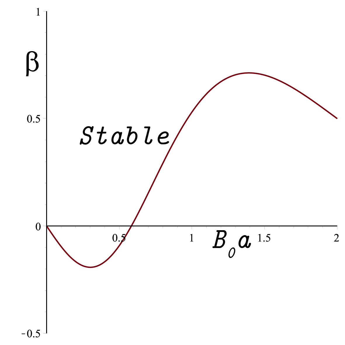
Figure 5: Stability of TSW supported by LogG in terms of $a_{0}B_{0}$ and $\beta=\beta_{1}=\beta_{2}$. We note that the upper bound of $a_{0}B_{0}$ is chosen to be $2.$

Finally we consider the LogG with

$$\Psi^{\prime}=-\frac{\beta_{1}}{\sigma}\text{ and }\Phi^{\prime}=-\frac{\beta_{2}}{\sigma}$$ (52)

where $\beta_{1}>0$ and $\beta_{2}>0$ are two positive constants. The EoS are given by

$$\Psi=-\beta_{1}\ln\left|\frac{\sigma}{\sigma_{0}}\right|+\Psi_{0}\text{ and }\Phi=-\beta_{1}\ln\left|\frac{\sigma}{\sigma_{0}}\right|+\Phi_{0}$$ (53)

in which the $\beta_{1}\ln\left|\sigma_{0}\right|+\Psi_{0}$ and $\beta_{2}\ln\left|\sigma_{0}\right|+\Phi_{0}$ are integration constants. Imposing the equilibrium conditions one finds $\Psi_{0}=P_{z0}$ and $\Phi_{0}=P_{\varphi 0}.$ In Fig. 5 we plot the stability region in terms of $\beta_{1}=$ $\beta_{2}=\beta$ versus $B_{0}a.$

IV Small velocity perturbation

In the previous chapter we have considered a linear perturbation around the equilibrium point of the throat. As we have considered above, the EoS of the fluid on the thin shell after the perturbation had no relation with its equilibrium state. However, by setting $\beta_{1}=\beta_{2}$ in our analysis in previous chapter, implicitly we accepted that $\Psi-\Phi=P_{z}-P_{\varphi}$ does not change in time, a restriction that is physically acceptable.

In this chapter we consider the EoS of the TSW after the perturbation same as its equilibrium point. This in fact means that the time evolution of the throat is slow enough that any intermediate step between the initial point and a certain final point can be considered as another equilibrium point (or static). Quantitatively it means that $\frac{P_{z}}{\sigma}=-1$ (same as $\frac{P_{z0}}{\sigma_{0}}=-1$) and $\frac{P_{\varphi}}{\sigma}=-a\frac{U^{\prime}}{U}$ (same as$\frac{P_{\varphi 0}}{\sigma_{0}}=-a_{0}\frac{U_{0}^{\prime}}{U_{0}}$) and consequently, from (17), (18) and (19), we find a single second order differential equation which may be written as

$$2\ddot{a}+\frac{U^{\prime}}{U}\dot{a}^{2}=0.$$ (54)

This equation gives the exact motion of the throat after the perturbation. (We note once more that the process of time evolution is considered with small velocity). This equation can be integrated to obtain

$$\dot{a}=\dot{a}_{0}\sqrt{\frac{U_{0}}{U}}.$$ (55)

A second integration with the exact form of $U,$ yields

$$a\left(1+\frac{B_{0}^{2}}{12}a^{2}\right)=a_{0}\left(1+\frac{B_{0}^{2}}{12}a_{0}^{2}\right)+\dot{a}_{0}\sqrt{U_{0}}\left(\tau-\tau_{0}\right).$$ (56)

The motion of the throat is under a negative force per unit mass which is position and velocity dependent. As it is clear from the expression of $\dot{a},$ the magnitude of velocity is always positive and it never vanishes. This means that the motion of the throat is not oscillatory but builds up in the same direction after perturbation. Also from (56) we see that in proper time if $\dot{a}_{0}>0,$ $a$ goes to infinity and when $\dot{a}_{0}<0,$ $a$ goes to zero. In both cases the particle-like motion does not return to its initial position $a=a_{0}$. These mean that the TSW is not stable under small velocity perturbations.

V TSW in Unified Bertotti-Robinson and Melvin spacetimes

Recently two of us found a new solution to Einstein-Maxwell equations which represents unified Bertotti-Robinson and Melvin spacetimes MH1 whose line element is given by

$$ds^{2}=-e^{2u}dt^{2}+e^{-2u}\left[e^{2\kappa}\left(d\rho^{2}+dz^{2}\right)+\rho^{2}d\varphi^{2}\right]$$ (57)

where

$$e^{u}=F=\lambda_{0}\left[\sqrt{\rho^{2}+z^{2}}\cosh\left(\frac{B_{0}}{\lambda_{0}}\ln\rho\right)-z\sinh\left(\frac{B_{0}}{\lambda_{0}}\ln\rho\right)\right],$$ (58)

and

$$e^{\kappa}=\frac{F^{2}}{\left(\rho^{2}+z^{2}\right)}\left[\frac{\rho^{1+\frac{B_{0}}{2\lambda_{0}}}}{z+\sqrt{\rho^{2}+z^{2}}}\right]^{\frac{2B_{0}}{\lambda_{0}}}.$$ (59)

Herein $\lambda_{0}$ and $B_{0}$ are two essential parameters of the spacetime which are related to the magnetic field of the system and the topology of the spacetime. The magnetic potential of the spacetime is given by

$$A_{\mu}=\Phi\left(\rho,z\right)\delta_{\mu}^{\varphi}$$ (60)

in which

$$\Phi_{\rho}\left(\rho,z\right)=\rho e^{-2u}\psi_{z}$$ (61)

and

$$\Phi_{z}\left(\rho,z\right)=-\rho e^{-2u}\psi_{\rho}$$ (62)

with

$$\psi=\lambda_{0}\left[\sqrt{\rho^{2}+z^{2}}\right]+B_{0}z.$$ (63)

The standard method of making TSW implies that $\mathcal{H}\left(\rho\right)=\rho-a\left(\tau\right)=0$ is the timelike hypersurface where the throat is located at and the line element on the shell reads

$$ds^{2}=-d\tau^{2}+e^{-2u\left(a,z\right)}\left[e^{2\kappa\left(a,z\right)}dz^{2}+a^{2}d\varphi^{2}\right].$$ (64)

The normal $4-$vector to the shell is found to be

$$n_{\gamma}^{\left(\pm\right)}=\pm\left(-\dot{a}e^{\kappa},e^{2\left(\kappa-u\right)}\sqrt{\Delta},0,0\right)_{\Sigma},$$

with $\Delta=\left(e^{2\left(u-\kappa\right)}+\dot{a}^{2}\right)$ and the non-zero elements of the extrinsic curvature tensor become

$$K_{\tau}^{\tau\left(\pm\right)}=\pm\left[\frac{\ddot{a}+\left(\kappa^{\prime}-u^{\prime}\right)\dot{a}^{2}}{\sqrt{\Delta}}+u^{\prime}\sqrt{\Delta}\right],$$ (65)

$$K_{z}^{z\left(\pm\right)}=\mp\left(u^{\prime}-\kappa^{\prime}\right)\sqrt{\Delta},$$ (66)

and

$$K_{\varphi}^{\varphi\left(\pm\right)}=\mp\left(u^{\prime}-\frac{1}{a}\right)\sqrt{\Delta}.$$ (67)

Upon the Israel junction conditions, one finds

$$\sigma=2\sqrt{\Delta}\left(2u^{\prime}-\kappa^{\prime}-\frac{1}{a}\right),$$ (68)

$$P_{z}=2\left[\frac{\ddot{a}+\left(\kappa^{\prime}-u^{\prime}\right)\dot{a}^{2}}{\sqrt{\Delta}}+\frac{1}{a}\sqrt{\Delta}\right]$$ (69)

and

$$P_{\varphi}=2\left[\frac{\ddot{a}+\left(\kappa^{\prime}-u^{\prime}\right)\dot{a}^{2}}{\sqrt{\Delta}}+\kappa^{\prime}\sqrt{\Delta}\right].$$ (70)

The results given above can be used to find the $\sigma_{0}$, $P_{z0}$ and $P_{\varphi 0}$ at the equilibrium radius $a=a_{0}$ i.e.,

$$\sigma_{0}=\left.2e^{\left(u-\kappa\right)}\left(2u^{\prime}-\kappa^{\prime}-\frac{1}{a}\right)\right|_{a=a_{0}},$$ (71)

$$P_{z0}=\left.\frac{2}{a}e^{\left(u-\kappa\right)}\right|_{a=a_{0}}$$ (72)

and

$$P_{\varphi 0}=\left.2\kappa^{\prime}e^{\left(u-\kappa\right)}\right|_{a=a_{0}}.$$ (73)

Next, we use the exact form of $\kappa$ and $u$ to find the energy density of the shell which can be written as

$$\sigma_{0}=\frac{2a_{0}}{a_{0}^{2}+z^{2}}-\frac{\left(\epsilon+1\right)^{2}}{a_{0}}+\frac{2\epsilon a_{0}}{\sqrt{a_{0}^{2}+z^{2}}\left(z+\sqrt{a_{0}^{2}+z^{2}}\right)}$$ (74)

in which $\epsilon=\frac{B_{0}}{\lambda_{0}}.$ To analyze the sign of $\sigma_{0}$ we introduce $\zeta=\frac{z}{a_{0}}$ and rewrite the latter equation as

$$a_{0}\sigma=-\left(1+\epsilon\right)^{2}+\frac{2\left(\zeta+\left(1+\epsilon\right)\sqrt{1+\zeta^{2}}\right)}{\left(1+\zeta^{2}\right)\left(\zeta+\sqrt{1+\zeta^{2}}\right)}.$$ (75)

One of the interesting case is when we set $\epsilon=-1$ which yields

$$a_{0}\sigma_{0}=\frac{2\zeta}{\left(1+\zeta^{2}\right)\left(\zeta+\sqrt{1+\zeta^{2}}\right)}.$$ (76)

This is positive for $\zeta>0$ ($z>0$), negative for $\zeta<0$ ($z<0$) and zero for $\zeta=0$ ($z=0$). Another interesting case is when we set $\epsilon=0$ which is the BR limit of the general solution (57-59). In this setting we find

$$a_{0}\sigma_{0}=\frac{2}{1+\zeta^{2}}-1$$ (77)

which is positive for $\left|\zeta\right|<1.$ In Fig. 6 we plot the region on which $a_{0}\sigma_{0}\geq 0$ in terms of $\epsilon$ and $\zeta.$ To find the total energy of the shell we use

$$\Omega=\int_{0}^{2\pi}\int_{-\infty}^{+\infty}\int_{0}^{\infty}\sigma_{0}\delta\left(\rho-a_{0}\right)\sqrt{-g}d\rho dzd\varphi$$ (78)

which after some manipulation becomes

$$\Omega=2\pi\int_{-\infty}^{+\infty}\sigma_{0}a_{0}e^{2\left(\kappa_{0}-u_{0}\right)}dz.$$ (79)

in which $\kappa_{0}=\left.\kappa\right|_{a=a_{0}}$ and $u_{0}=\left.u\right|_{a=a_{0}}.$

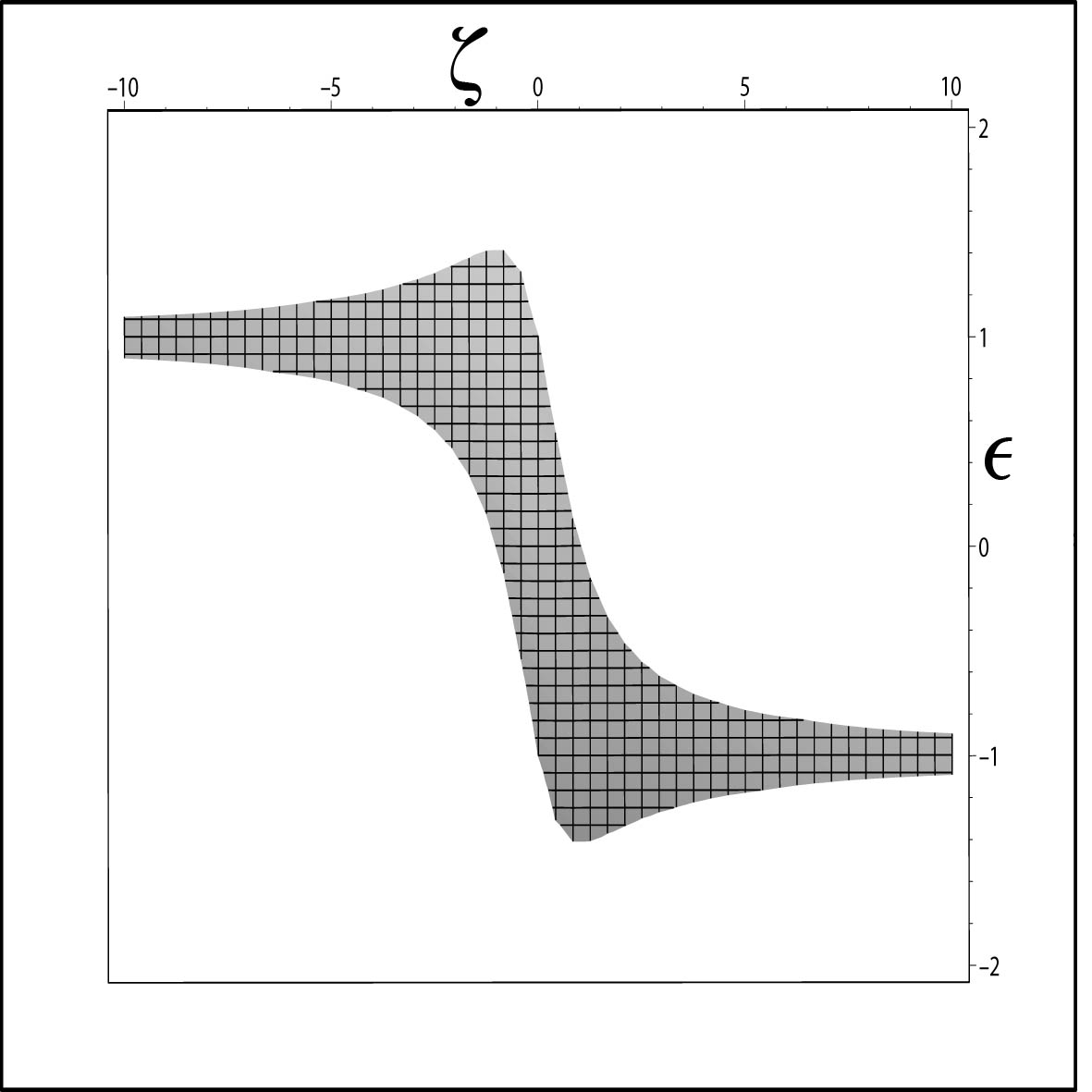
Figure 6: $a_{0}\sigma_{0}$ versus $\epsilon$ and $\zeta.$ The shaded region in the region on which $a_{0}\sigma_{0}$ is positive.

Upon some further manipulation we arrive at

$$\frac{\Omega}{2\pi\lambda_{0}^{2}a_{0}^{2\epsilon^{2}-1}}=\\ \int_{-\infty}^{\infty}\left[\frac{2\left(\zeta+\left(1+\epsilon\right)\sqrt{1+\zeta^{2}}\right)}{\left(1+\zeta^{2}\right)^{3}\left(\zeta+\sqrt{1+\zeta^{2}}\right)}-\frac{\left(1+\epsilon\right)^{2}}{\left(1+\zeta^{2}\right)^{2}}\right]\\ \frac{\left(\sqrt{1+\zeta^{2}}\cosh\left(\epsilon\ln a_{0}\right)-\zeta\sinh\left(\epsilon\ln a_{0}\right)\right)^{2}}{\left(\zeta+\sqrt{1+\zeta^{2}}\right)^{4\epsilon}}d\zeta.$$ (80)

Although this integral can not be evaluated explicitly for arbitrary $\epsilon$ at least for $\epsilon=0$ it gives

$$\Omega=\lim_{R\rightarrow\infty}\frac{4\pi\lambda_{0}^{2}R}{a_{0}\left(1+R^{2}\right)}$$ (81)

which is positive. Obviously this limit (i.e. $\epsilon=0$) corresponds to the Bertotti-Robinson limit of the general solution in which for $R<\infty$ construction of a TSW with a positive total energy becomes possible.

VI Conclusion

A large class of stable TSW solutions is found by employing the magnetic Melvin universe through the cut-and-paste technique. The Melvin spacetime is a typical cylindrically symmetric, regular solution of the Einstein-Maxwell equations. Herein the throat radius of the TSW is confined by a strong magnetic field, for this reason we phrase them as microscopic wormholes. Being regular its construction can be achieved by a finite energy. It has recently been suggested that the mysterious EPR particles may be connected through a wormhole Sus . From this point of view the magnetic Melvin wormhole may be instrumental to test such a claim. We have applied radial, linear perturbation to the throat radius of the TSW in search for stability regions. In such perturbations we observed that the initial radial speed must be chosen zero in order to attain a stable TSW. Different perturbations may cause collapse of the wormhole. As the material on the throat we have adopted various equations of states, ranging from an ordinary linear / logarithmic gas to a Chaplygin gas. The repulsive support derived from such sources gives life to the TSW against the gravitational collapse. Besides pure Melvin case we have also considered TSW in the magnetic universe of unified Melvin and Bertotti-Robinson spacetimes. The pure Bertotti-Robinson TSW has positive total energy for each finite axial length ($R<\infty$). The energy becomes zero when the cut-off length $R\rightarrow\infty.$

References

• (1) M. A. Melvin, Phys. Lett. 8, 65 (1964); W. B. Bonnor, Proc. Phys. Soc. London Sect. A 67, 225 (1954); D. Garfinkle and E. N. Glass, Classical Quantum Gravity 28, 215012 (2011).
• (2) M. Visser, Phys. Rev. D 39, 3182 (1989); M. Visser, Nucl. Phys. B 328, 203 (1989); P. R. Brady, J. Louko and E. Poisson, Phys. Rev. D 44, 1891 (1991); E. Poisson and M. Visser, Phys. Rev. D 52, 7318 (1995); M. Ishak and K. Lake, Phys. Rev. D 65, 044011 (2002); C. Simeone, Int. Jou. of Mod. Phys. D 21, 1250015 (2012); F. S. N. Lobo, Phys. Rev. D 71, 124022 (2005); E. F. Eiroa and C. Simeone, Phys. Rev. D 71, 127501 (2005); E. F. Eiroa, Phys. Rev. D 78, 024018 (2008); F. S. N. Lobo and P. Crawford, Class. Quantum Grav. 22, 4869 (2005); S. H. Mazharimousavi, M. Halilsoy and Z. Amirabi, Phys. Lett. A 375, 3649 (2011); M. Sharif and M. Azam, Eur. Phys. J. C 73, 2407 (2013); M. Sharif and M. Azam, Eur. Phys. J. C 73, 2554 (2013); S. H. Mazharimousavi and M. Halilsoy, Eur. Phys. J. C 73, 2527 (2013).
• (3) E. F. Eiroa and C. Simeone, Phys. Rev. D 70, 044008 (2004); M. Sharif and M. Azam, JCAP 04, 023 (2013); E. Rubín de Celis, O. P. Santillan and C. Simeone, Phys. Rev. D 86, 124009 (2012); C. Bejarano, E. F. Eiroa and C. Simeone, Phys. Rev. D 75, 027501 (2007); K. A. Bronnikov, V. G. Krechet and J. P. S. Lemos, Phys. Rev. D 87, 084060 (2013); M. G. Richarte, Phys. Rev. D 87, 067503 (2013); Z. Amirabi, M. Halilsoy and S. H. Mazharimousavi, Phys. Rev. D 88, 124023 (2013).
• (4) A. Einstein, B Podolsky and N. Rosen, Phys. Rev. 47, 777 (1935).
• (5) S. H. Mazharimousavi and M. Halilsoy, Phys. Rev. D 88, 064021 (2013).
• (6) K. A. Bronnikov and J. P. S. Lemos, Phys. Rev. D 79, 104019 (2009).
• (7) E. F. Eiroa and C. Simeone, Phys. Rev. D 81, 084022 (2010).
• (8) E. F. Eiroa and C. Simeone, Phys. Rev. D 82, 084039 (2010).
• (9) M. G. Richarte, Phys. Rev. D 88, 027507 (2013).
• (10) M. Visser, Phys. Rev. D 39, 3182 (1989); M. Visser, Nucl. Phys. B 328, 203 (1989).
• (11) W. Israel, Nuovo Cimento 44B, 1 (1966); V. de la Cruzand W. Israel, Nuovo Cimento 51A, 774 (1967); J. E. Chase, Nuovo Cimento 67B, 136. (1970); S. K. Blau, E. I. Guendelman, and A. H. Guth, Phys. Rev. D 35, 1747 (1987); R. Balbinot and E. Poisson, Phys. Rev. D 41, 395 (1990).
• (12) S. Habib Mazharimousavi, M. Halilsoy and Z. Amirabi, Phys. Rev. D (2014) in press, arXiv:1403.2861.
• (13) J. Maldacena and L. Susskind, arXiv:1306.0533 ”Cool horizons for entangled black holes”.