Parameter estimation of neutron star-black hole binaries using an advanced gravitational-wave detector network: Effects of the full post-Newtonian waveform

Abstract

We investigate the effects of using the full waveform (FWF) over the conventional restricted waveform (RWF) of the inspiral signal from a coalescing compact binary system in extracting the parameters of the source, using a global network of second generation interferometric detectors. We study a hypothetical population of (1.4-10)$M_{\odot}$ neutron star-black hole (NS-BH) binaries (uniformly distributed and oriented in the sky) by employing the full post-Newtonian waveforms, which not only include contributions from various harmonics other than the dominant one (quadrupolar mode) but also the post-Newtonian amplitude corrections associated with each harmonic, of the inspiral signal expected from this system. It is expected that the GW detector network consisting of the two LIGO detectors and a Virgo detector will be joined by KAGRA (a Japanese detector) and by proposed LIGO-India. We study the problem of parameter estimation with all 16 possible detector configurations. Comparing medians of error distributions obtained using FWFs with those obtained using RWFs (which only include contributions from the dominant harmonic with Newtonian amplitude) we find that the measurement accuracies for luminosity distance and the cosine of the inclination angle improve almost by a factor of 1.5-2 depending upon the network under consideration. We find that this improvement can be attributed to the presence of additional inclination angle dependent terms, which appear in the amplitude corrections to various harmonics, which break the strong degeneracy between the luminosity distance and inclination angle. Although the use of FWF does not improve the source localization accuracy much, the global network consisting of five detectors will improve the source localization accuracy by a factor of 4 as compared to the estimates using a three-detector LIGO-Virgo network for the same waveform model.

I Introduction

Coalescing compact binary (CCB) systems, composed of NSs and/or stellar mass BHs, are among the prime targets for the second generation of GW detectors such as advanced LIGO Harry and LIGO Scientific Collaboration (2010) and advanced Virgo avi . On the other hand, the proposed space-based detector eLISA Amaro-Seoane et al. (2012) shall be primarily looking at GW signals from super massive BHs. In addition, although there are no observational evidences for the existence of CCBs with intermediate mass BHs (with masses of few tens to few hundred solar masses), if at all such systems exist they should be observed by advanced ground-based detectors (see Pitkin et al. (2011) for a review on detection of GW sources from ground and space). The GW observation of stellar/intermediate mass CCB systems in advanced GW detectors will not only provide the first direct evidence for the existence of GWs but also will reveal a great deal of information about the source properties which cannot be accessed through conventional electromagnetic observations. Hence, apart from the problem of detection one is interested in estimating the parameters which characterize the source. In the case of ground-based detectors, in general one would have a situation when the GW signal is completely buried in the noise. Hence, in order to be able to detect or to extract parameters of the source one employs data analysis techniques such as matched filtering Helström (1968); Thorne (1987); Schutz (1989), which in turn requires accurate modeling of the dynamics of sources emitting the signal. This has led to the development of many analytical and numerical techniques which are used to model various stages of CCB evolution, namely, the early inspiral phase, the late inspiral, the merger phase and the final ringdown phase. For instance, the early inspiral phase can be very well modeled using approximation schemes in General Relativity (GR) such as the post-Newtonian (PN) approximation Blanchet (2006). The late inspiral and merger phase can be computed by using Numerical Relativity Pretorius (2007) whereas the final ringdown phase can be accurately modeled using black hole perturbation theory Sasaki and Tagoshi (2003).

Although, in general it is believed that at the time of their formation all CCB systems possess eccentric orbits, it is reasonable to assume that in late stages of their evolution (this is precisely the stage when signals would be visible in earth-bound detectors), their orbits would become circular due to radiation reaction Peters (1964). During this phase the signal from a nonspinning CCB can be approximated by a template whose frequency and amplitude steadily increases until the last stable orbit is reached. The phase Blanchet et al. (1995, 2002, 2004) and amplitude Blanchet et al. (1996); Arun et al. (2004); Kidder et al. (2007); Blanchet et al. (2008) of GW signals from CCBs in this stage has been computed to very high accuracies using the post-Newtonian approximations in GR. Further, the fact that the amplitude of the signal in this phase varies much more slowly as compared to the phase of the signal and also because most of the signal power is contained in the dominant harmonic (quadrupolar mode), it seems reasonable to approximate the signal to a template which neglects contributions from harmonics other than the dominant one and various post-Newtonian amplitude corrections associated with each harmonic. A waveform obtained in this fashion is called the restricted waveform (RWF) and contains only the dominant harmonic at twice the orbital frequency, with phase which includes all the PN corrections to the leading phase term but only the Newtonian amplitude. Note that modes other than the dominant one are suppressed as they contribute to the waveform at a higher post-Newtonian order. In the light of this argument we refer these additional modes together with the higher order post-Newtonian corrections to the amplitude of the dominant harmonics as subdominant modes and would follow this terminology in rest of the paper. It has been argued in a number of investigations that RWFs are good enough as far as the detection of low mass binaries (M$<$10$M_{\odot}$) are concerned (see e.g. Van Den Broeck and Sengupta (2007)). Even CCBs as massive as 25$M_{\odot}$ can be detected using template bank constructed using restricted waveform approximation of the inspiral signals, however, the efficiency of extracting parameters reduces as the mass of the binary increases (see the discussion in Ref. Farr et al. (2009)). It was discussed in the case of single ground-based detectors Van Den Broeck (2006); Van Den Broeck and Sengupta (2007) and in the case of space-based detector LISA Arun et al. (2007) that the mass reach of GW detectors can be significantly increased by including contributions from subdominant harmonics. Such a waveform which includes contributions from various subdominant harmonics and the post-Newtonian amplitude corrections associated with each harmonic is refer to as the full waveform (FWF). Although, as we move towards the higher mass end, even subdominant harmonics fail to penetrate the frequency band where the detector is most sensitive. In that case it becomes important to include the contributions from the merger phase of the binary evolution.

A recent work by Capano et al. Capano et al. (2013) suggests that, inspiral-merger-ringdown (IMR) waveforms based on just the contributions from dominant harmonic will be sufficient for detecting signals from binaries with total mass up to 360$M_{\odot}$. However, it was also mentioned that, for systems with total mass $>100M_{\odot}$ and with mass ratios $>4$, indeed the sensitivity of the search improves if the waveform includes contributions from subdominant modes . Another recent study based purely on numerical waveforms Pekowsky et al. (2012) suggests that with the inclusion of subdominant modes of the waveform the detection volume can be significantly increased (by about 30%) as compared to what could be achieved by using waveforms based on the RWF approximation of the inspiral signal. Some of the previous studies showed that that the inclusion of subdominant modes in the model of the GW signal not only improves the mass-reach and the detection rates of future GW detectors but also provides a more powerful template to match with the signal in order to extract the parameters of the source accurately in context of single ground based detectors Sintes and Vecchio (2000); Van Den Broeck and Sengupta (2007); Littenberg et al. (2013) and in the case of space-based LISA Sintes and Vecchio (2000); Moore and Hellings (2002); Hellings and Moore (2003); Arun et al. (2007); Trias and Sintes (2008); Porter and Cornish (2008) for nonspinning binaries (see also Ref. Królak et al. (1995); Arun et al. (2005) which use RWF to investigate the quality of parameter estimation). Effects of the use of FWF over RWF on parameter estimation for precessing binaries was discussed in a recent paper by O’Shaughnessy et al. O’Shaughnessy et al. (2014), where they show how the inclusion of subdominant modes improves the parameter estimation for precessing NS-BH systems observed in next generation of ground-based GW detectors. This is possible as the FWF, by the virtue of contributions from subdominant modes, has a great deal of structure, which enables one to extract parameters of the source more efficiently as compared to the case when RWF is used (see Ref. Van Den Broeck and Sengupta (2007) for a discussion). Further, since the inclusion of subdominant modes in the waveform brings explicit dependences on the inclination angle of the binary, the degeneracy between the inclination angle and the distance of the source, which persists in the case of RWF, finally breaks. This leads to better measurement of the inclination angle of the source. Since inclination angle and distance are strongly correlated, an improvement in the measurement of the inclination angle further improves the distance measurement. In addition, as we shall see below, with FWF the polarization angle measurement also improves. This together with the inclination angle measurement enables one to constrain the orientation of the binary significantly.

Since in the future we shall have a network of five ground based detectors, one can analyze the data from different detectors coherently Pai et al. (2001). Such an analysis shall not only enable one to have larger detection volume but also help one to estimate the parameters of the sources much more accurately as compared to the accuracies that can be achieved using the single detector data. Most importantly, networks with three or more detectors will be able to localize the source very accurately, which is of great importance to astrophysics and fundamental physics (see Schutz (2011) for a detailed discussion). The problem of parameter estimation in context of the future network of ground based detectors has been studied extensively in the past Jaranowski and Królak (1994); Jaranowski et al. (1996); Ajith and Bose (2009); Wen and Chen (2010); Nissanke et al. (2011); Klimenko et al. (2011); Fairhurst (2012); Schutz (2011); Sat . All of these studies used RWF approximation of the GW signal to show how a network of three or more detectors shall improve the localization (or in general the measurements of parameters of the source) of the CCB system observed in the earth-bound detectors. However, Rover et al. Rover et al. (2007) considered a network consisting the initial LIGO detectors and the Virgo and investigated the accuracies with which parameters of a BNS system can be measured. They used inspiral waveforms with 2PN amplitude and phase up to 2.5PN order and used their Markov chain Monte Carlo (MCMC) routine for coherent parameter estimation. Recently, the effect of higher signal harmonics on parameter estimation of a BH-NS system was investigated in Cho et al. (2013); O’Shaughnessy et al. (2013) in context of a fiducial (idealized) network of two interferometric detectors using an effective Fisher matrix approach introduced in Cho et al. (2013).

In this work we aim to study the effects of using the FWF over RWF on the parameter estimation for a typical nonspinning CCB system, in context future GW interferometric detectors using the Fisher information matrix approach Finn (1992); Finn and Chernoff (1993). For this purpose we consider a population of NS-BH systems (with component masses as (1.4, 10 M_⊙)), all placed at a luminosity distance of 200 Mpc and distributed uniformly over the sky surface. We run simulations for about 12800 realizations obtained by randomly choosing the angular parameters giving the location and orientation of the binary. We make use of an inspiral waveform which includes amplitude corrections to various harmonics consistent up to 2.5PN order and phasing up to 3.5PN order Arun et al. (2004). Since it is convenient to use the waveforms in frequency domain in the Fisher information matrix approach, we use the frequency domain waveform obtained with the stationary phase approximation Thorne (1987) of the Fourier transformation of the time domain waveform of Arun et al. (2004). This was already computed in Van Den Broeck and Sengupta (2007) and here we just use the waveform obtained there.

The organization of the paper is as follows. In Sec. II, we first discuss the future network of advanced detectors along with the noise curves for individual detectors used in the present study. Next, we introduce our waveform model and discuss various coordinate frames which have been chosen to obtain the response of the each detector of the network. We discuss briefly our parameter estimation strategy which broadly includes the details of Fisher matrix formalism. Finally we close this section by providing the details of the system under investigation and other analysis details. In Sec. III we list main features of the improvement in parameter estimation due to the use of FWF and compare the results for various multidetector networks. We have added a subsection to address the implications of including the LIGO-India in the global network of detectors. Finally, in Sec. IV we summarize our results and give some future directions.

II Parameter Estimation

II.1 The advanced network

It is expected that the future worldwide network of interferometric GW detectors would consist of five kilometer-scale detectors (with 3-4 km-long arms) at five distinct locations across the globe. Initially, the United States hosted three of the LIGO detectors at two different sites. Two of the LIGO detectors (one 4 km long and other 2 km long) were installed at the Hanford site and shared the same vacuum system. The third detector was installed at Livingston and had 4-km-long arms. Currently, the LIGO detectors are undergoing major upgrades to second generation detectors (advanced LIGO) Harry and LIGO Scientific Collaboration (2010) and are expected to become operational by the end of the year 2015. Virgo is a French-Italian detector with 3-km-long arms and has been installed at Cascina, Italy. Similar to the LIGO detectors it is also going through major upgrades towards the construction of advanced Virgo avi and is expected to start taking data by early 2016. The Japanese detector, KAGRA (with 3km long arms), has been funded and is being constructed. This is expected to be operational by the end of year 2015 with initial configuration. The KAGRA with full configuration using cryogenic mirrors is expected to be operational by the year 2018 Somiya (2012); Aso et al. (2013). In addition, there is a proposal for a 4-kilometer-long-arm detector in India by the year 2022 (LIGO-India) ind . Hence, in less than a decade time we might have a fully operational network of five second generation detectors which will include, LIGO-Livingston (L), LIGO-Hanford (H), advanced Virgo (V), KAGRA (K), and LIGO-India (I). Having five detectors at five sites means that in total we shall have 16 different network configurations (of three or more detectors) which will include ten 3-detector networks (LHV, LHK, LHI, LVK, LVI, LKI, HVK, HVI, HKI, VKI), five 4-detector networks (LHVK, LHVI, LHKI, LVKI, HVKI) and one 5-detector network (LHVKI). Hence, as compared to the LIGO-Virgo network, which shall have just one 3-site network (assuming the duty cycle of the two detectors at Hanford site are not independent), the future network shall have 16 different configurations with three or more detectors. Assuming that each detector in the network shall have a duty cycle of 80%, the LHV network would have a duty cycle of $(0.8)^{3}\sim 51\%$, the net duty cycle of all possible 16 network combinations (with five detectors at five locations) reaches to $(0.8)^{5}+5(0.2)(0.8)^{4}+10(0.2)^{2}(0.8)^{3}\sim 94\%$ (see Schutz (2011) for a detailed discussion). This will ensure that most of the time at least three or more detectors will be taking data. This is of prime importance when one is interested in localizing the source which requires a minimum of three site network.

Figure 1 displays the expected one-sided noise power spectral density for advanced LIGO, advanced Virgo and KAGRA. For all three LIGO detectors (L, H, I) we use the sensitivity curve labeled ”Zero Det, High P” which can be found in lig . For KAGRA we use the curve labeled ”VRSE(B)” which can be found in kag , whereas the advanced Virgo noise can be found at the advanced Virgo project home page avi .

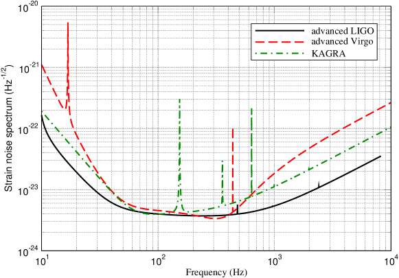
Figure 1: One-sided noise power spectral density for advanced LIGO, advanced Virgo, and KAGRA.

II.2 The Waveform model

The amplitude corrected post-Newtonian (PN) waveforms in the two polarizations (plus and cross), up to the 2.5PN order, were first computed in Ref. Arun et al. (2004) and take the following form,

$$h_{+,\times}=\frac{2M\nu}{D_{L}}x\,\left\{H^{(0)}_{+,\times}+x^{1/2}H^{(1/2)}_{+,\times}+xH^{(1)}_{+,\times}+x^{3/2}H^{(3/2)}_{+,\times}+x^{2}H^{(2)}_{+,\times}+x^{5/2}H^{(5/2)}_{+,\times}\right\}\,.$$ (1)

Here, $M=(m_{1}+m_{2})$ is the total mass of the binary where as $\nu=(m_{1}m_{2}/M^{2})$ is a dimensionless mass parameter which is termed as the symmetric mass ratio and $D_{L}$ denotes the distance to the binary (or luminosity distance). $x$ is the dimensionless PN expansion parameter and is related to the binary’s instantaneous orbital frequency, $F(t)$, as $x=(2\pi MF(t))^{2/3}$ (in units where $G=c=1$). Finally, the coefficients $H^{(n/2)}_{+,\times}$ where $n=0,\cdots,5$, are linear combinations of various harmonics with prefactors that are functions of the inclination angle ($\iota$) of the binary’s angular momentum vector with respect to the line of sight and the symmetric mass ratio $\nu$ (see Arun et al. (2004) for explicit expressions).

The strain in the detector arms due to the signal also depends on the location and orientation of the binary through detector beam pattern functions ( $F_{+}$ and $F_{\times}$) and can be given as

$$h(t)=F_{+}h_{+}(t)+F_{\times}h_{\times}(t)\,,$$ (2)

where $F_{+}$ and $F_{\times}$ in terms of the angular parameters ($\theta,\phi$) giving location of the binary and the polarization angle ($\psi$) giving the binary’s orientation in the plane of sky take the following form

$$F_{+}(\theta,\phi,\psi) = \frac{1}{2}\left(1+\cos^{2}(\theta)\right)\cos(2\phi)\cos(2\psi)-\cos(\theta)\sin(2\phi)\sin(2\psi)\,,$$ (3)

$$F_{\times}(\theta,\phi,\psi) = \frac{1}{2}\left(1+\cos^{2}(\theta)\right)\cos(2\phi)\sin(2\psi)+\cos(\theta)\sin(2\phi)\cos(2\psi)\,.$$ (4)

After combining Eqs. (1)-(4) along with expressions for $H^{(n/2)}_{+,\times}$ listed in Ref. Arun et al. (2004) one can write the expression for the strain in the detector arms as a linear combination of different harmonics of the orbital phase ($\Psi$) in the following way

$$h(t)=\sum_{k=1}^{7}\sum_{n=0}^{5}A_{(k,n/2)}x^{n/2}(t)\cos(k\Psi(t)+\varphi_{(k,n/2)})\,,$$ (5)

where $k$ runs over various harmonics and $n/2$ denotes the PN order. Note that at the 2.5PN order, apart from the dominant harmonic ($k$=$2$), six additional harmonics ($k$=$\{1,3,4,5,6,7\}$) contribute to the waveform. The coefficients $A_{(k,n/2)}$ and the phase offsets $\varphi_{(k,n/2)}$ are functions of the parameters ($D_{L}$, $M$, $\nu$, $\theta$, $\phi$, $\iota$, $\psi$) for the signal observed in the detector and can be assumed to be constants for a given ground-based detector for the duration of the observed signal Van Den Broeck and Sengupta (2007); Van Den Broeck and Sengupta (2007).

Since for the present analysis we shall be using Fisher information matrix approach, it is convenient to use the waveforms in frequency domain. The waveform (2.5PN accurate in amplitude and 3.5PN accurate in phase) in the frequency domain is computed by using the stationary phase approximation, and is given in Ref. Van Den Broeck and Sengupta (2007); Van Den Broeck and Sengupta (2007). We simply recall it here,re

$$\tilde{h}(f) = \frac{2M\nu}{D_{L}}\,\sum_{k=1}^{7}\,\sum_{n=0}^{5}\,\frac{A_{(k,n/2)}\,e^{-\imath\,\varphi_{(k,n/2)}}\,x^{\frac{n}{2}+1}\left(t\left(f_{k}\right)\right)}{2\sqrt{k\dot{F}\left(t\left(f_{k}\right)\right)}}\times e^{\imath(2\pi ft_{c}-\pi/4+k\Psi\left(f_{k}\right))}\,,$$ (6)

where $f_{k}=f/k$ and the Fourier phase $\Psi(f)$ Blanchet et al. (2002) is given by

$$\Psi(f)=-\Phi_{c}+{3\over 256\,\nu}\sum_{j=0}^{7}\psi_{j}\,(2\pi Mf)^{(j-5)/3}\,,$$ (7)

where the coefficients $\psi_{j}$ read

$$\psi_{0} = 1,$$

$$\psi_{1} = 0,$$

$$\psi_{2} = \frac{3715}{756}+\frac{55}{9}\nu,$$

$$\psi_{3} = -16\pi,$$

$$\psi_{4} = \frac{15293365}{508032}+\frac{27145}{504}\nu+\frac{3085}{72}\nu^{2},$$

$$\psi_{5} = \pi\left(\frac{38645}{756}-\frac{65}{9}\nu\right)\left[1+\ln\,\left({f\over F_{LSO}}\right)\right],$$

$$\psi_{6} = \frac{11583231236531}{4694215680}-\frac{640}{3}\pi^{2}-\frac{6848}{21}C+\left(-\frac{15737765635}{3048192}+\frac{2255}{12}\pi^{2}\right)\nu$$

$$+ \frac{76055}{1728}\nu^{2}-\frac{127825}{1296}\nu^{3}-\frac{6848}{63}\ln\left(128\,\pi M\,f\right),$$

$$\psi_{7} = \pi\left(\frac{77096675}{254016}+\frac{378515}{1512}\nu-\frac{74045}{756}\nu^{2}\right).$$ (8)

Here $t_{c}$ and $\Phi_{c}$ appearing in above expressions denote the time and phase at the coalescence epoch. $t_{c}$ can be freely specified in any calculation, and we choose $t_{c}$=$0$. On the other hand, there is a dependence on $\Phi_{c}$ in signal-to-noise ratio and in the Fisher matrix defined in Eq. (26) below. This dependence comes from the cross products of different $k$ modes in $\tilde{h}(f)$. However, such cross product terms are highly oscillating in frequency domain, and their contribution to the integral of Eq. (24) become very small, and the dependence of the final results on $\Phi_{c}$ is not very large. We thus choose $\Phi_{c}=0$ in this paper. To add more to this, we find in our simulations that if we randomly choose our $\Phi_{c}$ in the interval of $[0,2\pi]$, maximum relative change in the error estimation is not more than about $2$-$7$% for any given detector combination or parameter under study. Also note that the quantity $F_{\rm LSO}$ denotes the orbital frequency of the binary at the last stable orbit (LSO) and can be approximated as $F_{\rm LSO}={1/(6^{3/2}\,2\,\pi\,M})$, the orbital frequency at LSO of a test particle moving in Schwarzschild geometry of an object with mass as the total mass ($M$) of the binary in $G=c=1$ units. It turns out that most of the terms (except the ones which are proportional to the factor $\ln f$) appearing in the expression for $\psi_{5}$ given by Eq. (8) can be absorbed into a new definition of $\Phi_{c}$ while performing computations as they have no frequency dependence. Finally, the PN expressions for $\dot{F}$ is given in Van Den Broeck and Sengupta (2007); Van Den Broeck and Sengupta (2007) and we simply recall it here,

$$\dot{F}(f) = \frac{96}{5\pi M^{2}}(2\pi Mf)^{11/3}\left[1-\left(\frac{743}{336}+\frac{11}{4}\nu\right)(2\pi Mf)^{2/3}+4\,\pi(2\pi Mf)\right.$$ (9)

$$\left.\quad+\left(\frac{34103}{18144}+\frac{13661}{2016}\nu+\frac{59}{18}\nu^{2}\right)(2\pi Mf)^{4/3}-\left(\frac{4159\pi}{672}+\frac{189\pi}{8}\nu\right)(2\pi Mf)^{5/3}\right]\,.$$

Before we proceed it is important to note that the term $\dot{F}$ can be treated in many different ways which would lead to small numerical differences in the results. For instance, one can reexpand the factor $1/\sqrt{\dot{F}}$ in the amplitude and then truncate the resulting amplitude at the working PN order Arun et al. (2007, 2007) or one may completely skip performing this reexpansion. In this work we follow the latter treatment and use the expression for $\dot{F}$ at the same PN order as that of the signal amplitude. For instance, when using FWF with 2.5PN amplitude corrections we use the $\dot{F}$ expression which is 2.5PN accurate but we do not perform any reexpansion. We find that the difference to the parameter estimation errors discussed below caused by the difference of this treatment are around at most 7%. Thus, the absolute value of the parameter estimation accuracy might have errors at this level due to this choice. However, the different treatment results in both FWF and RWF in the same way. Thus, the conclusions about the comparison between FWF and RWF do not change.

II.3 Coordinate frames and the detector response

In the previous subsection, we listed expressions for the strain in detector arms (response of the detector to the incoming GW signal) due to the presence of the signal, both in time and frequency domains. It was mentioned there that the response of the detector to the incoming signal also depends on the binary’s position and orientation through beam pattern functions given by Eq. (4). When dealing with a network of detectors which consists of detectors at different locations around the globe, response of each detector to the signal will be different. Reference Pai et al. (2008) shows how a set of rotation transformations between appropriately chosen coordinate systems can tell us the response of each detector. In this section we shall recall the related result of Ref. Pai et al. (2008) for the completeness of the text and refer to the paper for definitions and details. The main idea is as follows.

Let us choose three coordinate frames associated with the wave, detector and the Earth denoted by $\mathbf{x_{w}}\equiv(x_{w},y_{w},z_{w})$, $\mathbf{x_{d}}\equiv(x_{d},y_{d},z_{d})$ and $\mathbf{x_{E}}\equiv(x_{E},y_{E},z_{E})$, respectively (see IIIA of Ref. Pai et al. (2008) for definitions). Let ${\cal O}$ be the rotation operator which transforms one frame to other given three Euler angles. Then if the set ($\phi_{e},\theta_{e},\psi_{e}$) characterizes the transformation between the Earth frame and the wave frame and the set ($\alpha,\beta,\gamma$) characterizes the transformation for the detector-Earth frame, we can have (see Fig. 1 of Ref. Pai et al. (2008) for a graphical display of these transformations)

$$\mathbf{x}_{w} = {\cal O}(\phi_{e},\theta_{e},\psi_{e})\mathbf{x}_{E},$$ (10)

$$\mathbf{x}_{d} = {\cal O}(\alpha,\beta,\gamma)\mathbf{x}_{E}.$$ (11)

In the present convention the source Euler angles ($\phi_{e},\theta_{e},\psi_{e}$) in terms of the angular parameters describing the location ($\theta,\phi$) and the polarization angle ($\psi$) in the Earth frame are given as

$$\phi_{e} =\phi-\pi/2, \theta_{e} =\pi-\theta, \psi_{e} =\psi,$$ (12)

On the other hand, the detector Euler angles $(\alpha,\beta,\gamma)$ are given in terms of the location and orientation of the detector as:

$$\alpha =L+\pi/2,$$ (13)

$$\beta =\pi/2-l,$$ (14)

$$\gamma =\frac{a_{1}+a_{2}}{2}+\frac{3\pi}{2} \text{if $|a_{1}-a_{2}|>\pi$},$$ (15)

$$=\frac{a_{1}+a_{2}}{2}+\frac{\pi}{2} \text{if $|a_{1}-a_{2}|\leq\pi$},$$ (16)

where $l$ and $L$ are the latitude and longitude of the detector site. The angles $a_{1}$ and $a_{2}$ describe the orientation of the first and second arm, respectively. In Table 1 of this paper we provide the information about the location and orientation of various detectors considered in this analysis.

Table 1: Location and orientation information of the future Earth-based interferometric GW detectors LIG ; Pai et al. (2001). The location of each detector is given in terms of the latitude and longitude. The orientation of an arm is given by the angle through which one must rotate it clockwise (while viewing from top) to point the local North. The corresponding detector Euler angles $(\alpha,\beta,\gamma)$ are listed. Note that, for the location of the LIGO-India detector we use the values listed in Table I of Ref. Schutz (2011). This location was chosen as a fiducial site for the detector.

Detector	Vertex	Vertex	Arm 1	Arm 2	$\alpha$	$\beta$	$\gamma$
	latitude (N)	longitude (E)	$a_{1}$	$a_{2}$
LIGO Livingston (L)	$30^{\circ}33^{\prime}46.4196^{\prime\prime}$	$-90^{\circ}46^{\prime}27.2654^{\prime\prime}$	$107.72^{\circ}$	$197.72^{\circ}$	$-0.77^{\circ}$	$59.44^{\circ}$	$242.72^{\circ}$
LIGO Hanford (H)	$46^{\circ}27^{\prime}18.528^{\prime\prime}$	$-119^{\circ}25^{\prime}27.5657^{\prime\prime}$	$36^{\circ}$	$126^{\circ}$	$-29.41^{\circ}$	$43.55^{\circ}$	$171.0^{\circ}$
VIRGO (V)	$43^{\circ}37^{\prime}53.0921^{\prime\prime}$	$10^{\circ}30^{\prime}16.1878^{\prime\prime}$	$340.57^{\circ}$	$70.57^{\circ}$	$100.5^{\circ}$	$46.37^{\circ}$	$116.0^{\circ}$
KAGRA (K)	$36^{\circ}14^{\prime}60^{\prime\prime}$	$137^{\circ}10^{\prime}48^{\prime\prime}$	$295^{\circ}$	$25^{\circ}$	$227.18^{\circ}$	$53.75^{\circ}$	$70^{\circ}$
LIGO-India (I)	$19^{\circ}05^{\prime}47^{\prime\prime}$	$74^{\circ}2^{\prime}59^{\prime\prime}$	$45^{\circ}$	$135^{\circ}$	$164.05^{\circ}$	$70.90^{\circ}$	$180^{\circ}$

The coordinate transformation between the wave frame and the detector frame can be obtained by combining Eq. (10) and Eq. (11)

$$\mathbf{x}_{w}={\cal O}(\phi^{\prime}_{e},\theta^{\prime}_{e},\psi^{\prime}_{e})\mathbf{x}_{d}\,,$$ (17)

where ${\cal O}(\phi^{\prime}_{e},\theta^{\prime}_{e},\psi^{\prime}_{e})\equiv{\cal O}(\phi_{e},\theta_{e},\psi_{e}){\cal O}^{-1}(\alpha,\beta,\gamma)$.

It should be evident from the above that, transformations associating the detector frame with the wave frame can be split into two rotations: one from the detector frame to the Earth frame and one from the Earth frame to the wave frame. These two successive transformations can be translated into the addition theorem of Gel’fand functions Gel’fand and Shapiro (1963), which reads as

$$T_{mn}(\phi^{\prime}_{e},\theta^{\prime}_{e},\psi^{\prime}_{e})=\sum_{l=-2}^{2}T_{ml}(\phi_{e},\theta_{e},\psi_{e})T^{*}_{nl}(\alpha,\beta,\gamma)\,,$$ (18)

where $T_{ij}$ denotes the Gel’fand functions. The detector response due to the incoming GW (or the strain induced by the signal in the detector arms) is given by Eq. (2) which in a more compact notation can be written as

$$h(t)\equiv\Re[f_{c}^{*}\,h_{c}]\,,$$ (19)

where $f_{c}=F_{+}+i\,F_{\times}$ and $h_{c}=h_{+}+i\,h_{\times}$ are defined as complex antenna pattern function and complex GW signal, respectively (see the discussion in Sec. IIB and in Appendix A of Ref. Pai et al. (2008)), where the (*) indicates the complex conjugate of $f_{c}$, and $\Re$ represents the real part.

In addition to this, since detectors in the network will be located at different places around the globe, the incoming GW signal shall arrive at various detector sites at different instances. In order to correctly account for the time delays between the arrival times at different detectors one has to choose a reference frame with respect to which all the time measurements are performed. Following Ref. Pai et al. (2008) we choose this reference frame to be the frame attached to the center of the earth. In such case the response of $I$-th detector (after folding in the effect of delays)

$$h^{I}(t)\equiv\Re[f_{c}^{I*}h_{c}(t-\tau_{I}(\theta,\phi))]\,,$$ (20)

where $\tau_{I}(\theta,\phi)=({\bf r_{I}}-{\bf r_{E}})\cdot{\bf w}(\theta,\phi)/c$, denotes the time-delay in the arrival times of the incoming signal at the detector and at the center of the Earth. Quantities ${\bf r_{I}}$ and ${\bf r_{E}}$ denote the vectors directed to locations at the detector and the Earth’s center, from the origin of the reference frame chosen (here it is Earth’s center itself). ${\bf w}(\theta,\phi)$ is the unit vector along the propagation of the wave with $\theta$, $\phi$ again giving the source location in a frame attached to the center of the Earth and $c$ denotes the speed of light.

It was discussed in detail in the appendix of Ref. Pai et al. (2008) that one can write the complex pattern function ($f_{c}$ above) in terms of Gel’fand functions as (see Eq. (B13) there)

$$f_{c}^{I}=\sum_{s=-2}^{2}iT_{2s}(\phi_{e},\theta_{e},\psi_{e})[T_{2s}(\alpha,\beta,\gamma)-T_{-2s}(\alpha,\beta,\gamma)]^{*}.$$ (21)

Given the source Euler angles ($\phi_{e},\theta_{e},\psi_{e}$) and the $I$-th detector Euler angles ($\alpha^{I},\beta^{I},\gamma^{I}$) given by Eq. (12) and Eq. (16), along with definition of Gel’fand functions, one can calculate $f_{c}^{I}$ for a given $I$-th detector and hence the response of individual detectors to the signal both in time and frequency domain. With these inputs we go on to describe our parameter estimation strategy in the next section.

II.4 Error Estimation

The inspiral signal from the nonspinning compact binary systems can be characterized in terms of total nine parameters (see Sec. II.2 above). This means we have a nine dimensional parameter space which reads

$$\mathbf{p}=\{\ln D_{L}\,,{\cal M}_{c},\delta,t_{c},\Phi_{c},\cos(\theta),\phi,\psi,\cos(\iota)\}\ \,,$$ (22)

where, ${\cal M}_{c}=M\,\nu^{3/5}$ is termed as the Chirp Mass and $\delta=|m1-m2|/m$ is called the difference mass ratio parameter. We employ the Fisher matrix approach Finn (1992); Finn and Chernoff (1993) to see how well we can constrain these parameters. Below we briefly discuss our strategy for estimating various parameters of the source which is based on the Fisher matrix approach. We first define the matched filter signal-to-noise ratio (SNR) of a network of $N$ detectors, $\rho$, as

$$\rho = \left[\sum_{I=1}^{N}(h^{I}|h^{I})_{I}\right]^{1/2}.$$ (23)

Here, $(\,|\,)_{I}$ denotes the noise weighted inner product for $I$-th detector. In general, for any two functions $g$ and $h$, their inner product is defined as:

$$(g\,|\,h)_{I}\equiv 4\Re\int_{f_{min}}^{f_{max}}df\,\frac{\tilde{g}^{*}(f)\,\tilde{h}(f)}{S_{h}^{(I)}(f)}.$$ (24)

Here $S_{h}^{(I)}(f)$ represent the one-sided noise power spectral density of $I$th detector. The limits of integration $[f_{min},f_{max}]$ are determined by both the detector and by the nature of the signal. Since we are using inspiral waveform, which is usually not reliable beyond the last stable orbit we can choose to terminate the integrals when the last stable orbit is reached. For instance, we assume that the contribution from $k$th harmonic to the waveform is zero above the frequency $kF_{\rm LSO}$, where $F_{\rm LSO}$ is the orbital frequency at the last stable orbit Van Den Broeck and Sengupta (2007). Since the amplitude-corrected waveform we are using in this work has seven harmonics, we set the upper cutoff to be 7$F_{\rm LSO}$ when we use the FWF in the analysis. For lower cutoff, as power spectral densities $S_{h}(f)$ tend to rise very quickly below a certain frequency $f_{s}$ where they can be considered infinite for all practical purposes, we may set it to be $f_{s}$.

Let $\tilde{\theta}_{a}$ denote the ‘true values’ of the parameters and let $\tilde{\theta}_{a}+\Delta\theta_{a}$ be the best-fit parameters in the presence of some realization of the noise. Then for large SNR, error in the estimation of parameters $\Delta\theta_{a}$ obey a Gaussian probability distribution Helström (1968); Wainstein and Zubakov (1962); Finn (1992); Finn and Chernoff (1993) of the form

$$p({\bf\Delta\theta})=p^{(0)}\exp\left[-\frac{1}{2}\Gamma_{bc}\Delta\theta_{b}\Delta\theta_{c}\right],$$ (25)

where ${{\bf\Delta\theta}=\{\Delta\theta_{a}\}}$ and repeated indices are summed up. The $p^{(0)}$ is a normalization constant. The quantity $\Gamma_{ab}$ appearing in Eq. (25) is the Fisher information matrix and is given by,

$$\Gamma_{ab}=(h_{a}\,|\,h_{b})$$ (26)

where $h_{a}\equiv\partial h/\partial\theta^{a}$. Using the definition of the inner product, one can reexpress the Fisher matrix associated with the $I$-th detector $\Gamma_{ab}^{I}$ more explicitly as

$$\Gamma_{ab}^{I}=(h_{a}^{I}\,|\,h_{b}^{I})_{I}\equiv 4\int_{f_{s}}^{k\,F_{LSO}}df\,\frac{\Re([\tilde{h}_{a}^{I}(f)]^{*}[\tilde{h}_{b}^{I}(f)])}{S_{h}(f)}\,,$$ (27)

The Fisher matrix for a network of $N$ detectors is simply the sum of individual Fisher matrices associated with different detectors and is given by

$$\Gamma_{ab}=\sum_{I=1}^{N}\Gamma_{ab}^{I}$$ (28)

The covariance matrix, defined as the inverse of the Fisher matrix, is given by

$$\Sigma_{ab}\equiv\langle\Delta\theta_{a}\Delta\theta_{b}\rangle=({\Gamma_{ab}})^{-1},$$ (29)

where $\langle\cdot\rangle$ denotes an average over the probability distribution function in Eq. (25). The root-mean-square error $\sigma_{a}$ in the estimation of the parameters $\theta_{a}$ is

$$\sigma_{a}=\bigl{\langle}(\Delta\theta_{a})^{2}\bigr{\rangle}^{1/2}=\sqrt{\Sigma_{aa}}\,,$$ (30)

II.5 Numerical simulations

As discussed in Sec. I, in this paper we investigate the parameter estimation problem for a compact binary system consisting a NS ($1.4M_{\odot}$) and a BH ($10M_{\odot}$). Despite the fact that BNS systems are expected to be seen more often in ground-based detectors as compared to the NS-BH systems, here we chose to study asymmetric systems. This is because the contribution from odd harmonics (k=1,3,5,7) is directly proportional to the asymmetry of the system described by the parameter $\delta=|m_{1}-m_{2}|/M^{2}$. This would mean that for symmetric or nearly symmetric systems (such as BNS systems) such terms either would not contribute or shall have small effects. Since one of the prime goals of the present study is to investigate the improvements in parameter estimation accuracies due to inclusion of subdominant modes of the signal we must choose a system which is sufficiently asymmetric. Hence, we expect that with increasing asymmetry of the binary, subdominant modes of the signal become more and more important (as also odd ones would then start contributing significantly) which eventually leads to better estimation of parameters. Moreover, effects of subdominant harmonics are expected to be more important for heavier systems as the dominant mode fails to enter the sensitive part of detector bandwidth Van Den Broeck and Sengupta (2007); Arun et al. (2007). However, it should be noted that parameter estimation shall in general be poor for such systems as they will be observed with smaller SNRs (since the dominant harmonic either does not contribute or its contribution is negligible). Another reason is related to the question of correctness of the PN waveform itself for systems heavier than 12$M_{\odot}$ and with larger mass ratios (as different approximants start showing deviations from each other) Buonanno et al. (2009). We could have considered even more asymmetric NS-BH systems, for which the effect of subdominant modes would be even more. But one should bear in mind that, for heavier NS-BH binaries, the neglect of merger and ringdown waveforms are going to be even more important than PN subdominant modes and hence we do not consider them here. Keeping the above constraints in mind we choose to study a population of NS-BH system with neutron star mass as $1.4M_{\odot}$ and BH mass as $10M_{\odot}$.

We assume a population of NS-BH systems ((1.4-10)$M_{\odot}$), all placed at a luminosity distance of 200 Mpc. The choice of the distance is rather arbitrary. The results of the parameter estimation error for 9 parameters are inversely proportional to the distance for both FWF and RWF, and for any detector combinations. Let the parameter estimation errors (30) with distance $r$ to be $\sigma_{a}^{r}$. The parameter estimation errors with other distance $r=r^{\prime}$ is given as $\sigma_{a}^{\rm 200Mpc}r^{\prime}/(200$Mpc).

In total we consider 12800 realizations of the source uniformly distributed over the sky and obtained by randomizing the angular parameters specifying the location ($\cos(\theta),\phi$) and orientation ($\cos(\iota),\psi$) of the binary. The nine-dimensional parameter space given by Eq. (22) shall lead to the $9\times 9$ Fisher matrix which is further used to compute errors in various parameters for each one of these realizations. However, errors in $\cos(\theta)$ and $\phi$ can be combined to give error in the solid angle ($\Omega$) centred around the source. Following Barack and Cutler (2004), we define

$$\Delta\Omega_{S}=2\pi\sqrt{\sigma^{2}_{\cos(\theta)}\sigma^{2}_{\phi}-\Sigma^{2}_{\cos(\theta)\,\phi}}$$ (31)

where $\Sigma_{\cos(\theta)\,\phi}$ is the covariance between $\cos(\theta)$ and $\phi$.

As discussed in Barack and Cutler (2004), the probability that the source lies outside an error ellipse enclosing solid angle $\Delta\Omega$ is $e^{-\Delta\Omega/\Delta\Omega_{S}}$. We then adopt $\Delta\Omega_{95}\equiv 3\Delta\Omega_{S}$ as our definition of the source localization error, which represents approximately 95% confidence region of the localization error ellipses.

II.6 Accuracy of the numerical computation

The covariant matrix is obtained by inverting the Fisher matrix. In this paper, this is done numerically with the LU decomposition in the GSL library GSL . Some of the results are also computed and are confirmed with MATHEMATICA MAT . Numerical inversion of matrices often suffer from the problem of accuracy due to the ill-conditioned Fisher matrices. We check the accuracy of the matrix inversion by multiplying the inverse with the original matrix, and check the deviation of it from the identity matrix. Similar to Berti et al. Berti et al. (2005), we define $\epsilon_{\rm inv}=\max_{i\neq j}|\left(\Gamma\,\Sigma\right)_{ij}|$, and use it as a measure of the accuracy of the matrix inversion.

We find that in the case of FWF, $\epsilon_{\rm inv}$ is distributed in a Gaussian-like form with mean value of around $10^{-12}$, and the maximum is about $10^{-10}$. Since the numerical computation is done with double precision, the round off error is around $10^{-15}$, we can say that this accuracy is good enough. On the other hand, in the case of RWF, the distribution of $\epsilon_{\rm inv}$ has a tail at larger value up to $\sim 10^{-3}$. In addition, we also find the correlation between ($\sigma_{\ln D_{L}}$, $\sigma_{\Phi_{c}}$, $\sigma_{\psi}$, $\sigma_{\cos\iota}$) and $\epsilon_{\rm inv}$.

The error of the matrix inversion for RWF is caused by the ill condition of the Fisher matrix. It mainly occurs when $\iota$ is near $0$ or $\pi$. In such cases, the derivatives of $\tilde{h}(f)$ with respect to $\ln D_{L}$ and $\cos(\iota)$ become nearly proportional to each other, which makes the Fisher matrix ill conditioned. On the other hand, because of the complex dependence of the amplitude of FWF on $\cos(\iota)$, such a problem does not occur in the case of FWF.

Since we can not trust the results of the cases with large $\epsilon_{\rm inv}$, we decided not to use the results with $\epsilon_{\rm inv}>10^{-8}$. With this prescription, around 5% of the cases for RWF are removed and are not used in the final results. We checked that if we change the criteria to $\epsilon_{\rm inv}>10^{-10}$, the median of $\sigma_{\ln D_{L}}$, $\sigma_{\psi}$, and $\sigma_{\cos\iota}$ are changed at most about 30%. The changes of the median error of $\sigma_{\Phi_{c}}$ is at most 13%. The changes of the median error of $\Delta\Omega$ is at most 16%. The changes of the median errors of other parameters are at most 10%. We conservatively adopt these value as estimate of the accuracy of the median of the error of the parameter estimation.

In addition to the accuracy of the matrix inversion, in the Fisher matrix analysis, there is a problem in low SNR cases. We find that, for a small fraction of the source population, the network SNR is smaller than the value 8. Since, the Fisher matrix approach can not be trusted for weak signals (those with smaller SNRs), we remove such cases from our final results. As a result, about $5$ % of cases for both FWF and RWF are removed for the 3 detector cases. Note however that this does not change the median of the error of all parameters significantly. The change is only about $8$% for all parameters. When the number of detector is 4 or 5, the network SNR is larger than 3 detector cases. Thus, the effect of this SNR threshold is smaller than these value.

III Results

The results of our exhaustive parameter estimation exercise and interpretations of the trends observed are discussed in this section. The improvement in the parameter estimation due to the use of FWF in the multidetector framework comes from a combination of two independent contributions: the improvement due to additional features of FWF and the effect of additional detectors which observe the signal. Hence the first part (III.1) of the section discusses the effect of FWF on parameter estimation as compared to the RWF and in the second part (III.2) we compare our results for various detector combinations with three or more detectors. We choose to quantify the measurement accuracy of various parameters by the median values of the error distributions since the median is unaffected by the tail of the distribution. Further, the width of the distribution is given by the inter-quartile range. The inter-quartile range (denoted by Q3-Q1) is defined as the difference between the third (Q3: upper quartile) and the first quartile (Q1: lower quartile) and represents the width of the distribution around the median. Thus the two numbers collectively give the range in which error in the measurement of a parameter varies about the median error for 50% of the population.

III.1 Effect of the use of FWF over RWF on parameter accuracy

III.1.1 LHV

In this section we aim to study the effects of using the FWF over the RWF on measurement accuracies of various parameters in context of the LIGO-Virgo (LHV) network. Note that here we choose to display the error distributions for only four of the nine parameters ($D_{L}$, $\cos(\iota)$, $\Phi_{c}$, and $\psi$) (see Fig. 2). This is mainly to avoid proliferation of graphical details, as in the case of other parameters the error distributions corresponding to the two cases (RWF and FWF) largely are same both in shape and in positioning. However, we display medians of error distributions corresponding to all nine parameters in Table 2. Different panels in Fig. 1 also display two numbers corresponding to the median and the interquartile range.

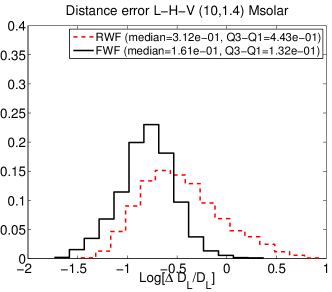
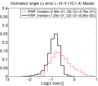
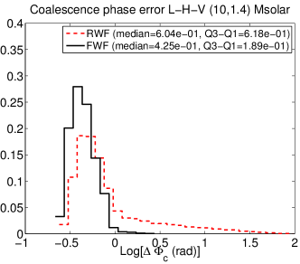
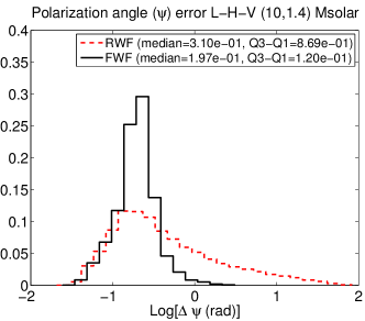
Figure 2: Figure displays error distributions corresponding to the luminosity distance ($D_{L}$), cosine of the inclination angle ($\cos(\iota)$), phase at the time of coalescence ($\Phi_{c}$) and the polarization angle ($\psi$), in context of the LIGO-Virgo network (LHV). The study has been performed for a population of ($1.4-10$)$M_{\odot}$ NS-BH binaries, all placed at 200 Mpc and distributed and oriented uniformly over the sky surface. The error distributions obtained by choosing two different waveform models for signals from the source, the restricted waveform (RWF) and the full waveform (FWF), are compared. Since the error distributions are asymmetric (usually with a long tail) we chose ”median” as a reliable measure of accuracies with which parameters are measured. In addition we also wish to give the interquartile range, represented by Q3-Q1 [ difference between the upper quartile (Q3) and the lower quartile (Q1) ], corresponding to each error distribution. Median and the interquartile range (Q3-Q1) corresponding to each parameter has been displayed in various panels. Note that out of nine parameters listed in Eq. (22) we are displaying graphical results only for four of them since effect of the use of FWF over RWF is only significant in these four cases. However, in Table 2 we list medians corresponding to error distribution of all the parameters.

It should be obvious from the shifts observed in different panels of Fig. 2 that the FWF indeed significantly improves the measurements of the parameters ($D_{L}$, $\cos(\iota)$, $\Phi_{c}$, and $\psi$). This is not surprising as in general the FWF, by the virtue of contributions from subdominant modes, has a great deal of structure, which enables one to extract parameters of the source more efficiently as compared to the case when RWF is used (see Ref. Van Den Broeck and Sengupta (2007) for a discussion). Comparing the median of distributions related to the errors in $D_{L}$ and $\cos(\iota)$ we find that the accuracies with which the two parameters will be measured will improve by almost a factor of about 2 and those related to $\Phi_{c}$ and $\psi$ improve by a factor of about 1.5. It is noteworthy that we find such improvements despite slightly smaller signal-to-noise ratio (SNR) for the FWF cases.

To quantify this we rescale errors to values that correspond to a SNR of 20. Median errors for the fixed SNR case has been given in Table 3. After comparing RWF and FWF errors for $D_{L}$, and $\cos(\iota)$ we find that improvement factors are still about 2. The main reason for such improvements in measurement of $D_{L}$ and $\cos(\iota)$, when FWF is used, is the fact that, in the RWF case, there persists a degeneracy between the two parameters which breaks when one uses the FWF. To elaborate more, the FWF in contrast to the RWF contains additional information about the inclination angle of the binary through amplitude corrections, which enables one to measure the inclination angle parameter with much better accuracy. Further, since inclination angle and the distance to the binary are strongly correlated with each other, accuracy of distance measurement also improves. It was argued in Ref. Arun et al. (2005) that the trends in the measurement of parameters which are strongly correlated can be understood in terms of the related correlation coefficients. It was argued there that a decrease (increase) in correlation coefficients indicates better (worse) measurement of related parameters. As an example, we compare the median of the correlation coefficient (absolute value) in context of LHV network which are shown in the top in Tables 4 and 5. The correlation coefficient between $D_{L}$ and $\cos(\iota)$ is 0.95 for the RWF case. We find that this value decreases slightly to a value of 0.91 for the FWF case. We have checked that, by considering the accuracy of inversion of Fisher matrices and the number of simulation of order $10^{4}$, the numerical and the statistical errors are much less than this difference, and this difference is significant. Although the difference is small, this is effective to reduce the error of $D_{L}$ and $\cos(\iota)$ for the FWF case. We show examples of the 2 dimensional contour of the error in the $D_{L}-\cos(\iota)$ plane for the LHV case in Fig.  3. We can see that the reduction of the correlation coefficient helps the improvement of the distance and the inclination angle measurement. We also find that when $\iota\lesssim 0.8$, the difference between FWF cases and RWF cases become very large. One the other hand, when $\iota\gtrsim 0.9$, the difference between FWF and RWF is small. This is because when $\iota$ is closer to $\pi/2$, $\cos(\iota)$ becomes smaller and the difference between FWF and RWF become smaller.

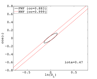
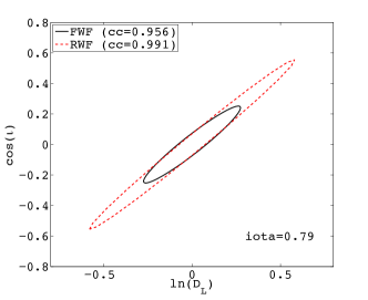
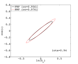
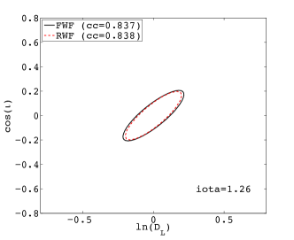
Figure 3: Figure displays two-dimensional contour of the error of $D_{L}$ and $\cos(\iota)$ for four different values of $\iota$ in the LHV case. The other angle parameters are $\theta=\pi/3$, $\phi=\pi/3$, and $\psi=\pi/4$. $cc$ denotes the value of the correlation coefficient between $D_{L}$ and $\cos(\iota)$ computed from the covariant matrix $\Sigma_{ab}$. The contour corresponds to the 68% error region.

At this stage we would like to point out that GWs from binary systems with at least one component as NS, will be observed with some electromagnetic counterpart (as a recent reference, see Singer et al. (2014)). In such a situation, electromagnetic (EM) observations can be used to fix the location as well as the distance to the binary (using redshift measurements), which completely breaks the $D_{L}$-$\iota$ degeneracy and hence further significantly improves the $\iota$ measurements. An analysis under the assumption of coincidence GW-EM observations has been performed in the case of binary NS (BNS) and BH-NS systems (which are strong candidates for progenitors of short-hard gamma ray bursts (SGRBs)) in Ref. Arun et al. (2014). It has been shown there that once the information about the source location and its distance is folded in the analysis, one can put tight constraints on the inclination angle measurements, which further can help us understand various aspects of SGRB science.

Improvement in the measurement of the coalescence phase ($\Phi_{c}$) can be understood as an effect of the fact that the FWF has more information about this parameter as compared to that present in the RWF as different harmonics enter the sensitivity band of the detector at different times. Next, we find that the $\Phi_{c}$-$\psi$ component of the correlation coefficient matrix, reduces to a value of 0.43 for FWF from its RWF value of 0.58. This explains why we see an improvement in the measurement of $\psi$ when the FWF is used over the RWF.

As far as other parameters are concerned we do not see much improvement due to the use of the FWF over the RWF (see Table 2). For instance, the mass parameters can be very well measured using the phase information which is already present in the RWF and hence additional information about the mass parameters present in the amplitude leads to minor improvements in the measurement accuracies of mass parameters. On the other hand, measurement of $t_{c}$, $\theta$ and $\phi$ basically depend on the time-delays between different detector sites which for a given network are same irrespective of the waveform model involved. However, since the polarization angle is better measured when FWF is used, improvements in the measurement of location angular parameters ($\theta$, $\phi$) are expected, since they enter the waveform in more or less similar ways through the antenna pattern functions (see Eq. (4)), and hence they are expected to be strongly correlated (see also the related discussion in Van Den Broeck and Sengupta (2007)). Upon comparing correlation coefficients related to $\theta$-$\phi$-$\psi$ pairs we find that for the FWF case correlations are significantly small as compared to the RWF case. However, one should also keep in mind that the correlations between these parameters are not so strong for the network case. This is expected as in the case of a network various degeneracy among angular parameters break which makes various quantities relatively independent of each other. This would mean that although when going from RWF to FWF correlations are significantly reduced, the measurements of one parameter would affect weakly the measurement of the other. This is why we only see small a improvement in $\theta$ and $\phi$ which further leads to small improvements in angular resolution. In addition, we notice that $t_{c}$ has moderately strong correlations with ${\cal M}_{c}$, $\delta$, $\Phi_{c}$, $\theta$ and $\phi$. We find that when going from RWF to FWF, for some pairs correlations decrease (which would lead to better in parameter estimation (PE)) and for the rest it increases (worsening the PE). It is the combined effect of various correlations that we see an effective minor improvement in $t_{c}$.

III.1.2 LHVK

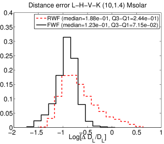
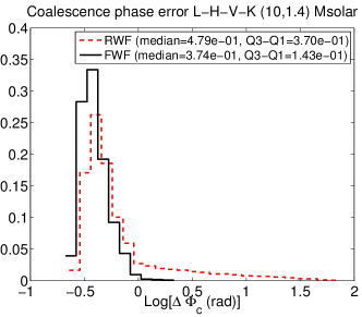
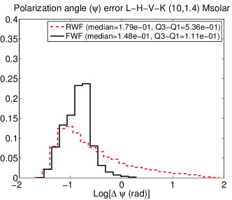
Figure 4: Figure displays error distributions corresponding to the ($D_{L},\cos(\iota),\Phi_{c},\psi$), in context of the LIGO-Virgo-KAGRA network (LHVK). The study has been performed for a population of (1.4-10)$M_{\odot}$ NS-BH binaries, all placed at 200 Mpc and distributed and oriented uniformly over the whole sky. The error distributions for signals with RWF and FWF, are compared. Median and the inter-quartile range (Q3-Q1) corresponding to each parameter has been displayed in various panels. Note that out of nine parameters listed in Eq. (22) we are displaying graphical results only for four of them since effect of the use of FWF over RWF is only significant in these four cases. However, in Table 2 we list medians corresponding to error distribution of all the parameters.

In the previous subsection we discussed the accuracies with which various parameters are measured in the context of the LIGO-Virgo network (LHV). We also tried to understand possible reasons for the improvements in estimating various parameters when FWF is used as compared to the RWF in LHV network. The LHV network is expected to be operational by early 2016. However, as discussed in Sec. II.1, the Japanese detector KAGRA is expected to be fully operational by the end of year 2018, and hence by that time we might have a 4-detector network, LIGO-Virgo-KAGRA (LHVK). The addition of the fourth detector would not only increase the duty cycle of the detector networks but also would improve the localization of the source (see below and the discussion in Sec. III.2). Error distributions corresponding to parameters $D_{L}$, $\cos(\iota)$, $\Phi_{c}$ and $\psi$, in the context of the LIGO-Virgo-KAGRA (LHVK) network, has been displayed in Fig. 4.

Median errors displayed in each panel of Fig. 4 suggest that the use of FWF over RWF shall improve the measurements of $D_{L}$, and $\cos(\iota)$ by a factor of about 1.5 and those of $\Phi_{c}$ and $\psi$ by factors of 1.3 and 1.2, respectively. As far as the measurement of other parameters are concerned, the improvement is still very small and we do not wish to show graphical results corresponding to these parameters for the reason mention in the previous subsection. However, we list median errors in Table 2. Note that here also we can find that the effects of the SNR is only minor in error estimation as was seen in the LHV case (see Table 2- 3). The reason behind the improvements in various parameters is again similar to those discussed in the previous section. However, note that as compared to LHV case the measurement accuracies with LHVK case are much better. As we shall discuss in detail in the Sec. III.2, this is due to the fact that the coherent SNR for LHVK is larger than the LHV case. In particular, angular resolution improves significantly with the inclusion of the fourth detector in the network as LHVK would have larger effective area as compared to the one LHV case, which in turn guarantees better localization. We postpone the discussion related to the angular resolution to Sec. III.2.

III.1.3 LHVKI

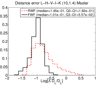
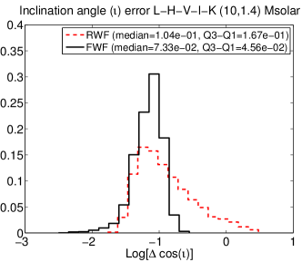
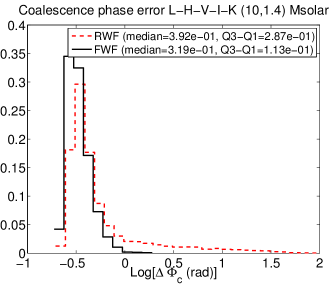
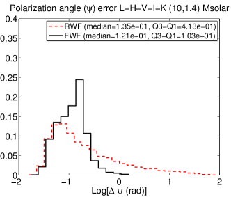
Figure 5: Figure displays error distributions corresponding to the ($D_{L},\cos(\iota),\Phi_{c},\psi$), in context of the LIGO-Virgo-LIGO-India-KAGRA network (LHVKI). The study has been performed for a population of (1.4-10)$M_{\odot}$ NS-BH binaries, all placed at 200 Mpc and distributed uniformly over the sky surface. The error distributions for signals with RWF and FWF, are compared. Median and the inter-quartile range (Q3-Q1) corresponding to each parameter has been displayed in various panels. Note that out of nine parameters listed in Eq. (22) we are displaying graphical results only for four of them since effect of the use of FWF over RWF is only significant in these four cases. However, in Table 2 we list medians corresponding to error distribution of all the parameters.

Just as adding the Japanese detector KAGRA to the LIGO-Virgo (LHV) network improves measurements of various parameters as well increases the duty cycle of the detector networks, addition of LIGO-India will guarantee better measurement of various parameters as compared to the three and four detector networks. Similar to Figs. 2-4 the error distributions for $D_{L}$, $\cos(\iota)$, $\Phi_{c}$ and $\psi$ is displayed in Fig. 5 in context of the 5-detector network LHVKI. For this case median errors in $D_{L}$, and $\cos(\iota)$ improve by a factor of about 1.4 and those for $\Phi_{c}$ and $\psi$ by factors of about 1.2 and 1.1, respectively. The measurements of all other parameters improve by even smaller factors when FWF is used as compared to the RWF. Note that although the median errors suggest that using RWF one can measure parameters with almost similar accuracies as with FWF, for a number of cases RWF still gives very large errors. This suggests that using FWF would make sure that systematic effects do not bias the measurements. In the next section we shall compare the benefits of having a network with large number of detectors in context of parameter estimation by taking examples of the three different combinations (LHV, LHVK, and LHVKI).

When looking at localization error for various detector combinations in Table 2 we notice that for all 3-detector cases the localization is better when FWF is used, whereas for all 4-detector and the 5-detector cases, the use of RWF leads to better localization. However, when we look at the localization errors for fixed SNR cases (Table 3), we do not see these two opposite trends; for all detector combination the use of FWF gives better localization. Let us try understanding first the two opposite trends we see in Table 2. We notice, for all 3-detector cases, FWF works better (in localizing the source), despite the fact that the FWF SNR is smaller than RWF SNR. This can be understood by recalling the arguments presented in Sec. III.1.1, in context of better measurement of location angle parameters ($\theta$, $\phi$) with FWF, which further leads to better localization. Trends in Table 2 suggest that for all the 3-detector cases, whatever degradation happens because of smaller SNR in FWF cases is in fact compensated by the better measurement of location angle parameter. Also it is noteworthy that the difference between the RWF and FWF SNR is very small, hence more or less SNR does not play a significant role in the case of 3-detector networks. However, when we add fourth and fifth detector to the network, coherent SNR for RWF cases become significantly larger than the coherent SNR for FWF cases. However, as was argued in Sec. III.1.1, as more detectors are included in the network, various degeneracy between the angular parameters are resolved and hence measurements of different angular parameters becomes almost independent of each other even in the case of RWF, and hence milds down the effect of FWF which played an important role in three detector cases. These two arguments combined explain why we see two opposite trends in the Table 2. However, when we look at the fixed-SNR table (Table 3), the SNR does not play a role and in that case the FWF of course would perform better, and this is why the use of FWF gives better localization for all detector combinations as can be seen in Table 3. Note that the addition of fourth and fifth detector to the network will anyway improve the localization irrespective of the waveform used.

III.2 Comparison of effects of various multidetector networks on parameter accuracies

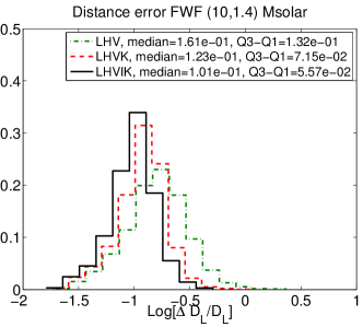
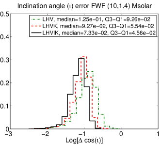
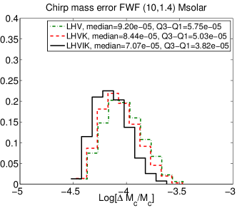
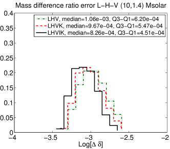
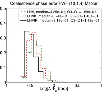
Figure 6: Comparisons of error distributions of various parameters ($D_{L}$, $\cos(\iota)$, $M_{c}$, $\delta$, $\Phi_{c}$ and $\psi$) with three different networks (LHV, LHVK, and LHVKI) has been displayed. The study has been performed for a population of (1.4-10)$M_{\odot}$ NS-BH binaries, all placed at 200 Mpc and distributed uniformly over the sky surface. Error distributions displayed here have been obtained using the amplitude corrected approximate inspiral waveform of the GW signal expected from the source. Various panels also display median and the inter-quartile range for each error distribution.

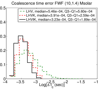
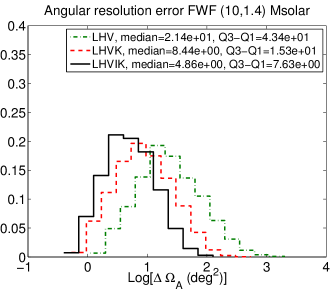
Figure 7: Same as Fig. 6 but error distributions correspond to the coalescence time $t_{c}$ and solid angle around source’s location $\Omega$.

In previous subsections we discussed how the use of the FWF over the RWF improves measurements of various parameters in context of three representative network combinations which were chosen to be LHV, LHVK, and LHVKI. This choice was mainly based on a time-line argument that when detectors would start operating. However, we find that LHV, LHVK and LHVKI can also be assumed to be representative configurations within the respective class of network configurations as the error estimation within a class does not vary significantly. Hence, in this section we aim to make rigorous comparisons of our PE results in context of our three representative detector configurations LHV, LHVK, and LHVKI. We shall refer to Table 2 for the median errors in various parameters in context of all possible network configurations.

The parameter estimation accuracies for our three representative network combinations are displayed in Figs. 6-7. Figure 6 displays error distributions for $D_{L}$, $\cos(\iota)$, ${\cal M}_{c}$, $\delta$, $\Phi_{c}$ and $\psi$. On the other hand, Fig. 7 displays the error distributions for $t_{c}$ and the angular resolution $\Delta\Omega$. Note that here we chose to display the error distribution for the angular resolution and not the ones related to the angular parameters giving the location of the source ($\theta$, $\phi$). This is so because the errors in $\theta$ and $\phi$ and the covariances between them can be suitably combined to obtain the solid angle around the location of the source (see Eq. (31)) which precisely tells how well the source can be localized by the given network (the angular resolution of the network). Also note that while comparing different network we only use PE results obtained using the FWF which is a better approximation to the actual signal. Even a quick look at the shapes and respective positioning of error distributions corresponding to various parameters appearing in Figs. 6-7 reveal that measurement accuracies improve by the addition of the fourth and the fifth detector to the three detector network. This is true in general for all the detector combinations (see Table 2). This is indeed what is expected in general as the coherent SNR is larger for a network which consists of more detectors which in turn improves the estimation of parameters. However, it is not the end of the story. The unobvious is revealed when we look at the fixed SNR case results listed in Table 3. Comparing the FWF median errors corresponding to our three representative cases we find that the improvement is not entirely due to the larger SNR for detector networks with larger number of detectors but some other effects are also play significant roles. Below we try to quantify these effects in the light of results displayed in Table 3.

• Localization: Upon comparing median errors corresponding to the FWF cases in context of our representative network combinations listed in Table 3 we find that angular resolution improves by a factor of about 2.2 and 3.4 as one adds KAGRA and both KAGRA and LIGO-India to the LHV network, respectively. This can be understood in the following way.

  Since both LHVK and LHVKI networks shall involve pairs of detectors with baselines larger than the ones in the LHV network, an improvement in the angular resolution is indeed expected as the angular resolution goes roughly as the square of the distance between the two detectors. More precisely it is the area of the triangle formed by three detectors in the network which decides which 3-detector network shall give the best angular resolution Pai et al. (2001). For instance, we find that among the 3-detector networks LVK has the largest area which is also the 3-detector network which can best resolve sources with same SNR. However, by comparing LKI and LVK cases in Table 2, we can see that they both give comparable angular resolution. This is because, LVK has larger geometrical area and smaller SNR and LKI has larger SNR but smaller area. It so happens that two different effects give similar performance for these two cases.

  In the case of detector networks with four or more detectors these areas can be combined to get an “effective” area which shall decide which combination gives the best estimate for the angular resolution. In Wen and Chen (2010), similar results in the context of GW bursts are obtained. Thus, as we include a different detector site, the effective area increases and hence better angular resolution can be achieved using a network with more detectors at different locations which is indeed true in the cases we consider. Moreover, it was pointed out in Ref. Sat that if only time delays are used to triangulate the source, the source’s location is strictly bimodal for a three detector network. However, with four or more detector sites, this degeneracy is completely resolved which leads to better measurement to location angle parameters and hence improves the angular resolution of the source.

• Luminosity Distance and the Orientation of the binary: Inclusion of detectors at the fourth and fifth site not only ensures better localization but also improves the measurement of the inclination angle parameter as some of the degeneracy among angular parameters are resolved which in turn lead to better measurement of inclination angle of the binary. We find that the $D_{L}$-$\cos(\iota)$ component of the median correlation coefficient matrix in context of LHV, LHVK and LHVKI networks are about 0.907, 0.898, and 0.889. Since inclination angle is strongly correlated with the luminosity distance ($D_{L}$), an improvement in the measurement of inclination angle shall strongly affect the distance measurements. However, it should be noted that correlations do not vary much from case to case although there is a systematic decrease when one goes from LHV to LHVK to LHVKI case. This small decrease in correlations is in fact responsible for small improvements we observe in measuring $D_{L}$, and $\cos(\iota)$ as we do the analysis with detector networks with four or five detectors. Note that the $\iota$-$D_{L}$ degeneracy, which we talked about in Sec. III.1, is already resolved when one uses the FWF and hence the inclusion of detector at fourth and fifth site further improves the measurement of both inclination angle and the luminosity distance.

• Mass parameters, Coalescence time and phase: We find that improvement in the measurement of mass parameters which is seen in Fig. 6 is mostly due to the larger SNR for LHVK and LHVKI case in comparison with the LHV case (this can be seen by comparing related numbers provided in Table 2-3). However, in the cases of errors corresponding to a fixed SNR=$20$, we find an interesting feature in many cases, that is, the detector network with more detectors gives worse parameter estimation accuracy. For example, for ${\cal M}_{c}$ and $\delta$, LHVK and LHVKI cases are worse than LHV case. Similar trend can be seen between LHK and LHVK, between LHVI and LHVKI, and between LHKI and LHVKI. We do not see these trends in other parameters. In order to investigate the origin of this behaviour, we performed another simulation in which all 5 detectors have the same noise power spectrum of advanced LIGO. The results are summarized in Table 6. In Table 7, errors corresponding to a fixed SNR=20 are given. We find in Table 7 that we do not see the trend found in Table 3. Indeed the errors for $\ln{\cal M}_{c}$ and $\delta$ are nearly equal in all detector combinations, and they are slightly better in 4 and 5 detector cases. The errors for $\ln{\cal M}_{c}$ (FWF) are ($8.22$-$8.24)\times 10^{-5}$ for 3 detector cases, and $8.22\times 10^{-5}$ for 4 and 5 detector cases, and the error for $\delta$ (FWF) are about $1.01\times 10^{-3}$ in all cases. These facts suggest that the worse estimation errors of $\ln{\cal M}_{c}$ and $\delta$ for LHVK and LHVKI cases than LHV case are caused by the difference of shape of the noise power spectrum density. As we can see from Fig. 1 that the noise curve used for advanced LIGO is wider bandwidth compared with advanced Virgo and KAGRA. This wider bandwidth, especially at low frequency region, is effective to have a better estimation accuracy of mass parameters. When we adopt the noise curve of advanced Virgo or KAGRA, we have a slightly inferior estimation ability of mass parameter. This effect becomes manifest when we set the uniform network SNR.

  It is interesting to note in Table 4 that, the median of the correlation coefficients for the pairs, (ln${\cal M}_{c}$, $t_{c}$), (ln${\cal M}_{c}$, $\Phi_{c}$), ($\delta$, $t_{c}$), and ($\delta$, $\Phi_{c}$), systematically increase as we go from LHV to LHVK or LHVKI case where as correlations between mass parameters hardly change. This would lead to small degradation in measurement of mass parameters, $t_{c}$ and $\Phi_{c}$ when we go from LHV to LHVK or LHVKI case. Note however that, as we can see in Table 8, these feature remain even in the case when all of the detector noise are given by that of advanced LIGO. Thus, this is not the main reason of larger errors of $\ln{\cal M}_{c}$ and $\delta$ in LHVK and LHVKI cases than in LHV case. Note also that the estimation errors of $t_{c}$ and $\Phi_{c}$ systematically decrease from LHV to LHVK and LHVKI even for the fixed SNR case, although the difference of $\Phi_{c}$ is very small.

  On the other hand, we find in Table 4 that the correlation coefficients for pairs, (ln${\cal M}_{c}$, $\theta$), (ln${\cal M}_{c}$, $\phi$), ($\delta$, $\theta$), and ($\delta$, $\phi$) increases as we go from LHV to LHVK, and from LHV to LHVKI. For example, the median of correlation coefficients of (ln${\cal M}_{c}$, $\theta$) are $5.38\times 10^{-3}$, $1.62\times 10^{-2}$, and $1.47\times 10^{-2}$, for LHV, LHVK and LHVKI, respectively. Although these correlation coefficients are not very large, the estimation errors of ln${\cal M}_{c}$, $\delta$, $\theta$ and $\phi$ might be slightly affected as correlation coefficients change significantly from LHV to LHVK or LHVKI case. These feature are also explained with the difference of the noise power spectrum used in the analysis. In fact, this trend disappears in the case when all of the detector noise are given by that of advanced LIGO. As we can see in Table 8, the correlation coefficients of (ln${\cal M}_{c}$, $\theta$) are $2.29\times 10^{-3}$, $1.61\times 10^{-3}$, and $1.32\times 10^{-3}$, for LHV, LHVK and LHVKI, respectively.

Table 2: The table displays the median of various error distributions investigated in the paper which correspond to different detector combinations and to the use of different waveform models (RWF and FWF (2.5PN in amplitude)). Simulations performed for a population of BH-NS systems, all placed at a luminosity distance of 200 Mpc, and distributed uniformly on the sky surface. The column, $\Delta\Omega_{95}$, show the median of the 95% confidence region of the source localization error. The last column, SNR, show the median of signal-to-noise ratio of the network.

$(m_{1},m_{2})=(1.4,\,10)M_{\odot}$;   $D_{L}=200$ Mpc;
	Model	$\Delta D_{L}/D_{L}$	$\Delta{\cal M}_{c}/{\cal M}_{c}$	$\Delta\delta$	$\Delta t_{c}$	$\Delta\Phi_{c}$	$\Delta\theta$	$\Delta\phi$	$\Delta\psi$	$\Delta\cos(\iota)$	$\Delta\Omega_{95}$	SNR
			$(10^{-5})$	$(10^{-3})$	($10^{-4}$ sec)	(rad)	(arcmins)	(arcmins)	(rad)		(deg2)
LHV	FWF	0.161	9.20	1.06	5.46	0.425	101	73.9	0.197	0.125	21.5	19.8
	RWF	0.312	9.95	1.08	5.79	0.604	114	80.3	0.310	0.236	26.1	20.6
LHK	FWF	0.166	8.75	1.05	6.01	0.427	136	107	0.196	0.127	31.2	20.2
	RWF	0.315	9.50	1.07	6.25	0.604	150	119	0.319	0.231	37.0	20.9
LHI	FWF	0.141	7.80	0.960	4.63	0.396	95.8	76.9	0.176	0.105	16.9	21.1
	RWF	0.251	8.46	0.977	4.61	0.533	102	80.3	0.263	0.188	19.1	21.9
LVK	FWF	0.148	10.6	1.18	4.75	0.447	72.5	50.3	0.189	0.115	12.6	18.8
	RWF	0.246	11.5	1.19	4.63	0.577	75.7	51.2	0.250	0.187	13.5	19.6
LVI	FWF	0.137	9.00	1.05	4.63	0.412	91.5	63.3	0.178	0.104	15.0	19.8
	RWF	0.228	9.73	1.06	4.62	0.537	94.6	64.6	0.238	0.173	16.0	20.7
LKI	FWF	0.135	8.76	1.05	4.47	0.423	76.9	51.5	0.176	0.103	12.5	20.0
	RWF	0.225	9.42	1.06	4.39	0.534	79.0	52.3	0.231	0.166	13.4	20.9
HVK	FWF	0.152	10.6	1.18	4.90	0.452	77.4	50.9	0.191	0.117	14.3	18.8
	RWF	0.253	11.5	1.19	4.80	0.585	81.8	52.5	0.253	0.194	15.8	19.7
HVI	FWF	0.143	8.87	1.04	4.55	0.402	81.3	56.4	0.177	0.107	13.4	20.0
	RWF	0.229	9.59	1.05	4.49	0.527	85.8	57.7	0.237	0.172	14.4	20.8
HKI	FWF	0.146	8.65	1.04	4.79	0.418	86.6	61.1	0.181	0.110	15.2	20.2
	RWF	0.244	9.35	1.06	4.86	0.548	91.4	63.9	0.247	0.179	17.3	21.0
VKI	FWF	0.172	10.6	1.17	5.39	0.456	86.3	67.9	0.226	0.133	18.1	18.8
	RWF	0.390	11.5	1.19	5.68	0.697	101	81.2	0.421	0.305	22.4	19.5
LHVK	FWF	0.123	8.44	0.967	3.91	0.374	56.9	40.0	0.148	0.0927	8.44	22.3
	RWF	0.188	9.04	0.971	3.72	0.479	56.6	39.4	0.179	0.138	8.15	23.4
LHVI	FWF	0.114	7.51	0.888	3.60	0.346	58.2	41.0	0.140	0.0848	7.60	23.2
	RWF	0.172	8.07	0.894	3.41	0.437	56.9	39.2	0.167	0.126	7.20	24.3
LHKI	FWF	0.116	7.39	0.891	3.75	0.359	60.0	43.0	0.140	0.0859	8.28	23.4
	RWF	0.176	7.93	0.899	3.61	0.450	59.9	42.0	0.168	0.128	8.15	24.5
LVKI	FWF	0.114	8.31	0.959	3.71	0.369	51.5	36.7	0.144	0.0852	6.54	22.3
	RWF	0.173	8.89	0.963	3.51	0.455	50.5	35.0	0.169	0.128	6.13	23.5
HVKI	FWF	0.120	8.24	0.952	3.81	0.364	54.3	38.2	0.146	0.0879	7.10	22.4
	RWF	0.179	8.84	0.957	3.65	0.459	53.9	37.0	0.174	0.131	6.89	23.5
LHVKI	FWF	0.101	7.07	0.826	3.23	0.319	44.0	31.3	0.121	0.0733	4.86	25.5
	RWF	0.145	7.56	0.830	3.04	0.392	42.5	29.6	0.135	0.104	4.39	26.8

Table 3: Same as that in Table 2 but errors rescaled to values so as to correspond to a fix SNR or 20. Hence unlike median errors displayed in Table 2 which correspond to a fixed distance of 200 Mpc, the errors displayed here correspond to a fixed SNR of 20.

$(m_{1},m_{2})=(1.4,\,10)M_{\odot}$; SNR=20
	Model	$\Delta D_{L}/D_{L}$	$\Delta{\cal M}_{c}/{\cal M}_{c}$	$\Delta\delta$	$\Delta t_{c}$	$\Delta\Phi_{c}$	$\Delta\theta$	$\Delta\phi$	$\Delta\psi$	$\Delta\cos(\iota)$	$\Delta\Omega_{95}$
			$(10^{-5})$	$(10^{-3})$	($10^{-4}$ sec)	(rad)	(arcmins)	(arcmins)	(rad)		(deg2)
LHV	FWF	0.163	9.01	1.05	5.14	0.395	98.4	76.7	0.206	0.130	20.5
	RWF	0.302	9.88	1.09	5.58	0.462	114	84.5	0.306	0.236	25.6
LHK	FWF	0.165	8.88	1.07	6.00	0.405	129	107.0	0.216	0.131	29.7
	RWF	0.306	9.77	1.11	6.25	0.472	140	119.0	0.319	0.237	36.3
LHI	FWF	0.153	8.24	1.01	4.45	0.388	94.9	87.2	0.199	0.120	18.1
	RWF	0.261	9.26	1.07	4.49	0.437	105	94.3	0.273	0.201	21.5
LVK	FWF	0.142	10.1	1.12	4.20	0.404	67.2	45.8	0.180	0.113	10.8
	RWF	0.233	11.2	1.17	4.15	0.440	73.0	49.4	0.237	0.182	13.0
LVI	FWF	0.142	8.97	1.05	4.34	0.384	87.6	67.7	0.182	0.110	14.6
	RWF	0.227	9.86	1.09	4.36	0.417	94.4	71.4	0.236	0.176	16.8
LKI	FWF	0.142	8.80	1.06	4.16	0.392	72.2	53.0	0.180	0.110	12.1
	RWF	0.226	9.71	1.10	4.11	0.423	79.0	55.8	0.230	0.172	14.3
HVK	FWF	0.145	10.1	1.12	4.33	0.404	71.3	45.8	0.183	0.114	12.6
	RWF	0.240	11.3	1.17	4.30	0.444	76.7	49.4	0.244	0.190	14.8
HVI	FWF	0.143	8.94	1.05	4.23	0.384	79.1	57.5	0.184	0.112	13.2
	RWF	0.232	9.83	1.09	4.24	0.421	85.1	60.8	0.241	0.178	15.3
HKI	FWF	0.148	8.79	1.06	4.56	0.395	83.9	61.0	0.189	0.116	15.5
	RWF	0.245	9.71	1.10	4.60	0.433	92.2	66.1	0.247	0.188	18.4
VKI	FWF	0.170	10.0	1.12	4.76	0.412	79.0	63.1	0.224	0.137	15.5
	RWF	0.371	11.1	1.16	5.05	0.531	90.7	77.2	0.394	0.292	19.5
LHVK	FWF	0.135	9.46	1.09	4.16	0.391	60.7	41.9	0.166	0.106	10.2
	RWF	0.206	10.5	1.13	4.10	0.418	63.8	43.0	0.206	0.160	11.0
LHVI	FWF	0.132	8.77	1.04	4.08	0.376	68.5	50.0	0.162	0.103	10.2
	RWF	0.195	9.65	1.08	4.03	0.400	70.1	50.7	0.196	0.151	10.7
LHKI	FWF	0.134	8.66	1.05	4.16	0.385	68.0	50.8	0.165	0.104	10.8
	RWF	0.199	9.59	1.09	4.09	0.408	70.2	52.4	0.199	0.154	11.8
LVKI	FWF	0.130	9.34	1.08	4.02	0.385	58.6	40.3	0.159	0.101	8.32
	RWF	0.191	10.3	1.12	3.93	0.408	60.5	40.8	0.190	0.148	8.88
HVKI	FWF	0.133	9.31	1.08	4.07	0.386	60.6	40.7	0.164	0.103	9.14
	RWF	0.201	10.3	1.12	3.98	0.412	61.6	42.0	0.200	0.155	9.62
LHVKI	FWF	0.126	9.08	1.06	4.00	0.380	55.6	39.0	0.152	0.0967	7.90
	RWF	0.180	10.1	1.11	3.90	0.399	56.1	39.0	0.178	0.138	8.09

Table 4: The table displays the median of the absolute value of the correlation coefficient matrix for FWF case. This is obtained from the same simulation of Table 2.

LHV
	ln$D_{L}$	ln${\cal M}_{c}$	$\delta$	$t_{c}$	$\Phi_{c}$	$\theta$	$\phi$	$\psi$	$\cos(\iota)$
ln$D_{L}$	1.00	0.0133	0.0147	0.122	0.0352	0.211	0.198	0.164	0.912
ln${\cal M}_{c}$	0.0134	1.00	0.897	0.530	0.721	0.00539	0.00606	0.0203	0.0193
$\delta$	0.0147	0.897	1.00	0.658	0.871	0.0164	0.0164	0.0131	0.0198
$t_{c}$	0.122	0.530	0.658	1.00	0.556	0.665	0.425	0.0896	0.0938
$\Phi_{c}$	0.0352	0.721	0.871	0.556	1.00	0.0517	0.0528	0.454	0.0351
$\theta$	0.211	0.00539	0.0164	0.665	0.0517	1.00	0.577	0.158	0.192
$\phi$	0.198	0.00606	0.0164	0.425	0.0528	0.577	1.00	0.170	0.192
$\psi$	0.164	0.0203	0.0131	0.0896	0.454	0.158	0.170	1.00	0.0780
$\cos(\iota)$	0.912	0.0193	0.0198	0.0938	0.0351	0.192	0.192	0.0780	1.00
LHVK
	ln$D_{L}$	ln${\cal M}_{c}$	$\delta$	$t_{c}$	$\Phi_{c}$	$\theta$	$\phi$	$\psi$	$\cos(\iota)$
ln$D_{L}$	1.00	0.0128	0.0146	0.0528	0.0277	0.160	0.126	0.145	0.899
ln${\cal M}_{c}$	0.0128	1.00	0.895	0.680	0.753	0.0162	0.0179	0.0129	0.0172
$\delta$	0.0146	0.895	1.00	0.852	0.905	0.0292	0.0307	0.0151	0.0190
$t_{c}$	0.0528	0.680	0.852	1.00	0.744	0.366	0.132	0.0473	0.0536
$\Phi_{c}$	0.0277	0.753	0.905	0.744	1.00	0.0522	0.0461	0.400	0.0311
$\theta$	0.160	0.0162	0.0292	0.366	0.0522	1.00	0.254	0.142	0.187
$\phi$	0.126	0.0179	0.0307	0.132	0.0461	0.254	1.00	0.127	0.158
$\psi$	0.145	0.0129	0.0151	0.0473	0.400	0.142	0.127	1.00	0.0658
$\cos(\iota)$	0.899	0.0172	0.0190	0.0536	0.0311	0.187	0.158	0.0658	1.00
LHVKI
	ln$D_{L}$	ln${\cal M}_{c}$	$\delta$	$t_{c}$	$\Phi_{c}$	$\theta$	$\phi$	$\psi$	$\cos(\iota)$
ln$D_{L}$	1.00	0.0122	0.0139	0.0339	0.0227	0.139	0.111	0.122	0.890
ln${\cal M}_{c}$	0.0122	1.00	0.897	0.700	0.764	0.0147	0.0166	0.0120	0.0139
$\delta$	0.0139	0.897	1.00	0.875	0.913	0.0282	0.0307	0.0120	0.0182
$t_{c}$	0.0339	0.700	0.875	1.00	0.779	0.312	0.125	0.0369	0.0382
$\Phi_{c}$	0.0227	0.764	0.913	0.779	1.00	0.0476	0.0429	0.377	0.0289
$\theta$	0.139	0.0147	0.0282	0.312	0.0476	1.00	0.313	0.128	0.163
$\phi$	0.111	0.0166	0.0307	0.125	0.0429	0.313	1.00	0.118	0.141
$\psi$	0.122	0.0120	0.0120	0.0369	0.377	0.128	0.118	1.00	0.0493
$\cos(\iota)$	0.890	0.0139	0.0182	0.0382	0.0289	0.163	0.141	0.0493	1.00

Table 5: The table displays the median of the absolute value of the correlation coefficient matrix for RWF case. This is obtained from the same simulation of Table 2.

LHV
	ln$D_{L}$	ln${\cal M}_{c}$	$\delta$	$t_{c}$	$\Phi_{c}$	$\theta$	$\phi$	$\psi$	$\cos(\iota)$
ln$D_{L}$	1.00	0.00688	0.0347	0.242	0.118	0.406	0.405	0.328	0.954
ln${\cal M}_{c}$	0.00688	1.00	0.896	0.485	0.645	0.00786	0.00911	0.00720	0.00885
$\delta$	0.0347	0.896	1.00	0.596	0.765	0.0336	0.0369	0.0360	0.0447
$t_{c}$	0.242	0.485	0.596	1.00	0.462	0.722	0.474	0.254	0.267
$\Phi_{c}$	0.118	0.645	0.765	0.462	1.00	0.195	0.197	0.619	0.159
$\theta$	0.406	0.00786	0.0336	0.722	0.195	1.00	0.600	0.419	0.452
$\phi$	0.405	0.00911	0.0369	0.474	0.197	0.600	1.00	0.438	0.458
$\psi$	0.328	0.00720	0.0360	0.254	0.619	0.419	0.438	1.00	0.262
$\cos(\iota)$	0.954	0.00885	0.0447	0.267	0.159	0.452	0.458	0.262	1.00
LHVK
	ln$D_{L}$	ln${\cal M}_{c}$	$\delta$	$t_{c}$	$\Phi_{c}$	$\theta$	$\phi$	$\psi$	$\cos(\iota)$
ln$D_{L}$	1.00	0.00815	0.0257	0.0966	0.0729	0.318	0.266	0.257	0.939
ln${\cal M}_{c}$	0.00815	1.00	0.895	0.682	0.732	0.0163	0.0196	0.00861	0.00999
$\delta$	0.0257	0.895	1.00	0.851	0.868	0.0387	0.0319	0.0282	0.0344
$t_{c}$	0.0966	0.682	0.851	1.00	0.640	0.387	0.133	0.103	0.112
$\Phi_{c}$	0.0729	0.732	0.868	0.640	1.00	0.134	0.115	0.467	0.100
$\theta$	0.318	0.0163	0.0387	0.387	0.134	1.00	0.256	0.335	0.376
$\phi$	0.266	0.0196	0.0319	0.133	0.115	0.256	1.00	0.304	0.337
$\psi$	0.257	0.00861	0.0282	0.103	0.467	0.335	0.304	1.00	0.186
$\cos(\iota)$	0.939	0.00999	0.0344	0.112	0.100	0.376	0.337	0.186	1.00
LHVKI
	ln$D_{L}$	ln${\cal M}_{c}$	$\delta$	$t_{c}$	$\Phi_{c}$	$\theta$	$\phi$	$\psi$	$\cos(\iota)$
ln$D_{L}$	1.00	0.00454	0.0202	0.0593	0.0451	0.253	0.207	0.187	0.932
ln${\cal M}_{c}$	0.00454	1.00	0.898	0.709	0.756	0.0152	0.0182	0.00513	0.00540
$\delta$	0.0202	0.898	1.00	0.879	0.893	0.0318	0.0369	0.0214	0.0265
$t_{c}$	0.0593	0.709	0.879	1.00	0.723	0.320	0.126	0.0678	0.0703
$\Phi_{c}$	0.0451	0.756	0.893	0.723	1.00	0.105	0.0933	0.419	0.0700
$\theta$	0.253	0.0152	0.0318	0.320	0.105	1.00	0.284	0.269	0.298
$\phi$	0.207	0.0182	0.0369	0.126	0.0933	0.284	1.00	0.247	0.263
$\psi$	0.187	0.00513	0.0214	0.0678	0.419	0.269	0.247	1.00	0.114
$\cos(\iota)$	0.932	0.00540	0.0265	0.0703	0.0700	0.298	0.263	0.114	1.00

Table 6: The table displays the median of various error distributions which correspond to different detector combinations and to the use of different waveform models (RWF and FWF (2.5PN in amplitude)). In this simulation, the noise power spectrum density of all detectors is that of advanced LIGO. The difference of the detectors comes from the location and orientation. Other parameters of the simulation are the same as Table 2. The column, $\Delta\Omega_{95}$, show the median of the 95% confidence region of the source localization error. The last column, SNR, is the median of signal-to-noise ratio of the network.

$(m_{1},m_{2})=(1.4,\,10)M_{\odot}$;   $D_{L}=200$ Mpc;
	Model	$\Delta D_{L}/D_{L}$	$\Delta{\cal M}_{c}/{\cal M}_{c}$	$\Delta\delta$	$\Delta t_{c}$	$\Delta\Phi_{c}$	$\Delta\theta$	$\Delta\phi$	$\Delta\psi$	$\Delta\cos(\iota)$	$\Delta\Omega_{95}$	SNR
			$(10^{-5})$	$(10^{-3})$	($10^{-4}$ sec)	(rad)	(arcmins)	(arcmins)	(rad)		(deg2)
LHV	FWF	0.147	7.69	0.948	5.16	0.388	97.9	71.3	0.184	0.111	20.3	21.4
	RWF	0.279	8.36	0.965	5.52	0.540	110	77.5	0.272	0.205	24.5	22.2
LHK	FWF	0.154	7.68	0.946	5.50	0.385	127	99.1	0.184	0.115	26.5	21.4
	RWF	0.286	8.36	0.965	5.76	0.543	142	109	0.286	0.207	31.0	22.2
LHI	FWF	0.141	7.80	0.960	4.63	0.396	95.8	76.9	0.176	0.105	16.9	21.1
	RWF	0.251	8.46	0.977	4.61	0.533	102	80.3	0.263	0.188	19.1	21.9
LVK	FWF	0.127	7.58	0.933	4.03	0.369	65.2	45.6	0.163	0.0971	10.2	21.7
	RWF	0.205	8.22	0.950	3.96	0.470	67.6	45.8	0.204	0.152	10.7	22.5
LVI	FWF	0.128	7.72	0.949	4.39	0.382	89.1	61.6	0.166	0.0970	14.2	21.4
	RWF	0.209	8.34	0.963	4.37	0.496	91.8	63.2	0.214	0.156	15.2	22.2
LKI	FWF	0.128	7.74	0.952	4.10	0.389	70.3	47.4	0.164	0.0960	10.8	21.3
	RWF	0.209	8.35	0.964	4.05	0.490	71.8	47.8	0.211	0.153	11.3	22.2
HVK	FWF	0.131	7.54	0.928	4.15	0.371	69.9	46.2	0.164	0.0987	11.5	21.8
	RWF	0.212	8.19	0.946	4.11	0.476	73.6	46.8	0.206	0.158	12.6	22.6
HVI	FWF	0.132	7.64	0.941	4.33	0.374	79.2	55.1	0.165	0.0987	12.8	21.5
	RWF	0.208	8.27	0.956	4.30	0.486	84.1	56.7	0.213	0.154	13.7	22.4
HKI	FWF	0.137	7.66	0.943	4.44	0.387	78.8	55.8	0.169	0.102	13.0	21.5
	RWF	0.225	8.27	0.956	4.50	0.503	82.3	57.7	0.226	0.164	14.7	22.4
VKI	FWF	0.151	7.57	0.933	4.61	0.380	78.3	61.9	0.199	0.115	14.8	21.7
	RWF	0.333	8.28	0.956	4.91	0.577	90.8	72.1	0.346	0.252	18.2	22.4
LHVK	FWF	0.108	6.60	0.814	3.44	0.322	52.8	36.9	0.131	0.0803	7.11	24.8
	RWF	0.163	7.14	0.824	3.30	0.401	52.6	36.1	0.153	0.118	6.88	26.0
LHVI	FWF	0.108	6.70	0.825	3.44	0.325	56.9	40.2	0.131	0.0793	7.33	24.5
	RWF	0.159	7.21	0.833	3.29	0.409	56.2	38.8	0.153	0.116	6.97	25.7
LHKI	FWF	0.110	6.70	0.824	3.50	0.335	56.5	40.1	0.133	0.0811	7.39	24.6
	RWF	0.166	7.21	0.833	3.38	0.419	56.3	38.9	0.156	0.120	7.26	25.7
LVKI	FWF	0.104	6.61	0.815	3.31	0.323	46.8	33.6	0.130	0.0770	5.57	24.8
	RWF	0.155	7.14	0.824	3.15	0.397	46.2	32.2	0.150	0.114	5.25	25.9
HVKI	FWF	0.108	6.57	0.810	3.40	0.319	49.8	35.1	0.131	0.0791	6.12	25.0
	RWF	0.160	7.12	0.822	3.29	0.402	49.5	34.2	0.154	0.116	5.93	26.0
LHVKI	FWF	0.092	5.92	0.728	2.94	0.287	40.9	29.2	0.110	0.0669	4.28	27.7
	RWF	0.132	6.37	0.735	2.79	0.350	39.8	27.6	0.122	0.0946	3.90	29.1

Table 7: The table displays the median of various error distributions in the case when the noise power spectrum density of all detectors is given by that of advanced LIGO. The errors displayed here correspond to a fixed SNR of 20. Other parameters of the simulation are the same as Table 3.

$(m_{1},m_{2})=(1.4,\,10)M_{\odot}$;   SNR=20;
	Model	$\Delta D_{L}/D_{L}$	$\Delta{\cal M}_{c}/{\cal M}_{c}$	$\Delta\delta$	$\Delta t_{c}$	$\Delta\Phi_{c}$	$\Delta\theta$	$\Delta\phi$	$\Delta\psi$	$\Delta\cos(\iota)$	$\Delta\Omega_{95}$
			$(10^{-5})$	$(10^{-3})$	($10^{-4}$ sec)	(rad)	(arcmins)	(arcmins)	(rad)		(deg2)
LHV	FWF	0.163	8.24	1.01	5.41	0.390	104	78.9	0.205	0.127	23.0
	RWF	0.288	9.26	1.07	5.82	0.445	119	86.5	0.287	0.221	28.0
LHK	FWF	0.164	8.24	1.01	5.88	0.391	131	105	0.212	0.127	28.6
	RWF	0.295	9.26	1.07	6.14	0.450	142	117	0.308	0.225	34.7
LHI	FWF	0.153	8.24	1.01	4.45	0.388	94.9	87.2	0.199	0.120	18.1
	RWF	0.261	9.26	1.07	4.49	0.437	105	94.3	0.273	0.201	21.5
LVK	FWF	0.141	8.22	1.01	4.10	0.381	69.5	48.1	0.177	0.111	11.7
	RWF	0.222	9.26	1.07	4.05	0.411	74.2	51.2	0.222	0.170	13.1
LVI	FWF	0.142	8.23	1.01	4.40	0.381	90.2	69.6	0.181	0.110	15.7
	RWF	0.222	9.26	1.07	4.40	0.411	97.8	73.8	0.228	0.170	18.2
LKI	FWF	0.141	8.22	1.01	4.07	0.380	70.0	51.1	0.177	0.110	11.7
	RWF	0.222	9.26	1.07	4.02	0.410	75.8	54.4	0.223	0.167	13.3
HVK	FWF	0.144	8.22	1.01	4.27	0.381	74.8	48.9	0.179	0.112	13.6
	RWF	0.228	9.26	1.07	4.24	0.415	80.1	51.6	0.227	0.176	15.5
HVI	FWF	0.143	8.23	1.01	4.31	0.381	83.1	60.3	0.182	0.111	14.5
	RWF	0.226	9.26	1.07	4.30	0.412	88.7	64.5	0.232	0.171	16.7
HKI	FWF	0.147	8.22	1.01	4.49	0.382	81.2	58.4	0.186	0.115	14.8
	RWF	0.240	9.26	1.07	4.50	0.419	87.7	63.7	0.240	0.184	17.4
VKI	FWF	0.173	8.24	1.01	4.78	0.396	83.5	65.9	0.224	0.137	17.0
	RWF	0.355	9.26	1.07	5.08	0.498	95.1	78.3	0.369	0.273	20.8
LHVK	FWF	0.134	8.22	1.01	4.09	0.376	63.5	43.3	0.162	0.104	11.1
	RWF	0.197	9.26	1.07	4.03	0.400	66.6	44.6	0.194	0.151	11.7
LHVI	FWF	0.132	8.22	1.01	4.14	0.375	71.3	51.5	0.161	0.102	11.3
	RWF	0.192	9.26	1.07	4.09	0.397	73.2	52.4	0.190	0.147	11.8
LHKI	FWF	0.133	8.22	1.01	4.10	0.376	67.2	49.0	0.163	0.103	10.7
	RWF	0.195	9.26	1.07	4.03	0.399	69.3	50.3	0.194	0.151	11.5
LVKI	FWF	0.131	8.22	1.01	3.95	0.375	58.8	40.4	0.160	0.102	8.81
	RWF	0.190	9.26	1.07	3.87	0.396	60.3	41.0	0.187	0.145	9.24
HVKI	FWF	0.135	8.22	1.01	4.01	0.376	61.5	41.7	0.163	0.104	9.69
	RWF	0.198	9.26	1.07	3.93	0.400	62.4	43.0	0.196	0.151	10.0
LHVKI	FWF	0.127	8.22	1.01	3.95	0.372	56.3	38.9	0.151	0.0970	8.44
	RWF	0.177	9.26	1.07	3.86	0.391	56.7	39.1	0.175	0.136	8.54

Table 8: The table displays the median of the absolute value of the correlation coefficient matrix in the case when all of the detector noise is advanced LIGO. This is the case for FWF. This is obtained from the same simulation of Table 6.

LHV
	ln$D_{L}$	ln${\cal M}_{c}$	$\delta$	$t_{c}$	$\Phi_{c}$	$\theta$	$\phi$	$\psi$	$\cos(\iota)$
ln$D_{L}$	1.00	0.0120	0.00822	0.128	0.0312	0.214	0.201	0.171	0.912
ln${\cal M}_{c}$	0.0120	1.00	0.900	0.513	0.725	0.00230	0.00231	0.0160	0.0150
$\delta$	0.00822	0.900	1.00	0.640	0.871	0.00186	0.00198	0.00593	0.00912
$t_{c}$	0.128	0.513	0.640	1.00	0.544	0.675	0.439	0.0993	0.104
$\Phi_{c}$	0.0312	0.725	0.871	0.544	1.00	0.0518	0.0535	0.459	0.0336
$\theta$	0.214	0.00230	0.00186	0.675	0.0518	1.00	0.570	0.167	0.192
$\phi$	0.201	0.00231	0.00198	0.439	0.0535	0.570	1.00	0.180	0.202
$\psi$	0.171	0.0160	0.00593	0.0993	0.459	0.167	0.180	1.00	0.0811
$\cos(\iota)$	0.912	0.0150	0.00912	0.104	0.0336	0.192	0.202	0.0811	1.00
LHVK
	ln$D_{L}$	ln${\cal M}_{c}$	$\delta$	$t_{c}$	$\Phi_{c}$	$\theta$	$\phi$	$\psi$	$\cos(\iota)$
ln$D_{L}$	1.00	0.0126	0.00879	0.0527	0.0223	0.157	0.126	0.140	0.898
ln${\cal M}_{c}$	0.0126	1.00	0.900	0.674	0.754	0.00162	0.00131	0.0141	0.0109
$\delta$	0.00879	0.900	1.00	0.841	0.901	0.00160	0.00141	0.00533	0.00675
$t_{c}$	0.0527	0.674	0.841	1.00	0.732	0.370	0.118	0.0490	0.0568
$\Phi_{c}$	0.0223	0.754	0.901	0.732	1.00	0.0425	0.0370	0.403	0.0296
$\theta$	0.157	0.00162	0.00160	0.370	0.0425	1.00	0.252	0.147	0.190
$\phi$	0.126	0.00131	0.00141	0.118	0.0370	0.252	1.00	0.130	0.161
$\psi$	0.140	0.0141	0.00533	0.0490	0.403	0.147	0.130	1.00	0.0639
$\cos(\iota)$	0.898	0.0109	0.00675	0.0568	0.0296	0.190	0.161	0.0639	1.00
LHVKI
	ln$D_{L}$	ln${\cal M}_{c}$	$\delta$	$t_{c}$	$\Phi_{c}$	$\theta$	$\phi$	$\psi$	$\cos(\iota)$
ln$D_{L}$	1.00	0.0127	0.00889	0.0311	0.0199	0.140	0.110	0.125	0.890
ln${\cal M}_{c}$	0.0127	1.00	0.900	0.699	0.763	0.00133	0.00107	0.0136	0.0100
$\delta$	0.00889	0.900	1.00	0.872	0.910	0.00134	0.00117	0.00507	0.00592
$t_{c}$	0.0311	0.699	0.872	1.00	0.771	0.301	0.09981	0.0350	0.0339
$\Phi_{c}$	0.0199	0.763	0.910	0.771	1.00	0.0356	0.0297	0.384	0.0239
$\theta$	0.140	0.00133	0.00134	0.301	0.0356	1.00	0.288	0.129	0.167
$\phi$	0.110	0.00107	0.00117	0.0998	0.0297	0.288	1.00	0.119	0.141
$\psi$	0.125	0.0136	0.00507	0.0350	0.384	0.129	0.119	1.00	0.0480
$\cos(\iota)$	0.890	0.0100	0.00592	0.0339	0.0239	0.167	0.141	0.0480	1.00

III.3 Addition of LIGO-India and its benefits

In this section we aim to discuss in particular the benefits of including the LIGO-India detector to the future LIGO-Virgo-KAGRA network. In previous subsections we have already discussed benefits of having a full five detector network that includes LIGO-India. In this section we argue how the presence of the LIGO-India detector in the operational network would help us in achieving better parameter estimation. In particular, we present the scenario when inclusion of LIGO-India helps achieving good parameter estimation accuracies even in a situation when one of the four detectors (LHVK) is not operational. The discussion presented below is based on comparisons of FWF errors in various parameters in context of all possible network combinations with three or more detectors displayed in Table 2. Although we discuss the benefits of including the LIGO-India detector only in context of better localization and distance-inclination angle measurements, the arguments presented below are in general true to estimation of all parameters.

• Localization: With 4-site LIGO-Virgo-KAGRA network, at times when one of the detectors are not operational, the 4 possible 3-site networks, LHV, LHK, LVK, and HVK, will be able to localize the source within 95% confidence region of about $12.6-21.4$ sqdeg. However, if LIGO-India is included in the network, all 6 possible 3-site networks including LIGO-India will be able to localize the source within about $12.4-18.0$ sqdeg. Among all possible 3-site network, the best localization is achieved with LKI network.

  We mentioned in Sec. III.1 that if only time delays are used to triangulate the source, the source’s location is strictly bimodal for a 3-detector network Sat . This degeneracy is completely broken with the inclusion of the fourth detector. In contrast to the LIGO-Virgo-KAGRA network, which has just one four detector combination (LHVK) the future 5-site network (with the addition of LIGO-India) shall consist of 4 additional 4-site configurations (LHVI, LHKI, LVKI, and HVKI) which enhances duty-cycle of 4-detector networks. Moreover, all the four detector combinations involving LIGO-India have slightly better resolution as compared to the LHVK combinations (see Table 2 above).

  From the Table 2 it should be clear that the 5-detector combination (LHVKI) significantly improves the error estimation almost for all the parameters of the source, in particular the angular resolution. As compared to the best 3-detector (LKI) and the 4-detector (LVKI) which with 95% confidence can locate the source within about $\sim$12.4 sqdeg and about $\sim$6.5 sqdeg, respectively, the LHVKI network should be able to resolve the source within 4.8 sqdeg.

• Distance and inclination angle measurements : With 4-site LIGO-Virgo-KAGRA network, at times when one of the detector will not be operational, the 4 possible 3-site networks, LHV, LHK, LVK, and HVK, will be able to determine the cosine of the inclination angle with median errors of $(11.5$-$12.7)$%. However, if LIGO-India is included in the network, all 6 possible 3-site networks including LIGO-India will be able to constrain the cosine of the inclination angle with median errors of $(10.3$-$13.3)$%. Among all possible 3-site network, the best determination is achieved with LKI network, although the difference between the network is very small.

  We see exactly the same trend when comparing median errors in distance measurements in context of various 3-detector networks (see Table 2). This is not surprising as distance and inclination angle are strongly correlated with each other. One can see in Table 2, as compared with 3-site network without LIGO-India when median errors in distance are $14.8-16.6$%, the 3-site networks with LIGO-India will measure the distance within median errors of about $13.5-14.6$% except for VKI case, for which the median error is 17.2%. Median error in the case of LHI network is about 14.1%.

  As discussed above, inclusion of LIGO-India to the LIGO-Virgo-KAGRA network will allow 4 additional 4-detector networks which not only improve the duty cycle for four or more detector networks but also will lead to better localization than the one in case of LHVK network. As one can see in Table 2, this is also true in case of distance and inclination angle measurements. Inclusion of LIGO-India will not only ensure that more often we shall have an operational 4-detector network but also measure these parameters with accuracies better than the one in case of LHVK network. Finally, as can be seen in Table 2, both distance and inclination angle are best measured in the 5-detector network, with median errors of about 10.1% and 7.3%, respectively.

IV Discussion and future direction

In this paper we presented our findings of the parameter estimation study which was performed considering a population of NS-BH systems in context of the network of future advanced detectors. For the analysis we used 12800 realizations of the source (with fixed component masses of 1.4 and 10 M_⊙), obtained by randomizing all four angular parameters giving location ($\theta$, $\phi$) and orientation ($\iota$, $\psi$), all at a fixed luminosity distance of 200 Mpc. Our prime focus in this paper has been to investigate the quality of parameter estimation that can be achieved using amplitude-corrected waveform of inspiral signal from a nonspinning NS-BH system. For this purpose we use a post-Newtonian waveform that is 2.5PN accurate in amplitude and 3.5PN in phase given in Arun et al. (2004). Such a waveform is characterized in terms of nine parameters given in Eq. (22). We use the Fisher information matrix approach to estimate all parameters of the source (see Sec. II.4 for the discussion). Our findings have been presented in Sec. III.

We discuss our results in three different subsections. In Sec. III.1 we compare the accuracies with which various parameters of the source can be measured using both the RWF and FWF approximation to the inspiral signal mainly in context of three representative networks, namely, the LIGO-Virgo network (LHV), the LIGO-Virgo-KAGRA network (LHVK) and the LIGO-Virgo-KAGRA network after including LIGO-India (LHVKI). Although the median of the error distributions associated with each parameter for all 16 possible combination of three, four, and five detectors has been displayed in Table 2, we find that for a given network the use of the FWF in general improves the parameter estimation for various parameters. However, the effect is more prominent in case of four parameters, namely, the distance ($D_{L}$), the inclination angle of the binary ($\cos(\iota)$), the polarization angle ($\psi$) and the phase at the coalescence epoch ($\Phi_{c}$). The related error distributions have been presented in Figs. 2-5. Upon comparing the median errors displayed in figures as well as in Table 2 we find that, given the network under consideration, the errors in $D_{L}$ and $\cos(\iota)$ improve roughly by a factor of $1.5-2$ whereas those related to $\psi$ and $\Phi_{c}$ improve roughly by a factor of $1.2-1.6$. We also notice that the factor of improvement is larger for detector networks with fewer detectors. For instance, the factor of improvement in the LHV case reduces from the value of about 2 to about 1.5 for LHVKI case. This trend is in general true for all parameters. This is not very surprising as the inclusion of additional detector sites breaks the degeneracy in angular parameters such as $\psi$ and $\Phi_{c}$, which in turn improves the error estimation even for the RWF case, diluting the importance of the use of FWF. Measurement of other parameters does not quite improve with the use of the FWF (see Table 2 and the discussion presented in related subsection).

In Sec. III.2 we compare our parameter estimation results obtained using the FWF for three representative networks (LHV, LHVK, LHVKI). As mentioned in the beginning of Sec. III.2, although the choice of these networks for displaying our main results is mainly based on the time line argument that when various detectors would start operating, we find that they can indeed be chosen as representatives of the three, four, and five-detector networks. As should be clear from Figs. 6-7 and the median errors displayed there, although in general the parameter estimation improves for all parameters when we add KAGRA and LIGO-India to the LIGO-Virgo network, the improvement is most significant in the case of angular resolution. The angular resolution improves almost by a factor of 2.5 with the addition of KAGRA to the LHV network where as the same improves almost by a factor of 4.5 when LIGO-India is added to the LHVK network. Again we refer to Table 2 for comparing the parameter estimation accuracies for all 16 possible combinations of three, four, and five-detector networks.

Finally, in Sec. III.3, we discuss in particular the benefits of adding the LIGO-India detector to the LHVK network. In addition to our conclusions based on comparisons of different networks presented in Sec. III.2, in this section we basically argue how the addition of LIGO-India detector would help achieving scientific objectives.

Table 3 corresponds to a case when the errors listed in Table 2 has been rescaled so that all errors would correspond to a SNR of 20. The reasons behind displaying such a table are manyfold. First and foremost it helps us quantifying various effects which play an important role in the measurement of various parameters apart from the SNR. For instance, after comparing the FWF and RWF numbers for $D_{L}$ and $\cos(\iota)$ errors in the two tables we find that the improvement is actually coming from the fact that the use of FWF helps breaking the $D_{L}$-$\iota$ degeneracy which persists in the case of RWF and SNR indeed plays no role here. Similarly, it also helps in quantify effects of having a detector network with larger areas while comparing different networks. The other reason for including the table is related to the fact that although different networks have different distance reach in our main analysis we choose to keep the sources at 200 Mpc for all network configurations. Ideally one should keep sources at different distances for different detector networks as the horizon distance for each network is different. By fixing the SNR, this issue is automatically resolved since for networks with larger horizon distance, the errors would be rescaled to values that actually correspond to the source at larger distance and vice versa. Finally, in practice sources will probably be observed with an SNR of about 20 or so. The errors displayed in Table 3 present a more realistic scenario, which we might witness in the coming years of GW astronomy.

In Table 6 we show the median errors with hypothetical detector networks in the case when all of the detector noise power spectrum is given by that of advanced LIGO and all sources are located at 200 Mpc. In Table 7, we also show the median errors with hypothetical detector networks in the case when all of the detector noise power spectrum is given by that of advanced LIGO, and the SNR is rescaled to 20. Differences between Table 2 and 6, and between Table 3 and 7 are caused by the differences in the noise power spectrum of Virgo and KAGRA. In Sec. III.2, by comparing Table 3 and 7, we found that some unusual trends of the median errors in the mass parameters, ${\cal M}_{c}$ and $\delta$, in Table 3 were caused by the differences in the noise power spectrum of LIGO, Virgo, and KAGRA.

Although the Fisher analysis can be used to get a fair idea about the quality of the parameter estimation that can be achieved in future, it assumes ideal situations (such as the use of Gaussian noise) and merely provides the lower bound on errors with which various parameters can be measured. Moreover, the method is limited to the signals of high strength. In order to have a more realistic estimate of parameters of the GW source, one has to perform more realistic simulations, such as those based on Bayesian inference with real data, which are applicable to signals with arbitrary strength. However, such methods are quite expensive especially since one has to repeat the exercise for different noise realizations. Proposed variants of the Fisher matrix, such as effective Fisher matrix Cho et al. (2013), can also be used to carry out similar studies. In addition, Ref. Vallisneri (2011) provides a semianalytical technique to perform parameter estimation for signals of arbitrary strength. One can expect that this approach might be computationally bit cheaper, but an actual analysis based on this proposal is yet to be made.

Besides these limitations of the Fisher analysis, the importance of the effect of abrupt termination of the waveform at $f_{\rm LSO}$ was pointed out recently in Mandel et al. (2014). The LSO frequency of gravitational waves is given as $1/(6^{3/2}\pi M)$ for RWF and $k/(6^{3/2}\pi M)$ for the $k$th harmonic mode of FWF, respectively. Since these values depend on the total mass, when we approximate the likelihood function by using the Taylor expansion around the true value of parameters, we have to take into account the dependence of $f_{\rm LSO}$ on the total mass. In this paper, we have not taken into account such an effect. However, as discussed in Mandel et al. (2014), if the detector’s noise dominates the signal at the frequency of $f_{\rm LSO}$, this effect can be neglected. In Fig. 3 of Mandel et al. (2014), they compare the statistical uncertainty of the chirp mass $\sigma_{M_{c}}/M_{c}$ and the systematic bias, $\Delta{\hat{M}_{c}}/M_{c}$, produced by the mass-dependent LSO frequency. They consider the case of RWF, $m_{1}=1.35M_{\odot}$ and $m_{2}=5-20M_{\odot}$, and the advanced LIGO noise spectrum which is the same as this paper. They found that, in the case of signal-to-noise ratio of 10, the systematic bias due to $f_{\rm LSO}$ dominates the statistical uncertainty if $m_{2}\gtrsim 11M_{\odot}$. In the case of the source distance of 200Mpc in our simulation, the average signal-to-noise ratio at three LIGO detectors is around $12\sim 13$ which is similar to the value. Thus, the effect of the cutoff at $f_{\rm LSO}$ might marginally affect the value of the parameter estimation errors in this paper. We expect that, as far as we are comparing the cases for FWF and RWF, and are comparing combinations of various detectors, the effect of the cutoff at $f_{\rm LSO}$ will not change the trend we observed in this paper, since the cutoff at $f_{\rm LSO}$ may affect the results of all cases in a similar way. Nevertheless, in order to obtain the definite answer to this, we need to investigate the effect of $f_{\rm LSO}$ for FWF and for the case of the network of detectors.

Finally, we want to point out two important effects in the waveform modeling that we have not accounted for, which can significantly affect our estimates. First is the neglect of the spin effects in modeling the binary system. Though it may be safe to neglect the spin of the NS, the BH in the binary system may be spinning in which case our nonspinning waveforms are not adequate to describe such a system. If the BH spins are not aligned with respect to the orbital angular momentum axis of the binary, there can be precessional effects as well. One may want to revisit the problem accounting for the spin effects, say using the waveforms of  Arun et al. (2009), in future. The second effect we have completely ignored is the finite size effects related to the NS in the binary. Though formally the finite size effects are a 5PN in the phasing (1.5PN higher than our current 3.5PN accuracy), these effects may become significant towards the late stages of the inspiral Flanagan and Hinderer (2008); Vines et al. (2011). Inspiral-merger-ringdown waveform models which take into account the tidal effect in NS-BH binaries have been developed Lackey et al. (2014), and the prospect of extracting equation of state parameters from the waveform is discussed Lackey et al. (2014). The waveforms are calibrated to the results of the numerical relativity simulations Shibata and Taniguchi (2011). The tidal effects and the merger-ringdown phases are completely ignored in our analysis, and it may be worth revisiting the parameter estimation problem with the network of detectors by using the above-mentioned waveform models.