Quantum Circuit for Calculating
Mobius-like Transforms
Via Grover-like Algorithm

Abstract

In this paper, we give quantum circuits for calculating two closely related linear transforms that we refer to jointly as Mobius-like transforms. The first is the Mobius transform of a function $f^{-}(S^{-})\in{\mathbb{C}}$, where $S^{-}\subset\{0,1,\ldots,n-1\}$. The second is a marginal of a probability distribution $P(y^{n})$, where $y^{n}\in Bool^{n}$. Known classical algorithms for calculating these Mobius-like transforms take ${\cal O}(2^{n})$ steps. Our quantum algorithm is based on a Grover-like algorithm and it takes ${\cal O}(\sqrt{2^{n}})$ steps.

1 Introduction

In this paper, we give quantum circuits for calculating two closely related linear transforms that we refer to jointly as Mobius-like transforms. The first is the Mobius transform of a function $f^{-}(S^{-})\in{\mathbb{C}}$, where $S^{-}\subset\{0,1,\ldots,n-1\}$. Mobius transforms are defined in Eq.(1). The second is a marginal of a probability distribution $P(y^{n})$, where $y^{n}\in Bool^{n}$.

Known classical algorithms for calculating a Mobius transform take ${\cal O}(2^{n})$ steps (see Refs.[1, 2]). Our quantum algorithm is based on the original Grover’s algorithm (see Ref.[3]) or some variant thereof (such as AFGA, described in Ref.[4]), and it takes ${\cal O}(\sqrt{2^{n}})$ steps.

This paper assumes that the reader has already read most of Ref.[5] by Tucci. Reading that previous paper is essential to understanding this one because this paper applies techniques described in that previous paper.

2 Notation and Preliminaries

Most of the notation that will be used in this paper has already been explained in previous papers by Tucci. See, in particular, Sec.2 (entitled “Notation and Preliminaries”) of Ref.[5]. In this section, we will discuss some notation and definitions that will be used in this paper but which were not discussed in Ref.[5].

For any set $S$, let $2^{S}$ represent its power set. In this paper, we wish to consider a finite set $S$, and two functions $f,f^{-}:2^{S}\rightarrow{\mathbb{C}}$ related by

$$f(S)=\sum_{S^{-}\subset S}f^{-}(S^{-})\;.$$ (1)

The sum in Eq.(1) is over all subsets $S^{-}$ of the “mother” set $S$ (i.e., all $S^{-}\in 2^{S}$). Function $f$ is called the Mobius transform of function $f^{-}$.

Without loss of generality, we may assume that $S=\{0..n-1\}$. If $S^{-}\subset S$, then we can write $S^{-}=\{0^{x_{0}},1^{x_{1}},2^{x_{2}},\ldots,(n-1)^{x_{n-1}}\}$, where $x^{n}\in Bool^{n}$. In this notation for $S^{-}$, if $x_{j}=0$, we are to omit from the set $S^{-}$ the number being exponentiated (the base), whereas if $x_{j}=1$, we are to include it. This notation for $S^{-}$ establishes a bijection between $Bool^{n}$ and $2^{\{0..n-1\}}$. Henceforth, we’ll denote the two directions of that bijection by $S=S(x^{n})$ and $x^{n}=x^{n}(S)$. If $y^{n},x^{n}\in Bool^{n}$, define $y^{n}\leq x^{n}$ (or $x^{n}\geq y^{n}$) iff $(\forall j)(y_{j}\leq x_{j})$. Clearly, $y^{n}\leq x^{n}$ iff $S(y^{n})\subset S(x^{n})$.

An equivalent way of writing Eq.(1) is

$$f(x^{n})=\sum_{x^{-n}\leq x^{n}}f^{-}(x^{-n})=\sum_{x^{-n}\in Bool^{n}}\theta(x^{n}\geq x^{-n})f^{-}(x^{-n})\;.$$ (2)

Note that

$$\theta(x^{n}\geq x^{-n})=\prod_{j=0}^{n-1}\theta(x_{j}\geq x^{-}_{j})\;.$$ (3)

For $x,x^{-}\in Bool$, define the matrix $M$ by

$$M=\begin{array}[]{c|cc}&\scriptstyle{x^{-}=0}&\scriptstyle{x^{-}=1}\\ \hline\cr\scriptstyle{x=0}&1&0\\ \scriptstyle{x=1}&1&1\end{array}\;,\;\;M_{x,x^{\prime}}=\theta(x\geq x^{-})\;.$$ (4)

For $x^{2}=(x_{1},x_{0})\in Bool^{2}$ and $x^{-2}=(x^{-}_{1},x^{-}_{0})\in Bool^{2}$, the 2-fold tensor product of $M$ is

$$M^{\otimes 2}=\begin{array}[]{r|cccc}&\scriptstyle{x^{-2}=00}&\scriptstyle{01}&\scriptstyle{10}&\scriptstyle{11}\\ \hline\cr\scriptstyle{x^{2}=00}&1&0&0&0\\ \scriptstyle{01}&1&1&0&0\\ \scriptstyle{10}&1&0&1&0\\ \scriptstyle{11}&1&1&1&1\\ \end{array}\;,\;\;(M^{\otimes 2})_{x^{2},x^{-2}}=\prod_{j=0,1}\theta(x_{j}\geq x^{-}_{j})\;.$$ (5)

In general, for $x^{n},x^{-n}\in Bool^{n}$, the $n$-fold tensor product of $M$ is given by

$$(M^{\otimes n})_{x^{n},x^{-n}}=\prod_{j=0}^{n-1}\theta(x_{j}\geq x^{-}_{j})\;.$$ (6)

From Eq.(6), we see that Eq.(2) can be written in matrix form as:

$$\left|f\right\rangle=M^{\otimes n}\left|f^{-}\right\rangle\;,$$ (7)

where $f(x^{n})=\left\langle x^{n}|f\right\rangle$ and $f^{-}(x^{-n})=\left\langle x^{-n}|f^{-}\right\rangle$.

3 Quantum Circuit For Calculating Mobius Transforms

In this section, we will give a quantum circuit for calculating the Mobius transform of a probability distribution $f^{-}(x^{-n})$ where $x^{-n}\in Bool^{n}$. Our algorithm can also be used to find the Mobius transform of more general functions using the method given in Appendix C of Ref.[5].

For $x^{n},x^{-n}\in Bool^{n}$, and a normalized $n$-qubit state $\left|\psi^{-}\right\rangle$, define

$$\left|\psi^{-}\right\rangle_{\alpha^{-n}}=\sum_{x^{-n}}A^{-}(x^{-n})\left|x^{-n}\right\rangle_{\alpha^{-n}}\;,$$ (8)

$$f^{-}(x^{-n})=|A^{-}(x^{-n})|^{2}\;,$$ (9)

$$f(x^{n})=\sum_{x^{-n}\leq x^{n}}f^{-}(x^{-n})\;.$$ (10)

Note that this function $f^{-}$ is not completely general. It’s non-negative and

$$f(1^{n})=\sum_{x^{-n}}f^{-}(x^{-n})=1\;.$$ (11)

We will assume that we know how to compile $\left|\psi^{-}\right\rangle_{\alpha^{-n}}$ (i.e., that we can construct it starting from $\left|0^{n}\right\rangle_{\alpha^{-n}}$ using a sequence of elementary operations. Elementary operations are operations that act on a few (usually 1,2 or 3) qubits at a time, such as qubit rotations and CNOTS.) Multiplexor techniques for doing such compilations are discussed in Ref.[6]. If $n$ is very large, our algorithm will be useless unless such a compilation is of polynomial efficiency, meaning that its number of elementary operations grows as poly($n$).

For concreteness, we will use $n=3$ henceforth in this section, but it will be obvious how to draw an analogous circuit for arbitrary $n$.

Figure 1: Circuit for generating $\left|s\right\rangle$ used in AFGA to calculate Mobius transform of $f^{-}(x^{-3})$.

We want all horizontal lines in Fig.1 to represent qubits. Let $\alpha^{-}=\alpha^{-3}$, $\alpha=\alpha^{3}$, and $\beta=\beta^{3}$.

Given $x^{3}\in Bool^{3}$, define

$$T(\alpha^{-},\alpha,\beta)=\prod_{j=0}^{2}\left\{\sigma_{X}(\beta_{j})^{P_{1}(\alpha^{-}_{j})P_{0}(\alpha_{j})}H(\alpha_{j})\right\}\;,$$ (12)

$$\pi(\alpha)=\prod_{j=0}^{2}P_{x_{j}}(\alpha_{j})\;,$$ (13)

and

$$\pi(\beta)=\prod_{j=0}^{2}P_{0}(\beta_{j})\;.$$ (14)

Our method for calculating the Mobius transform of $f^{-}(x^{-3})$ consists of applying the algorithm AFGA of Ref.[4] in the way that was described in Ref.[5], using the techniques of targeting two hypotheses and blind targeting. As in Ref.[5], when we apply AFGA in this section, we will use a sufficient target $\left|0\right\rangle_{\omega}$. All that remains for us to do to fully specify our circuit for calculating the Mobius transform of $f^{-}(x^{-3})$ is to give a circuit for generating $\left|s\right\rangle$.

A circuit for generating $\left|s\right\rangle$ is given by Fig. 1. Fig.1 is equivalent to saying that

$$\left|s\right\rangle_{\mu,\nu,\omega}=\sigma_{X}(\omega)^{\pi(\beta)\pi(\alpha)}\frac{1}{\sqrt{2}}\left[\begin{array}[]{l}T(\alpha^{-},\alpha,\beta)\begin{array}[]{l}\left|\psi^{-}\right\rangle_{\alpha^{-}}\\ \left|0^{3}\right\rangle_{\alpha}\\ \left|0^{3}\right\rangle_{\beta}\end{array}\\ \left|1\right\rangle_{\gamma}\\ \left|1\right\rangle_{\mu_{0}}\\ \left|1\right\rangle_{\omega}\end{array}+\begin{array}[]{l}\left|\psi^{-}\right\rangle_{\alpha^{-}}\\ H^{\otimes 3}\left|0^{3}\right\rangle_{\alpha}\\ \left|0^{3}\right\rangle_{\beta}\\ \left|0\right\rangle_{\gamma}\\ \left|0\right\rangle_{\mu_{0}}\\ \left|1\right\rangle_{\omega}\end{array}\right]\;.$$ (15)

Claim 1

$$\left|s\right\rangle_{\mu,\nu,\omega}=\begin{array}[]{c}z_{1}\left|\psi_{1}\right\rangle_{\mu}\\ \left|1\right\rangle_{\nu}\\ \left|0\right\rangle_{\omega}\end{array}+\begin{array}[]{c}z_{0}\left|\psi_{0}\right\rangle_{\mu}\\ \left|0\right\rangle_{\nu}\\ \left|0\right\rangle_{\omega}\end{array}+\begin{array}[]{c}\left|\chi\right\rangle_{\mu,\nu}\\ \left|1\right\rangle_{\omega}\end{array}\;,$$ (16)

for some unnormalized state $\left|\chi\right\rangle_{\mu,\nu}$, where

$$\begin{array}[]{|c|c|}\hline\cr\left|\psi_{1}\right\rangle_{\mu}=\frac{1}{\sqrt{f(x^{3})}}\sum_{x^{-3}}\theta(x^{3}\geq x^{-3})A^{-}(x^{-3})\begin{array}[]{l}\left|x^{-3}\right\rangle_{\alpha^{-}}\\ \left|x^{3}\right\rangle_{\alpha}\\ \left|1\right\rangle_{\mu_{0}}\end{array}&\left|\psi_{0}\right\rangle_{\mu}=\begin{array}[]{l}\left|\psi^{-}\right\rangle_{\alpha^{-}}\\ \left|x^{3}\right\rangle_{\alpha}\\ \left|0\right\rangle_{\mu_{0}}\end{array}\\ \left|1\right\rangle_{\nu}=\left[\begin{array}[]{r}\left|0^{3}\right\rangle_{\beta}\\ \left|1\right\rangle_{\gamma}\end{array}\right]&\left|0\right\rangle_{\nu}=\left[\begin{array}[]{r}\left|0^{3}\right\rangle_{\beta}\\ \left|0\right\rangle_{\gamma}\end{array}\right]\\ \hline\cr\end{array}\;,$$ (17)

$$z_{1}=\frac{1}{\sqrt{2^{4}}}\sqrt{f(x^{3})}\;,$$ (18)

$$z_{0}=\frac{1}{\sqrt{2^{4}}}\;,$$ (19)

$$\frac{|z_{1}|}{|z_{0}|}=\sqrt{\frac{P(1)}{P(0)}}\;.$$ (20)

proof:

Recall that for any quantum systems $\alpha$ and $\beta$, any unitary operator $U(\beta)$ and any projection operator $\pi(\alpha)$, one has

$$U(\beta)^{\pi(\alpha)}=(1-\pi(\alpha))+U(\beta)\pi(\alpha)\;.$$ (21)

Applying identity Eq.(21) with $U=\sigma_{X}(\omega)$ yields:

$$\left|s\right\rangle = \sigma_{X}(\omega)^{\pi(\beta)\pi(\alpha)}\left|s^{\prime}\right\rangle$$ (22)

$$= \sigma_{X}(\omega)\pi(\beta)\pi(\alpha)\left|s^{\prime}\right\rangle+\begin{array}[]{l}\left|\chi\right\rangle_{\mu,\nu}\\ \left|1\right\rangle_{\omega}\end{array}$$ (25)

$$= \frac{1}{\sqrt{2}}\left[\begin{array}[]{l}\pi(\beta)\pi(\alpha)T(\alpha^{-},\alpha,\beta)\begin{array}[]{l}\left|\psi^{-}\right\rangle_{\alpha^{-}}\\ \left|0^{3}\right\rangle_{\alpha}\\ \left|0^{3}\right\rangle_{\beta}\end{array}\\ \left|1\right\rangle_{\gamma}\\ \left|1\right\rangle_{\mu_{0}}\\ \left|0\right\rangle_{\omega}\end{array}+\begin{array}[]{l}\left|\psi^{-}\right\rangle_{\alpha^{-}}\\ \frac{1}{\sqrt{2^{3}}}\left|x^{3}\right\rangle_{\alpha}\\ \left|0^{3}\right\rangle_{\beta}\\ \left|0\right\rangle_{\gamma}\\ \left|0\right\rangle_{\mu_{0}}\\ \left|0\right\rangle_{\omega}\end{array}\right]+\begin{array}[]{l}\left|\chi\right\rangle_{\mu,\nu}\\ \left|1\right\rangle_{\omega}\end{array}\;.$$ (41)

Applying identity Eq.(21) with $U=\sigma_{X}(\beta_{j})$ yields:

$$\pi(\beta)\pi(\alpha)T(\alpha^{-},\alpha,\beta)\begin{array}[]{l}\left|\psi^{-}\right\rangle_{\alpha^{-}}\\ \left|0^{3}\right\rangle_{\alpha}\\ \left|0^{3}\right\rangle_{\beta}\end{array}=$$ (45)

$$= \begin{array}[]{r}\\ \\ \left|0^{3}\right\rangle_{\beta}\end{array}\sum_{x^{-3}}\prod_{j=0}^{2}\left\{\begin{array}[]{r}\\ P_{x_{j}}(\alpha_{j})\end{array}\left[\begin{array}[]{c}\scriptstyle 1-P_{1}(\alpha^{-}_{j})P_{0}(\alpha_{j})]\\ \end{array}\right]\begin{array}[]{r}\left|x^{-}_{j}\right\rangle_{\alpha^{-}_{j}}\\ H(\alpha_{j})\left|0\right\rangle_{\alpha_{j}}\end{array}\right\}\begin{array}[]{l}\left\langle x^{-3}|\psi^{-}\right\rangle_{\alpha^{-}}\\ \end{array}$$ (55)

$$= \begin{array}[]{r}\\ \\ \left|0^{3}\right\rangle_{\beta}\end{array}\sum_{x^{-3}}\begin{array}[]{l}A^{-}(x^{-3})\left|x^{-3}\right\rangle_{\alpha^{-}}\\ \left|x^{3}\right\rangle_{\alpha}\end{array}\prod_{j=0}^{2}C(x^{-}_{j},x_{j})\;,$$ (61)

where

$$C(x^{-}_{j},x_{j}) = \begin{array}[]{l}\left\langle x^{-}_{j}\right|_{\alpha^{-}_{j}}\\ \left\langle x_{j}\right|_{\alpha_{j}}\end{array}[1-P_{1}(\alpha^{-}_{j})P_{0}(\alpha_{j})]\begin{array}[]{r}\left|x^{-}_{j}\right\rangle_{\alpha^{-}_{j}}\\ H(\alpha_{j})\left|0\right\rangle_{\alpha_{j}}\end{array}$$ (66)

$$= \frac{1}{\sqrt{2}}\begin{array}[]{l}\left\langle x^{-}_{j}\right|_{\alpha^{-}_{j}}\\ \left\langle x_{j}\right|_{\alpha_{j}}\end{array}[1-P_{1}(\alpha^{-}_{j})P_{0}(\alpha_{j})]\begin{array}[]{l}\left|x^{-}_{j}\right\rangle_{\alpha^{-}_{j}}\\ \left|x_{j}\right\rangle_{\alpha_{j}}\end{array}$$ (71)

$$= \frac{1}{\sqrt{2}}\theta(x_{j}\geq x^{-}_{j})\;.$$ (72)

QED

4 Finding Minimum Value Using Algorithm For Mobius Transforms

Previous papers (see Refs.[3, 7, 8, 9]) have proposed algorithms for finding the minimum value of a function via Grover’s algorithm. In this section, we give an alternative method of doing this that is based on the just described method for calculating Mobius transforms.

Suppose $x^{n},y^{n}\in Bool^{n}$, and $E(x^{n})>0$ is the function we wish to minimize. Define a secondary function $D^{-}()$ which is sharply peaked (a sort of Dirac delta function) at the minimum of the function $E()$. For example, define

$$D^{-}(x^{n})=\frac{\exp\left\{\beta\sum_{y^{n}}[E(y^{n})-E(x^{n})]\right\}}{\sum_{x^{n}}num}\;$$ (73)

for some large enough positive $\beta$. If $E(x^{n})$ is minimum when $x^{n}=X^{n}$, then assume $D^{-}(x^{n})$ is almost equal to the Kronecker delta function $\delta(x^{n},X^{n})$. Let $D()$ denote the Mobius transform of $D^{-}()$. Let’s speak in terms of the decimal representation $x=dec(x^{n})$ of the points $x^{n}\in Bool^{n}$. Call $X$ the minimum of $E(x)$. Assume $n=5$ for concreteness. The domain of the function $D^{-}$ is $\{0,1,\dots,31\}$. Calculate $D(X_{0})$ with $X_{0}=15$. If $D(15)$ is much smaller than 1, then that means that the peak $X$ is in $\{16,17,\ldots,31\}$ so set $X_{1}=23$, the midpoint of $\{16,17,\ldots,31\}$. Otherwise, if $D(15)$ is close to 1, then that means that the peak $X$ is in $\{0,1,\ldots,15\}$ so set $X_{1}=7$, the midpoint of $\{0,1,\ldots,15\}$. Repeating this procedure, one gets a finite sequence $X_{0},X_{1},X_{2},\ldots$ that converges to the peak $X$. We are simply performing a binary search for $X$.

Of course, for large $n$, this technique for finding minima is only useful if $\left|\psi_{D}^{-}\right\rangle$ (where $\sqrt{D^{-}(x^{n})}=\left\langle x^{n}|\psi_{D}^{-}\right\rangle$) can be compiled into a SEO of poly($n$) length.

5 Quantum Circuit For Calculating Marginal Probability Distributions

In this section, we will give a quantum circuit for calculating the marginal probability distribution $P(y^{n_{0}})$ of a given joint probability distribution $P(y^{n})$, where $n>n_{0}>0$ and $y^{n}=(y^{n-n_{0}},y^{n_{0}})\in Bool^{n}$.

When using a Classical Bayesian network (CB net) with nodes $\underline{V}=\{{\underline{v}}_{0},{\underline{v}}_{1},\ldots,{\underline{v}}_{m}\}$, one is often interested in finding $P(Y|X)$, where $\underline{Y}$ and $\underline{X}$ are two disjoint subsets of $\underline{V}$. $P(Y|X)$ is the ratio of $P(Y,X)$ and $P(X)$, which are two marginal probability distributions of the probability distribution $P(V)$ for the full CB net. Furthermore, if node ${\underline{v}}_{j}$ has $N_{{\underline{v}}_{j}}$ states, those states can be identified with distinct bit strings of length approximately $\log_{2}(N_{{\underline{v}}_{j}})$. So we see that the task of calculating $P(Y|X)$ for a CB net reduces to the task that we are considering in this section, calculating the marginals of a probability distribution $P(y^{n})$, where $y^{n}\in Bool^{n}$.

Suppose $n,n_{0}$ are integers such that $n>n_{0}>0$. For $x^{-n}\in Bool^{n}$ and a normalized $n$-qubit state $\left|\psi^{-}\right\rangle$, define

$$\left|\psi^{-}\right\rangle_{\alpha^{-n}}=\sum_{x^{-n}}A^{-}(x^{-n})\left|x^{-n}\right\rangle_{\alpha^{-n}}\;,$$ (74)

$$P(x^{-n})=|A^{-}(x^{-n})|^{2}\;,$$ (75)

$$P(x^{n_{0}})=\sum_{x^{-n}}\theta(x^{n_{0}}=x^{-n_{0}})P(x^{-n})\;.$$ (76)

We will assume that we know how to compile $\left|\psi^{-}\right\rangle_{\alpha^{-n}}$ (i.e., that we can construct it starting from $\left|0^{n}\right\rangle_{\alpha^{-n}}$ using a sequence of elementary operations. Elementary operations are operations that act on a few (usually 1,2 or 3) qubits at a time, such as qubit rotations and CNOTS.) Multiplexor techniques for doing such compilations are discussed in Ref.[6]. If $n$ is very large, our algorithm will be useless unless such a compilation is of polynomial efficiency, meaning that its number of elementary operations grows as poly($n$).

For concreteness, we will use $n_{0}=3$ and $n$ arbitrary (but greater than $n_{0}$) henceforth in this section, but it will be obvious how to draw an analogous circuit for arbitrary $n_{0}$.

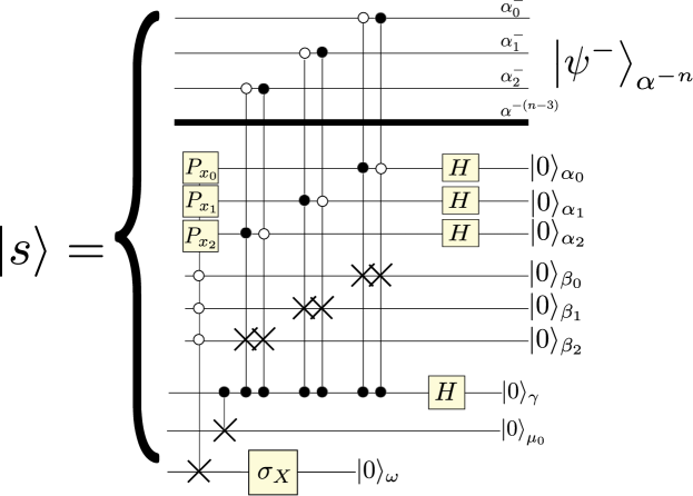
Figure 2: Circuit for generating $\left|s\right\rangle$ used in AFGA to calculate the marginal $P(x^{-3})$ of $P(x^{-n})$ evaluated at $x^{-3}=x^{3}$.

We want all horizontal lines in Fig.2 to represent qubits, except for the thick line labelled $\alpha^{-(n-3)}$ which represents $n-3$ qubits. Let $\alpha^{-}=\alpha^{-n}$, $\alpha=\alpha^{3}$, and $\beta=\beta^{3}$. Note that in the qMobius case, the number of $\alpha^{-}$, $\alpha$, $\beta$ qubits were all the same, whereas in this case, there are $n$ $\alpha^{-}$ qubits but only $3$ $\alpha$ and $\beta$ ones.

Given $x^{3}\in Bool^{3}$, define

$$T(\alpha^{-},\alpha,\beta)=\prod_{j=0}^{2}\left\{\sigma_{X}(\beta_{j})^{P_{1}(\alpha^{-}_{j})P_{0}(\alpha_{j})+P_{0}(\alpha^{-}_{j})P_{1}(\alpha_{j})}H(\alpha_{j})\right\}\;,$$ (77)

$$\pi(\alpha)=\prod_{j=0}^{2}P_{x_{j}}(\alpha_{j})\;,$$ (78)

and

$$\pi(\beta)=\prod_{j=0}^{2}P_{0}(\beta_{j})\;.$$ (79)

Our method for calculating the marginal $P(x^{-3})$ of $P(x^{-n})$ evaluated at $x^{-3}=x^{3}$ consists of applying the algorithm AFGA of Ref.[4] in the way that was described in Ref.[5], using the techniques of targeting two hypotheses and blind targeting. As in Ref.[5], when we apply AFGA in this section, we will use a sufficient target $\left|0\right\rangle_{\omega}$. All that remains for us to do to fully specify our circuit for calculating $P(x^{3})$ is to give a circuit for generating $\left|s\right\rangle$.

A circuit for generating $\left|s\right\rangle$ is given by Fig. 2. Fig.2 is equivalent to saying that

$$\left|s\right\rangle_{\mu,\nu,\omega}=\sigma_{X}(\omega)^{\pi(\beta)\pi(\alpha)}\frac{1}{\sqrt{2}}\left[\begin{array}[]{l}T(\alpha^{-},\alpha,\beta)\begin{array}[]{l}\left|\psi^{-}\right\rangle_{\alpha^{-}}\\ \left|0^{3}\right\rangle_{\alpha}\\ \left|0^{3}\right\rangle_{\beta}\end{array}\\ \left|1\right\rangle_{\gamma}\\ \left|1\right\rangle_{\mu_{0}}\\ \left|1\right\rangle_{\omega}\end{array}+\begin{array}[]{l}\left|\psi^{-}\right\rangle_{\alpha^{-}}\\ H^{\otimes 3}\left|0^{3}\right\rangle_{\alpha}\\ \left|0^{3}\right\rangle_{\beta}\\ \left|0\right\rangle_{\gamma}\\ \left|0\right\rangle_{\mu_{0}}\\ \left|1\right\rangle_{\omega}\end{array}\right]\;.$$ (80)

Claim 2

$$\left|s\right\rangle_{\mu,\nu,\omega}=\begin{array}[]{c}z_{1}\left|\psi_{1}\right\rangle_{\mu}\\ \left|1\right\rangle_{\nu}\\ \left|0\right\rangle_{\omega}\end{array}+\begin{array}[]{c}z_{0}\left|\psi_{0}\right\rangle_{\mu}\\ \left|0\right\rangle_{\nu}\\ \left|0\right\rangle_{\omega}\end{array}+\begin{array}[]{c}\left|\chi\right\rangle_{\mu,\nu}\\ \left|1\right\rangle_{\omega}\end{array}\;,$$ (81)

for some unnormalized state $\left|\chi\right\rangle_{\mu,\nu}$, where

$$\begin{array}[]{|c|c|}\hline\cr\left|\psi_{1}\right\rangle_{\mu}=\frac{1}{\sqrt{P(x^{3})}}\sum_{x^{-n}}\theta(x^{3}=x^{-3})A^{-}(x^{-n})\begin{array}[]{l}\left|x^{-n}\right\rangle_{\alpha^{-}}\\ \left|x^{3}\right\rangle_{\alpha}\\ \left|1\right\rangle_{\mu_{0}}\end{array}&\left|\psi_{0}\right\rangle_{\mu}=\begin{array}[]{l}\left|\psi^{-}\right\rangle_{\alpha^{-}}\\ \left|x^{3}\right\rangle_{\alpha}\\ \left|0\right\rangle_{\mu_{0}}\end{array}\\ \left|1\right\rangle_{\nu}=\left[\begin{array}[]{r}\left|0^{3}\right\rangle_{\beta}\\ \left|1\right\rangle_{\gamma}\end{array}\right]&\left|0\right\rangle_{\nu}=\left[\begin{array}[]{r}\left|0^{3}\right\rangle_{\beta}\\ \left|0\right\rangle_{\gamma}\end{array}\right]\\ \hline\cr\end{array}\;,$$ (82)

$$z_{1}=\frac{1}{\sqrt{2^{4}}}\sqrt{P(x^{3})}\;,$$ (83)

$$z_{0}=\frac{1}{\sqrt{2^{4}}}\;,$$ (84)

$$\frac{|z_{1}|}{|z_{0}|}=\sqrt{\frac{P(1)}{P(0)}}\;.$$ (85)

proof:

Recall that for any quantum systems $\alpha$ and $\beta$, any unitary operator $U(\beta)$ and any projection operator $\pi(\alpha)$, one has

$$U(\beta)^{\pi(\alpha)}=(1-\pi(\alpha))+U(\beta)\pi(\alpha)\;.$$ (86)

Applying identity Eq.(86) with $U=\sigma_{X}(\omega)$ yields:

$$\left|s\right\rangle = \sigma_{X}(\omega)^{\pi(\beta)\pi(\alpha)}\left|s^{\prime}\right\rangle$$ (87)

$$= \sigma_{X}(\omega)\pi(\beta)\pi(\alpha)\left|s^{\prime}\right\rangle+\begin{array}[]{l}\left|\chi\right\rangle_{\mu,\nu}\\ \left|1\right\rangle_{\omega}\end{array}$$ (90)

$$= \frac{1}{\sqrt{2}}\left[\begin{array}[]{l}\pi(\beta)\pi(\alpha)T(\alpha^{-},\alpha,\beta)\begin{array}[]{l}\left|\psi^{-}\right\rangle_{\alpha^{-}}\\ \left|0^{3}\right\rangle_{\alpha}\\ \left|0^{3}\right\rangle_{\beta}\end{array}\\ \left|1\right\rangle_{\gamma}\\ \left|1\right\rangle_{\mu_{0}}\\ \left|0\right\rangle_{\omega}\end{array}+\begin{array}[]{l}\left|\psi^{-}\right\rangle_{\alpha^{-}}\\ \frac{1}{\sqrt{2^{3}}}\left|x^{3}\right\rangle_{\alpha}\\ \left|0^{3}\right\rangle_{\beta}\\ \left|0\right\rangle_{\gamma}\\ \left|0\right\rangle_{\mu_{0}}\\ \left|0\right\rangle_{\omega}\end{array}\right]+\begin{array}[]{l}\left|\chi\right\rangle_{\mu,\nu}\\ \left|1\right\rangle_{\omega}\end{array}\;.$$ (106)

Applying identity Eq.(86) with $U=\sigma_{X}(\beta_{j})$ yields:

$$\pi(\beta)\pi(\alpha)T(\alpha^{-},\alpha,\beta)\begin{array}[]{l}\left|\psi^{-}\right\rangle_{\alpha^{-}}\\ \left|0^{3}\right\rangle_{\alpha}\\ \left|0^{3}\right\rangle_{\beta}\end{array}=$$ (110)

$$= \sum_{x^{-n}}\begin{array}[]{l}\\ \scriptstyle\left|x^{-(n-3)}\right\rangle_{\alpha^{-(n-3)}}\\ \scriptstyle\left|0^{3}\right\rangle_{\beta}\end{array}\prod_{j=0}^{2}\left\{\begin{array}[]{r}\\ \scriptstyle P_{x_{j}}(\alpha_{j})\end{array}\left[\begin{array}[]{r}\scriptstyle 1-P_{0}(\alpha^{-}_{j})P_{1}(\alpha_{j})\\ \scriptstyle-P_{1}(\alpha^{-}_{j})P_{0}(\alpha_{j})\end{array}\right]\begin{array}[]{r}\scriptstyle\left|x^{-}_{j}\right\rangle_{\alpha^{-}_{j}}\\ \scriptstyle H(\alpha_{j})\left|0\right\rangle_{\alpha_{j}}\end{array}\right\}\scriptstyle\left\langle x^{-n}|\psi^{-}\right\rangle_{\alpha^{-}}$$ (120)

$$= \begin{array}[]{r}\\ \\ \left|0^{3}\right\rangle_{\beta}\end{array}\sum_{x^{-n}}\begin{array}[]{l}A^{-}(x^{-n})\left|x^{-n}\right\rangle_{\alpha^{-}}\\ \left|x^{3}\right\rangle_{\alpha}\end{array}\prod_{j=0}^{2}C(x^{-}_{j},x_{j})\;,$$ (126)

where

$$C(x^{-}_{j},x_{j}) = \begin{array}[]{l}\left\langle x^{-}_{j}\right|_{\alpha^{-}_{j}}\\ \left\langle x_{j}\right|_{\alpha_{j}}\end{array}[P_{1}(\alpha^{-}_{j})P_{1}(\alpha_{j})+P_{0}(\alpha^{-}_{j})P_{0}(\alpha_{j})]\begin{array}[]{r}\left|x^{-}_{j}\right\rangle_{\alpha^{-}_{j}}\\ H(\alpha_{j})\left|0\right\rangle_{\alpha_{j}}\end{array}$$ (131)

$$= \frac{1}{\sqrt{2}}\begin{array}[]{l}\left\langle x^{-}_{j}\right|_{\alpha^{-}_{j}}\\ \left\langle x_{j}\right|_{\alpha_{j}}\end{array}[P_{1}(\alpha^{-}_{j})P_{1}(\alpha_{j})+P_{0}(\alpha^{-}_{j})P_{0}(\alpha_{j})]\begin{array}[]{l}\left|x^{-}_{j}\right\rangle_{\alpha^{-}_{j}}\\ \left|x_{j}\right\rangle_{\alpha_{j}}\end{array}$$ (136)

$$= \frac{1}{\sqrt{2}}\theta(x_{j}=x^{-}_{j})\;.$$ (137)

QED

References

• [1] R. Kennes, P. Smets, “Computational aspects of the Mobius transform”, arXiv:1304.1122
• [2] M. Koivisto, and K. Sood, “Exact Bayesian structure discovery in Bayesian networks”, The Journal of Machine Learning Research 5 (2004): 549-573.
• [3] Lov K. Grover, “Quantum computers can search rapidly by using almost any transformation”, arXiv:quant-ph/9712011
• [4] R.R. Tucci, “An Adaptive, Fixed-Point Version of Grover’s Algorithm”, arXiv:1001.5200
• [5] R.R. Tucci, “Quantum Circuit for Calculating Symmetrized Functions Via Grover-like Algorithm”, arXiv:1403.6707
• [6] R.R. Tucci, “Code Generator for Quantum Simulated Annealing”, arXiv:0908.1633
• [7] G. Brassard, P. Hoyer, M. Mosca, and A. Tapp, “Quantum amplitude amplification and estimation”, arXiv:quant-ph/0005055
• [8] C. Dürr, P. Hoyer, “A quantum algorithm for finding the minimum”, arXiv:quant-ph/9607014.
• [9] G. Brassard, F. Dupuis, S. Gambs, and A. Tapp, “An optimal quantum algorithm to approximate the mean and its application for approximating the median of a set of points over an arbitrary distance”, arXiv:1106.4267