Degenerate groundstates and multiple bifurcations in a two-dimensional $q$-state quantum Potts model

Abstract

We numerically investigate the two-dimensional $q$-state quantum Potts model on the infinite square lattice by using the infinite projected entangled-pair state (iPEPS) algorithm. We show that the quantum fidelity, defined as an overlap measurement between an arbitrary reference state and the iPEPS groundstate of the system, can detect $q$-fold degenerate groundstates for the $Z_{q}$ broken-symmetry phase. Accordingly, a multiple-bifurcation of the quantum groundstate fidelity is shown to occur as the transverse magnetic field varies from the symmetry phase to the broken-symmetry phase, which means that a multiple-bifurcation point corresponds to a critical point. A (dis-)continuous behavior of quantum fidelity at phase transition points characterizes a (dis-)continuous phase transition. Similar to the characteristic behavior of the quantum fidelity, the magnetizations, as order parameters, obtained from the degenerate groundstates exhibit multiple bifurcation at critical points. Each order parameter is also explicitly demonstrated to transform under the subgroup of the $Z_{q}$ symmetry group. We find that the $q$-state quantum Potts model on the square lattice undergoes a discontinuous (first-order) phase transition for $q=3$ and $q=4$, and a continuous phase transition for $q=2$ (the 2D quantum transverse Ising model).

I Introduction

Most quantum phase transitions sachdev in quantum many-body physics can be understood within the Landau-Ginzburg-Wilson paradigm which provides the fundamental key concepts of spontaneous symmetry-breaking and local order parameters. In the last decades, some of the most remarkable discoveries, such as various magnetic orderings, the integer and fractional quantum Hall effects hall1 ; hall2 and high-$T_{c}$ superconductors superconductor have brought more attention to quantum phase transitions in condensed matter physics. However, some systems do not seem to be well understood within the paradigm in characterizing newly discovered quantum states. Also, in spite of the decisive role of the key concepts in characterizing quantum phase transitions, practical and systematic ways to understand some (either explicit or implicit) broken-symmetry phases and (either local or nonlocal) order parameters have not been readily available. The crucial difficulties reside in the fact that (i) calculating groundstate wavefunctions and identifying degenerate groundstate wavefunctions are usually a formidable task, and (ii) an efficient way to determine groundstate phase diagrams is necessary.

Encouragingly, in the past few years, significant advances have been made, both in classically simulating quantum lattice systems and in determining groundstate phase diagrams iTEBD ; iPEPS ; jonas ; PHYLi . Especially, tensor network representations provide efficient quantum many-body wave functions to classically simulate quantum many-body systems iTEBD ; iPEPS ; TEBD ; MERA ; PEPS ; MPS . Tensor network algorithms in quantum lattice systems have made it possible to investigate their groundstates with an imaginary time evolution iTEBD . By using two novel approaches proposed from a quantum information perspective – entanglement Entanglement1 ; Entanglement2 ; Entanglement3 ; Entanglement4 and fidelity zhou1 ; zhou2 ; Zanardi – tensor network groundstates have been successfully implemented to determine groundstate phase diagrams of quantum lattice systems without prior knowledge of order parameters.

Although these latest advances in understanding quantum phase transitions have been achieved, directly understanding degenerate groundstates originating from spontaneous symmetry breaking and connections between a symmetry breaking and its corresponding order parameter, as the heart of the Landau-Ginzburg-Wilson theory, still remains largely unexplored. With a randomly chosen initial state subject to an imaginary time evolution, the tensor network algorithms can offer an efficient way to directly investigate degenerate groundstates in quantum lattice systems. For one-dimensional spin lattice systems, doubly degenerate ground states for broken-symmetry phases have been detected by means of the quantum fidelity bifurcations with the tensor network algorithm in various spin lattice models such as the quantum Ising model, spin-1/2 XYX model with transverse magnetic field, among others zhouzhlb ; zhwlzh ; dhzhzhou . Very recently, Su et al. Su have further demonstrated that the quantum fidelity measured by an arbitrary reference state can detect and identify explicitly all degenerate ground states ($N$-fold degenerate groundstates) due to spontaneous symmetry breaking in broken-symmetry phases for the infinite matrix product state (iMPS) representation in the one-dimensional (1D) $q$-state quantum Potts model. It has been also discussed how each order parameter calculated from degenerate ground states transforms under a subgroup of a symmetry group of the Hamiltonian.

In contrast to 1D quantum systems, however, two-dimensional (2D) quantum systems have not yet been explored to detect their degenerate ground states for broken-symmetry phases. We will thus explore the spontaneous symmetry breaking mechanism in a 2D quantum system. To describe a 2D many-body wavefunction, we will employ the infinite projected entangled-pair state (iPEPS) iPEPS ; iTEBDorus ; xiang . The infinite time-evolving block decimation (iTEBD) method iTEBD will be used to calculate iPEPS groundstate wavefunctions with randomly chosen 2D initial states. In order to distinguish degenerate groundstate wavefunctions of broken-symmetry phases and to determine phase transition points, the quantum fidelity Su , defined as an overlap measurement between an arbitrary 2D reference state and the iPEPS groundstates of the system, will be employed. The defined quantum fidelity corresponds to a projection of each 2D iPEPS groundstate onto a chosen 2D reference state. Consequently, the number of different projection magnitudes denotes the groundstate degeneracy of a system for a fixed system parameter. Also, a critical point can be noticed by the collapse of different projection magnitudes to one projection magnitude. With such a property of the quantum fidelity, the different projection magnitudes of the ground states starting from the collapse point can be called a multiple bifurcation of the quantum fidelity. Furthermore, an analysis of a relation between local observables, as order parameters, from each of degenerate groundstates can allow us to specify exactly which symmetry of the system is broken in the broken-symmetry phase.

In this paper, we consider the 2D $q$-state quantum Potts model on the infinite square lattice with a transverse magnetic field. In general, $q$-state Potts models have been shown to exhibit fundamental universality classes of critical behavior and have thus become an important testing platform for different numerical approaches in studying critical phenomena potts ; wu . It is well known that the 2D classical Potts model and its equivalent 1D quantum Potts chain are exactly solved models at the critical point baxter ; wu ; hamer . In contrast to the 1D quantum Potts model, the 2D quantum $q$-state Potts model on the square lattice has not been so well understood. However, for $q=2$ the 2D quantum transverse Ising model and the equivalent 3D classical Ising model have been widely studied via a number of different techniques (see, e.g., Refs. blote ; hamer2 ; ctmrg and references therein). For $q=3$, there appears to be only one investigation hamer_q=3 of the 2D quantum Potts model, with however, many studies of the 3D classical version of the 3-state Potts model, by Monte Carlo, series expansions etc. (see, e.g., Refs. wu ; herrmann ; nienhuis ; blote ; hamer_q=3 ; hamer2 ; ctmrg and references therein). As far as we are aware, there have been no studies of the 2D quantum $4$-state Potts model.

The classical mean-field solutions wu and the extensive computations (see, e.g., Refs. wu ; herrmann ; nienhuis ; blote ; hamer_q=3 ; hamer2 ; ctmrg and references therein) have suggested that the 3D classical $q$-state Potts model, and thus the 2D quantum $q$-state Potts model, undergo a continuous phase transition for $q\leq 2$ and a first-order phase transition for $q>2$. In this paper, for the 2D quantum $q$-state Potts model on the square lattice, from the iPEPS groundstates calculated for fixed system parameters, each of the $q$-fold degenerate groundstates due to the broken $Z_{q}$ symmetry are distinguished by means of the quantum fidelity with $q$ branches in the broken-symmetry phase. A continuous (discontinuous) property of the quantum fidelity function across the phase transition point reveals a continuous (discontinuous) quantum phase transition for $q=2$ ($q=3$ and $q=4$). The multiple bifurcation points are shown to correspond to the critical points. Also, we discuss a multiple bifurcation of local order parameters and its characteristic properties for the broken-symmetry phase. We demonstrate clearly how the order parameters from each of the degenerate ground states transform under the subgroup of the symmetry group $Z_{q}$.

This paper is organized as follows. In Sec. II, the 2D $q$-state quantum Potts model on the square lattice is defined. In Sec. III, we briefly explain the iPEPS representation and the iTEBD method in 2D square lattice systems. Section IV presents how to detect degenerate groundstates by using the quantum fidelity between the degenerate groundstates and a reference state. In Sec. V, quantum phase transitions are discussed based on multiple bifurcations and multiple bifurcation points of the quantum fidelity. In Sec. VI, we discuss the magnetizations given from the degenerate groundstates and demonstrate their relation with respect to the subgroup of the $Z_{q}$ symmetry group of the 2D $q$-state quantum Potts model on the square lattice. Our summary and concluding remarks are given in Sec. VII.

II Two-dimensional quantum $q$-state Potts model

To demonstrate detecting degenerate groundstates in 2D quantum lattice systems, we consider the $q$-state quantum Potts model solyom on an infinite square lattice in a transverse magnetic field:

$$H_{q}=-\sum_{(\vec{r},\vec{r}^{\prime})}\left(\sum_{p=1}^{q-1}M^{[\vec{r}]}_{x\;,\;p}M^{[\vec{r}^{\prime}]}_{x\;,\;q-p}\right)-\sum_{\vec{r}}\lambda M^{[\vec{r}]}_{z},$$ (1)

where $\lambda$ is the transverse magnetic field and $M^{[\vec{r}]}_{\alpha,p}$ with $p\in[1,q-1]$ ($\alpha=x,z$) are the $q$-state Potts ‘spins’ at site $\vec{r}$. The $q$-state Potts spin matrices are given by

$$M_{x,1}=\left(\begin{array}[]{cc}0&I_{q-1}\\ 1&0\end{array}\right)\mbox{~{}and~{}}M_{z}=\left(\begin{array}[]{cc}q-1&0\\ 0&-I_{q-1}\end{array}\right),$$

where $I_{q-1}$ is the $(q-1)\times(q-1)$ identity matrix and $M_{x,p}=(M_{x,1})^{p}$. $(M_{x,1})^{q}$ equals the $q\times q$ identity matrix. $(\vec{r},\vec{r}^{\prime})$ runs over all possible nearest-neighbor pairs on the square lattice.

The 2D $q$-state quantum Potts model defined in Eq. (1) is invariant with respect to the $q$-way unitary transformations, i.e.,

$$U_{m}:\left\{\begin{array}[]{ccc}M^{[\vec{r}]}_{x,p}&\rightarrow&\big{(}\omega^{p}_{q}\big{)}^{m-1}M^{[\vec{r}]}_{x,p}\\ M^{[\vec{r}]}_{z}&\rightarrow&M^{[\vec{r}]}_{z}\end{array}\right.,$$ (2)

where $\omega_{q}=\exp[i\theta]$ with characteristic angle $\theta=2\pi/q$ and $m\in[1,q]$. These unitary transformations, of the form $U_{m}H_{q}U^{\dagger}_{m}=H_{q}$, imply that the 2D $q$-state Potts model possesses a $Z_{q}$ symmetry. According to the spontaneous symmetry breaking mechanism, for the $Z_{q}$ broken-symmetry phase, the system has a $q$-fold degenerate groundstate. The $Z_{q}$ broken-symmetry phase can be characterized by the nonzero value of a local order. If $\lambda\gg 1$, Eq. (1) becomes $H_{q}\approx-\sum_{\vec{r}}M^{[\vec{r}]}_{z}$ and then the transformation in Eq. (2) is nothing but the identity transformation, i.e., $U_{m}=I_{q}$. The groundstate is non-degenerate in the $Z_{q}$ symmetry phase.

III iPEPS algorithm

To demonstrate numerically detecting the $q$-fold degenerate groundstate in the 2D $q$-state quantum Potts model, we employ the infinite projected entangled-pair state (iPEPS) algorithm iPEPS ; iTEBDorus ; xiang . Let us then briefly explain the iPEPS algorithm as follows. Consider an infinite 2D square lattice where each site is labeled by a vector $\vec{r}=(x,y)$. Each lattice site can be represented by a local Hilbert space $V^{[\vec{r}]}\cong{C}^{d}$ of finite dimension $d$. The Hamiltonian $H_{q}$ with the nearest neighbor interactions on the square lattice is invariant under shifts by one lattice site. $H_{q}=\sum_{(\vec{r},\vec{r}^{\prime})}h_{q}^{[\vec{r},\vec{r}^{\prime}]}$ can decompose as a sum of terms $h_{q}^{[\vec{r},\vec{r}^{\prime}]}$ involving pairs of nearest neighbor sites. In the infinite 2D square lattice, the state $|\Psi\rangle$ can be constructed in terms of only two tensors $A^{[x,x+2y]}$ and $B^{[x,x+2y+1]}$ with $x,y\in\mathbb{Z}$, which the state $|\Psi\rangle$ is invariant under shifts by two lattice sites. The five index tensors $A^{[\vec{r}]}_{sudlr}$ and $B^{[\vec{r^{\prime}}]}_{sudlr}$ are made up of complex numbers labeled by one physical index $s$ and the four inner indices $u$, $d$, $l$ and $r$. The physical index $s$ runs over a basis of $V^{[\vec{r}]}$ so that $s=1,\ldots,d$. Each inner index takes $D$ values as a bond dimension and connects a tensor with its nearest neighbor tensors. In the iPEPS representation, thus, one can prepare a random initial state $|\Psi(0)\rangle$ numerically.

To calculate a groundstate of the system, the idea is to use the infinite time-evolving block decimation (iTEBD) algorithm, i.e., the imaginary time evolution of the prepared initial state $|\Psi(0)\rangle$ driven by the Hamiltonian $H_{q}$, i.e., $|\Psi(\tau)\rangle={e^{-H_{q}\tau}|\Psi(0)\rangle}/||e^{-H_{q}\tau}|\Psi(0)\rangle||$ iPEPS . Using a Suzuki-Trotter expansion of the time-evolution operator $U=e^{-H_{q}\tau}$ suzuki , and then updating the tensors as $A^{\prime[\vec{r}]}_{sudlr}$ and $B^{\prime[\vec{r^{\prime}}]}_{sudlr}$ after applying each of these extended operators leads to an iPEPS groundstate of the system $H_{q}$ for a large enough $\tau$. For a time slice, the evolution procedure has a contraction process in order to get the effective environment for a pair of the tensors $A$ and $B$ iPEPS ; iTEBDorus . Practically, a sweep technique  TI_MPS , originally devised for an MPS algorithm applied to one-dimensional quantum systems with periodic boundary conditions  PBC_MPS , can be used to compute two updated tensors $A^{\prime}$ and $B^{\prime}$. After the time-slice evolution, then, all the tensors are updated. This procedure is repeatedly performed until the system energy converges to a ground-state energy that yields a groundstate wave function in the iPEPS representation.

IV degenerate groundstates and quantum fidelity

Once one obtains an iPEPS ground state $|\psi^{(n)}\rangle$ with the $n$th randomly chosen initial state, one can define a quantum fidelity $F(|\psi^{(n)}\rangle,|\phi\rangle)=|\langle\psi^{(n)}|\phi\rangle|$ between the groundstate and a chosen reference state $|\phi\rangle$. Actually, $F(|\psi^{(n)}\rangle,|\phi\rangle)$ means a projection of $|\psi^{(n)}\rangle$ onto $|\phi\rangle$. If the system has only one ground state for the parameters, the projection value $F(|\psi^{(n)}\rangle,|\phi\rangle)$ has only one constant value with the random initial states. If $F(|\Psi^{(n)}\rangle,|\phi\rangle)$ has $n$ projection values with the random initial states, the system must have $n$ degenerate ground states for the fixed system parameters. With different initial states for a fixed system parameter, one can then determine how many ground states exist from how many projection values exist.

For our numerical calculation, we choose the numerical reference state $|\phi\rangle$ randomly. The quantum fidelity $F(|\psi^{(n)}\rangle,|\phi\rangle)$ asymptotically scales as $F(|\psi^{(n)}\rangle,|\phi\rangle)\sim d^{L}$, where $L=L_{x}\times L_{y}$ is the size of the two-dimensional square lattice. In Ref. zhou1 ; zhouzhlb ; zhwlzh ; dhzhzhou ; Su ; Zhou08 , the fidelity per lattice site (FLS) is defined as

$$\ln d(|\psi^{(n)}\rangle,|\phi\rangle)=\lim_{L\rightarrow\infty}\frac{1}{L}\ln F(|\psi^{(n)}\rangle,|\phi\rangle).$$ (3)

The FLS is well defined in the thermodynamic limit, even if $F$ becomes trivially zero. The FLS is within the range $0\leq d(|\psi^{(n)}\rangle,|\phi\rangle)\leq 1$. If $|\psi^{(n)}\rangle=|\phi\rangle$ then $d=1$. Within the iPEPS approach, the FLS is given by the largest eigenvalue of the transfer matrix Zhou08 . In this section, we will demonstrate explicitly how to detect degenerate groundstates of the 2D $q$-state quantum Potts model by means of the quantum fidelity in Eq. (3).

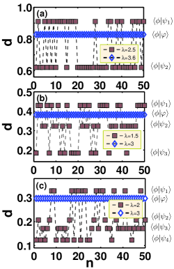
Figure 1: (color online) Groundstate quantum fidelity per site $d$ for (a) the quantum Ising model, (b) the quantum three-state Potts model and (c) the quantum four-state Potts model on the square lattice with an arbitrary reference state as a function of random initial state trials $n$. Here, an arbitrary reference state $|\phi\rangle$ is chosen numerically. The numerical iPEPS groundstates $|\psi\rangle$ are in the broken symmetry phase with transverse coupling (a) $\lambda=2.5$, (b) $\lambda=1.5$ and (c) $\lambda=2$. The state $|\varphi\rangle$ is in the symmetry phase with (a) $\lambda=3.6$, (b) $\lambda=3.0$ and (c) $\lambda=3.0$. Note that (a) two, (b) three and (c) four different values of the fidelity indicate that there are (a) two, (b) three and (c) four degenerate ground states in the symmetry broken phase.

To begin, we choose $\lambda=2.5$ and $3.6$ for the quantum Ising model ($q=2$), $\lambda=1.5$ and $3.0$ for the three-state quantum Potts model ($q=3$), and $\lambda=2.0$ and $3.0$ for the four-state quantum Potts model ($q=4$). For each given $\lambda$, the iPEPS goundstates are calculated with fifty different randomly chosen initial states, i.e., $n=50$. To calculate the FLS $d$, the arbitrary numerical reference state $|\phi\rangle$ is also chosen randomly. In Fig. 1, we plot the FLS $d$ as a function of the random initial states for (a) $q=2$, (b) $q=3$ and (c) $q=4$. For the Ising model, Fig. 1(a) shows that there are two different values of the FLS for $\lambda=2.5$, while there exists only one value of the FLS for $\lambda=3.6$. This implies that, for $\lambda=2.5$, the Ising model system is in the $Z_{2}$ broken-symmetry phase, while the system is in the symmetry phase for $\lambda=3.6$. We label the two degenerate groundstates by $|\psi_{1}\rangle$ and $|\psi_{2}\rangle$ for each value of the FLS for $\lambda=2.5$. For $\lambda=3.6$ the groundstate is denoted by $|\varphi\rangle$.

For the three-state Potts model, Fig. 1(b) shows that there are three different values of the FLS for $\lambda=1.5$, while there is only one value of the FLS for $\lambda=3.0$. Thus, for $\lambda=1.5$, the three-state Potts model is in the $Z_{3}$ broken-symmetry phase, while the system is in the symmetry phase for $\lambda=3.0$. We label the three degenerate groundstates from each value of the FLS for $\lambda=1.5$ by $|\psi_{1}\rangle$, $|\psi_{2}\rangle$ and $|\psi_{3}\rangle$. For $\lambda=3.0$, the groundstate is denoted by $|\varphi\rangle$ in the symmetry phase.

Consistently, one may expect that there are four degenerate groundstates in the $Z_{4}$ broken-symmetry phase while there exists only one groundstate in the symmetry phase. Indeed, for $q=4$, Fig. 1(c) shows the four degenerate groundstates for $\lambda=2.0$ and the one groundstate for $\lambda=3.0$. Athough we have demonstrated how to detect all of the degenerate groundstates only for the cases $q=2$, $q=3$ and $q=4$ in this study, one may detect $q$-fold degenerate groundstates in the 2D $q$-state quantum Potts model on the infinite square lattice for any $q$. Also, the above results imply that the phase transition points $\lambda_{c}$ should exist between (a) $\lambda=2.5$ and $\lambda=3.6$ for the Ising model, (b) $\lambda=1.5$ and $\lambda=3.0$ for the three-state Potts model, and (c) $\lambda=2.0$ and $\lambda=3.0$ for the four-state Potts model. The nature of the phase transitions will be discussed in the next section.

In order to ensure that we detect all degenerate groundstates, we have chosen over fifty random initial states for each $q$. The probability $P_{q}(n)$ that the system is in each groundstate for the broken-symmetry phase is shown to be $P_{2}(n)\simeq 1/2$ (Ising model), $P_{3}(n)\simeq 1/3$ (three-state Potts model) and $P_{4}(n)\simeq 1/4$ (four-state Potts model) in the broken-symmetry phase. For given $q$, then, with a large number of random initial state trials, one may detect the $q$ degenerate iPEPS groundstates with the probability $P_{q}(n\rightarrow\infty)=1/q$ for finding each degenerate groundstate in the $Z_{q}$ broken-symmetry phase. Consequently, in the 2D $q$-state quantum Potts model on the infinite square lattice, it is shown that all of the $q$-fold degenerate states for the $Z_{q}$ broken-symmetry phase can be detected by using the quantum fidelity with an arbitrary reference state in Eq. (3).

V Multiple-bifurcations of the FLS and phase transitions

In the Landau-Ginzburg-Wilson paradigm for quantum phase transitions, as is well-known, spontaneous symmetry breaking leads to a system having degenerate groundstates in its broken-symmetry phase. This means that the degenerate groundstates in the broken-symmetry phase exist until the system reaches its phase boundaries, i.e., its phase transition point. In the $q$-state quantum Potts model, the $q$-fold degenerate groundstates for the broken-symmetry phases become one groundstate at phase transition points. From the perspective of quantum fidelity, the $q$ different values of the FLS, which indicate the $q$ different degenerate groundstates, should collapse into one value of the FLS at a phase transition point.

In order to see such expected behavior of the FLS, we have detected the iPEPS degenerate groundstates by varying the transverse magnetic field $\lambda$. From the detected iPEPS degenerate groundstates, we plot the FLS as a function of $\lambda$ for $q=2$, $3$ and $4$ in Fig. 2. Figure 2 shows clearly that, as the transverse magnetic field decreases, the single value of the FLS in the broken-symmetry phase branches into $q$ values. The branch points of the FLS are estimated numerically to be $\lambda=3.23$ for $q=2$, $\lambda=2.616$ for $q=3$ and $\lambda=2.43$ for $q=4$ (cf Fig. 2). In fact, the branch points are expected to be the phase transition points obtained from the local order parameters, which will be shown in the next section. Such branching behavior of the FLS can be called multiple bifurcation and such a branch point a multiple bifurcation point.

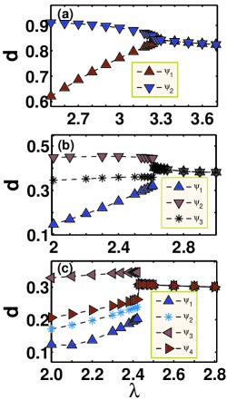
y

Figure 2: (color online) Groundstate quantum fidelity per site $d$ for (a) the quantum Ising model, (b) the quantum three-state Potts model and (c) the quantum four-state Potts model as a function of the transverse magnetic field $\lambda$ with the truncation dimension (a) $\chi=4$, (b) $\chi=6$ and (c) $\chi=4$. In the broken symmetry phase, the $q$ branches of the FLS correspond to the $q$ degenerate groundstates. As the magnetic field crosses the critical point $\lambda_{c}$, the FLS shows multiple bifurcations with (a) two, (b) three and (c) four branches in the broken symmetry phase.

Moreover, it should be noted that for $q=2$ (the Ising model) the branching is continuous, while for $q=3$ and $q=4$ the branching is abrupt. Such continuous (discontinuous) behavior of the FLS indicates a continuous (discontinuous) phase transition. As a result, the FLS in Eq. (3) can distinguish between continuous and discontinuous quantum phase transitions. In this way the $q$-state quantum Potts model on the square lattice undergoes a continuous (discontinuous) phase transition for $q\leq 2$ ($q>2$).

As already mentioned, we have chosen several reference states for the quantum fidelity calculation. Any randomly chosen reference state except for the system groundstates gives the same number of groundstates and the same critical point, though the amplitudes of the quantum fidelity depend on a chosen reference state. Consequently, it has been demonstrated that the quantum fidelity between degenerate groundstates and an arbitrary reference state can detect a critical point. However, it should be stressed that our emphasis here is not in obtaining accurate estimates for the critical points $\lambda_{c}$. Rather our emphasis is on the general framework for detecting degenerate groundstates in a 2D quantum system using quantum fidelity to determine continuous or discontinuous phase transitions due to a spontaneous symmetry breaking. Indeed, the estimate $\lambda_{c}\sim 3.23$ obtained for the critical point of the quantum transverse Ising model on the square lattice compares rather poorly with the most accurate current estimate $\lambda_{c}=3.044$, obtained using quantum Monte Carlo blote . For this model, previous studies using iPEPS yield estimates of 3.06 iPEPS and 3.04 ctmrg , where the latter estimate involves a modification using the corner transfer matrix renormalization group. For the three-state quantum Potts model on the square lattice, the estimate $\lambda_{c}\sim 2.616$ is closer to the known estimate $\lambda_{c}\sim 2.58$ hamer_q=3 . As far as we are aware, there are no other estimates to compare with our result $\lambda_{c}\sim 2.43$ for the four-state quantum Potts model on the square lattice. We note that in each case our estimates could be improved by using a more refined updating scheme in the iPEPS algorithm, rather than the simplified updating scheme used.

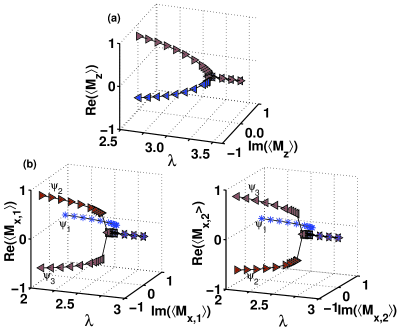
Figure 3: (color online) Magnetization (a) $\langle M_{z}\rangle$ as a function of the transverse magnetic field $\lambda$ for the quantum Ising model obtained with truncation dimension $\chi=4$. The critical point is estimated to be at $\lambda_{c}=3.23$. Magnetization (b) (left panel) $M_{x,1}$ and (b) (right panel) $M_{x,2}$ as a function of the transverse magnetic field $\lambda$ for the quantum three-state Potts model obtained with truncation dimension $\chi=6$. The critical point is estimated to be at $\lambda_{c}=2.616$.

VI Order parameters

According to the Landau theory of spontaneous symmetry breaking, a broken-symmetry phase is characterized by nonzero values of a local observable – the local order parameter. As discussed Su , spontaneous symmetry breaking leads to a degenerate groundstate for the broken-symmetry phase. Consequently, the relations between the local order parameters calculated from degenerate groundstates are determined by a symmetry group of the system Hamiltonian. Here we will show a relation between the local order parameters within the subgroup of the symmetry group of the system Hamiltonian.

Let us first discuss the local magnetization for the quantum Ising model. In Fig. 3(a), we plot the magnetization $\langle M_{x}\rangle_{m}$ as a function of the traverse magnetic field $\lambda$. The magnetizations disappear gradually to zero at the numerical critical point $\lambda_{c}$. For the broken-symmetry phase $\lambda<\lambda_{c}$, the magnetization is calculated from each of the two degenerate groundstates, where each groundstate wavefunction is denoted by $|\psi_{m}\rangle$, with $m\in\{1,2\}$. The magnetizations are related to each other by $\langle M_{x}\rangle_{1}=-\langle M_{x}\rangle_{2}$. Then, for a given magnetic field, the relation between the two magnetizations in the complex magnetization plane can be regarded as a rotation characterized by the value $\omega_{2}=\exp[2\pi i/2]$, i.e., $\langle M_{x}\rangle_{1}=\omega^{-1}_{2}\langle M_{x}\rangle_{2}$. The two degenerate groundstates give the same value for the $z$-component magnetizations, i.e., $\langle M_{z}\rangle_{1}=\langle M_{z}\rangle_{2}$. This implies that the Ising model Hamiltonian is invariant under the unitary transformations $U_{1}=I$ and $U_{2}$ in Eq. (2), but (as expected) the two degenerate groundsates are not invariant under the unitary transformation $U_{2}$ in the $Z_{2}$ broken-symmetry phase. Thus, the characteristic rotation angles between the different magnetizations are $\theta=0$ and $\theta=\pi$. The relation between the magnetizations can be written as $\langle M_{x}\rangle_{m}=g_{2}\langle M_{x}\rangle_{m^{\prime}}$ with $g_{2}\in\{I,\omega_{2}\}$. Further, the magnetizations are shown to exhibit a bifurcation behavior, similar to the FLS. The continuous behavior of the two magnetizations also shows that the phase transition is continuous.

For the three-state quantum Potts model, in Fig. 3(b), we display the magnetizations $\langle M_{x,1}\rangle$ and $\langle M_{x,2}\rangle$ as a function of the traverse magnetic field. Note that all of the absolute values of the magnetizations $\langle\psi_{m}|M_{x,p}|\psi_{m}\rangle\equiv\langle M_{x,p}\rangle_{m}$ are the same at a given magnetic field $\lambda$. Here, we have chosen the state $|\psi_{1}\rangle$ that gives a real value of the magnetization, i.e., $\langle M_{x,1}\rangle_{1}$ and $\langle M_{x,2}\rangle_{1}$ are real. In contrast to the quantum Ising model, all of the magnetizations disappear abruptly to zero at the critical point $\lambda_{c}$, which indicates that the phase transition is a discontinuous. For the broken-symmetry phase $\lambda<\lambda_{c}$, the magnetization is calculated from each the three degenerate groundstates denoted by $|\psi_{m}\rangle$. For a given magnetic field, the magnetizations in the complex magnetization plane are related with a characteristic rotation $\omega_{3}=\exp[2\pi i/3]$. Actually in Fig. 3(b) it is observed that the magnetizations are related to one another by $\langle M_{x,1}\rangle_{1}=\omega^{-1}_{3}\langle M_{x,1}\rangle_{2}=\omega^{-2}_{3}\langle M_{x,1}\rangle_{3}$ and $\langle M_{x,2}\rangle_{1}=\omega^{-2}_{3}\langle M_{x,2}\rangle_{2}=\omega^{-4}_{3}\langle M_{x,2}\rangle_{3}$. Each groundstate wavefunction gives the relations $\langle M_{x,1}\rangle_{1}=\langle M_{x,2}\rangle_{1}$, $\langle M_{x,1}\rangle_{2}=\omega^{-1}_{3}\langle M_{x,2}\rangle_{2}$ and $\langle M_{x,1}\rangle_{3}=\omega^{-2}_{3}\langle M_{x,2}\rangle_{3}$. The three degenerate groundstates also give the same value for the $z$-component magnetizations, i.e., $\langle M_{z}\rangle_{1}=\langle M_{z}\rangle_{2}=\langle M_{z}\rangle_{3}$. These imply that the three-state quantum Potts model Hamiltonian is invariant under the unitary transformations $U_{1}=I$, $U_{2}$ and $U_{3}$ with $\omega_{3}=\exp[2\pi i/3]$ in Eq. (2), but the three degenerate groundsates are not invariant under the unitary transformations $U_{2}$ and $U_{3}$ in the $Z_{3}$ broken-symmetry phase. Thus the characteristic magnetization rotation angles are $\theta=0$, $2\pi/3$ and $4\pi/3$. The magnetizations obey the relations $\langle M_{x,p}\rangle_{m}=g_{3}\langle M_{x,p^{\prime}}\rangle_{m^{\prime}}$ with $g_{3}\in\{I,\omega_{3},\omega^{2}_{3}\}$.

Based on the above relations between the magnetizations for $q=2$ and $q=3$, we can infer a general relation between the magnetizations for the $q$-state quantum Potts model on the square lattice. For any $q$, the relations are given by

$$\langle M_{x,p}\rangle_{m} = \omega^{p^{\prime}(1-m^{\prime})-p(1-m)}_{q}\langle M_{x,p^{\prime}}\rangle_{m^{\prime}},$$ (4a)

$$\langle M_{z}\rangle_{m} = \langle M_{z}\rangle_{m^{\prime}}.$$ (4b)

The magnetizations $M_{x,p}$ with respect to a different degenerate groundstate (i.e., $p=p^{\prime}$) satisfy $\langle M_{x,p}\rangle_{m}=\omega^{p(m-m^{\prime})}_{q}\langle M_{x,p}\rangle_{m^{\prime}}$ as deduced from Eq. (4). For one of the degenerate groundstate wavefunction (i.e., $m=m^{\prime}$), the magnetizations of the operators $M_{x,1},\ldots,M_{x,q-2}$ and $M_{x,q-1}$ satisfy $\langle M_{x,p}\rangle_{m}=\omega^{(p^{\prime}-p)(1-m)}_{q}\langle M_{x,p^{\prime}}\rangle_{m}$ as deduced from Eq. (4). These results show that, in the complex magnetization plane, the rotations between the magnetizations for a given magnetic field are determined by the characteristic rotation angles $\theta=0,2\pi/q,4\pi/q,\ldots,2(q-1)\pi/q$. As a result, the relations between the order parameters in Eq. (4a) can be rewritten as

$$\langle M_{x,p}\rangle_{m} = g_{q}\langle M_{x,p^{\prime}}\rangle_{m^{\prime}},$$ (5a)

$$g_{q} \in \{I,\omega_{q},\omega^{2}_{q},\cdots,\omega^{q-1}_{q}\}.$$ (5b)

Equation (5) shows clearly that the 2D $q$-state quantum Potts model on the square lattice has the discrete symmetry group $Z_{q}$ consisting of $q$ elements.

Figure 4: (color online) Magnetization (a) $\langle M_{x,1}\rangle$, (b) $\langle M_{x,2}\rangle$ and (c) $\langle M_{x,3}\rangle$ as a function of the transverse magnetic field $\lambda$ for the quantum four-state Potts model obtained with truncation dimension $\chi=4$. For the broken symmetry phase the magnetizations follow from each of the four degenerate groundstates. The critical point is estimated to be at $\lambda_{c}=2.43$.

One can show that the characteristic relations between the magnetizations in Eqs. (4) and (5) hold for the four-state quantum Potts model. In Fig. 4 we plot the magnetizations $\langle M_{x,1}\rangle$, $\langle M_{x,2}\rangle$ and $\langle M_{x,3}\rangle$ as a function of the traverse magnetic field $\lambda$. The magnetizations indicate that the phase transition is discontinuous. Also, the absolute values of the magnetizations have the same values at a given magnetic field and the magnetizations in the complex magnetization plane have a relation between them under rotation characterized by the value $\omega_{4}=\exp[2\pi i/4]$. The degenerate groundstates give the same values $\langle M_{z}\rangle_{1}=\langle M_{z}\rangle_{2}=\langle M_{z}\rangle_{3}=\langle M_{z}\rangle_{4}$ for the $z$-component magnetizations.

In Fig. 4, we also observe that for a given magnetic field $\lambda<\lambda_{c}$, the relations between the magnetizations are $\langle M_{x,1}\rangle_{1}=\omega^{-1}_{4}\langle M_{x,1}\rangle_{2}=\omega^{-2}_{4}\langle M_{x,1}\rangle_{3}=\omega^{-3}_{4}\langle M_{x,1}\rangle_{4}$ from Fig. 4(a), $\langle M_{x,2}\rangle_{1}=\omega^{-2}_{4}\langle M_{x,2}\rangle_{2}=\omega^{-4}_{4}\langle M_{x,2}\rangle_{3}=\omega^{-6}_{4}\langle M_{x,2}\rangle_{4}$ from Fig. 4(b) and $\langle M_{x,3}\rangle_{1}=\omega^{-3}_{4}\langle M_{x,3}\rangle_{2}=\omega^{-6}_{4}\langle M_{x,3}\rangle_{3}=\omega^{-9}_{4}\langle M_{x,3}\rangle_{4}$ from Fig. 4(c). Also, for each groundstate wavefunction the magnetizations obey the relations $\langle M_{x,1}\rangle_{1}=\langle M_{x,2}\rangle_{1}=\langle M_{x,3}\rangle_{1}$, $\langle M_{x,1}\rangle_{2}=\omega^{-1}_{4}\langle M_{x,2}\rangle_{2}=\omega^{-2}_{4}\langle M_{x,3}\rangle_{2}$, $\langle M_{x,1}\rangle_{3}=\omega^{-2}_{4}\langle M_{x,2}\rangle_{3}=\omega^{-4}_{4}\langle M_{x,3}\rangle_{3}$, and $\langle M_{x,1}\rangle_{4}=\omega^{-3}_{4}\langle M_{x,2}\rangle_{4}=\omega^{-6}_{4}\langle M_{x,3}\rangle_{4}$. As expected from Eqs. (4) and (5), these results show that in the complex magnetization plane the rotations between the magnetizations for a given magnetic field are determined by the characteristic rotation angles $\theta=0$, $2\pi/4$, $4\pi/4$, and $6\pi/4$, i.e., $\langle M_{x,p}\rangle_{m}=g_{4}\langle M_{x,p^{\prime}}\rangle_{m^{\prime}}$ with $g_{4}\in\{I,\omega_{4},\omega^{2}_{4},\omega^{3}_{4}\}$.

The general results in Eqs. (4) and (5) hold for any $q$ in the 2D $q$-state quantum Potts model on the square lattice. It is shown how each order parameter transforms under the subgroup for the $Z_{q}$ symmetry group in the 2D $q$-state quantum Potts model on the infinite square lattice within the spontaneous symmetry mechanism.

VII Summary

We have investigated the quantum fidelity in the two-dimensional $q$-state quantum Potts model by employing the iPEPS algorithm on the infinite square lattice. The degenerate iPEPS groundstates have been successfully detected using the quantum fidelity. We have shown (i) that each of the degenerate groundstates possesses its own order described by a corresponding order parameter – the magnetization $\langle M_{x,p}\rangle_{m}$ – in the broken-symmetry phases, (ii) that each order parameter, which is nonzero only in the broken-symmetry phases, distinguishes the ordered phase from the disordered phases, which results in the multiple bifurcation of the order parameters at the phase transition points, and (iii) further, how each order parameter transforms under the subgroup of the $Z_{q}$ symmetry group.

In line with previous studies, we found that the $q$-state quantum Potts model on the square lattice undergoes a discontinuous (first-order) phase transition for $q=3$ and $q=4$, and a continuous phase transition for the quantum Ising model ($q=2$). Consequently, we have demonstrated that (i) the multiple bifurcations of the quantum fidelity result from the spontaneous $Z_{q}$-symmetry breaking in the broken-symmetry phase, (ii) that the multiple bifurcation points of the quantum fidelity, corresponding to the multiple bifurcation of the order parameters, correspond to the phase transition points, and (iii) the (dis-)continuous behavior of the quantum fidelity indicates that the system undergoes a (dis-)continuous quantum phase transition at the multiple bifurcation points.

Our results show conclusively that the quantum fidelity can be used for detecting degenerate groundstates and phase transition points, and for determining continuous or discontinuous phase transitions due to a spontaneous symmetry breaking, without knowing any details of a broken symmetry between a broken-symmetry phase and a symmetry phase as a system parameter crosses its critical value (i.e., at a multiple bifurcation point).

- (1) S. Sachdev, Quantum Phase Transitions (Cambridge University Press, Cambridge, 1999).
- (2) R.E. Prangee and S.M. Girvin, The Quantum Hall Effect (Springer, New York, 1990).
- (3) J.K. Jain, Composite Fermions (Cambridge University Press, Cambridge, 2007).
- (4) J.G. Bednorz and K.A. Müller, Phys. B 64,189 (1986).
- (5) G. Vidal, Phys. Rev. Lett. 98, 070201 (2007).
- (6) J. Jordan, R. Orús, G. Vidal, F. Verstraete and J.I. Cirac, Phys. Rev. Lett. 101, 250602 (2008).
- (7) J.A. Kjäll, M.P. Zaletel, R.S.K. Mong, J.H. Bardarson and F. Pollmann, Phys. Rev. B 87, 235106 (2013).
- (8) P.H.Y. Li, R.E. Bishop, D.J.J. Farnell and C.E. Campbell, Phys. Rev. B 86, 144404 (2012).
- (9) G. Vidal, Phys. Rev. Lett. 91, 147902 (2003); G. Vidal, Phys. Rev. Lett. 93, 040502 (2004).
- (10) G. Vidal, Phys. Rev. Lett. 99, 220405 (2007); G. Evenbly and G.Vidal, Phys. Rev. B 79, 144108 (2009).
- (11) F. Verstraete and J.I. Cirac, arXiv:cond-mat/0407066; V. Murg, F. Verstaete, and J.I. Cirac, Phys. Rev. A 75, 033605 (2007).
- (12) M. Fannes, B. Nachtergaele, and R.F. Werner, Comm. Math. Phys. 144, 443 (1992); J. Funct. Anal. 120, 511 (1994); S. Ostlund and S. Rommer, Phys. Rev. Lett. 75, 3537 (1995).
- (13) J. Preskill, J. Mod. Opt. 47, 127 (2000).
- (14) T.J. Osborne and M.A. Nielsen, Phys. Rev. A 66, 032110; A. Osterloh, L. Amico, G. Falci and R. Fazio, Nature 416, 608 (2002)
- (15) A. Kitaev and J. Preskill, Phys. Rev. Lett. 96, 110404(2006); M. Levin and X.-G. Wen, Phys. Rev. Lett. 96, 110405 (2006).
- (16) G. Vidal, J.I. Latorre, E. Rico and A. Kitaev, Phys. Rev. Lett. 90, 227902 (2003).
- (17) H.-Q. Zhou, arXiv:0704.2945.
- (18) H.-Q. Zhou and J.P. Barjaktarevic, cond-mat/0701608.
- (19) P. Zanardi and N. Paunkovic, Phys. Rev. E 74, 031123 (2006).
- (20) H.-Q. Zhou, J.-H. Zhao and B. Li, J. Phys. A 41, 492002 (2008).
- (21) J.-H. Zhao, H.-L. Wang, B. Li and H.-Q. Zhou, Phys. Rev. E 82, 061127 (2010).
- (22) Y.-W. Dai, B.-Q. Hu and J.-H. Zhao, J. Phys. A 43, 372001 (2010); H.-L. Wang, Y.-W. Dai, B.-Q. Hu and H.-Q. Zhou, Phys. Lett. A 43, 375, 4045 (2011); J.-H. Zhao, H.-L. Wang, B. Li and H.-Q. Zhou, arXiv:0920.1669.
- (23) Y.H. Su, B.-Q. Hu, S.-H. Li and S. Y. Cho, Phys. Rev. E 88, 032110 (2013).
- (24) R. Orús and G.Vidal, Phys. Rev. B 78, 155117 (2008).
- (25) H.C. Jiang, Z.Y. Wang and T. Xiang, Phys. Rev. Lett. 101, 090603 (2008).
- (26) R.B. Potts, Proc. Cambridge Philos. Soc. 48, 106 (1952).
- (27) F.Y. Wu, Rev. Mod. Phys. 54, 235 (1982).
- (28) R.J. Baxter, J.Phys. C 6, L445 (1973).
- (29) C.J. Hamer, J. Phys. A 14, 2981 (1981).
- (30) C.J. Hamer, J. Phys. A 33, 6683 (2000).
- (31) H.W.J. Blöte and Y. Deng, Phys. Rev. E 66, 066110 (2002).
- (32) R. Orús and G.Vidal, Phys. Rev. B 80, 099403 (2009).
- (33) C.J. Hamer, M. Aydin, J. Oitmaa and H.-X. He, J. Phys. A 23, 4025 (1990).
- (34) H.J. Herrmann, Z. Phys. B 35, 171 (1979).
- (35) B. Nienhuis, E.K. Riedel and M. Schick, Phys. Rev. B 23, 6055 (1981).
- (36) J. Solyom and P. Pfeuty, Phys. Phys. B 24, 218 (1981).
- (37) M. Suzuki, Phys. Lett. A 146, 319 (1990).
- (38) D. Perez-Garcia et al., Quantum Inf. Comput. 7, 401 (2007), arXiv:quant-ph/0608197.
- (39) F. Verstraete, D. Porras and J.I. Cirac, Phys. Rev. Lett. 93, 227205 (2004).
- (40) H.-Q. Zhou, R. Orús and G. Vidal, Phys. Rev. Lett. 100, 080602 (2008).