QCD sum rules study of $X(4350)$

Abstract

The QCD sum rule approach is used to analyze the nature of the rencently observed new resonance $X(4350)$, which is assumed to be a diquark-antidiquark state $[cs][\bar{c}\bar{s}]$ with $J^{PC}=1^{-+}$. The interpolating current representing this state is proposed. In the calculation, contributions of operators up to dimension six are included in the operator product expansion (OPE), as well as terms which are linear in the strange quark mass $m_{s}$. We find $m_{1^{-+}}=(4.82\pm 0.19)\,\mbox{GeV}$, which is not compatible with the $X(4350)$ structure as a $1^{-+}$ tetraquark state. Finally, we also discuss the difference of a four-quark state’s mass whether the state’s interpolating current has a definite charge conjugation.

I Introduction

Recently, the Belle Collaboration found a new narrow structure $X(4350)$ in the $\phi J/\psi$ mass spectrum, when searching for $Y(4140)$ reported by CDF Collaboration. The mass and width of the state is $(4350.6^{+4.6}_{-5.1}\pm 0.7)\,\rm{MeV}$ and $(13.3^{+17.9}_{-9.1}\pm 4.1)\,\rm{MeV}$ bellex . Some theoretical works have been done before the Belle experiment. Wang performs a systematic study of the mass spectrum of the vector hidden charm and bottom tetraquark states using the QCD sum rules wang2 . Zhang $et$ $al.$ calculate the mass of the $D_{s}^{\ast}\bar{D}_{s}^{\ast}$ molecular state to be $(4.36\pm 0.08)\,\rm{GeV}$ Zhang . Stancu studies mass spectrum of the $[cs][\bar{c}\bar{s}]$ tetraquarks Stancu4 . Both of their results are consistent with the experimental data bellex . The possible quantum numbers for a state decaying into $\phi J/\psi$ are $J^{PC}=0^{++},~{}1^{-+}$ or $2^{++}$. Wang interprets the $X(4350)$ as a scalar $\bar{c}c$ and ${D}_{s}^{\ast}{\bar{D}}_{s}^{\ast}$ mixing state with QCD sum rules wang . In Ref. Liu0911 , Liu $et$ $al.$ discuss the possibility that the $X(4350)$ is an excited $P$-wave charmonium state $\chi_{c2}^{\prime\prime}$ by studying the strong decays of the $P$-wave charmonium states with the ${}^{3}P_{0}$ model.

Among these quantum numbers, $J^{PC}=1^{-+}$ known as exotic attracts great theoretical attention. The state considered in Ref. Zhang has $J^{P}=1^{-}$ without a definite charge conjugation. Using QCD sum rules Nielsen , Albuquerque $et$ $al.$ study a molecular state with a vector and a scalar $D_{s}$ mesons with a definite positive charge conjugation, and conclude that it is not possible to describe the $X(4350)$ structure as a $1^{-+}~{}D_{s}^{*}{D}_{s0}^{*}$ molecular state. Otherwise, Ma uses effective lagrangian approach to estimate $X(4350)$ decay, and concludes that $X(4350)$ as a $D_{s}^{*}{D}_{s0}^{*}$ can’t be ruled out Ma . Under such a circumstance, there is no definite structure with $J^{PC}=1^{-+}$ for $X(4350)$, we propose to take the $X(4350)$ as a diquark-antidiquark state with $J^{PC}=1^{-+}$. Mass property is helpful for understanding whether $X(4350)$ could be a diquark-antidiquark state with $J^{PC}=1^{-+}$. However, in low energy and hadronic scales, it is difficult to get reliable theoretical estimate for the mass using the perturbative QCD. Therefore, we need some non-perturative methods to describe the non-perturative phenomena. QCD sum rules svz ; reinders ; overview3 is powerful since they are based on the fundamental QCD lagrangian. From this perspective of view, the report NielsenPR guides practitioners to compute masses of this kind of new discovering states.

The paper is organized as follows. In Sec. II, QCD sum rule for the diquark-antidiquark tetraquark state with $J^{PC}=1^{-+}$ state is introduced, and both the phenomenological representation and QCD side are derived. In Sec.III, we present numerical analysis to extract the hadronic mass and decay constant. This section also contains a brief summary.

II the tetraquark state QCD sum rules

The lowest-dimension current interpolating a $J^{PC}=1^{-+}$ state with the symmetric spin distribution $[cs]_{S=0}[\bar{c}\bar{s}]_{S=1}+[cs]_{S=1}[\bar{c}\bar{s}]_{S=0}$ is given by

$$j_{\mu}={\epsilon_{abc}\epsilon_{dec}\over\sqrt{2}}[(s_{a}^{T}C\gamma_{5}c_{b})(\bar{s}_{d}\gamma_{\mu}\gamma_{5}C\bar{c}_{e}^{T})-(s_{a}^{T}C\gamma_{5}\gamma_{\mu}c_{b})(\bar{s}_{d}\gamma_{5}C\bar{c}_{e}^{T})]\;,$$ (1)

where $a,~{}b,~{}c,~{}...$ are color indices and $C$ is the charge conjugation matrix.

The QCD sum rule attempts to link the hadron phenomenology with the interactions of quarks and gluons, which contains three main ingredients: an approximate description of the correlator in terms of intermediate states through the dispersion relation, a description of the same correlator in terms of QCD degrees of freedom via an OPE, and a procedure for matching these two descriptions and extracting the parameters that characterize the hadronic state of interest.

The two-point correlation function is given by

$$\Pi^{\mu\nu}(q^{2})=i\int d^{4}x\mbox{e}^{iq.x}\langle 0|T[j^{\mu}(x)j^{\nu+}(0)]|0\rangle.$$ (2)

Lorentz covariance implies that the two-point correlation function can be generally parameterized as

$$\Pi^{\mu\nu}(q^{2})=(\frac{q^{\mu}q^{\nu}}{q^{2}}-g^{\mu\nu})\Pi^{(1)}(q^{2})+\frac{q^{\mu}q^{\nu}}{q^{2}}\Pi^{(0)}(q^{2}).$$ (3)

The part of the correlator proportional to $g_{\mu\nu}$ will be chosen to extract the mass sum rule, since it gets contributions only from the $1^{-+}$ state. The coupling of the current with the state can be defined by the decay constant as follows:

$$\langle 0|j_{\mu}|X\rangle = \lambda\epsilon_{\mu}.$$ (4)

In phenomenology, $\Pi^{(1)}(q^{2})$ can be expressed as a dispersion integral over a physical spectral function

$$\Pi^{(1)}(q^{2})=\frac{\lambda^{2}}{M_{X}^{2}-q^{2}}+\frac{1}{\pi}\int_{s_{0}}^{\infty}ds\frac{\mbox{Im}\Pi^{(1)\mbox{phen}}(s)}{s-q^{2}}+\mbox{subtractions},$$ (5)

where $M_{H}$ denotes the mass of the hadronic resonance. In the OPE side, $\Pi^{(1)}(q^{2})$ can be written in terms of a dispersion relation as

$$\Pi^{(1)}(q^{2})=\int_{(2m_{c}+2m_{s})^{2}}^{\infty}ds\frac{\rho^{\mbox{\scriptsize OPE}}(s)}{(s-q^{2})},$$ (6)

where the spectral density is given by

$$\rho^{\mbox{\scriptsize OPE}}(s)=\frac{1}{\pi}\mbox{Im}\Pi^{\mbox{(1)}}(s).$$ (7)

After equating the two sides, assuming quark-hadron duality, and making a Borel transformation, the sum rule can be written as

$$\lambda^{2}e^{-M_{X}^{2}/M^{2}} = \int_{(2m_{c}+2m_{s})^{2}}^{s_{0}}ds\rho^{\mbox{\scriptsize OPE}}(s)e^{-s/M^{2}}.$$ (8)

To eliminate the decay constant $\lambda$, one reckons the ratio of the derivative of the sum rule and itself, and then yields

$$M_{X}^{2} = \int_{(2m_{c}+2m_{s})^{2}}^{s_{0}}ds\rho^{\mbox{\scriptsize OPE}}se^{-s/M^{2}}/\int_{(2m_{c}+2m_{s})^{2}}^{s_{0}}ds\rho^{\mbox{\scriptsize OPE}}e^{-s/M^{2}}.$$ (9)

When calculating the OPE side, we work at the leading order in $\alpha_{s}$ and consider condensates up to dimension six, with the similar techniques in Refs. technique ; technique1 . The $s$ quark is regarded as a light one and the terms are considered up to the order of $m_{s}$. To keep the heavy-quark mass finite, one uses the momentum-space expression for the heavy-quark propagator. One calculates the light-quark part of the correlation function in the coordinate space, which is then Fourier-transformed to the momentum space in $D$ dimension. The resulting light-quark part is combined with the heavy-quark part before it is dimensionally regularized at $D=4$. For the heavy-quark propagator with two and three gluons attached, the momentum-space expressions given in Ref. reinders are used. After some tedious OPE calculations, the concrete forms of spectral densities can be derived.

$$\rho^{\mbox{\scriptsize OPE}}(s)=\rho^{\mbox{pert}}(s)+\rho^{\langle\bar{s}s\rangle}(s)+\rho^{\langle g^{2}G^{2}\rangle}(s)+\rho^{\langle g\bar{s}\sigma\cdot Gs\rangle}(s)+\rho^{\langle\bar{s}s\rangle^{2}}(s),$$

$$\rho^{\mbox{pert}}(s) = \frac{1}{3*2^{10}\pi^{6}}\int_{\alpha_{min}}^{\alpha_{max}}\frac{d\alpha}{\alpha^{3}}\int_{\beta_{min}}^{1-\alpha}\frac{d\beta}{\beta^{3}}(1-\alpha-\beta)[(\alpha+\beta)m_{c}^{2}-\alpha\beta s]^{3}$$

$${}[(5\alpha^{2}+10\alpha\beta-\alpha+5\beta^{2}-\beta+2)m_{c}^{2}-3\alpha\beta s(\alpha+\beta+1)]$$

$${}+\frac{1}{2^{8}\pi^{6}}m_{c}m_{s}\int_{\alpha_{min}}^{\alpha_{max}}\frac{d\alpha}{\alpha^{3}}\int_{\beta_{min}}^{1-\alpha}\frac{d\beta}{\beta^{2}}(1-\alpha-\beta)^{2}(\alpha+\beta)[(\alpha+\beta)m_{c}^{2}-\alpha\beta s]^{3},$$

$$\rho^{\langle\bar{s}s\rangle}(s) = \frac{\langle\bar{s}s\rangle}{2^{5}\pi^{4}}m_{c}^{2}m_{s}\int_{\alpha_{min}}^{\alpha_{max}}\frac{d\alpha}{\alpha}\int_{\beta_{min}}^{1-\alpha}\frac{d\beta}{\beta}(-3-\alpha-\beta)[(\alpha+\beta)m_{c}^{2}-\alpha\beta s]$$

$${}+\frac{\langle\bar{s}s\rangle}{2^{5}\pi^{4}}m_{c}\int_{\alpha_{min}}^{\alpha_{max}}\frac{d\alpha}{\alpha^{2}}\int_{\beta_{min}}^{1-\alpha}\frac{d\beta}{\beta^{2}}(1-\alpha-\beta)(\alpha+\beta)[(\alpha+\beta)m_{c}^{2}-\alpha\beta s]^{2}$$

$${}+\frac{\langle\bar{s}s\rangle}{2^{5}\pi^{4}}m_{s}\int_{\alpha_{min}}^{\alpha_{max}}\frac{d\alpha}{\alpha(1-\alpha)}[m_{c}^{2}-\alpha(1-\alpha)s]^{2},$$

$$\rho^{\langle g^{2}G^{2}\rangle}(s) = \frac{\langle g^{2}G^{2}\rangle}{9*2^{10}\pi^{6}}m_{c}^{4}\int_{\alpha_{min}}^{\alpha_{max}}{d\alpha}\int_{\beta_{min}}^{1-\alpha}\frac{d\beta}{\beta^{3}}(1-\alpha-\beta)^{3}$$

$${}+\frac{\langle g^{2}G^{2}\rangle}{3*2^{9}\pi^{6}}m_{c}^{3}m_{s}\int_{\alpha_{min}}^{\alpha_{max}}{d\alpha}\int_{\beta_{min}}^{1-\alpha}\frac{d\beta}{\beta^{2}}(1-\alpha-\beta)^{2}$$

$${}+\frac{\langle g^{2}G^{2}\rangle}{3*2^{9}\pi^{6}}m_{c}^{3}m_{s}\int_{\alpha_{min}}^{\alpha_{max}}d\alpha\alpha\int_{\beta_{min}}^{1-\alpha}\frac{d\beta}{\beta^{3}}(1-\alpha-\beta)^{2}$$

$${}+\frac{\langle g^{2}G^{2}\rangle}{3*2^{10}\pi^{6}}m_{c}^{2}\int_{\alpha_{min}}^{\alpha_{max}}\frac{d\alpha}{\alpha}\int_{\beta_{min}}^{1-\alpha}\frac{d\beta}{\beta^{3}}(1-\alpha-\beta)$$

$${}(3\alpha^{3}+4\alpha\beta+\beta^{2}-2\beta+1)[(\alpha+\beta)m_{c}^{2}-\alpha\beta s]$$

$${}+\frac{\langle g^{2}G^{2}\rangle}{2^{9}\pi^{6}}m_{c}m_{s}\int_{\alpha_{min}}^{\alpha_{max}}{d\alpha}\int_{\beta_{min}}^{1-\alpha}\frac{d\beta}{\beta^{3}}(1-\alpha-\beta)^{2}[(\alpha+\beta)m_{c}^{2}-\alpha\beta s],$$

$$\rho^{\langle g\bar{s}\sigma\cdot Gs\rangle}(s) =\frac{\langle g\bar{s}\sigma\cdot Gs\rangle}{3*2^{6}\pi^{4}}\int_{\alpha_{min}}^{\alpha_{max}}{d\alpha}\int_{\beta_{min}}^{1-\alpha}{d\beta}m_{c}^{2}m_{s}$$

$${}+\frac{\langle g\bar{s}\sigma\cdot Gs\rangle}{2^{6}\pi^{4}}m_{c}\int_{\alpha_{min}}^{\alpha_{max}}\frac{d\alpha}{\alpha}\int_{\beta_{min}}^{1-\alpha}\frac{d\beta}{\beta}(\alpha+\beta)[(\alpha+\beta)m_{c}^{2}-\alpha\beta s]$$

$${}+\frac{\langle g\bar{s}\sigma\cdot Gs\rangle}{3*2^{8}\pi^{4}}m_{s}\int_{\alpha_{min}}^{\alpha_{max}}{d\alpha}\int_{\beta_{min}}^{1-\alpha}\frac{d\beta}{\beta}[(\alpha+\beta)m_{c}^{2}-\alpha\beta s]$$

$${}-\frac{\langle g\bar{s}\sigma\cdot Gs\rangle}{3*2^{3}\pi^{4}}m_{c}^{2}m_{s}\sqrt{1-4m_{c}^{2}/s}$$

$${}+\frac{7\langle g\bar{s}\sigma\cdot Gs\rangle}{3*2^{6}\pi^{4}}m_{s}\int_{\alpha_{min}}^{\alpha_{max}}{d\alpha}[m_{c}^{2}-\alpha(1-\alpha)s]$$

$${}-\frac{\langle g\bar{s}\sigma\cdot Gs\rangle}{3*2^{8}\pi^{4}}m_{s}\int_{\alpha_{min}}^{\alpha_{max}}\frac{d\alpha}{(1-\alpha)}[m_{c}^{2}-\alpha(1-\alpha)s],$$

$$\rho^{\langle\bar{s}s\rangle^{2}}(s) = -\frac{\langle\bar{s}s\rangle^{2}}{3*2^{3}\pi^{2}}m_{c}^{2}\sqrt{1-4m_{c}^{2}/s}+\frac{\langle\bar{s}s\rangle^{2}}{3*2^{3}\pi^{2}}m_{c}m_{s}\sqrt{1-4m_{c}^{2}/s}$$

$${}-\frac{\langle\bar{s}s\rangle^{2}}{3^{2}*2^{3}\pi^{2}}(\frac{s}{2}+m_{c}^{2})\sqrt{1-4m_{c}^{2}/s}.$$

The integration limits are given by $\alpha_{min}=(1-\sqrt{1-4m_{c}^{2}/s})/2$, $\alpha_{max}=(1+\sqrt{1-4m_{c}^{2}/s})/2$, and $\beta_{min}=\alpha m_{c}^{2}/(s\alpha-m_{c}^{2})$.

III Numerical analysis

This part is a numerical analysis of the sum rule (9). The input values are taken as $m_{c}=1.23~{}\mbox{GeV}$, $m_{s}=0.13~{}\mbox{GeV}$, $\langle\bar{q}q\rangle=-(0.23)^{3}~{}\mbox{GeV}^{3}$, $\langle\bar{s}s\rangle=0.8~{}\langle\bar{q}q\rangle$, $\langle g\bar{s}\sigma\cdot Gs\rangle=m_{0}^{2}~{}\langle\bar{s}s\rangle$, $m_{0}^{2}=0.8~{}\mbox{GeV}^{2}$, and $\langle g^{2}G^{2}\rangle=0.88~{}\mbox{GeV}^{4}$ overview2 ; parameters . Complying with the standard procedure of the sum rule, the threshold $s_{0}$ and Borel parameter $M^{2}$ are varied to find the optimal stability window, in which the perturbative contribution should be larger than the condensate contributions while the pole contribution should be larger than continuum contribution. The continuum thresholds $s_{0}$ is not completely arbitrary as it is correlated to the energy of the first excited state with the same quantum numbers as the state we considered, which is given by $s_{0}=(M_{H}+\Delta_{s})^{2}$. In many cases, the central value of $\sqrt{s_{0}}$ is connected to the mass $M_{H}$ of the studied state by the relation that the attained mass value should be around $0.5\,\mbox{GeV}$ smaller than $\sqrt{s_{0}}$.

Figure 1: The relative contributions of different terms in the OPE for the $J^{PC}=1^{-+}$ tetraquark state in the region $1.5~{}\mbox{GeV}^{2}\leq M^{2}\leq 6.5\,\mbox{GeV}^{2}$ for $\sqrt{s_{0}}=5.3$GeV. We plot the relative contributions starting with the perturbative contribution plus $m_{s}$ correction (solid), and each other line represents the relative contribution after adding of one extra condensate in the expansion: + $\langle\bar{s}s\rangle+m_{s}\langle\bar{s}s\rangle$ (dashed line), + $\langle g^{2}G^{2}\rangle$ (dotted line), + $\langle g\bar{s}\sigma\cdot Gs\rangle+m_{s}\langle g\bar{s}\sigma\cdot Gs\rangle$ (dash-dotted line), + ${\langle\bar{s}s\rangle}^{2}+m_{s}{\langle\bar{s}s\rangle}^{2}$ (dash-dot-dotted line).

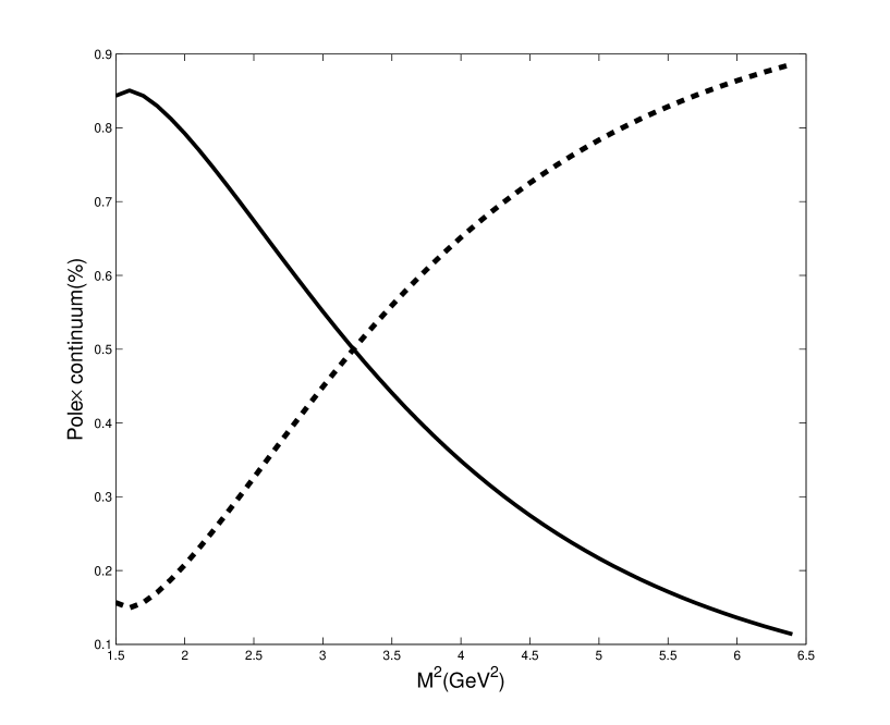
Figure 2: The solid line shows the relative pole contribution (the pole contribution divided by the total contribution) and the dashed line shows the relative continuum contribution for $\sqrt{s_{0}}=5.3~{}\mbox{GeV}$.

We fix the central value at the point $\sqrt{s_{0}}=5.3~{}\mbox{GeV}$. In Fig. 1 we plot contributions of all the terms in the OPE side of the sum rule. From this figure it can be seen that for $M^{2}\geq 2.5\,\mbox{GeV}^{2}$, the contribution of the dimension-6 condensate is less than 10% of the total contribution, which indicates a good Borel convergence. Therefore, we fix the lower value of $M^{2}$ in the sum rule window as $M^{2}_{min}=2.5$GeV².

Fig. 2 shows that the contributions from the pole terms and continuum terms with variation of the Borel parameter $M^{2}$. The pole contribution is bigger than the continuum contribution for $M^{2}\leq 3.3\,\mbox{GeV}^{2}$. Therefore, we fix $M^{2}_{max}=3.3\,\mbox{GeV}^{2}$ as the upper limit of the Borel window for $\sqrt{s_{0}}=5.3~{}\mbox{GeV}$. With the same analysis for the continuum threshold $\sqrt{s_{0}}=(5.3\pm 0.1)\mbox{GeV}$, we determine the corresponding Borel windows in Fig. 3. In this figure, we show the mass of X state as functions of the Borel mass for several threshold values $\sqrt{s_{0}}$. It can be seen that we get a very good Borel stability for $M_{x}$. It is worth noting that errors in our results merely come from the threshold $s_{0}$ and the Borel parameter $M^{2}$, without involving the ones from the variation of quark masses and QCD input parameters.

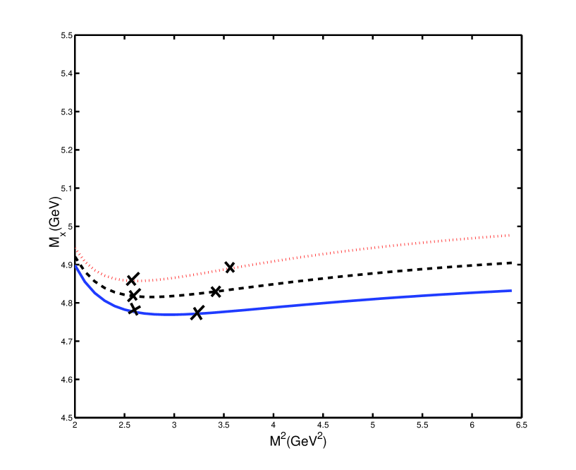
Figure 3: The X state mass, described with a $J^{PC}=1^{-+}$ tetraquark current, as a function of the sum rule parameter ($M^{2}$) for $\sqrt{s_{0}}=5.2$ GeV (solid line), $\sqrt{s_{0}}=5.3$ GeV (dotted line), and $\sqrt{s_{0}}=5.4$ GeV (dashed line). The crosses indicate the upper and lower limits in the Borel region.

Figure 4: The X state’s decay constant as a function of the sum rule parameter ($M^{2}$) for $\sqrt{s_{0}}=5.2$ GeV (solid line), $\sqrt{s_{0}}=5.3$ GeV (dotted line), and $\sqrt{s_{0}}=5.4$ GeV (dashed line). The crosses indicate the upper and lower limits in the Borel region.

Taking into account the uncertainties given above, we obtain the mass and decay constant of $X$

$$M_{x} = (4.82\pm 0.19)\,\rm{GeV}\,,$$

$$\lambda = (5.23\pm 0.28)\times 10^{-2}\,\rm{GeV^{5}}\,.$$ (10)

The mass obtained is not compatible with the mass of the narrow structure $X(4350)$ observed by Belle. It is, however, very interesting to notice that the mass obtained for a diquark-antidiquark state $c\bar{c}s\bar{s}$ with $J^{PC}=1^{--}$ is $m_{1^{--}}=(4.65\pm 0.10)~{}\mbox{GeV}$ Nielsen1 . It is smaller than what we have obtained with the $J^{PC}=1^{-+}$ tetraquark current. This may be an indication that it is easier to form tetraquark states with non-exotic quantum numbers. It is just as what the authors found in Ref. Nielsen that the mass of the molecular sate $D_{s}^{*+}\bar{D}_{s0}^{-}$ with $J^{PC}=1^{--}$ is lower than that with $J^{PC}=1^{-+}$. It is a hint that it is easier to form molecular sate states with non-exotic quantum numbers. We also notice that, Wang wang1 study $J^{P}=1^{-}$ tetraquark state whose interpolating current doesn’t have a definite charge conjugation using QCD sum rules, and obtained $m_{1^{-}}=(5.16\pm 0.16)\,\mbox{GeV}$. It is much larger than the results with a definite charge conjugation. Opposite to the $J^{P}=1^{-}$ $D_{s}^{*}D_{s0}^{*}$ molecular state circumstance, wherein, the state Zhang without a definite charge conjugation interpolator is much smaller than states with a definite charge conjugation interpolator Nielsen .

In summary, by assuming $X(4350)$ as a $[cs][\bar{c}\bar{s}]$ tetraquark state with quantum numbers $J^{PC}=1^{-+}$, the QCDSR approach has been applied to calculate the mass of the resonance. Our numerical result is $m_{X}=(4.82\pm 0.19)~{}\mbox{GeV}$, which disfavors the $X(4350)$ observed by the Belle is a $J^{PC}=1^{-+}$ tetraquark state.

References

(1)C. P. Shen et al., (Belle Collaboration), Phys.
Rev. Lett. 104, 112004 (2010).
(2)Z.-G. Wang, J. Phys. G 36, 085002 (2009).
(3) J. R. Zhang and M. Q. Huang, Commun. Theor. Phys. 54, 1075 (2010)
(4) F. Stancu, J. Phys. G. 37, 075017 (2010)
(5) Z.-G. Wang, Phys. Lett. B 690, 403 (2010).
(6) X. Liu, Z. G. Luo and Z. F. Sun, Phys. Rev. Lett. 104, 122001 (2010).
(7)R.M. Albuquerque, J.Dias and M. Nielsen, Phys. Lett. B 690, 141 (2010).
(8) Y.-L. Ma, Phys. Rev. D 82, 015013 (2010)
(9) M. A. Shifman, A. I. Vainshtein, and V. I. Zakharov, Nucl. Phys. B147, 385 (1979); B147, 448 (1979);
V. A. Novikov, M. A. Shifman, A. I. Vainshtein, and V. I. Zakharov, Fortschr. Phys. 32, 585 (1984), M. A. Shifman, Vacuum Structure and QCD Sum Rules, North-Holland, Amsterdam 1992.
(10)L. J. Reinders, H. R. Rubinstein, and S. Yazaki, Phys. Rep. 127, 1 (1985).
(11)P. Colangelo and A. Khodjamirian, in: M. Shifman (Ed.), At the Frontier of Particle
Physics: Handbook of QCD, vol. 3, Boris Ioffe Festschrift, World
Scientific, Sigapore, 2001, pp. 1495-1576, arXiv:0010175;
A. Khodjamirian, talk given at Continuous Advances in QCD
2002/ARKADYFEST, arXiv:0209166.
(12)M. Nielsen, F. S. Navarra, and S.H. Lee,
Phys. Rep. 497, 41 (2010).
(13)R. D. Matheus, S. Narison, M. Nielsen, and J. M. Richard, Phys. Rev. D 75, 014005 (2007);
S. H. Lee, K. Morita, and M. Nielsen, Phys.
Rev. D 78, 076001 (2008); M. E. Bracco, S. H. Lee, M. Nielsen,
R. R. daSilva, Phys. Lett. B 671, 240 (2009); S. H. Lee,
K. Morita, and M. Nielsen, Nucl. Phys. A 815, 29 (2009);
R. M. Albuquerque and M. Nielsen, Nucl. Phys. A 815, 53 (2009).
(14)C. Y. Cui, Y. L. Liu, M. Q. Huang, Phys. Rev. D 85, 074014 (2012); C. Y. Cui, Y. L. Liu, G. B. Zhang, M. Q. Huang, Commun. Theor. Phys. 57 (2012) 1033-1036; C. Y. Cui, Y. L. Liu, W. B. Chen, M. Q. Huang, arXiv:1304.1850 [hep-ph]; C. Y. Cui, Y. L. Liu, M. Q. Huang, arXiv:1308.3625 [hep-ph]; J. R. Zhang and M. Q. Huang, Phys. Rev. D 77, 094002 (2008); Phys. Rev. D 78, 094007 (2008); Phys. Lett. B 674, 28 (2009); J. Phys. G 37, 025005 (2010).
(15)S. Narison, QCD Spectral Sum Rules, World Scientific,Singapore,1989.