A long-lived Higgs mode in a two-dimensional confined Fermi gas

Abstract

The Higgs mode corresponds to the collective motion of particles due to the vibrations of an invisible field. It plays a fundamental role for our understanding of both low and high energy physics, giving elementary particles their mass and leading to collective modes in condensed matter and nuclear systems. The Higgs mode has been observed in a limited number of table-top systems, where it however is characterised by a short lifetime due to decay into a continuum of modes. A major goal which has remained elusive so far, is therefore to realise a long-lived Higgs mode in a controllable system. Here, we show how an undamped Higgs mode can be observed unambiguously in a Fermi gas in a two-dimensional trap, close to a quantum phase transition between a normal and a superfluid phase. We develop a first-principles theory of the pairing and the associated collective modes, which is quantitatively reliable when the pairing energy is much smaller than the trap level spacing, yet simple enough to allow the derivation of analytical results. The theory includes the trapping potential exactly, which is demonstrated to stabilize the Higgs mode by making its decay channels discrete. Our results show how atoms in micro-traps can unravel properties of a long-lived Higgs mode, including the role of confinement and finite size effects.

According to the standard description of many-body systems, the broken symmetry state of a system is characterised by a collective field. Phase oscillations of this field gives rise to massless Goldstone modes, whereas oscillations in the amplitude correspond to the massive Higgs mode Anderson1958 ; Bogoliubov1958 ; Higgs1964 . The Higgs mode plays a fundamental role in our understanding of nature across many energy scales: It leads to the existence of collective modes in condensed matter systems Sachdev2011book , pair vibration modes in atomic nuclei BohrMottelson1975book ; Potel2013 , and in the Standard Model it gives elementary particles their mass  Higgs1964 , as was recently confirmed in two spectacular experiments at CERN CMS2012 ; ATLAS2012 . It is therefore desirable to have controllable table-top systems where one can investigate fundamental questions such as the existence of a sharp Higgs mode which is stable against decay Podolsky2011 , and the interplay between confinement and the Higgs mode, which is relevant for atomic nuclei as well as particle physics models with compact dimensions Randall1999 ; Arkani-Hamed1998 . Also, since the Higgs mode is a consequence of the broken symmetry of a many-particle state, an intriguing question is to examine how this mode emerges with increasing particle number. The list of table-top systems where the Higgs mode has been observed is fairly short. Raman scattering data for a niobium selenide superconductor are consistent with a Higgs mode coupled to a charge-density wave Measson2014 ; Littlewood1981 ; Sooryakumar1980 . Also, the Higgs mode has been identified in neutron scattering experiments for a quantum anti-ferromagnet Ruegg2008 , and in lattice modulation experiments for a gas of bosonic atoms in an optical lattice Endres2012 ; Bissbort2011 . In these cases, the spectral signal of the Higgs mode is however very broad due to decay into a continuum of modes which complicates a quantitative analysis.

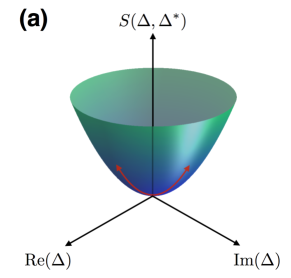
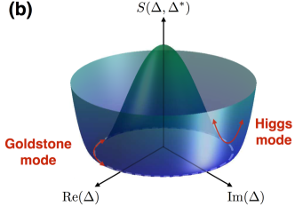
Figure 1: The free energy of the system as a function of the pairing field and the associated Higgs and Goldstone modes. (a) the weak coupling regime where the system is in the normal phase ($\epsilon_{B}<\epsilon_{B}^{c}$). (b) the strong coupling superfluid regime ($\epsilon_{B}>\epsilon_{B}^{c}$). The Higgs mode corresponds to amplitude fluctuations around the minimum of the effective action. At the quantum phase transition point between the two phases, $\epsilon_{B}=\epsilon_{B}^{c}$, the Gaussian amplitude fluctuations around $\Delta=0$ cost zero energy. The Goldstone mode corresponds to phase fluctuations in the superfluid phase.

Here, we develop a microscopic theory for the pairing of a gas of fermionic atoms confined in a two-dimensional (2D) harmonic trap. The theory includes the trapping potential exactly, and it is quantitatively reliable in the regime where the pairing energy is smaller than the trap level spacing. We derive several analytical results for the pairing properties and the associated Higgs and Goldstone modes. In particular, we demonstrate that for certain ”magic numbers” of particles trapped, a sharp Higgs mode appears close to a quantum phase transition between the normal and a superfluid phase. The trapping potential is shown to stabilise the Higgs mode against decay, since the level spacing of the Goldstone spectrum is larger than the mode frequency close to the phase transition. We demonstrate how the Higgs mode can be excited and investigated systematically in a new generation of experiments confining atoms in micro-traps, which are well suited to form 2D systems.

I The system

We consider a 2D system of fermionic atoms of mass $m$ with an equal number in two internal states denoted spin $\sigma=\uparrow,\downarrow$. The particles are trapped in a circular symmetric potential $V(r)=m\omega_{\perp}^{2}r^{2}/2$ where $r^{2}=x^{2}+y^{2}$ and the temperature $T$ is zero. The 2D confinement can be realised by a tight trapping potential $m\omega_{z}^{2}z^{2}/2$ in the $z$-direction Martiyanov2010 ; Feld2011 ; Sommer2012 ; Zhang2012 with $\omega_{z}$ larger than any other relevant energy. For low densities, only the short range $s$-wave interaction between particles with opposite spin is important, and it can be modelled by a contact interaction $g\delta({\mathbf{r}})$ with a high energy cut-off, where $\delta({\mathbf{r}})$ is the 2D delta function. When the 3D scattering length $a$ is much smaller than $l_{z}=1/\sqrt{m\omega_{z}}$, $g$ can be obtained by integrating the 3D pseudopotential over the oscillator ground state in the $z$-direction yielding $g=\sqrt{2\pi}a/ml_{z}$. Here, we will eliminate $g$ in favor of the two-body binding energy to obtain results independent of the cut-off.

We focus on the pairing properties of this system using a functional approach, which highlights the collective modes connected with pairing oscillations in a particularly lucid way. Performing a Hubbard-Stratonovich transformation to introduce the pairing field $\Delta(x)$, the partition function of the system can be written as $\mathcal{Z}=\int{\mathcal{D}}(\Delta\Delta^{*})\exp[-S(\Delta,\Delta^{*})]$ with the action

$$S(\Delta,\Delta^{*})=-\rm{Tr}\log{\mathcal{G}}^{-1}-\frac{1}{g}\int_{0}^{\beta}d\tau\int d^{2}r|\Delta(x)|^{2}.$$ (1)

Here $x=({\mathbf{r}},\tau)$ with $\tau$ the imaginary time, and the inverse Green’s function is

$${\mathcal{G}}^{-1}(x,x^{\prime})=\begin{bmatrix}\partial_{\tau}+H_{0}&-\Delta(x)\\ -\Delta(x)^{*}&\partial_{\tau}-H_{0}\end{bmatrix}\delta(x-x^{\prime})$$ (2)

with $H_{0}=-\nabla^{2}/2m+V(r)-\epsilon_{F}$ the single particle Hamiltonian minus the Fermi energy $\epsilon_{F}$ (We take $\hbar=1$). The trace in (1) is over $x$ and spin space. We ignore the mean-field (Hartree) correction to the single particle energy since the density and therefore the Hartree potential is harmonic in the Thomas-Fermi approximation for a 2D gas. Consequently, it can be included simply by renormalising the trapping frequency $\omega_{\perp}$. Figure 1 illustrates the action $S(\Delta,\Delta^{*})$ in the normal and superfluid phases, and the corresponding Goldstone and Higgs modes.

II Pairing and single particle properties

The instability towards pairing is described using mean-field theory, which is obtained as usual from the stationary phase approximation to ${\mathcal{Z}}$ yielding the Bogoliubov-de Gennes (BdG) equations deGennes1989book . We expand the corresponding Bogoliubov wave-functions in the eigenfunctions $\phi_{nm}({\mathbf{r}})$ of the single particle Hamiltonian, i.e. $H_{0}\phi_{nm}({\mathbf{r}})=\xi_{n}\phi_{nm}({\mathbf{r}})$ with $\xi_{n}=(n+1)\omega_{\perp}-\epsilon_{F}$, $\phi_{nm}({\mathbf{r}})=R_{nm}(r)\exp(im\phi)/\sqrt{2\pi}$, and $m=-n,-n+2,\ldots n$ the angular momentum along the $z$-axis. The ground state is circular symmetric corresponding to pairing between $\uparrow$ and $\downarrow$ atoms with opposite angular momentum. The pairing between particles in shells $n$ and $n^{\prime}$ is given by the matrix element (see Appendix A)

$$\Delta_{nn^{\prime}m}=\int_{0}^{\infty}drrR_{nm}(r)R_{n^{\prime}m}(r)\Delta(r)$$ (3)

with $\Delta({\mathbf{r}})=g\langle\psi_{\downarrow}({\mathbf{r}})\psi_{\uparrow}({\mathbf{r}})\rangle$ the mean-field pairing field. Here, $\psi_{\sigma}({\mathbf{r}})$ is the field operator annihilating a particle with spin $\sigma$ at position ${\mathbf{r}}$. Since $\Delta(r)$ has a definite sign in the ground state whereas the sign of the radial functions $R_{nm}(r)$ in general oscillates, the intershell matrix elements with $n^{\prime}\neq n$ are suppressed compared to the intrashell matrix elements with $n^{\prime}=n$ in (3). We can therefore ignore the intershell matrix elements when the pairing energy is small compared to the trap level spacing $\omega_{\perp}$, i.e. $\Delta_{nn^{\prime}m}\ll\omega_{\perp}$. We refer to this regime as intrashell pairing, since the Cooper pairs are formed within each harmonic oscillator shell. The BdG equations then simplify into $2\times 2$ matrix equations for each pair of quantum numbers $(n,m)$, with the solutions $E_{nm}=(\xi_{n}^{2}+\Delta_{nnm}^{2})^{1/2}$, $u_{nm}^{2}=(1+\xi_{n}/E_{nm})/2$, and $v_{nm}^{2}=(1-\xi_{n}/E_{nm})/2$. In addition, the $m$-dependence of $\Delta_{nnm}$ is weak which can be shown explicitly using the Thomas-Fermi approximation (see Appendix A). We therefore make the approximation $\Delta_{nnm}\simeq\Delta_{n}\equiv\sum_{m=-n}^{n}\Delta_{nnm}/\Omega_{n}$, where $\Omega_{n}=n+1$ is the degeneracy of the $n$’th shell. Using that the main contribution to the pairing is from the shells around the Fermi level, we end up with the gap equation (see Appendix A)

$$-\frac{1}{G}=\sum_{n}\frac{1}{2E_{n}}=\sum_{n}\frac{1}{2\epsilon_{n}-\epsilon_{\rm tb}}$$ (4)

where $E_{n}=(\xi_{n}^{2}+\Delta_{n}^{2})^{1/2}$ with $\Delta_{n}=\Delta/\sqrt{\Omega_{n}}$, and $\epsilon_{n}=(n+1)\omega_{\perp}$. The effective coupling strength is

$$G=2\pi g\frac{\int_{0}^{\infty}drr\rho_{n_{F}}(r)^{2}}{\Omega_{n_{F}}},$$ (5)

where $n_{F}$ denotes the highest occupied shell in the normal phase, and $\rho_{n}(r)=\sum_{m}R_{nm}(r)^{2}/2\pi$ is the particle density of a completely filled shell $n$.

In the second equality in (4), we have used that the energy $\epsilon_{\rm tb}$ of a two-body state is determined by $1/G=-\sum_{n}1/({2\epsilon_{n}-\epsilon_{\rm tb}})$ as explained in Appendix B. In the perturbative regime, this yields $\epsilon_{\rm tb}=2\epsilon_{n}+G=2\epsilon_{n}+\sqrt{2}a\omega_{\perp}/\sqrt{\pi}l_{z}$, where we have used the Thomas-Fermi result $G=g/2\pi l^{2}$ and $g=\sqrt{2\pi}a/ml_{z}$ for weak confinement $a\ll l_{z}$ (see Appendix A). This recovers the exact result for the two-body binding energy of an $s$-wave state in a 2D Harmonic trap in the perturbative regime Busch1998 , which illustrates an important point: The approximations we make are systematic, and (4) is it not merely a schematic model – it provides an accurate description of the correlations with monopole symmetry in the instrashell regime. By replacing $1/G$ by the two-body energy, we have arrived at quantitative reliable theory for the monopole pairing correlations, which is well-defined for an infinite cut-off. It represents a crucial simplification which allows us to derive several analytical results. For a 3D spherical trap, similar approximations were shown to yield very accurate results when compared to a full solution of the BdG equations Bruun2002a .

There are two qualitatively different cases for pairing: The open shell case $\epsilon_{F}=(n_{F}+1)\omega_{\perp}$ where the highest occupied shell $n=n_{F}$ is partly filled, and the ”magic number” case $\epsilon_{F}=(n_{F}+3/2)\omega_{\perp}$ with a completely filled highest shell $n=n_{F}$. We parametrise the interaction strength by the two-body binding energy $\epsilon_{B}>0$ per particle, defined as $\epsilon_{\rm tb}=2\omega-2\epsilon_{B}$. To obtain analytical results, we expand (4) in $\Delta/\omega_{\perp}$ and $\epsilon_{B}/\omega_{\perp}$. For the open shell case, this yields after evaluating the sums

$$\Delta_{n_{F}}=\frac{\epsilon_{B}}{1-\epsilon_{B}(\gamma+\ln n_{F})/\omega_{\perp}},$$ (6)

where $\gamma=0.577$ is the Euler-Mascheroni constant and we have ignored $1/n_{F}$ corrections.

For the closed shell case $\epsilon_{F}=(n_{F}+3/2)\omega_{\perp}$, there is only pairing for strong enough attraction when it is energetically favourable to excite pairs from the highest filled shell $n=n_{F}$ to the lowest empty shell $n=n_{F}+1$ as illustrated in Fig. 2. Expanding (4) in $\Delta/\omega_{\perp}$ and $\epsilon_{B}/\omega_{\perp}$ yields

$$\frac{\epsilon^{c}_{B}}{\omega_{\perp}}=\frac{B(n_{F})}{2\xi(2)}[\sqrt{1+4\xi(2)/B(n_{F})^{2}}-1]$$ (7)

for the critical attraction strength for pairing with $B(n_{F})=\gamma+4\ln 2+\ln n_{F}$ and $\xi(z)$ Riemann’s zeta function. For $\epsilon_{B}>\epsilon_{B}^{c}$, we obtain

$$\Delta_{n_{F}}=\frac{\omega_{\perp}}{\sqrt{7\xi(3)}}\sqrt{\frac{\omega_{\perp}}{\epsilon^{c}_{B}}-\frac{\omega_{\perp}}{\epsilon_{B}}+\xi(2)\left(\frac{\epsilon_{B}}{\omega_{\perp}}-\frac{\epsilon^{c}_{B}}{\omega_{\perp}}\right)}$$ (8)

for the pairing energy.

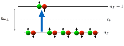
Figure 2: For the closed shell case, there is only pairing for strong enough attraction, $\epsilon_{B}>\epsilon_{B}^{c}$, so that is is energetically favourable to excite Cooper pairs from the highest occupied to the lowest empty shell. The collective mode in the normal phase is formed by making coherent excitations pairs across the chemical, and the mode frequency goes to zero when the system becomes unstable to pairing.

III Collective modes

We now analyse the collective modes arising from the fluctuations $\delta\Delta(x)$ of the pairing field around the mean-field solution. These fluctuations are included by writing $\mathcal{G}^{-1}=\mathcal{G}_{\rm mf}^{-1}-\Sigma$ where $\mathcal{G}^{-1}_{\rm mf}$ is given by (2) using the mean-field pairing field, and

$$\Sigma(x)=\begin{bmatrix}0&\delta\Delta(x)\\ \delta\Delta(x)^{*}&0\end{bmatrix}$$ (9)

contains the fluctuations. We have $\rm{Tr}\log\mathcal{G}^{-1}=\rm{Tr}\log\mathcal{G}_{\rm mf}^{-1}-\sum_{n=1}^{\infty}\rm{Tr}[(\mathcal{G}_{\rm mf}\Sigma)^{n}]/n$, and since the linear term vanishes as we expand around a stationary point, we obtain $S(\Delta,\Delta^{*})\simeq-\rm{Tr}\log\mathcal{G}_{\rm mf}^{-1}+S_{2}(\delta\Delta,\delta\Delta^{*})$ to quadratic order. Here $S_{2}(\delta\Delta,\delta\Delta^{*})={\rm Tr[\mathcal{G}_{\rm mf}\Sigma\mathcal{G}_{\rm mf}\Sigma]}/2-\int d^{3}r|\delta\Delta(x)|^{2}/g$. As explained in Appendix C, evaluating the trace and the resulting Matsubara sums yields $S_{2}=T\sum_{l}[s_{2}(i\omega_{l})-\int d^{2}r\mathbf{d}({\mathbf{r}},i\omega_{l})^{\dagger}\mathbf{d}({\mathbf{r}},i\omega_{l})/g]/2$ with $\mathbf{d}({\mathbf{r}},i\omega_{l})^{\dagger}=[\delta\Delta({\mathbf{r}},i\omega_{l})^{*},\delta\Delta({\mathbf{r}},-i\omega_{l})]$ and $\omega_{l}=2l\pi T$ with $l=0,\pm 1,\pm 2\ldots$ a Bose Matsubara frequency.

To find the collective modes, we analytically continue to real time $i\omega_{l}\rightarrow\omega+i0_{+}$. The collective mode frequencies $\omega$ are then obtained by finding the zeroes in the inverse pair fluctuation propagator $s_{2}(\omega)$. For low energy, the collective modes split into phase and amplitude fluctuations, and we therefore write $\delta\Delta({\mathbf{r}},t)=[\kappa({\mathbf{r}},t)+i\theta({\mathbf{r}},t)]/\sqrt{2}$ where $t$ is time Engelbrecht1997 . Both $\kappa({\mathbf{r}},t)$ and $\theta({\mathbf{r}},t)$ are real and they describe amplitude (Higgs) and phase (Goldstone) fluctuations respectively. We find

$$s_{2}(\omega)=\int d^{2}rd^{2}r^{\prime}\mathbf{v}({\mathbf{r}},\omega)^{\dagger}{\mathbf{A}}({\mathbf{r}},{\mathbf{r}}^{\prime},\omega)\mathbf{v}({\mathbf{r}}^{\prime},\omega)$$ (10)

where ${\mathbf{A}}({\mathbf{r}},{\mathbf{r}}^{\prime},\omega)=\sum_{nm}|\phi_{nm}({\mathbf{r}})|^{2}{\mathbf{A}}(n,\omega)|\phi_{nm}^{*}({\mathbf{r}}^{\prime})|^{2}$,

$$A_{11}(n,\omega)=\frac{\xi_{n}^{2}}{2E_{n}(\omega^{2}-4E_{n}^{2})}\hskip 14.22636ptA_{22}(n,\omega)=\frac{2E_{n}}{\omega^{2}-4E_{n}^{2}}$$

$$A_{12}(n,\omega)=-A_{21}(n,\omega)=i\omega\frac{u_{n}^{4}-v_{n}^{4}}{4E_{n}^{2}-\omega^{2}},$$ (11)

and ${\mathbf{v}}({\mathbf{r}},\omega)^{\dagger}=[\kappa({\mathbf{r}},\omega)^{*},\theta({\mathbf{r}},\omega)^{*}]$.

III.1 The Goldstone mode

The Goldstone mode is found by solving $\int d^{2}r^{\prime}{\mathbf{A}}_{22}({\mathbf{r}},{\mathbf{r}}^{\prime},\omega)\theta({\mathbf{r}}^{\prime})=\theta({\mathbf{r}})/g$. We take a circular symmetric eigenfunction $\theta(r)$ corresponding to a monopole mode. In the spirit of the intra-shell regime, we ignore the weak $n,m$-dependence of the resulting integrals, when ${\mathbf{A}}({\mathbf{r}},{\mathbf{r}}^{\prime},\omega)$ is expressed in terms of the functions $\phi_{nm}({\mathbf{r}})$. As detailed in Appendix C, this gives the eigenvalue equation

$$\sum_{n}\frac{2E_{n}}{4E_{n}^{2}-\omega^{2}}=\sum_{n}\frac{1}{2\epsilon_{n}-\epsilon_{\rm tb}}$$ (12)

for the collective Goldstone mode, where we again have used the two-body energy to eliminate the coupling constant $G$. Using the gap equation (4), we see that $\omega=0$ is a solution to (12). Since $A_{12}({\mathbf{r}},{\mathbf{r}}^{\prime},\omega)\propto\omega$ and $A_{21}({\mathbf{r}},{\mathbf{r}}^{\prime},\omega)\propto\omega$, this solution is furthermore completely decoupled from the amplitude oscillations. The theory thus recovers the zero energy Goldstone mode corresponding to the broken $U(1)$ symmetry of the phase of the pairing field.

III.2 The Higgs mode

The Higgs amplitude mode is found by solving $\int d^{2}r^{\prime}{\mathbf{A}}_{11}({\mathbf{r}},{\mathbf{r}}^{\prime},\omega)\kappa({\mathbf{r}}^{\prime})=\kappa({\mathbf{r}})/g$. Taking $\kappa({\mathbf{r}})$ to be circular symmetric and ignoring again the weak $n,m$ dependence of the integrals yields an eigenfuction of the form $\kappa({\mathbf{r}})\propto\sum_{n}A_{11}(n,\omega)\rho_{n}({\mathbf{r}})$. We obtain (see Appendix C)

$$\sum_{n}\frac{2\xi_{n}^{2}}{E_{n}(4E_{n}^{2}-\omega^{2})}=\sum_{n}\frac{1}{2\epsilon_{n}-\epsilon_{\rm tb}}.$$ (13)

Assuming perfect particle-hole symmetry around the Fermi level, we see from the gap equation (4) that $\omega=2\Delta_{n_{F}}$ is a solution. This mode is decoupled from the Goldstone modes and therefore undamped, since it follows from (11) that $\sum_{n}{\mathbf{A}}_{12}(n,2\Delta_{n_{F}})=\sum_{n}{\mathbf{A}}_{21}(n,2\Delta_{n_{F}})=0$ for perfect particle-hole symmetry. This is the undamped Higgs mode for the superfluid phase corresponding to monopole amplitude oscillations of the pairing field. Note that particle-hole symmetry is equivalent to a Lorentz-invariant low energy effective theory Varma2002 .

Including the particle-hole asymmetry around the Fermi level changes the mode frequency only by a small amount when $n_{F}$ is not too small, as will be confirmed numerically below. In addition, it leads to damping of the Higgs mode due to coupling to the Goldstone modes. This damping is however weak for two reasons. First, in the intrashell regime pairing mainly occurs in the shells around the Fermi energy which are approximately particle-hole symmetric leading to a weak coupling to the Goldstone modes. Second, the Goldstone modes correspond to density oscillations with a typical energy $\sim\omega_{\perp}$ both in the collisionless and in the hydrodynamic regimes Pitaevskii1997 ; Gao2012 ; Baur2013 . The Higgs mode is therefore well separated in energy from these modes since $\Delta\ll\omega_{\perp}$ in the intrashell regime. In the open shell case, there are however low lying pair breaking excitations with energy $\sim 2\Delta$ which can damp the Higgs mode, but in the closed shell case, no such low energy modes exist since the lowest single particle energies are $(\omega_{\perp}^{2}/4+\Delta_{n_{F}}^{2})^{1/2}$. The existence of a well defined Higgs mode with a sharp spectral peak for the closed shell case is one of the main results of this paper. The lack of damping of this mode is a major advantage compared to previous experimental table-top realisations of the Higgs mode, where coupling to a continuum of modes leads to significant damping Podolsky2011 ; Endres2012 .

III.3 Normal phase

In the closed shell case, the system is in the normal phase for weak attraction with $\epsilon_{B}<\epsilon_{B}^{c}$. In this case, (13) has to be solved with $E_{n}=|\xi_{n}|$ and the amplitude modes correspond to coherently either adding a pair of particles, or removing a pair of particles. The particle conserving collective modes correspond to subsequently adding and removing a pair of particles, and their frequencies is therefore twice the frequency obtained by solving (13). In the weak coupling regime $\epsilon_{B}\ll\epsilon_{B}^{c}$, we obtain the collective mode frequency $\omega=2\omega_{\perp}-4\epsilon_{B}$. This result can also be derived directly from first order perturbation theory using $|E\rangle=\Gamma_{n_{F}+1}^{\dagger}\Gamma_{n_{F}}|G\rangle$ for the excited state, where $\Gamma_{n}^{\dagger}=\sum_{m}a_{nm\uparrow}^{\dagger}a_{n-m\downarrow}^{\dagger}/\sqrt{\Omega_{n}}$ and $|G\rangle$ is the non-interacting ground state with all shells up to and including $n_{F}$ completely filled. The state $|E\rangle$ is formed by exciting $\uparrow\downarrow$ pairs of from the highest fully occupied shell $n_{F}$ to the lowest unoccupied shell $n_{F}+1$. The excitation energy initially decreases with increasing attraction since the particles can increase their overlap in the excited state. When the excitation energy goes to zero, the system can spontaneously excite pairs from the shell $n_{F}$ to the shell $n_{F}+1$, and it is unstable towards Cooper pair formation, see Fig. 2. Close to critical coupling strength for pairing $\epsilon_{B}\lesssim\epsilon_{B}^{c}$, we expand (13) in $\epsilon_{B}/\omega_{\perp}$ and $\omega/\omega_{\perp}$. Evaluating the resulting sums to accuracy $1/n_{F}$ yields

$$\frac{\omega}{\omega_{\perp}}=\frac{2}{\sqrt{7\xi(3)}}\sqrt{\frac{\omega_{\perp}}{\epsilon_{B}}-\frac{\omega_{\perp}}{\epsilon^{c}_{B}}+\xi(2)\left(\frac{\epsilon^{c}_{B}}{\omega_{\perp}}-\frac{\epsilon_{B}}{\omega_{\perp}}\right)}.$$ (14)

IV Numerical results

The Higgs mode frequency obtained from (13) with $n_{F}=10$ is shown in Fig. 3 for the open shell case. We see that there is very good agreement between the numerical solution and the analytical results. The numerical solution of (13) is essentially indistinguishable from $2\Delta_{n_{F}}$ with $\Delta_{n_{F}}$ determined from (6). This agreement shows that particle-hole asymmetry has a negligible effect on the collective mode frequency as well as on the single particle pairing, so that that (6) is an accurate expression for the solution to the gap equation (4). The pairing and therefore the Higgs mode energy grows linearly with the binding energy for weak coupling whereas it increases more quickly when more shells participate in the pairing. In the case of smaller particle numbers, i.e. smaller $n_{F}$, the analytical results agrees less with the numerics, since particle-hole asymmetry ($1/n_{F}$ effects) become larger.

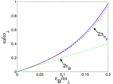
Figure 3: The Higgs mode for the open shell case. We plot the Higgs amplitude mode energy as a function of the two-body binding energy per particle $\epsilon_{B}$ for the open shell case with $n_{F}=10$. The solid line is obtained by numerically solving (13), the dashed line is $\omega=2\Delta_{n_{F}}$ with $\Delta_{n_{F}}$ given by (6), and the dotted line is $\omega=2\epsilon_{B}$.

In Fig. 4, we plot the Higgs mode frequency for the closed shell case with $n_{F}=10$. Again, we see that the analytical formulas agree very well with the numerical solution showing that particle-hole asymmetry has a negligible effect on pairing and the Higgs mode frequency in the intrashell regime. As for the open shell case, the agreement is less for smaller $n_{F}$. The energy initially decreases from non-interacting value $2\omega_{\perp}$ with increasing binding $\epsilon_{B}$. At the critical coupling strength for pairing, the mode has zero frequency and for stronger attraction when the system is superfluid, the frequency is $2\Delta_{n_{F}}$. This characteristic non-monotonic behaviour of the Higgs frequency near the quantum phase transition has a clear interpretation in terms of the effective interaction and broken symmetry (see Fig. 1), and it provides a smoking gun signal for the Higgs mode.

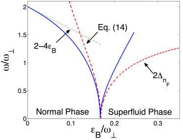
Figure 4: The Higgs mode for the closed shell case. We plot the Higgs amplitude mode energy as a function of the two-body binding energy per particle $\epsilon_{B}$ for the closed shell case with $n_{F}=10$. The solid line is obtained by numerically solving (13), and the dashed lines are (14) for $\epsilon_{B}<\epsilon_{B}^{c}$, and $\omega=2\Delta_{n_{F}}$ with $\Delta_{n_{F}}$given by (8) for $\epsilon_{B}>\epsilon_{B}^{c}$. The critical two-body binding energy $\epsilon_{B}^{c}$ is given by (7). The dotted line is the perturbative result $\omega=2\omega_{\perp}-4\epsilon_{B}$.

We note that the intrashell ansatz eventually breaks down when $\Delta_{n_{F}}$ is comparable to $\omega_{\perp}$ and matrix elements with $n^{\prime}\neq n$ in (3) become important. This corresponds to the coherence length of the Cooper pairs becoming smaller than the system size. The system then approaches the bulk limit where the Higgs mode becomes damped by coupling to the Goldstone modes. In the case of a 3D harmonic trap, a comparison with a full solution to the BdG equations shows that the breakdown of the intrashell regime occurs for $\Delta_{N}\simeq\omega_{\perp}/2$ both at the single particle level Bruun2002a , and for the collective modes Bruun2002b ; Bruun2001 .

V Experimental realisation

The Higgs amplitude mode does not couple strongly to density oscillations which makes it hard to observe in condensed matter systems Varma2002 . For cold atoms it can on the other hand be excited rather straightforwardly by modulating the coupling strength between the atoms for instance by changing the external magnetic field close to a Feshbach resonance. This leads to a time-dependent interaction of the form $H_{\rm int}=G(t)\sum_{nn^{\prime}}\Gamma_{n}^{\dagger}\Gamma_{n^{\prime}}$, which couples strongly to the Higgs mode by exciting pairs across the Fermi energy, see Fig. 2 and Appendix B. When $G(t)$ is modulated at the resonance frequency, the Higgs mode will be excited which can be detected for instance by measuring the energy transferred to the system. For a small system, the transferred energy should be sizable fraction of the total energy. Alternatively, the Higgs mode could be detected by counting the number of atoms excited to higher shells. The number of atoms in individual oscillator levels was recently counted with single atom precision using a new generation of micro traps Serwane2011 ; Zurn2012 . The trapping frequencies are of the order $\sim 10$kHz in these experiments, which means that for $T\ll 500$nK, effects of a non-zero temperature are small and one should be able to observe the effects described in this paper. Finally, while present micro traps realise 1D systems with less than 10 particles, it is experimentally feasible to make these systems 2D, which in addition could increase the particle number WeitenbergJochim2014 .

A small particle number will give rise to significant finite size effects such as the lack of a sharp quantum phase transition where the Higgs mode frequency goes to zero. Instead, the finite size version of the Higgs mode will be characterised by a smooth non-monotonic frequency as a function of the attraction: First, it will decrease with increasing attraction until it reaches a differentiable minimum of non-zero frequency, after which it increases with increasing attraction. The minimum frequency will decrease with increasing particle number becoming sharper and sharper at the same time, as the system approaches the many-body limit. This transition between few- and many-body dynamics will be very interesting to observe.

VI Conclusions and outlook

We developed a microscopic theory for pairing and collective modes in a trapped 2D Fermi gas, which takes the trapping potential into account exactly. The theory is quantitatively reliable when the pairing energy is much smaller than the trap level spacing, and at the same it is simple enough to allow the derivation of several analytical results. Using this theory, we demonstrated the existence of a sharp Higgs mode close to the quantum phase transition between a normal and a superfluid phase, when the system is in a closed shell configuration. The trapping confinement was shown to stabilise the Higgs mode against decay, since it makes the Goldstone spectrum discrete with a level spacing much larger than the Higgs energy. We then discussed how a new generation of cold atom experiments using micro traps can realise the physics described in this paper.

Our results open up the intriguing prospect of using cold atoms in micro traps to observe for the first time a long lived Higgs mode in a confined geometry. This is relevant to certain models in high energy physics Randall1999 ; Arkani-Hamed1998 , as well as to the so-called pair vibration modes, which play a central role in the theory of atomic nuclei BohrMottelson1975book ; Potel2013 . In atomic nuclei, it is however very challenging to calculate the properties of these modes microscopically, and they are furthermore probed rather indirectly in nucleon transfer reactions whose interpretation is subject to intense debate. Finally, we discussed how micro traps can be used to investigate the fundamental question how the ”standard model” of broken symmetry and collective modes in condensed matter physics emerges, as the dynamics changes from few- to many-body physics with increasing particle number Sachdev2011book ; Wenz2013 .

Appendix A The Bogoliubov-de Gennes equations

We expand the Bogoliubov wave-functions $[u_{m}^{\eta}({\mathbf{r}}),v_{m}^{\eta}({\mathbf{r}})]$ in the eigenfunctions of the single particle Hamiltonian, i.e. $u^{\eta}_{m}({\mathbf{r}})=\sum_{n}u^{\eta}_{nm}\phi_{nm}({\mathbf{r}})$ and likewise for $v^{\eta}_{m}({\mathbf{r}})$. In this basis, the Bogoliubov-de Gennes equations read

$$E^{\eta}_{m}\begin{bmatrix}u^{\eta}_{nm}\\ v^{\eta}_{nm}\end{bmatrix}=\sum_{n^{\prime}}\begin{bmatrix}\xi_{n}\delta_{n,n^{\prime}}&\Delta_{nn^{\prime}m}\\ \ \Delta_{nn^{\prime}m}&-\xi_{n}\delta_{n,n^{\prime}}\end{bmatrix}\begin{bmatrix}u^{\eta}_{n^{\prime}m}\\ v^{\eta}_{n^{\prime}m}\end{bmatrix}$$ (15)

for the quasiparticle energies $E_{m}^{\eta}$. The pairing matrix element is given by (3). Since the $m$-dependence is weak, we make the approximation $\Delta_{nnm}\simeq\Delta_{n}\equiv\sum_{m=-n}^{n}\Delta_{nnm}/\Omega_{n}$, and the self-consistent gap equation (3) becomes

$$\Delta_{n}=-g\sum_{n^{\prime}}\frac{\Delta_{n^{\prime}}}{2E_{n^{\prime}}}\frac{\int_{0}^{\infty}drr\rho_{n}(r)\rho_{n^{\prime}}(r)}{\int_{0}^{\infty}drr\rho_{n}(r)}$$ (16)

where we have used $\Omega_{n}=\sum_{m}\int_{0}^{\infty}drrR_{nm}(r)^{2}$. From (16), we can define an appropriately symmetrized effective coupling strength between the shells $n$ and $n^{\prime}$ as

$$G_{nn^{\prime}}=2\pi g\frac{\int_{0}^{\infty}drr\rho_{n}(r)\rho_{n^{\prime}}(r)}{\sqrt{\Omega_{n}\Omega_{n^{\prime}}}}.$$ (17)

The effective coupling strength depends only weakly on $n$ and $n^{\prime}$ for the shells around the Fermi energy which contribute most to the pairing. We therefore write $G_{nn^{\prime}}\simeq G_{n_{F}n_{F}}\equiv G$, and the gap equation (16) simplifies to (4). The pairing field corresponding to this solution is

$$\Delta(r)=-g\sum_{n}\frac{\Delta_{n}}{2E_{n}}\rho_{n}(r).$$ (18)

The weak $m$-dependence of the pairing can be checked by invoking the Thomas-Fermi approximation. In the Thomas-Fermi regime $n\gg 1$, we have $\rho_{n}(r)=\partial_{n}\rho(r)=1/2\pi l^{2}$ for $r<\sqrt{2n+1}l$ and $\rho_{n}(r)=0$ for $r>\sqrt{2n+1}l$ with $l=1/\sqrt{m\omega_{\perp}}$. Here, $\partial_{n}\rho(r)$ is the derivative of the total (single spin) density $\rho(r)$ of filled shells up to and including $n$, with respect to $n$. We have $\rho(r)=(n_{F}+1)(1-r^{2}/R_{TF}^{2})/2\pi l^{2}$ for a 2D gas at $T=0$ with $T_{TF}=\sqrt{2n_{F}+1}l$. Using this in (5), we obtain $G=g/2\pi l^{2}$ in the Thomas-Fermi regime. For weak coupling, when only the highest occupied shell $n=n_{F}$ contributes to the pairing we then obtain from (18) $\Delta(r)=-g/4\pi l^{2}$ for $r<R_{TF}$, i.e. $\Delta(r)$ is simply a constant. It follows that $\Delta_{nnm}=\int_{0}^{\infty}drrR_{nm}(r)^{2}\Delta(r)$ is indeed independent of $m$ making our assumption self-consistent. In general, the highest occupied shell dominates pairing in the intrashell regime which explains why the pairing depends only weakly on $m$.

Appendix B Two-body energy

The effective Hamiltonian describing the monopole correlations in the intrashell regime is

$$H_{\rm eff}=\sum_{nm\sigma}\epsilon_{n}a_{nm\sigma}^{\dagger}a_{nm\sigma}+G\sum_{nn^{\prime}}\Gamma_{n}^{\dagger}\Gamma_{n^{\prime}}$$ (19)

where $\Gamma_{n}^{\dagger}=\sum_{m}a_{nm\uparrow}^{\dagger}a_{n-m\downarrow}^{\dagger}/\sqrt{\Omega_{n}}$ and $a_{nm\sigma}$ removes a particle in state $(n,m)$ with spin $\sigma$. It is easy to show that this Hamiltonian leads to the gap equation (4). Writing the two-body state as $\sum_{n}c_{n}\Gamma_{n}^{\dagger}|0\rangle$ with $|0\rangle$ the vacuum state, it follows that the two-body energy is given by

$$\frac{1}{G}=-\sum_{n}\frac{1}{2\epsilon_{n}-\epsilon_{\rm tb}}.$$ (20)

Appendix C Gaussian fluctuations

We evaluate the trace ${\rm Tr}[\mathcal{G}_{\rm mf}\Sigma\mathcal{G}_{\rm mf}\Sigma]$ by going to Matsubara space. The $ij$’th component of the Green’s function is in the intrashell regime given by $\mathcal{G}_{{\rm mf},ij}(\mathbf{r},\mathbf{r}^{\prime},i\omega_{j})=\sum_{nm}\phi_{nm}(\mathbf{r}^{\prime})\mathcal{G}_{{\rm mf},ij}(n,i\omega_{j})\phi_{nm}(\mathbf{r}^{\prime})^{*}$ with

$$\mathcal{G}_{{\rm mf},11}(n,i\omega_{j})=-\frac{u_{n}^{2}}{i\omega_{j}-E_{n}}-\frac{v_{n}^{2}}{i\omega_{j}+E_{n}}$$

$$\mathcal{G}_{{\rm mf},12}(n,i\omega_{j})=-\frac{u_{n}v_{n}}{i\omega_{j}-E_{n}}+\frac{u_{n}v_{n}}{i\omega_{j}+E_{n}}.$$ (21)

Here, $\omega_{j}=(2j+1)\pi T$ with $j=0,\pm 1,\ldots$ ($k_{B}=1$) is a Fermi Matsubara frequency. Also, $\mathcal{G}_{{\rm mf},22}(\mathbf{r},\mathbf{r}^{\prime},i\omega_{j})=-\mathcal{G}_{{\rm mf},11}(\mathbf{r}^{\prime},\mathbf{r},-i\omega_{j})$ and $\mathcal{G}_{{\rm mf},21}(\mathbf{r},\mathbf{r}^{\prime},i\omega_{j})=\mathcal{G}_{{\rm mf},12}(\mathbf{r},\mathbf{r}^{\prime},i\omega_{j})^{*}$. Performing the Matsubara sums yields $S_{2}=T\sum_{l}[s_{2}(i\omega_{l})-\int d^{2}r\mathbf{d}({\mathbf{r}},i\omega_{l})^{\dagger}\mathbf{d}({\mathbf{r}},i\omega_{l})/g]/2$ with

$$s_{2}(i\omega_{l})=\int d^{2}rd^{2}r^{\prime}\mathbf{d}({\mathbf{r}},i\omega_{l})^{\dagger}{\mathbf{M}}({\mathbf{r}},{\mathbf{r}}^{\prime},i\omega_{l})\mathbf{d}({\mathbf{r}}^{\prime},i\omega_{l}).$$ (22)

In the intra-shell regime, the important monopole correlations are between time-reversed states in the same shell. Keeping only terms coupling $(n,m,\uparrow)$ and $(n,-m,\downarrow)$ yields ${\mathbf{M}}({\mathbf{r}},{\mathbf{r}}^{\prime},i\omega_{l})=\sum_{nm}|\phi_{nm}({\mathbf{r}})|^{2}{\mathbf{M}}(n,i\omega_{l})|\phi_{nm}^{*}({\mathbf{r}}^{\prime})|^{2}$ with the matrix elements

$$M_{11}(n,i\omega_{l})=\frac{u_{n}^{4}}{i\omega_{l}-2E_{n}}-\frac{v_{n}^{4}}{i\omega_{l}+2E_{n}}$$

$$M_{12}(n,i\omega_{j})=\frac{u_{n}^{2}v_{n}^{2}}{2E_{n}-i\omega_{l}}+\frac{u_{n}^{2}v_{n}^{2}}{2E_{n}+i\omega_{l}}.$$ (23)

Also $M_{21}({\mathbf{r}},{\mathbf{r}}^{\prime},i\omega_{l})=M_{12}({\mathbf{r}},{\mathbf{r}}^{\prime},i\omega_{l})^{*}$ and $M_{22}({\mathbf{r}},{\mathbf{r}}^{\prime},i\omega_{l})=M_{11}({\mathbf{r}}^{\prime},{\mathbf{r}},-i\omega_{l})^{*}$.

For a circular symmetric solution $\theta({\mathbf{r}})=\theta(r)$, the eigenvalue equation for the Goldstone mode becomes

$$\lambda\theta(r)=\int d^{2}r^{\prime}{\mathbf{A}}_{22}({\mathbf{r}},{\mathbf{r}}^{\prime},\omega)\theta(r^{\prime})=$$

$$\sum_{nm}\frac{R_{nm}(r)^{2}}{2\pi}A_{22}(n,\omega)\int_{0}^{\infty}dr^{\prime}r^{\prime}R_{nm}(r^{\prime})^{2}\theta(r^{\prime}).$$ (24)

In the intra-shell regime, we can ignore the $n,m$-dependence of the integral in (24) which then immediately gives the eigenfunction $\theta(r)\propto\sum_{n}A_{22}(n,\omega)\rho_{n}(r)$. Inserting this function into the eigenvalue equation then yields the eigenvalue

$$\lambda=\sum_{n}A_{22}(n,\omega)\frac{\int_{0}^{\infty}dr^{\prime}r^{\prime}\rho_{n_{F}}(r^{\prime})^{2}}{\int_{0}^{\infty}dr^{\prime}r^{\prime}\rho_{n_{F}}(r^{\prime})}$$ (25)

where we again have ignored the weak $n,m$-dependence of the spatial integrals. The Goldstone mode is determined by $\lambda=1/g$ which together with (5) and (20) yields (12). The derivation of (13) for the Higgs mode is identical apart from the substitution $A_{22}\rightarrow A_{11}$.

References

- (1) P. W. Anderson, Phys. Rev. 112, 1900 (1958).
- (2) N. N. Bogoliubov, Sov. Phys. JETP 34, 698 (1958).
- (3) Peter W. Higgs, Phys. Rev. Lett. 13, 508 (1964).
- (4) S. Sachdev, Quantum Phase Transitions, (Cambridge University Press, 2011).
- (5) A. Bohr and B. Mottelson, Nuclear Structure Vols. I and II, (Benjamin, New York, 1975).
- (6) G. Potel, A. Idini, F. Barranco, E. Vigezzi, and R. A. Broglia, Rep. Prog, Phys 76, 106301 (2013).
- (7) CMS collaboration, Phys. Lett. B 716, 30 (2012).
- (8) ATLAS collaboration, Phys. Lett. B 716, 1 (2012).
- (9) Daniel Podolsky, Assa Auerbach, and Daniel P. Arovas, Phys. Rev. B 84, 174522 (2011).
- (10) Lisa Randall and Raman Sundrum, Phys. Rev. Lett. 83, 4690 (1999).
- (11) Nima Arkani-Hamed, Savas Dimopoulos, and Gia Dvali, Phys. Lett. B, 429, 263 (1998).
- (12) M.-A. Méasson, Y. Gallais, M. Cazayous, B. Clair, P. Rodière, L. Cario, and A. Sacuto, Phys. Rev. B 89, 060503 (2014).
- (13) P. B. Littlewood and C. M. Varma, Phys. Rev. Lett. 47, 811 (1981).
- (14) R. Sooryakumar and M. V. Klein, Phys. Rev. Lett. 45, 660 (1980).
- (15) Ch. Rüegg, B. Normand, M. Matsumoto, A. Furrer, D. F. McMorrow, K. W. Krämer, H. U. Güdel, S. N. Gvasaliya, H. Mutka, and M. Boehm, Phys. Rev. Lett. 100, 205701 (2008).
- (16) Manuel Endres, Takeshi Fukuhara, David Pekker, Marc Cheneau, Peter Schauß, Christian Gross, Eugene Demler, Stefan Kuhr, and Immanuel Bloch, Nature 487, 454 (2012).
- (17) Ulf Bissbort, Sören Götze, Yongqiang Li, Jannes Heinze, Jasper S. Krauser, Malte Weinberg, Christoph Becker, Klaus Sengstock, and Walter Hofstetter, Phys. Rev. Lett. 106, 205303 (2011).
- (18) Kirill Martiyanov, Vasiliy Makhalov, and Andrey Turlapov, Phys. Rev. Lett. 105, 030404 (2010).
- (19) Michael Feld, Bernd Fröhlich, Enrico Vogt, Marco Koschorreck, and Michael Köhl, Nature 480, 75 (2012).
- (20) Ariel T. Sommer, Lawrence W. Cheuk, Mark J. H. Ku, Waseem S. Bakr, and Martin W. Zwierlein, Phys. Rev. Lett. 108, 045302 (2012).
- (21) Y. Zhang, W. Ong, I. Arakelyan, and J. E. Thomas, Phys. Rev. Lett. 108, 235302 (2012).
- (22) P. G. de Gennes, Superconductivity of Metals and Alloys, (Addison-Wesley, New York, 1989).
- (23) T. Busch, B.-G. Englert, Rza̧żewski, and M. Wilkens, Found. of Phys. 28, 549 (1998).
- (24) G. M. Bruun and H. Heiselberg, Phys. Rev. A 65, 053407 (2002).
- (25) Jan R. Engelbrecht, Mohit Randeria, and C. A. R. Sá de Melo, Phys. Rev. B 55, 15153 (1997).
- (26) C. M. Varma, J. Low Temp. Phys. 126, 901 (2002).
- (27) L. P. Pitaevskii and A. Rosch, Phys. Rev. A 55, R853 (1997).
- (28) Chao Gao and Zhenhua Yu, Phys. Rev. A 86, 043609 (2012).
- (29) Stefan K. Baur, Enrico Vogt, Michael Köhl, and Georg M. Bruun, Phys. Rev. A 87, 043612 (2013).
- (30) G. M. Bruun, Phys. Rev. Lett. 89, 263002 (2002).
- (31) G. M. Bruun and B. R. Mottelson, Phys. Rev. Lett. 87, 270403 (2001).
- (32) F. Serwane, G. Zürn, T. Lompe, T. B. Ottenstein, A. N. Wenz, and S. Jochim, Science 332, 336 (2011).
- (33) G. Zürn, F. Serwane, T. Lompe, A. N. Wenz, M. G. Ries, J. E. Bohn, and S. Jochim, Phys. Rev. Lett. 108, 075303 (2012).
- (34) C. Weitenberg and S. Jochim, private communication (2014).
- (35) A. N. Wenz, G. Zürn, S. Murmann, I. Brouzos, T. Lompe, and S. Jochim, Science 342, 457 (2013).