Cavity enhanced rephased amplified spontaneous emission

Abstract

Amplified spontaneous emission is usually treated as an incoherent noise process. Recent theoretical and experimental work using rephasing optical pulses has shown that rephased amplified spontaneous emission (RASE) is a potential source of wide bandwidth time-delayed entanglement. Due to poor echo efficiency the plain RASE protocol doesn’t in theory achieve perfect entanglement. Experiments done to date show a very small amount of entanglement at best. Here we show that rephased amplified spontaneous emission can, in principle, produce perfect multimode time-delayed two mode squeezing when the active medium is placed inside a Q-switched cavity.

1 Introduction

The bitrate available from current quantum networks falls of very quickly with increasing attenuation in the transmission path. Quantum repeaters [1] stand to alleviate this problem. The proposal of Duan-Lukin-Cirac and Zoller (DLCZ) [2] first suggested the use of atomic ensembles to generate time-separated entangled photons. There has been a lot of experimental progress in the use of atomic ensembles [3, 4, 5, 6, 7, 8, 9, 10], but not yet a practical quantum repeater.

Quantum memories, like the DLCZ protocol, use the large interactions possible between an optical field and a collective excitation in an ensemble. Early work on quantum memories proposed using photon echo techniques and inhomogeneously broadened atoms to efficiently store and retrieve quantum states of light [11, 12, 13, 14] (for a review, see [15]). Since these initial proposals, there has been impressive demonstrations of quantum memories using photon echo techniques [16, 17, 18, 19, 20, 21, 22, 23, 24, 25]. A distinct advantage such techniques have is that they are multimode [26, 27]. Ledingham et al. [28] showed how rephased amplified spontaneous emission (RASE) can be used as a source of photon streams with time-separated entanglement. This suggested that photon echoes were not only useful for making the quantum memories used in quantum repeaters; they could also be used as the entanglement source. The RASE is illustrated in figure 1.

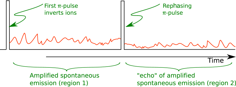
Figure 1: The RASE scheme. The first $\pi$-pulse shifts the two-level atoms into their excited state. Spontaneous emission from the excited atom ensemble produces the amplified spontaneous emission (ASE). During this emission, the atoms continually dephase due to inhomogeneous broadening. The rephasing $\pi$-pulse inverts the excitation of and rephases the atoms. Atoms that contributed to the ASE continue to emit photons to produce the RASE. This results in RASE that is a time-reversed “echo” of the ASE. The RASE and ASE are correlated at times equally spaced from the rephasing $\pi$-pulse.

Realization of the RASE scheme has been demonstrated in two separate systems. One system follows the original proposal [29] and the other [30] implements a modified approach based on four-level atoms [31]. Both demonstrations show that correlations exist between the ASE field and the RASE field. In the case of [29] the correlation was strong enough and the noise was low enough to show evidence of entanglement, although the confidence level was not high.

As a source of entanglement, RASE as it was initially proposed in [28] and [31] is imperfect. The main problem is the efficiency of the recall of entanglement from the atomic ensemble. In the first step of [28] illustrated in figure 1, an inverted ensemble of atoms creates ASE. This light is entangled with collective degrees of freedom of the atomic ensemble. The excitation in those collective degrees of freedom is then recalled into an output light field with a rephasing $\pi$-pulse. The fact that the quality of entanglement was limited by this recall efficiency is problematic. The low optical depths desirable in the first step to get weak ASE lead to poor recall efficiency. The four-level RASE [31] is slightly better in that separate transitions are used for the ASE and RASE steps. This means that a weak transition can be used for the ASE step and a stronger one for the RASE. Recently [32] further improvement has been suggested by tailoring the spatial density of the ions.

The recall efficiency of the RASE scheme can be improved by placing the atoms inside a low finesse cavity, an approach also used in quantum memories [33, 27, 34]. In this paper we examine this process of cavity enhanced rephased amplified spontaneous emission (CRASE). We will show that in the appropriate regime the CRASE scheme is capable of achieving a recall efficiency of 100%, and in principle perfect multimode, time-separated entanglement.

2 The Hamiltonian for our system

The evolution of CRASE is qualitatively the same as the RASE evolution shown in figure 1. The interaction picture Hamiltonian for our system takes the form (making the rotating wave approximation and setting $\hbar\equiv 1$)

$$H=H_{1}+H_{2}$$ (1)

where

$$H_{1}=\sum_{k=1}^{N}\sigma_{+}^{k}(t)\sigma_{-}^{k}(t)+\rmi g\sum_{k=1}^{N}(\sigma^{k}_{+}(t)a(t)-\sigma^{k}_{-}(t)a^{\dagger}(t))$$ (2)

is the usual Jaynes-Cummings Hamiltonian that models the interaction between $N$ two-level atoms and the cavity mode and

$$H_{2}=\int_{-\infty}^{\infty}\Delta b^{\dagger}(\Delta,t)b(\Delta,t)\,\rmd\Delta+\rmi\int_{-\infty}^{\infty}\kappa(\Delta)\left(b^{\dagger}(\Delta,t)a(t)-b(\Delta,t)a^{\dagger}(t)\right)\,\rmd\Delta$$ (3)

models the interaction between the external radiation field and the cavity [35, 36]. The operators $\sigma^{k}_{+}(t)$ and $\sigma^{k}_{-}(t)$ are raising and lowering operators respectively for atom $k$, $a(t)$ is the destruction operator for the cavity mode, $g$ is the coupling between the atoms and the cavity mode, which we take to be uniform, $b(\Delta,t)$ are destruction operators for the external radiation modes, $\Delta$ is the detuning from the cavity mode frequency and $\kappa(\Delta)$ is the coupling between the radiation mode with detuning $\Delta$ and the cavity mode.

3 The ASE field

At the beginning of region 1 in figure 1 the atoms are in their excited state. Spontaneous emission by the atoms produces the ASE field. We will assume that the atoms are weakly coupled to the cavity (small $g$) so that the atoms remain predominantly in their excited state throughout region 1. This allows us to approximate each atom as an inverted harmonic oscillator by setting $\sigma_{+}^{k}(t)\rightarrow s_{k}(t)$, where $s_{k}(t)$ are destruction operators satisfying $[s_{k}(t),s_{k^{\prime}}^{\dagger}(t)]=\delta_{kk^{\prime}}$ [35]. Like the ordinary harmonic oscillator, the eigenstates of an inverted harmonic oscillator form a ladder of equally spaced energy states. The ladder is inverted in the sense that an energy eigenstate $\ket{n}$ contains $n$ units of negative energy so that the state $\ket{n+1}\propto s_{k}^{\dagger}\ket{n}$ has a lower energy than the state $\ket{n}$. We will also approximate the collection of harmonic oscillators by a continuous field by setting $\sqrt{N}s_{k}(t)\rightarrow s(\Delta,t)$. The operators $s(\Delta,t)$ are destruction operators for a collective excitation across oscillators with detuning $\Delta$ and satisfy $[s(\Delta,t),s^{\dagger}(\Delta^{\prime},t)]=\delta(\Delta-\Delta^{\prime})$ in the limit $N\rightarrow\infty$. The Hamiltonian $H_{1}$ then takes the form

$$H_{1}=-\int_{-\infty}^{\infty}\Delta s^{\dagger}(\Delta,t)s(\Delta,t)\,\rmd\Delta+\rmi\int_{-\infty}^{\infty}g(\Delta)\left(s(\Delta,t)a(t)-s^{\dagger}(\Delta,t)a^{\dagger}(t)\right)\,\rmd\Delta$$ (4)

where $\sqrt{N}g\rightarrow g(\Delta)$.

Input-output theory [35] is often used when describing quantum systems interacting with a continuum of radiation modes, such as the situation described by equation (3). The interaction between the excited state atoms and the cavity mode, described by equation (4), is very similar: in both cases the cavity is interacting with a continuum of harmonic oscillators. This allows us to use input-output theory for the atom-cavity interaction also.

Following the standard input-output treatment we assume $\kappa(\Delta)$ and $g(\Delta)$ are slowly varying for our range of frequencies of interest. We can then make the first Markov approximation by setting $\kappa(\Delta)\rightarrow\kappa(0)\equiv\sqrt{\gamma_{\text{b,1}}/2\pi}$ and $g(\Delta)\rightarrow g(0)\equiv\sqrt{\gamma_{\text{a,1}}/2\pi}$. In the case of $g$, this is valid when the inhomogeneous broadening of the atoms is much broader than the cavity bandwidth. The loss rate of the bare cavity is $\gamma_{\text{b,1}}$. We call $\gamma_{\text{a,1}}$ the ‘gain rate’ of the cavity; this is the rate describing the exponential growth of light in the cavity if the cavity mirrors were perfect. We will work in the regime where $\gamma_{\text{a,1}}<\gamma_{\text{b,1}}$ so that we are below the lasing threshold.

We are now able to obtain an expression for the output ASE field. Solving the Heisenberg equations of motion for $b(\Delta,t)$, $s(\Delta,t)$ and $a(t)$ gives

$$b(\Delta,t)=\exp\left[-\rmi\Delta(t-t_{0})\right]b(\Delta,t_{0})+\sqrt{\frac{\gamma_{\text{b,1}}}{2\pi}}\int_{t_{0}}^{t}\exp\left[-\rmi\Delta(t-\tau)\right]a(\tau)\,\rmd\tau$$ (5)

$$s(\Delta,t)=\exp\left[\rmi\Delta(t-t_{0})\right]s(\Delta,t_{0})-\sqrt{\frac{\gamma_{\text{a,1}}}{2\pi}}\int_{t_{0}}^{t}\exp\left[\rmi\Delta(t-\tau)\right]a^{\dagger}(\tau)\,\rmd\tau$$ (6)

and

$$\eqalign{a(t)=-\int_{t_{0}}^{t}\exp\left[-\frac{\gamma_{\text{b,1}}-\gamma_{\text{a,1}}}{2}(t-\tau)\right]\left(\sqrt{\gamma_{\text{b,1}}}b_{\text{in}}(\tau)+\sqrt{\gamma_{\text{a,1}}}s_{\text{in}}^{\dagger}(\tau)\right)\,\rmd\tau\\ +\exp\left[-\frac{\gamma_{\text{b,1}}-\gamma_{\text{a,1}}}{2}(t-t_{0})\right]a(t_{0})}$$ (9)

where

$$b_{\text{in}}(t)\equiv\frac{1}{\sqrt{2\pi}}\int_{-\infty}^{\infty}\exp\left[-\rmi\Delta(t-t_{0})\right]b(\Delta,t_{0})\,\rmd\Delta$$ (10)

is the radiation field that enters the cavity at time $t$ and

$$s_{\text{in}}(t)\equiv\frac{1}{\sqrt{2\pi}}\int_{-\infty}^{\infty}\exp\left[\rmi\Delta(t-t_{0})\right]s(\Delta,t_{0})\,\rmd\Delta$$ (11)

is the input atomic field. Time $t_{0}<0$ occurs at the beginning of region 1 in figure 1. Both input fields are vacuum fields with $\left<b^{\dagger}(\Delta,t_{0})b(\Delta^{\prime},t_{0})\right>=\left<s^{\dagger}(\Delta,t_{0})s(\Delta^{\prime},t_{0})\right>=0$. Note that we name the input atomic field from the point of view of the cavity mode; the input atomic field is the field that drives the cavity mode. Equations (5) and (6) can be used to derive the relations [35]

$$b_{\text{ASE}}(t)\equiv b_{\text{out}}(t)=b_{\text{in}}(t)+\sqrt{\gamma_{\text{b,1}}}a(t)$$ (12)

$$s_{\text{out}}(t)=s_{\text{in}}(t)-\sqrt{\gamma_{\text{a,1}}}a^{\dagger}(t)$$ (13)

where

$$b_{\text{out}}(t)\equiv\frac{1}{\sqrt{2\pi}}\int_{-\infty}^{\infty}\exp\left(-\rmi\Delta t\right)b(\Delta,0)\,\rmd\Delta$$ (14)

is the ASE field - the radiation field that exits the cavity at time $t$ - and

$$s_{\text{out}}(t)\equiv\frac{1}{\sqrt{2\pi}}\int_{-\infty}^{\infty}\exp\left(\rmi\Delta t\right)s(\Delta,0)\,\rmd\Delta$$ (15)

is the output atomic field. The output atomic field is a collective de-excitation of atoms, or equivalently an excitation of the inverted harmonic oscillator field.

We will assume that the frequencies of interest of the ASE field is narrowband compared to $\gamma_{\text{b,1}}-\gamma_{\text{a,1}}$, the net loss rate of the cavity (see the implementation section for further discussion). We can then adiabatically eliminate the cavity mode, replacing $b_{\text{in}}(\tau)$ by $b_{\text{in}}(t)$ and $s_{\text{in}}(\tau)$ by $s_{\text{in}}(t)$ in equation (9). Substituting the resulting expression for $a(t)$ into equations (12) and (13) and letting $t_{0}\rightarrow-\infty$ gives the following input-output relations:

$$b_{\text{ASE}}(t)=-\frac{\gamma_{\text{b,1}}+\gamma_{\text{a,1}}}{\gamma_{\text{b,1}}-\gamma_{\text{a,1}}}b_{\text{in}}(t)-\frac{2\sqrt{\gamma_{\text{b,1}}\gamma_{\text{a,1}}}}{\gamma_{\text{b,1}}-\gamma_{\text{a,1}}}s_{\text{in}}^{\dagger}(t)$$ (16)

$$s_{\text{out}}(t)=\frac{\gamma_{\text{b,1}}+\gamma_{\text{a,1}}}{\gamma_{\text{b,1}}-\gamma_{\text{a,1}}}s_{\text{in}}(t)+\frac{2\sqrt{\gamma_{\text{b,1}}\gamma_{\text{a,1}}}}{\gamma_{\text{b,1}}-\gamma_{\text{a,1}}}b_{\text{in}}^{\dagger}(t)$$ (17)

These relations allow us to determine the output ASE field and output atomic field from the known input radiation and atomic fields.

4 The rephasing $\pi$-pulse

The rephasing $\pi$-pulse (applied at $t=0$) induces the following changes in our atoms [37]:

$$\sigma^{k}_{z}(0)\rightarrow-\sigma_{z}^{k}(\delta t)$$ (18)

$$\sigma_{+}^{k}(0)\rightarrow\sigma_{-}^{k}(\delta t)$$ (19)

where $\delta t$ is the duration of the $\pi$-pulse and $\sigma_{z}^{k}(t)=2\sigma_{+}^{k}(t)\sigma_{-}^{k}(t)-I$, where $I$ is the identity operator. The $\pi$-pulse inverts the excitation of and rephases the atoms. Like in [28], we model the rephasing pulse as an instantaneous $\pi$-pulse and so take $\delta t\rightarrow 0$. This is valid if $(\delta t)^{-1}$ is large compared to the bandwidth of the ASE and RASE fields that we are interested in.

5 The RASE field

After the rephasing $\pi$-pulse the atoms are predominantly in their ground state (equation (18)). But the atoms that fell to their ground state in region 1 will be in their excited state and these atoms produce the RASE field. Because the atoms are only weakly excited we approximate the atoms as a field of ordinary harmonic oscillators by setting $\sigma_{-}(\Delta,t)\rightarrow d(\Delta,t)$. Here $d(\Delta,t)$ are destruction operators satisfying $[d(\Delta,t),d^{\dagger}(\Delta^{\prime},t)]=\delta(\Delta-\Delta^{\prime})$.

The interaction picture Hamiltonian for our system takes the form (making the rotating wave approximation and setting $\hbar\equiv 1$)

$$\eqalign{H&=\int_{-\infty}^{\infty}\Delta b^{\dagger}(\Delta,t)b(\Delta,t)\,\rmd\Delta+\rmi\sqrt{\frac{\gamma_{\text{b,2}}}{2\pi}}\int_{-\infty}^{\infty}\left(b^{\dagger}(\Delta,t)a(t)-b(\Delta,t)a^{\dagger}(t)\right)\,\rmd\Delta\\ &\phantom{equals}+\int_{-\infty}^{\infty}\Delta d^{\dagger}(\Delta,t)d(\Delta,t)\,\rmd\Delta+\rmi\sqrt{\frac{\gamma_{\text{a,2}}}{2\pi}}\int_{-\infty}^{\infty}\left(d^{\dagger}(\Delta,t)a(t)-d(\Delta,t)a^{\dagger}(t)\right)\,\rmd\Delta}$$ (22)

The loss rate of the bare cavity is $\gamma_{\text{b,1}}$ and $\gamma_{\text{a,1}}$ is the rate the atoms would absorb photons from the cavity if the cavity mirrors were perfect. We have allowed for the atom-cavity and radiation-cavity couplings to differ from the couplings for times $t<0$. This allows for the case where either the $Q$-factor of the cavity changes or the oscillator strength of the atomic transition used for the ASE and RASE are different [31].

We again make the first Markov approximation and assume that the frequencies of interest of the RASE field is narrowband compared to $\gamma_{\text{a,2}}+\gamma_{\text{b,2}}$, the total loss rate of the cavity, allowing us to again adiabatically eliminate the cavity mode. Carrying out analogous calculations to those from the previous section we obtain the following input-output relations:

$$b_{\text{RASE}}(t)\equiv b_{\text{out}}(t)=-\frac{\gamma_{\text{b,2}}-\gamma_{\text{a,2}}}{\gamma_{\text{b,2}}+\gamma_{\text{a,2}}}b_{\text{in}}(t)-\frac{2\sqrt{\gamma_{\text{b,2}}\gamma_{\text{a,2}}}}{\gamma_{\text{b,2}}+\gamma_{\text{a,2}}}d_{\text{in}}(t)$$ (23)

$$d_{\text{out}}(t)=\frac{\gamma_{\text{b,2}}-\gamma_{\text{a,2}}}{\gamma_{\text{b,2}}+\gamma_{\text{a,2}}}d_{\text{in}}(t)-\frac{2\sqrt{\gamma_{\text{b,2}}\gamma_{\text{a,2}}}}{\gamma_{\text{b,2}}+\gamma_{\text{a,2}}}b_{\text{in}}(t)$$ (24)

where

$$b_{\text{RASE}}(t)\equiv\frac{1}{\sqrt{2\pi}}\int_{-\infty}^{\infty}\exp\left[-\rmi\Delta(t-t_{1})\right]b(\Delta,t_{1})\,\rmd\Delta$$ (25)

is the output RASE field, where $t_{1}$ is any time far in the future,

$$d_{\text{out}}(t)\equiv\frac{1}{\sqrt{2\pi}}\int_{-\infty}^{\infty}\exp\left[-\rmi\Delta(t-t_{1})\right]d(\Delta,t_{1})\,\rmd\Delta$$ (26)

is the output atomic field,

$$d_{\text{in}}(t)\equiv\frac{1}{\sqrt{2\pi}}\int_{-\infty}^{\infty}\exp\left(-\rmi\Delta t\right)d(\Delta,0)\,\rmd\Delta$$ (27)

is the input atomic field and $b_{\text{in}}(t)$ is defined by equation (10).

Equation (23) gives the RASE field as a function of the known input radiation field and the currently unknown input atomic field. The input atomic field for region 2 can be related to the output atomic field from region 1 using equation (19) with $\sigma_{+}^{k}(0)\rightarrow s(\Delta,0)$ and $\sigma_{-}^{k}(\delta t)\rightarrow d(\Delta,\delta t)$. The definitions of $d_{\text{in}}(t)$ and $s_{\text{out}}(t)$ (equations (27) and (15)) then give that

$$d_{\text{in}}(t)={s_{\text{out}}}(-t)$$ (28)

in the limit $\delta t\rightarrow 0$. Equation (28) shows that the input atomic field that drives the cavity mode after the rephasing pulse is equal to the output atomic field that was driven by the cavity mode before the rephasing pulse. Entanglement between $s_{\text{out}}(t)$ and $b_{\text{ASE}}(t)$ before the rephasing pulse is translated into entanglement between $d_{\text{in}}(t)$ and $b_{\text{ASE}}(-t)$ as a result of equation (28). The field $b_{\text{RASE}}(t)$ becomes entangled with $d_{\text{in}}(t)$ and is therefore also entangled with $b_{\text{ASE}}(-t)$.

Using equations (28) and (17) in equation (23) gives

$$b_{\text{RASE}}(t)=-\frac{\gamma_{\text{b,2}}-\gamma_{\text{a,2}}}{\gamma_{\text{b,2}}+\gamma_{\text{a,2}}}b_{\text{in}}(t)-\frac{2\sqrt{\gamma_{\text{b,2}}\gamma_{\text{a,2}}}}{\gamma_{\text{b,2}}+\gamma_{\text{a,2}}}\left(\frac{\gamma_{\text{b,1}}+\gamma_{\text{a,1}}}{\gamma_{\text{b,1}}-\gamma_{\text{a,1}}}s_{\text{in}}(-t)+\frac{2\sqrt{\gamma_{\text{b,1}}\gamma_{\text{a,1}}}}{\gamma_{\text{b,1}}-\gamma_{\text{a,1}}}b_{\text{in}}^{\dagger}(-t)\right)$$ (29)

and this along with equation (16) give the RASE and ASE fields as functions of the input atomic field before the rephasing pulse and input radiation field. The input-output relations describing our system are shown graphically in figure 2.

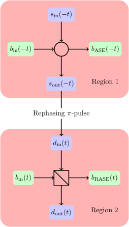
Figure 2: Graphical representation of the input-output relations (16) and (29). In the time region 1 the input optical field $b_{\text{in}}(-t)$ and the input atomic field $s_{\text{in}}(-t)$ combine like in a non-degenerate parametric amplifier to produce the outputs $b_{\text{ASE}}(-t)$ and $s_{\text{out}}(-t)$. The rephasing pulse means that the input atomic field for region 2 ($d_{\text{in}}(t)$) matches the output atomic field from region 1 ($s_{\text{out}}(-t)$) . In region 2, the optical and atomic fields interact like on a beamsplitter. For an impedance matched cavity the reflectivity of this beamsplitter is 1. It is well known that in an impedance matched cavity full of atoms any input field gets totally absorbed by the atoms, and none of it escapes as light. What also happens in an impedance matched cavity is that the input atomic field is completely mapped onto the output optical field leading to 100% recall efficiency. This means that if the cavity is impedance matched in region 2, the two output optical fields $b_{\text{ASE}}(-t)$ and $b_{\text{RASE}}(t)$ will be maximally entangled.

6 Quantifying entanglement

To concentrate on a single temporal mode for both the ASE and RASE fields we introduce mode operators $A$ and $B$ defined by

$$A\equiv-\int_{-\infty}^{0}g(t)b_{\text{ASE}}(t)\,\rmd t$$ (30)

$$B\equiv\int_{0}^{\infty}g(t)^{*}b_{\text{RASE}}(t)\,\rmd t$$ (31)

where $g(t)$ is a temporal mode function satisfying $g(-t)=g(t)$ and $\int_{0}^{\infty}|g(t)|^{2}\,\rmd t=1$. The number of photons in the ASE and RASE modes are then given by $N_{\text{ASE}}=\left<A^{\dagger}A\right>$ and $N_{\text{RASE}}=\left<B^{\dagger}B\right>$

Equations (16) and (29) give that

$$A=A_{0}\cosh\chi+B_{0}^{\dagger}\sinh\chi$$ (32)

$$B=\sqrt{\epsilon}C_{0}-\sqrt{1-\epsilon}\left(B_{0}\cosh\chi+A_{0}^{\dagger}\sinh\chi\right)$$ (33)

where $A_{0}\equiv\int_{-\infty}^{0}g(t)b_{\text{in}}(t)\,\rmd t$, $B_{0}\equiv\int_{-\infty}^{0}g(t)^{*}s_{\text{in}}(t)\,\rmd t$, $C_{0}\equiv-\int_{0}^{\infty}g(t)^{*}b_{\text{in}}(t)\,\rmd t$, $\cosh\chi\equiv(\gamma_{\text{b,1}}+\gamma_{\text{a,1}})/(\gamma_{\text{b,1}}-\gamma_{\text{a,1}})$ and $\sqrt{\epsilon}\equiv(\gamma_{\text{b,2}}-\gamma_{\text{a,2}})/(\gamma_{\text{b,2}}+\gamma_{\text{a,2}})$. We have that $[c_{j},c_{k}^{\dagger}]=\delta_{jk}$ and $\left<c_{j}^{\dagger}c_{k}\right>=0$, with $c_{j}\in\left\{A_{0},B_{0},C_{0}\right\}$. Equations (32) and (33) take the form of the equations describing the output of a non-degenerate parametric amplifier and beam splitter combination [38], see figure 2.

Equations (32) and (33) give that $N_{\text{ASE}}=\sinh^{2}\chi$ and $N_{\text{RASE}}=(1-\epsilon)\sinh^{2}\chi$. The recall efficiency of our system is given by $N_{\text{RASE}}/N_{\text{ASE}}=1-\epsilon$. If the cavity is impedance matched in region 2 ($\gamma_{\text{a,2}}=\gamma_{\text{b,2}}$) the recall efficiency is 100%, resulting in perfect entanglement between the ASE and RASE fields.

We will quantify the entanglement between the ASE and RASE fields using the criterion of Duan et al. [39]. For this criterion we introduce the operators

$$u\equiv\sqrt{\theta}x_{\text{A}}+\sqrt{1-\theta}x_{\text{B}}$$ (34)

$$v\equiv\sqrt{\theta}p_{\text{A}}-\sqrt{1-\theta}p_{\text{B}}$$ (35)

where $x_{c}\equiv(c+c^{\dagger})/\sqrt{2}$ and $p_{c}\equiv-\rmi(c-c^{\dagger})/\sqrt{2}$ are amplitude and phase quadrature fields satisfying $[x_{c},p_{c^{\prime}}]=\rmi\delta_{cc^{\prime}}$, with $c,c^{\prime}\in\left\{\text{A},\text{B}\right\}$, and $\theta$ can be any real number in the interval $(0,1)$. Then a sufficient condition for entanglement between the ASE and RASE photons is that $\left<\Delta u^{2}\right>+\left<\Delta v^{2}\right><1$ . Figure 3 shows a contour plot of $\left<\Delta u^{2}\right>+\left<\Delta v^{2}\right>$, minimised with respect to $\theta$, versus $\sqrt{\epsilon}$ and $\cosh\chi$. The ASE and RASE fields are entangled for all parameter values considered in this figure.

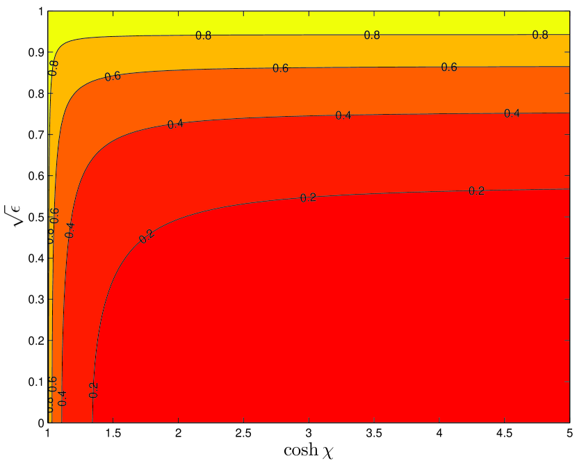
Figure 3: Contour plot of $\left<\Delta u^{2}\right>+\left<\Delta v^{2}\right>$, minimised with respect to $\theta$, versus $\sqrt{\epsilon}$ and $\cosh\chi$. The ASE and RASE fields are necessarily entangled in regions where $\left<\Delta u^{2}\right>+\left<\Delta v^{2}\right><1$. The ASE and RASE fields are entangled for all parameter values considered in this figure.

It can be shown that for our system

$$\left<\Delta u^{2}\right>+\left<\Delta v^{2}\right>=1+2\sinh^{2}\chi-2\epsilon(1-\theta)\sinh^{2}\chi-4\sqrt{\theta-\theta^{2}}\sqrt{1-\epsilon}\cosh\chi\sinh\chi$$ (36)

Setting $\theta=(1-\epsilon)/(2-\epsilon)$ gives $\left<\Delta u^{2}\right>+\left<\Delta v^{2}\right><1$ for all valid values of $\chi$ and $\epsilon$. Therefore the ASE and RASE fields are entangled for all valid parameter values.

7 Implementation

To implement our proposal, it is necessary to use two-level atoms with coherence times longer than the combined duration of the ASE and RASE fields. This could be achieved using the long coherence time of rare-earth doped solids [40] or by using Raman transitions in atomic gases [41].

Operation with the cavity impedance matched in region 2 requires either some way of changing the atom oscillator strength, such as the four-level scheme of [31], or a $Q$-switched cavity because, in order not to cross the lasing threshold, $\gamma_{\text{b,1}}>\gamma_{\text{a,1}}$ is required in region 1. In the case of the four-level scheme, the atom-cavity coupling in regions 1 and 2 can be made to differ by a factor $\gtrsim 10$ using appropriate rare-earth materials [42, 43]. In the case of $Q$-switching, it is not satisfactory to simply insert a variable attenuator, as attenuation introduces an unwanted additional output port that reduces the photon recall efficiency. Instead, various methods of active $Q$-switching can be used that do not introduce unwanted loss: using AOM or EOM components allows for variable control of the output field [44, 45]; the output of a WGM resonator coupled to an optical fiber or prism can be varied by changing the distance between the WGM resonator and the fiber or prism [46, 47]; or a thin Fabry-Pérot resonator with variable mirror separation can be used as a mirror with a variable reflectivity [48].

The cavity finesses required for implementation are only moderate, being no larger than that required to achieve impedance matching. This does not pose a great challenge, since the atomic absorption can be made much larger than the limit of current cavity decay rates.

The bandwidth of the output light is determined by either the cavity linewidth or the width of the inhomogeneous broadening. We will only be interested in a band of this light that is narrow compared to $\min\left(\gamma_{\text{b,1}}-\gamma_{\text{a,1}},\gamma_{\text{b,2}}+\gamma_{\text{a,2}}\right)$, since adiabatic elimination of the cavity dynamics is only valid for such a range. Filtering this narrowband signal from the full bandwidth of the output light can be achieved in a number of ways. The easiest to implement is homodyne or heterodyne detection [49]. In this way the filtering problem is reduced to filtering electrical signals. This method is suitable for quantum repeaters using a continuous variable basis [50, 51]. For quantum repeaters using a discrete Fock basis, filtering using standard techniques such as Fabry-Pérot etalons is a possibility, and when using rare-earth ions one can also use the array of narrow band filtering techniques recently developed based on spectral holeburning [52, 53].

It has been assumed that the rephasing $\pi$-pulse is a perfect $\pi$-pulse. The feasibility of applying a $\pi$-pulse to the whole ensemble is greatly helped by the area theorem [54], which states that a $\pi$-pulse will remain a $\pi$-pulse as it travels through resonant media. This has strong analogues in a cavity [55]. Of course, in practice the $\pi$-pulse won’t be perfect. An imperfect $\pi$ pulse can be considered as a combination of a perfect $\pi$ pulse and a small perturbing pulse. The small perturbing pulse adds unwanted excitation to the atomic field, which adds noise to the RASE field. However, as discussed in [28], this noise disappears shortly after the $\pi$ pulse, since the unwanted excitation of the atomic field will be temporally brief and will rapidly dephase and no longer interact with the cavity mode. The variation in driving strength of the atoms due to variations in the cavity mode field intensity could be removed using hole burning techniques [56, 57].

8 Conclusion

In conclusion, we have analysed rephased amplified spontaneous emission with the atoms placed in an optical cavity. The cavity can alleviate the problem of low recall efficiency, particularly if the cavity is impedance matched when the entangled light is being recalled from the atoms, in which case the recall will theoretically be perfect. Achieving the impedance matched condition during recall requires either a $Q$-switched cavity or some way of switching the atoms’ oscillator strengths, such as in the four-level scheme of Beavan et al. [31], since the ASE field has to be produced below the lasing threshold. We have also shown that entanglement exists between the ASE and RASE fields for all valid parameter values. Theoretically, our system has the potential to achieve time-separated entanglement with perfect recall efficiency, which is indispensable in producing an effective quantum repeater.

References

References

- [1] Briegel H J, Dür W, Cirac J I and Zoller P 1998 Phys. Rev. Lett. 81 5932
- [2] Duan L M, Lukin M D, Cirac J I and Zoller P 2001 Nature 414 413–418
- [3] Matsukevich D, Chaneliere T, Bhattacharya M, Lan S Y, Jenkins S, Kennedy T and Kuzmich A 2005 Phys. Rev. Lett. 95 040405
- [4] Felinto D, Chou C W, Laurat J, Schomburg E W, de Riedmatten H and Kimble H J 2006 Nature Phys. 2 844 – 848
- [5] Chanelière T, Matsukevich D N, Jenkins S D, Lan S Y, Zhao R, Kennedy T A B and Kuzmich A 2007 Phys. Rev. Lett. 98(11) 113602
- [6] Yuan Z S, Chen Y A, Chen S, Zhao B, Koch M, Strassel T, Zhao Y, Zhu G J, Schmiedmayer J and Pan J W 2007 Phys. Rev. Lett. 98(18) 180503
- [7] Laurat J, Choi K, Deng H, Chou C and Kimble H 2007 Phys. Rev. Lett. 99 180504
- [8] Yuan Z S, Chen Y A, Zhao B, Chen S, Schmiedmayer J and Pan J W 2008 Nature 454 1098–1101
- [9] Choi K S, Deng H, Laurat J and Kimble H 2008 Nature 452 67–71
- [10] Clausen C, Usmani I, Bussières F, Sangouard N, Afzelius M, de Riedmatten H and Gisin N 2011 Nature 469 508–511
- [11] Moiseev S and Kröll S 2001 Phys. Rev. Lett. 87 173601–173604
- [12] Moiseev S, Tarasov V and Ham B 2003 J. Opt. B: Quantum Semiclass. Opt. 5 S497
- [13] Nilsson M and Kröll S 2005 Opt. Commun. 247 393–403
- [14] Kraus B, Tittel W, Gisin N, Nilsson M, Kröll S and Cirac J 2006 Phys. Rev. A 73 020302
- [15] Afzelius M, Chaneliere T, Cone R L, Kröll S, Moiseev S A, Sellars M et al. 2010 Laser Photon. Rev. 4 244–267
- [16] Hosseini M, Sparkes B M, Hétet G, Longdell J J, Lam P K and Buchler B C 2009 Nature 461 241–245
- [17] Hedges M P, Longdell J J, Li Y and Sellars M J 2010 Nature 465 1052–1056
- [18] Afzelius M, Usmani I, Amari A, Lauritzen B, Walther A, Simon C, Sangouard N, Minář J, De Riedmatten H, Gisin N et al. 2010 Phys. Rev. Lett. 104 040503
- [19] Saglamyurek E, Sinclair N, Jin J, Slater J A, Oblak D, Bussières F, George M, Ricken R, Sohler W and Tittel W 2011 Nature 469 512–515
- [20] Hosseini M, Campbell G, Sparkes B, Lam P and Buchler B 2011 Nature Phys. 7 794–798
- [21] Sabooni M, Li Q, Kröll S and Rippe L 2013 Phys. Rev. Lett. 110(13) 133604
- [22] Gündoğan M, Mazzera M, Ledingham P M, Cristiani M and de Riedmatten H 2013 New J. Phys. 15 045012
- [23] Timoney N, Usmani I, Jobez P, Afzelius M and Gisin N 2013 Phys. Rev. A 88 022324
- [24] Bonarota M, Dajczgewand J, Louchet-Chauvet A, Gouët J L L and Chaneliere T 2013 arXiv:1311.7331
- [25] Jobez P, Usmani I, Timoney N, Laplane C, Gisin N and Afzelius M 2014 arXiv:1404.3489
- [26] Simon C, De Riedmatten H, Afzelius M, Sangouard N, Zbinden H and Gisin N 2007 Phys. Rev. Lett. 98 190503
- [27] Moiseev S A, Andrianov S N and Gubaidullin F F 2010 Phys. Rev. A 82(2) 022311
- [28] Ledingham P M, Naylor W R, Longdell J J, Beavan S E and Sellars M J 2010 Phys. Rev. A 81(1) 012301
- [29] Ledingham P M, Naylor W R and Longdell J J 2012 Phys. Rev. Lett. 109(9) 093602
- [30] Beavan S E, Hedges M P and Sellars M J 2012 Phys. Rev. Lett. 109(9) 093603
- [31] Beavan S E, Ledingham P M, Longdell J J and Sellars M J 2011 Opt. Lett. 36 1272–1274
- [32] Stevenson R N, Hush M R, Carvalho A R, Beavan S E, Sellars M J and Hope J J 2013 arXiv:1311.4957
- [33] Afzelius M and Simon C 2010 Phys. Rev. A 82(2) 022310
- [34] Sabooni M, Li Q, Kröll S and Rippe L 2013 Phys. Rev. Lett. 110(13) 133604
- [35] Gardiner C and Zoller P 2004 Quantum Noise (Springer)
- [36] Dutra S M 2005 Cavity Quantum Electrodynamics (Wiley)
- [37] Allen L and Eberly J 1975 Optical Resonance and Two-Level Atoms vol 28 (Wiley)
- [38] Walls D and Milburn G 1995 Quantum Optics (Springer)
- [39] Duan L, Giedke G, Cirac J I and Zoller P 2000 Phys. Rev. Lett. 84 2722
- [40] Thiel C, Böttger T and Cone R 2011 J. Lumin. 131 353–361
- [41] Hétet G, Hosseini M, Sparkes B, Oblak D, Lam P K and Buchler B C 2008 Opt. Lett. 33 2323–2325
- [42] Nilsson M, Rippe L, Kröll S, Klieber R and Suter D 2004 Phys. Rev. B 70 214116
- [43] Guillot-Noël O, Goldner P, Beaudoux F, Le Du Y, Lejay J, Amari A, Walther A, Rippe L and Kröll S 2009 Phys. Rev. B 79 155119
- [44] Yariv A 1989 Quantum Electronics (Wiley)
- [45] Orazio S 1998 Principles of Lasers (Plenum Press)
- [46] Gorodetsky M L and Ilchenko V S 1999 J. Opt. Soc. Am. B 16 147–154
- [47] Gorodetsky M and Ilchenko V 1994 Opt. Commun. 113 133–143
- [48] Strain K and Hough J 1994 Rev. Sci. Instrum. 65 799–802
- [49] Yuen H P and Chan V W 1983 Opt. Lett. 8 177–179
- [50] Hage B, Samblowski A, DiGuglielmo J, Franzen A, Fiurášek J and Schnabel R 2008 Nature Phys. 4 915–918
- [51] Braunstein S L and van Loock P 2005 Rev. Mod. Phys. 77(2) 513–577
- [52] Li Y, Zhang H, Kim C, Wagner K H, Hemmer P and Wang L V 2008 Appl. Phys. Lett. 93 011111
- [53] McAuslan D, Taylor L and Longdell J 2012 Appl. Phys. Lett. 101 191112
- [54] McCall S L and Hahn E L 1969 Phys. Rev. 183 457
- [55] Chanelière T 2013 arXiv:1309.4669
- [56] Pryde G, Sellars M and Manson N 2000 Phys. Rev. Lett. 84 1152–1155
- [57] Longdell J and Sellars M 2004 Phys. Rev. A 69 032307