End states in a 1-D topological Kondo insulator

Abstract

To gain further insight into the properties of interacting topological insulators, we study a 1 dimensional model of topological Kondo insulators which can be regarded as the strongly interacting limit of the Tamm-Shockley model. Treating the model in a large $N$ expansion, we find a number of competing ground-state solutions, including topological insulating and valence bond ground-states. One of the effects to emerge in our treatment is a reconstruction of the Kondo screening process near the boundary of the material (“Kondo band bending” ). Near the boundary for localization into a valence bond state, we find that the conduction character of the edge state grows substantially, leading to states that extend deeply into bulk. We speculate that such states are the one-dimensional analog of the light f-electron surface states which appear to develop in the putative topological Kondo insulator, SmB₆.

I Introduction

Topological insulators Haldane1988 ; Fu2005 ; Kane2005 ; Kane2005_2 ; Fu2007 ; Moore2010 ; TIreview1 ; TIreview2 ; Moore2007 ; Roy2009 ; Qi2008 have attracted great attention as a new class of band insulator with gapless surface or edge states, robustly protected by combination of time-reversal symmetry and the non-trivial topological winding of the occupied one-particle wavefunctions. The surface states of a topological insulator are “massless” excitations carried by an odd number of Dirac cones in the Brillouin zone.

Various proposals have been made for strongly correlated electron analoguesWang2010 ; Dzero2010 ; Jiang2012 ; Nourafkan2013 ; Wang2012 ; Fidkowski2011 ; Wang2014 of topological band insulators. To date the best candidate strongly correlated topological insulator is SmB₆, a local moment metal which transforms into a Kondo insulator, once the moments screen at low temperatures ($<70K$) Geballe1969 . This material was first predicted to be a topological Kondo insulator Dzero2010 and recently shown to exhibit conducting in-gap surface states, which develop below $4$K exp1smb6 ; exp2smb6 ; exp3smb6 . While these results are consistent with a topological Kondo insulator, a definitive observation of Dirac cone excitations with polarized quasiparticles has not yet been reported. However, tentative data of the Dirac cone surface states have become available in both Quantum oscillation QuantumOsc2013 and ARPES measurementsHasan2013 ; ARPES2 ; ARPES3 ; ARPES4 . One of the unexpected features of these measurements is the presence of “light”, high-velocity surface quasiparticles, with the Dirac point far outside the gap. These tentative results are puzzling, because their group velocities appear 10 to 100 times larger than that expected in a heavy fermion band Dai2013 ; Alexandrov2013 .

These results provide motivation for the current paper. Here we introduce a simple one dimensional “p-wave Kondo lattice” which gives rise to a topological Kondo insulator that can be studied by a variety of methods. In this initial study we carry out the simplest mean-field treatment of our model, an approach which is technically exact in the large $N$ limit, using it to gain insight into the nature of the edge states and to propose variational ground-states for the model. This work is also an important warm-up exercise for a three dimensional model. The model is schematically depicted in Fig. 1. It can be regarded as a strongly interacting limit of Tamm-Shockley model Tamm1932 ; Shockley1939 ; Yakovenko2012 .

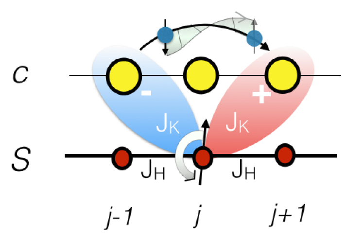
Figure 1: (Color online) Schematic illustration of the 1D p-wave Kondo insulator Hamiltonian (1). The model contains a chain of Heisenberg spins coupled by an antiferromagnetic nearest neighbor Heisenberg coupling, plus a tight-binding chain of conduction electrons (c). Each localized moment is coupled to the conduction sea via a Kondo “cotunneling” term that exchanges spin between a localized moment at site $j$ and a p-wave combination of conduction electron states formed between neighboring sites $j-1$ and $j+1$.

.

A second goal of this work is to gain insight into the the impact of the boundary on the Kondo effect, a phenomenon we refer to as “Kondo band bending”. In the conventional Kondo insulator model, the hybridization between local moments and conduction electrons is local and the strong-coupling ground state involves a Kondo singlet at every site, with minimal boundary effects. In the case of non-trivial topology the Kondo singlets are non-local objects (Fig. 1) which are partially broken at the boundary. We seek to understand how this influences the Kondo effect and the character of the edge states at the boundary.

II The model

Our model describes conduction electron fluid interacting with an antiferromagnetic Heisenberg spin chain via a Kondo co-tunneling term with p-wave character. The Hamiltonian is given by

$$H=H_{c}+H_{H}+H_{K},$$ (1)

where

$$H_{c} =-t\sum_{j,\sigma}(c_{j+1\sigma}^{\dagger}c_{j\sigma}+\rm H.c)$$ (2)

$$H_{H} =J_{H}\sum_{i}{\bf S}_{j}\cdot{\bf S}_{j+1},$$ (3)

$$H_{K} =\sum_{j,\alpha\beta}\frac{J_{K}{(j)}}{2}{\bf S}_{j}\!\cdot\!p_{j,\alpha}^{\dagger}{\boldsymbol{\sigma}}_{\alpha\beta}p_{j,\beta}.$$ (4)

Here the site index runs over the length of the chain, $j\in[1,L]$, $t$ is the nearest neighbor a hopping matrix element, $J_{H}$ is a nearest neighbor Heisenberg coupling and $J_{K}(j)$ is the Kondo coupling at site $j$. The chemical potential of the conduction electrons has been set to zero, corresponding to a half-filled conduction band. In contrast to the conventional ’s-wave’ Kondo model, the Kondo effect is non-local. In particular, the electron Wannier states that couple to the local moment have p-wave symmetry

$$p_{j,\sigma}\equiv c_{j+1,\sigma}-c_{j-1\sigma}.$$ (5)

The Kondo coupling now permits the process of “co-tunneling” whereby an electron can hop across a spin as it flips it. The odd-parity co-tunneling terms are a consequence of the underlying hybridization with localized p-wave orbitals. When this hybridization is eliminated via a Schrieffer-Wolff transformation, the resulting Kondo interaction contains an odd-parity form factor.

The boundary spins have a lower connectivity, giving rise to a lower Kondo temperature which tends to localize them into a magnetic state. To examine these effects in greater detail, we take the Kondo coupling $J_{K}(j)=J_{K}$ to be uniform in the bulk, but to have strength $\alpha J_{K}$ at the boundary,

$$J_{K}(j)=\left\{\begin{array}[]{ll}\alpha J_{K}&\hbox{endpoints}\ \ (j=1\hbox{\ or\ }L),\\ J_{K}&\hbox{bulk}\ (j\in[2,L-1]).\end{array}\right.$$ (6)

By allowing the end couplings to be enhanced by a factor $\alpha$ we can crudely compensate for the localizing effect of the reduced boundary connectivity. In real 3D Kondo insulators, this surface enhancement effect (“Kondo band-bending”) would occur in response to changes in the valence of the magnetic ions near the surface. For Sm and Yb Kondo insulators, the valence of the surface ions is expected to shift to a more mixed valent configuration, enhancing $\alpha$, while in Ce Kondo insulators, the opposite effect is expected.

To formulate the model as a canonical field theory, we rewrite the spin ${\bf S}_{j}$ using Abrikosov pseudo-fermions $f_{j\sigma}$, as

$${\bf S}_{j}=\sum_{\sigma\sigma^{\prime}}f{{}^{\dagger}}_{j\sigma}\boldsymbol{\sigma}_{\sigma\sigma^{\prime}}f_{j\sigma^{\prime}},$$ (7)

with the associated “Gutzwiller” constraint $n_{f,j}=1$ at each site. After applying the completeness relations for the Pauli matrices in (4) we obtain the Coqblin-Schrieffer form of the Kondo interaction,

$$H_{K}=-J_{K}\sum_{j,\alpha\beta}\left(f^{\dagger}_{j,\alpha}p_{i\alpha}\right)\left(p^{\dagger}_{j,\beta}f_{i\beta}\right)$$ (8)

where we have imposed the constraint. In an analogous fashion, the local moment interaction (3) can be re-written as

$$H_{H}=-J_{H}\sum_{j,\alpha\beta}(f^{\dagger}_{j+1,\alpha}f_{j\alpha})(f^{\dagger}_{j,\beta}f_{j+1\beta})$$ (9)

If we now cast the Hamiltonian inside a path integral, we can factorize the Kondo and Heisenberg interactions using a Hubbard-Stratonovich decoupling,

$$H\rightarrow H_{c}+\sum_{j,\sigma}\left(\bar{V}_{j}(c{{}^{\dagger}}_{j+1\sigma}-c{{}^{\dagger}}_{j-1\sigma})f_{j\sigma}+{\rm H.c}\right)+\frac{|V_{j}|^{2}}{J_{K}{(j)}}$$ (10)

$$\qquad+\sum_{j,\sigma}\left(\Delta_{j}f^{\dagger}_{j+1,\sigma}f_{j,\sigma}+\hbox{H.c}\right)+{|\Delta_{j}|^{2}\over J_{H}}$$ (11)

$$\qquad+\sum_{j}\lambda_{j}(n_{f,j}-1),$$ (12)

with the understanding that auxiliary fields $V_{i}$, $\Delta_{j}$ and $\lambda_{j}$ are fluctuating variables, integrated within a path integral. The last term imposes the constraint $n_{f,j}=1$ at each site.

In this formulation of the problem $V_{i}$ determines the Kondo hybridization on site $i$ and $\Delta_{i}$ is the order parameter for RVB-like state formed on the link $i$ between local moments. In translating our mean-field results back into the physical subspace of spins and electrons it is important to realize that the f-electron operators (which are absent in the original spin formulation of the model) represent composite fermions that result from the binding of spin flips to conduction electrons as part of the Kondo effect. By comparing (10) with (4), we see that the f-electron represents the following (three-body) contraction between conduction and spin operators:

$$\contraction{}{\bf S}{{}_{j}\cdot{\boldsymbol{\sigma}}_{\alpha\beta}\hskip-2.84526pt}{p}{\bf S}_{j}\cdot{\boldsymbol{\sigma}}_{\alpha\beta}p_{j,\beta} \equiv \left(\frac{2\bar{V}}{J_{K}}\right)f_{j,\alpha},$$ (13)

$$\contraction[2ex]{}{p{{}^{\dagger}}}{{}_{j,\beta}{\boldsymbol{\sigma}}_{\beta\alpha}\cdot\hskip-2.84526pt}{{\bf S}}p{{}^{\dagger}}_{j,\beta}{\boldsymbol{\sigma}}_{\beta\alpha}\cdot{\bf S}_{j} \equiv \left(\frac{2V}{J_{K}}\right)f{{}^{\dagger}}_{j,\alpha}.$$ (14)

At low energies, these bound-state objects behave as independent electron states, injected into the conduction sea to form a filled band and create a Kondo insulator.

II.1 Homogeneous mean field approximation

In the homogeneous mean field treatment of the Hamiltonian (10) we assume that the bulk fields $V_{j}$, $\Delta_{j}$ and $\lambda_{j}$ are constants. The saddle-point Hamiltonian then becomes a translationally invariant tight binding model. For periodic boundary conditions, taking $\Delta_{j}=\Delta$, $V_{j}=V$, we obtain

$$H=H_{TB}+L\left(\frac{|V|^{2}}{J_{K}}+\frac{|\Delta|^{2}}{J_{H}}-\lambda\right).$$ (15)

$H_{TB}$ can be written in momentum space as

$$H_{TB}=\sum_{k}(c_{k\sigma}^{\dagger},f_{k\sigma}^{\dagger})\overbrace{\begin{pmatrix}-2t\cos k&-2i\bar{V}\sin k\\ 2iV\sin k&2\Delta\cos k+\lambda\end{pmatrix}}^{H(k)}\begin{pmatrix}c_{k\sigma}\\ f_{k\sigma}\end{pmatrix}$$ (16)

This model is represented schematically in Fig. 2(a).

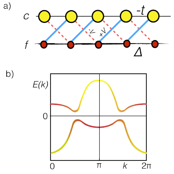
Figure 2: (Color online) Illustrating the tight-binding model. (a) Real space structure. (b) Dispersion of quasiparticles, showing band inversion at $k=\pi$(16)

II.2 Large $N$ limit

The mean-field treatment replaces the hard constraint $n_{f}=1$ by an average $\langle n_{f}\rangle=1$ at each site. This replacement becomes asymptotically exact in a large $N$ extension of the model, in in which the fermions have $N$ possible spin flavors, $\sigma\in[1,N]$. Provided all terms in the Hamiltonian grow extensively with N, the path integral can be rewritten with an effective Planck constant $\hbar_{\hbox{eff}}=1/N$ which suppresses quantum fluctuations as $N\rightarrow\infty$ and $\hbar_{\hbox{eff}}\rightarrow 0$. To scale the model so that the Hamiltonian grows extensively with $N$, we replace

$$J_{H}\rightarrow J_{H}/N,\quad\quad J_{K}\rightarrow J_{K}/N,$$ (17)

$$\sum_{j}\lambda(n_{f,j}-1)\rightarrow\sum_{j}\lambda(n_{f,j}-Q).$$ (18)

where the last term imposes $n_{f,j}=Q$ rather than unity at each site. We shall examine the case where $Q=N/2$, corresponding to a particle-hole symmetric Kondo lattice. We shall restrict our attention to solutions where $\lambda=0$, which gives rise to an insulating state in which both the conduction and f-bands are half-filled.

II.3 Topological class D

The mean-field Hamiltonian (16) can be classified according to the periodic table of free fermion topological phasesSchnyder2008 ; Qi2008 ; Kitaev2009 . The particle hole symmetry $\Xi:$ $\Xi H(k)\Xi^{\dagger}=-H^{T}(k)$ is equivalent to the transformation $c_{k}\rightarrow c_{\pi-k}^{\dagger}$, $f_{k}\rightarrow f_{\pi-k}{{}^{\dagger}}$. In the two band basis of Hamiltonian (16) $\Xi=\tau_{z}$, where $\tau$ denotes a Pauli matrix acting in orbital space. According to the periodic table, symmetric $\Xi$ corresponds to class D.

One way to see the non-trivial topology is to observe the evolution of the Hamiltonian throughout the Brillouin zone by writing it as a vector in three dimensional space: $H(k)=\vec{h}(k)\cdot\vec{\tau}+\epsilon_{0}(k)$ with $\epsilon_{0}(k)=(\Delta-t)\cos k$. For real $V$,

$$\vec{h}(k)=\left[\begin{array}[]{c}0\\ 2V\sin k\\ -(\Delta+t)\cos k\end{array}\right].$$

At $k=0$ and $k=\pi$, the vector $\vec{h}(k)$ aligns along the $\hat{z}$ axis: if the sign of the scalar product $\vec{h}(0)\cdot\vec{h}(\pi)$ of the two vectors is positive, vector $\vec{h}(k)$ traces a simply-connected path on the 2-sphere that may be contracted to a point, so the phase is topologically trivial. By contrast, a negative sign corresponds to a topologically non-trivial path that connects the poles of the sphere, indicating the topological phase. This can be surmised as

$$(-1)^{\nu}=\text{sign}(\vec{h}(0)\cdot\vec{h}(\pi)),$$ (19)

where $\nu=0$ for trivial and $\nu=1$ for topological phases. In our model $\vec{h}(0)\cdot\vec{h}(\pi)=-(t+\Delta)^{2}$ and hence $\nu=1$ for any uniform solution with finite $V$.

The consequence of the topological invariance can be seen in the non-zero electric polarization $P$. A particle-hole transformation reverses the polarization, and since the Hamiltonian is invariant under this transformation it follows that $\Xi P\Xi^{\dagger}=-P$, allowing only two possible values of polarization: $P=0$ or $P=e/2$ since $P$ is defined modulo $e$. This is in fact the topological index of the chain. P can be computed via the Berry connection $A_{k}=i\langle u_{k}|\partial_{k}|u_{k}\rangle$kingsmithvanderbilt of the occupied bands, defined via periodic part of the Bloch function, $u_{k}$.

$$P={e}\int_{0}^{2\pi}\frac{dk}{2\pi}A_{k}=\left\{\begin{array}[]{l l}e/2&\quad\text{topological}\\ 0&\quad\text{trivial}\end{array}\right.$$ (20)

The validity of this relation depends on the use of a smooth Berry connection $A_{k}$, which usually requires that we carry out a a gauge transformation on the raw eigenstates. For example, consider the special case where $t=\Delta=V$. The negative energy eigenstates then take the form $\psi_{k}=(\cos(k/2),-i\sin(k/2))e^{i\phi(k)}$: choosing $\phi(k)=k/2$, the eigenstates then become continuous. If the orbital basis is centro-symmetric, the Berry phase only depends on the $\psi_{k}$: $A_{k}=i\langle u_{k}|\partial_{k}|u_{k}\rangle=i\psi_{k}^{\dagger}\partial_{k}\psi_{k}$. Computing the Berry connection, we obtain

$$A_{k} =ie^{-ik/2}\left({\cos\frac{k}{2}},{i\sin\frac{k}{2}}\right)\partial_{k}\begin{pmatrix}\cos(k/2)\cr-i\sin(k/2)\end{pmatrix}e^{ik/2}$$

$$=\frac{1}{2}(\cos^{2}(k/2)+\sin^{2}(k/2))=\frac{1}{2}$$

so that

$$P={e}\int_{0}^{2\pi}\frac{dk}{2\pi}A_{k}=\frac{e}{2},$$

resulting in a non trivial half integer charge (per spin component) on the edge.

II.4 Edge states

The key property of a topological insulators and superconductors is that at the particle-hole symmetric point, they develop zero energy edge states. A single non-degenerate state at zero energy can not be shifted up (or down) because particle-hole symmetry would then require at least two states with opposite energies, developing out of the single zero energy mode.

Though our ultimate goal is to consider non-uniform mean field solutions, we begin by examining the form of topologically protected edge states for the mean-field Kondo lattice (16) with constant bond parameters. There is an interesting relationship with the topological Kitaev modelKitaev2001 , which we now bring out. The Kitaev model involves the formation of “canted” valence-bond solid between nearest neighbor Majorana fermions, formed from symmetric and antisymmetric combination of particle and holes form bonds, as shown in Fig. 3a. The edge states are then the Majorana fermions at the ends that are unable to form bonds. We shall show that at the special point where the all bond strengths are equal, the mean-field Kondo model involves the formation of a similar canted valence bond structure between antisymmetric and symmetric combinations of of $f$ and conduction electrons as shown in Fig. 3b.

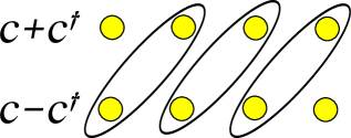
(a)   (b) 

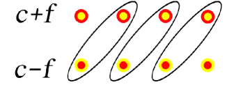
Figure 3: (Color online) (a) Majorana decomposition of Kitaev model; (b) $t=\Delta=V$ limit of the tight binding model (16)

To demonstrate the edge state wave function we can choose $f$ and $c$ hopping to be equal $t=\Delta$, keeping the hybridization a free parameter. The Hamiltonian (16) can be rewritten in the following simple form:

$$H_{(\Delta=t)} = (\Delta+V)\sum_{j,\sigma}(s{{}^{\dagger}}_{j+1\sigma}a_{j\sigma}+\mbox{H.c.})$$ (21)

$$+ (\Delta-V)\sum_{j,\sigma}(s{{}^{\dagger}}_{j-1\sigma}a_{j\sigma}+{\rm H.c}),$$ (22)

where

$$a_{j\sigma}=(f_{j\sigma}-c_{j\sigma})/\sqrt{2},$$ (23)

$$s_{j\sigma}=(f_{j\sigma}+c_{j\sigma})/\sqrt{2}.$$ (24)

The two terms in Hamiltonian (18) correspond to “right facing” and “left facing” bonds between a chain of “a” and “s” sites. In the particular limit that $\Delta=V$, the Hamiltonian consists entirely of right-facing bonds, as illustrated in Fig. 3b, with edge on the left and right composed of symmetric and antisymmetric combinations of conduction and “f” electrons. Note that at first glance this model breaks inversion symmetry, but in fact there is an additional $U(1)$ gauge invariance for $f$ electrons: the phase of $f$ can be rotated, effectively interchanging between antisymmetric $a_{j}$ and symmetric $s_{j}$ operators.

For all values of $V$ and $\Delta$, the zero-mode $\psi_{0}$ can be found solving $H_{(\Delta=t)}\psi_{0}=0$ with the ansatz

$$\psi_{0}=\sum_{j}v_{j}s_{j}^{\dagger}+u_{j}a^{\dagger}_{j}\\$$ (25)

Solving for $\{u_{j},v_{j}\}$ in case $(V\Delta)>0$ we can find left and right edge solutions. The left-hand edge state is given by

$$\begin{split}&u_{j}=0\\ &v_{j}=\left\{\begin{array}[]{l l}\left({V+\Delta\over V-\Delta}\right)^{(j-1)/2}&\quad\text{odd}\\ 0&\quad\text{even}\end{array}\right.\end{split}$$ (26)

Hence, unless hybridization $V$ or effective hopping $\Delta$ is zero the decay is exponential. The fact that $v_{even}=0$ is due to particle hole transformation: one can show that the zero-mode of bipartite lattice is defined only on one sublattice in a one-dimensional finite chain.

III Mean field solution

We now consider a finite slab of material, examining the departures in $V$ and $\Delta$ which develop in the vicinity of the boundaries a phenomenon we refer to as “Kondo band-bending”. The allowed values of $V_{j}$ and $\Delta_{j}$ are determined by the self-consistency equations

$$\begin{split}&V_{j}=-J_{K}{(j)}\left\langle(c_{j+1,\sigma}-c_{j-1,\sigma})^{\dagger}f_{j,\sigma}\right\rangle,\\ &\Delta_{j}=-J_{H}\left\langle f_{j,\sigma}^{\dagger}f_{j+1,\sigma}\right\rangle,\end{split}$$ (27)

These equations derive from the requirement that the acton is stationary with respect to $V_{j}$ and $\Delta_{j}$ at each site. The phase diagram is determined by the values of $J_{H}$, $J_{K}$ and the edge parameter $\alpha$. To explore the parameter space we carried out a series of a numerical calculations in which we seeded inhomogeneous order parameters $V_{j}$ and $\Delta_{j}$, iterating the self-consistency conditions until a convergent solution was found.

To examine the bulk properties, we began by imposing periodic boundary conditions. Using this procedure, we identified two bulk phases: a Kondo insulator and a metallic valence bond solid. The results of mean field calculations with periodic boundary conditions are presented in Fig. 4. The bulk phase diagram is of course independent of the edge parameter $\alpha$.

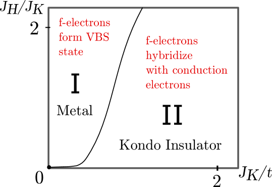
Figure 4: Schematic phase diagram of the bulk ground state contains metallic phase (I) and insulating phase (II). Phase II can be further divided into surface phases depending on the properties of its surface states see Fig. 7.

We proceed with open boundary conditions and examine the nature of the bound states solutions that develop at the ends where mean field parameters depart from the bulk.

III.1 Phase I: Metallic VBS state

In this phase the RVB order parameter $\Delta_{j}$ becomes an alternating function of space, while $V_{j}$ is zero. Consequently, the f-electrons form a valence bond solid (VBS) state, co-existing with the unperturbed conduction sea. Dispersionless “spinon” bands above and below the Fermi energy, as shown in see Fig. 5b. The gap between f-states is provided by the amplitude of $\Delta_{j}$ (justifying the notation) which is in turn equal to $J_{H}/4$. The metallic VBS phase is summarized in Fig. 5a,b.

The metallic phase does not have surface states and behaves the same way for open and closed boundary conditions. We found VBS state to be the lowest energy configuration in the left part of phase diagram as shown in Fig. 4.

Since there are two degenerate configurations of the VBS, one of the important classes of excitation of this state is a domain-wall soliton formed at the interface of the two degenerate vacua. In an isolated VBS, such as the ground-state of the Majumdar Ghosh model, or the Su-Schrieffer-Heeger model, such solitons are spin-1/2 excitations. However, in the 1D Kondo lattice, the Kondo interaction is expected to screen such isolated spins, forming a p-wave Kondo singlet exciton. In the metallic VBS, these solitonic excitons will be gapped excitations. However, as the Kondo coupling grows, at some point the excitons will condense, and at this point the VBS melts, forming a topological Kondo insulator.

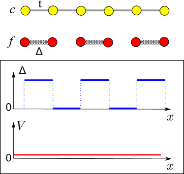
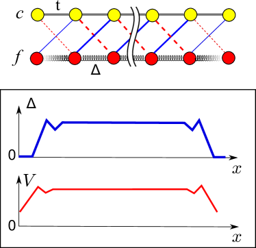
(a)	(c)
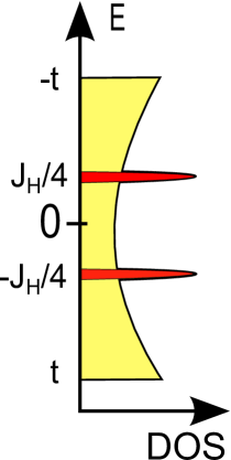
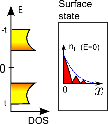
(b)	(d)

Figure 5: Cartoon representation of two distinct phases. Spatial dependence of $V_{j}$ and $\Delta_{j}$ and density of states (DOS) for phase I and II in Fig. 4.Phase I (a and b): Metallic states with suppressed hybridization. It does not support surface states. Phase two (c and d): Kondo topological insulator that support surface states. Inset in d is the profile of a typical surface state decaying into the bulk as a function of distance.

III.2 Phase II: Kondo insulator

In the Kondo insulating phase the hopping $\Delta_{j}$ and $V_{j}$ are both finite in the bulk and generally suppressed at the ends of the chain. This gapped heavy Fermi liquid is stabilized by large Kondo coupling as shown in Fig. 5(c,d). We find that that the Kondo insulating phase exhibits two different kinds of boundary behavior. In the mean field theory, we can characterize these two phases by the fractional conduction electron character $n_{c}\in[0,1]$ of the edge state. The first is adiabatically connected to the “Kitaev point” (see below) in which conduction electrons and composite f-electrons hybridize to form the a surface state with $n_{c}>0$. In the second state, the edge state is a purely localized spin, unhybridized with the conduction electrons ($n_{c}=0$).

III.2.1 “Kitaev” point

For general values of $\{J_{K},J_{H},\alpha\}$ there is no analytic solution. However at the point where $\{J_{K},J_{H},\alpha\}=\{2,4,2\}$ $\Delta_{j}=V_{j}=t$ are constants in space. We now show that at this point each spin component of the mean-field theory corresponds to a two copies of the Kitaev chain, with a single fermionic zero mode at each boundary, as can be seen from the form of the wave function in equation (26). We refer to this particular point in the phase diagram as the ’Kitaev point’.

At this point, following (21), the mean-field Hamiltonian takes the form

$$H_{(\Delta=t)}=2t\sum_{j=1}^{L-1}\sum_{\sigma}(s{{}^{\dagger}}_{j+1\sigma}a_{j\sigma}+\mbox{H.c.}),$$ (28)

where $s_{j\sigma}$ and $a_{j\sigma}$ are the symmetric and antisymmetric combination of states $\frac{1}{\sqrt{2}}(f_{j\sigma}\pm c_{j\sigma})$. This Hamiltonian commutes with the zero modes

$$[H,s_{1\sigma}]=0,\qquad[H,a_{L\sigma}]=0$$ (29)

so for each spin, there is one fermionic zero mode per edge, each involving a hybridized combination of conduction and f-electrons with $n_{c}=\frac{1}{2}$. To see the connection with the Kitaev model, we divide both $s_{j\sigma}$ and $a_{j\sigma}$ into two Majorana fermions as follows,

$$s_{j\sigma}=\frac{1}{\sqrt{2}}(\gamma^{1}_{j\sigma}+i\gamma^{2}_{j\sigma}),\qquad a_{j\sigma}=\frac{1}{\sqrt{2}}(\gamma^{3}_{j\sigma}-i\gamma^{4}_{j\sigma}).$$ (30)

Using (28), the Hamiltonian now splits into two independent components,

$$H_{(\Delta=t)}=-i2t\sum_{j=1}^{L-1}\sum_{\sigma}(\gamma^{1}_{j+1}\gamma^{4}_{j}+\gamma^{2}_{j+1}\gamma^{3}_{j}),$$ (31)

corresponding to a pair of Kitaev chains per spin component. This is natural, because each Kitaev chain has one Majorana zero mode per edge. Since a pair of Majoranas make one normal fermion, this corresponds to one fermionic zero mode per edge.

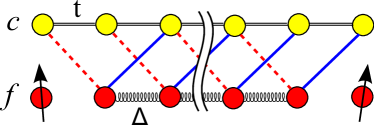
Figure 6: (Color online) Magnetic phase (red color in Fig 7).

III.3 Magnetic Edge state.

In the magnetic edge state, the boundary spins do not undergo the Kondo effect, forming an unhybridized magnetic edge state. If the boundary parameter $\alpha=1$, the Kondo temperature at the boundary is smaller than in the bulk, because the terminal boundary spins have only one nearest neighbor. This means on cooling, that the boundary Kondo interaction is unable to scale to strong coupling before a gap develops in the bulk, leading to an unquenched boundary spin. When $\alpha>1$, the Kondo effect is able to develop at the boundary, occurs at the boundary, provided $J_{K}$ is not at weak coupling. At smaller values of $J_{K}$, the decoupled magnetic phase develops, denoted by the red region in Fig. 7 (a). In this phase, there is no hybridization of the edge state with the bulk conduction electrons ($n_{c}=0$), and the topological edge state disappears.

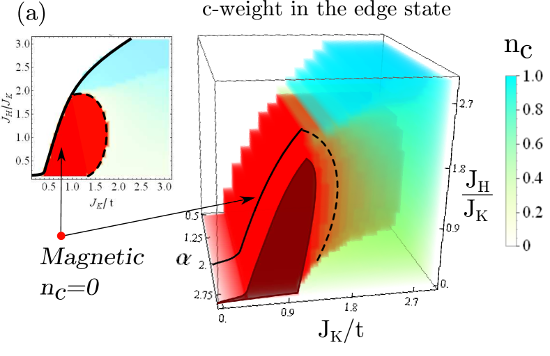
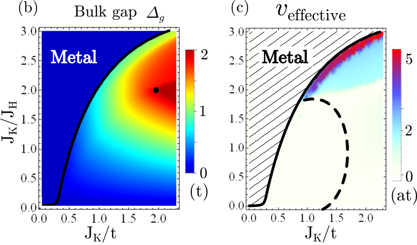
Figure 7: (Color online) The surface phase diagram. With ans addition of renormalized Kondo coupling at the surface $\alpha=J_{K}^{boundary}/J_{K}$. (a) Red color represent pure f-states with no c-electron mixing, $n_{c}=0$. Inset is the cut along $\alpha=2$. (b) (b) is the bulk gap $\Delta_{g}$ in the units of $t$ for $\alpha=2$, identifying the the “Kitaev point” as a black dot. (c) displays the inferred group velocity measured in units of $at$, derived from the measured penetration depth of the edge states using $v=\Delta_{g}\xi$. The mean field calculations were done on a chain of 70 unit cells.

IV Results and Discussion

IV.1 Where are the light surface states?

One of the interesting features of current experiments on the Kondo insulator SmB₆, is that the putative topological surface states seem to involve high-velocity quasiparticles, rather than the heavy, low-velocity particles predicted by current theories. Our mean-field results on the one-dimensional p-wave Kondo chain suggest that this may be because the change in character of the Kondo effect at the boundary leads to edge states with a large conduction electron component.

For a relatively high magnetic interaction, $J_{H}$, the one-dimensional edge states in our mean-field treatment develop majority conduction electron character, forming “light” edge states which penetrate deeply into the bulk.

In a non-interacting topological insulator, the transition to to a topologically trivial phase occurs via a quantum phase transition in which the bulk gap closes. In this case, the penetration penetration depth grows with inverse proportion to the bulk gap $\Delta_{g}$.

$$\xi=v_{F}/\Delta_{g}$$ (32)

However, in the p-wave Kondo chain, the transition to a metallic VBS is a first order transition at which the the bulk gap remains finite. In this case, the rapid growth in the penetration depth of the edge state is associated with an increase in the conduction character, driving an enhanced group-velocity of the edge-states (32). This is a novel and interesting consequence of the response of the Kondo effect to the boundary - “Kondo band-bending”.

To demonstrate this behavior, we have carefully examined the properties of the edge states in our model. The phase diagram showing the evolution in the conduction character of the end states character is shown in Fig. 7a. Within the bulk topological insulator phase, the character of the edge states varies dramatically, ranging from equal f- and c- character at the to to edge states of predominantly conduction electron character near the first order boundary. Fig. 7b shows the dependence of the insulating gap $\Delta_{g}$, showing that it remains finite at the first order phase boundary to the VBS metal.

We can estimate the the effective velocity of the edge states by combining the measured coherence length of the edge state and the bulk gap, according to

$$v_{\hbox{effective}}=\Delta_{g}\xi$$ (33)

This quantity is found to increase dramatically near the first order boundary into the metallic VB state (see 7c), unlike a non-interacting topological insulator, here the increase in $\xi$ is due to a rapidly increasing amount of conduction character in the edge-states, and is not accompanied by a gap closure, so that the effective velocity of the edge states $v_{\hbox{effective}}$ rises considerably.

IV.2 Strong-coupling Ground state wave function

An alternative way to understand a Kondo insulator is through the character of its strong-coupling wavefunction. In an conventional Kondo insulator, the strong coupling ground-state is an array of Kondo singlets. If we write

$$A{{}^{\dagger}}_{j}=\sum_{\sigma=\pm\frac{1}{2}}f{{}^{\dagger}}_{j\sigma}c{{}^{\dagger}}_{j,-\sigma}{\rm sign}(\sigma)$$ (34)

then the strong coupling ground-state of the s-wave Kondo insulator is simply a valence bond solid of Kondo singlets:

$$|KI\rangle = \prod_{j=1}^{L}A{{}^{\dagger}}_{j}|0\rangle.$$ (35)

$$=$$ (36)

where a line denotes a valence bond between a conduction electron (open circle) and a local moment (closed circle).

What then is the corresponding ground-state for the topological Kondo insulator? We can construct variational wavefunctions for the topological Kondo insulator by applying a Gutzwiller projection to the mean-field ground-state. Unlike the s-wave Kondo chain, to preserve the topological ground-state, we need to consider large values for both the Kondo and the Heisenberg coupling. An interesting point to consider is the Kitaev point, where the singlet structure of the mean-field ground-state becomes highly local. By projecting the mean-field ground-state we obtain

$$|TKI\rangle=P_{G}\prod_{j}Z_{j}|0\rangle$$ (37)

where

$$Z_{j}=\sum_{\sigma=\pm\frac{1}{2}}a{{}^{\dagger}}_{j\sigma}s{{}^{\dagger}}_{j+1,-\sigma}{\rm sign\sigma}$$ (38)

with $a{{}^{\dagger}}_{j\sigma}=(f{{}^{\dagger}}_{j\sigma}+c{{}^{\dagger}}_{j\sigma})/sqrt{2}$ and $s{{}^{\dagger}}_{j\sigma}=(f{{}^{\dagger}}_{j\sigma}-c{{}^{\dagger}}_{j\sigma})/sqrt{2}$ as before, whereas $P_{G}=\prod_{j}(n_{f\uparrow}(j)-n_{f\downarrow}(j))^{2}$. Now the valence bond-creation operator

$$Z{{}^{\dagger}}_{j} = \frac{1}{2}\sum_{\sigma}(f{{}^{\dagger}}_{j\sigma}f{{}^{\dagger}}_{j-\sigma}+f{{}^{\dagger}}_{j\sigma}c{{}^{\dagger}}_{j+1,-\sigma}$$ (39)

$$- c{{}^{\dagger}}_{j\sigma}f{{}^{\dagger}}_{j+1,-\sigma}-c{{}^{\dagger}}_{j\sigma}c{{}^{\dagger}}_{j+1,-\sigma}){\rm sign}(\sigma)$$ (40)

is non-local. The projected wavefunction of the TKI now involves a multitude of configurations forming a one-dimensional resonating valence bond (RVB) state between the local moments and conduction electrons. Schematically,

$$|TKI\rangle=\sum\raisebox{-14.45377pt}[0.0pt][0.0pt]{\psfig{width=130.08621pt} },$$ (41)

where we associate a minus sign with left-facing Kondo singlets and conduction electron pairs. In this picture, the edge-states correspond to unpaired spins or conduction electrons at the boundary.

$$|\hbox{edge},\sigma\rangle = P_{G}s{{}^{\dagger}}_{1\sigma}\prod_{j}Z{{}^{\dagger}}_{j}|0\rangle$$ (42)

$$= \sum\raisebox{-14.45377pt}[0.0pt][0.0pt]{\psfig{width=130.08621pt} }$$ (43)

$$+ \sum\ \raisebox{-14.45377pt}[0.0pt][0.0pt]{\psfig{width=130.08621pt} }$$ (44)

At the current time, except in the large $N$ limit, we do not yet know if there is a particular combination of $J_{K}$, $J_{H}$ and hopping $t$ for which the short-range RVB wavefunction is an exact ground-state for the TKI.

IV.3 Further outlook

One of the interesting unsolved questions of is why different methods of growing SmB₆ sometimes suppress the topological surface states. On the one hand, when grown in Al flux, SmB₆ has robust surface states with a low temperature plateau conductivity, whereas the crystals produced with the floating zone method exhibit no plateau conductivity, even though the samples are thought to be cleaner Phelan2014 . Based on our simple one-dimensional model, we speculate that this may because the ordered surface supports localized magnetic moments which in three dimensions, magnetically order. By contrast, for reasons not currently clear, the Al flux grown samples appear to sustain non-magnetic surface states, possibly due to a valence shift at the surface, giving rise to topological surface states. A more detailed understanding of the situation awaits an extension of our current results to a three dimensional model along the lines of Yakovenko2012 . This is work that is currently underway.

Finally, we note that the model we have discussed in this paper can also be engineered in a framework of ultracold atoms where a double well lattice potential is populated with mobile atoms in s and p orbitalsVincent2013 . This may provide a setting for a direct examination of the 1D edge states.

V Acknowledgments

The authors gratefully acknowledge discussions with Onur Erten, Karen Hallberg and Tzen Ong. This work was supported by DOE Grant No. DE-FG02-99ER45790.

References

- (1) F. Haldane, “”Model for a quantum Hall effect without Landau levels: Condensed-matter realization of the parity anomaly”,” Phys. Rev. Lett., vol. 61, no. 18, 1988.
- (2) L. Fu and C. Kane, “Time reversal polarization and a Z2 adiabatic spin pump,” Phys. Rev. B, vol. 74, no. 19, p. 195312, Nov. 2006.
- (3) C. L. Kane and E. J. Mele, “ Topological Order and the Quantum Spin Hall Effect,” Phys. Rev. Lett., vol. 95, no. 14, p. 146802, Sep. 2005.
- (4) C. L. Kane and E. J. Mele, “Quantum Spin Hall Effect in Graphene,” Phys. Rev. Lett., vol. 95, no. 22, p. 226801, Nov. 2005.
- (5) L. Fu, C. Kane, and E. Mele, “Topological Insulators in Three Dimensions,” Phys. Rev. Lett., vol. 98, no. 10, p. 106803, Mar. 2007.
- (6) J. E. Moore, ”The birth of topological insulators.,” Nature, vol. 464, no. 7286, Mar. (2010).
- (7) M. Z. Hasan and C. L. Kane, Reviews of Modern Physics 82, 3045 (2010).
- (8) X. L. Qi and S. C. Zhang, Reviews of Modern Physics 83, 1057 (2011).
- (9) J. Moore and L. Balents, “Topological invariants of time-reversal-invariant band structures,” Phys. Rev. B, vol. 75, no. 12, p. 121306, Mar. 2007.
- (10) R. Roy, “Topological phases and the quantum spin Hall effect in three dimensions,” Phys. Rev. B, vol. 79, no. 19, p. 195322, May 2009.
- (11) X.-L. Qi, T. L. Hughes, and S.-C. Zhang, “Topological field theory of time-reversal invariant insulators,” Phys. Rev. B, vol. 78, no. 19, p. 195424, Nov. 2008.
- (12) Z. Wang, X.-L. Qi, and S.-C. Zhang, “Topological Order Parameters for Interacting Topological Insulators,” Phys. Rev. Lett., vol. 105, no. 25, Dec. 2010.
- (13) M. Dzero, K. Sun, V. Galitski, and P. Coleman, “Topological Kondo Insulators,” Phys. Rev. Lett., vol. 104, no. 10, Mar. 2010.
- (14) H.-C. Jiang, Z. Wang, and L. Balents, “Identifying topological order by entanglement entropy,” Nature Phys., vol. 8, no. 12, pp. 902–905, Nov. 2012.
- (15) R. Nourafkan and G. Kotliar, “Electric polarization in correlated insulators,” Phys. Rev. B, vol. 88, no. 15, p. 155121, Oct. 2013.
- (16) Z. Wang, X.-L. Qi, and S.-C. Zhang, “Topological invariants for interacting topological insulators with inversion symmetry,” Phys. Rev. B, vol. 85, no. 16, p. 165126, Apr. 2012.
- (17) L. Fidkowski and A. Kitaev, “Topological phases of fermions in one dimension”, Phys. Rev. B, vol. 83, no. 7, p. 075103, Feb. 2011.
- (18) C. Wang, A. C. Potter, and T. Senthil, “Classification of interacting electronic topological insulators in three dimensions.”, Science, vol. 343, no. 6171, pp. 629–31, Feb. 2014.
- (19) A. Menth, E. Buehler & T. H. Geballe, Phys. Rev. Lett. 22, 295 (1969).
- (20) S. Wolgast, Ç. Kurdak, K. Sun, J. W. Allen, D.-J. Kim, and Z. Fisk, “Low-temperature surface conduction in the Kondo insulator SmB6”, Phys. Rev. B, Rapid Comm., vol. 88, no. 18, p. 180405, Nov. 2013.
- (21) Zhang, X. et al. “Hybridization, inter-ion correlation, and surface states in the Kondo insulator SmB 6” Phys. Rev. X 3, 011011 (2013).
- (22) D. J. Kim, S. Thomas, T. Grant, J. Botimer, Z. Fisk, and J. Xia, “Surface hall effect and nonlocal transport in SmB₆: evidence for surface conduction.”, Sci. Rep., vol. 3, p. 3150, Jan. (2013).
- (23) G. Li, Z. Xiang, F. Yu, T. Asaba, B. Lawson, P. Cai, C. Tinsman, A. Berkley, S. Wolgast, Y. S. Eo, D. Kim, C. Kurdak, J. W. Allen, K. Sun, X. H. Chen, Y. Y. Wang, Z. Fisk, and L. Li, “Quantum oscillations in Kondo Insulator SmB6,” Jun. 2013.
- (24) M. Neupane, N. Alidoust, S.-Y. Xu, T. Kondo, Y. Ishida, D. J. Kim, C. Liu, I. Belopolski, Y. J. Jo, T.-R. Chang, H.-T. Jeng, T. Durakiewicz, L. Balicas, H. Lin, a Bansil, S. Shin, Z. Fisk, and M. Z. Hasan, “Surface electronic structure of the topological Kondo-insulator candidate correlated electron system SmB6.,” Nature Commun., vol. 4, Dec. 2013.
- (25) N. Xu, X. Shi, P. K. Biswas, C. E. Matt, R. S. Dhaka, Y. Huang, N. C. Plumb, M. Radović, J. H. Dil, E. Pomjakushina, K. Conder, a. Amato, Z. Salman, D. M. Paul, J. Mesot, H. Ding, and M. Shi, “Surface and bulk electronic structure of the strongly correlated system Sm and implications for a topological Kondo insulator”, Phys. Rev. B, vol. 88, no. 12, p. 121102, Sep. 2013.
- (26) J. Jiang, S. Li, T. Zhang, Z. Sun, F. Chen, Z. R. Ye, M. Xu, Q. Q. Ge, S. Y. Tan, X. H. Niu, M. Xia, B. P. Xie, Y. F. Li, X. H. Chen, H. H. Wen, and D. L. Feng, “Observation of possible topological in-gap surface states in the Kondo insulator SmB6 by photoemission.”, Nat. Commun., vol. 4, p. 3010, Dec. 2013.
- (27) E. Frantzeskakis, N. de Jong, B. Zwartsenberg, Y. Huang, Y. Pan, X. Zhang, J. Zhang, F. Zhang, L. Bao, O. Tegus, a. Varykhalov, a. de Visser, and M. Golden, “Kondo Hybridization and the Origin of Metallic States at the (001) Surface of SmB6”, Phys. Rev. X, vol. 3, no. 4, p. 041024, Dec. 2013.
- (28) Lu, F., Zhao, J., Weng, H., Fang, Z., and Dai, X. (2013). “Correlated Topological Insulators with Mixed Valence” Phys. Rev. Lett.,110(9), 096401.
- (29) V. Alexandrov, M. Dzero, and P. Coleman, “Cubic Topological Kondo Insulators”, Phys. Rev. Lett., vol. 111, no. 22, p. 226403, Nov. 2013.
- (30) I. Tamm, Physik. Zeits. Soviet Union 1, 733 (1932).
- (31) W. Shockley, “On the surface states associated with a periodic potential”, Phys. Rev., vol. 56, 317, 1939.
- (32) S. S. Pershoguba and V. M. Yakovenko, “Shockley model description of surface states in topological insulators”, Phys. Rev. B, vol. 86, no. 7, Aug. 2012.
- (33) A. Schnyder, S. Ryu, A. Furusaki, and A. Ludwig, “Classification of topological insulators and superconductors in three spatial dimensions”, Phys. Rev. B, vol. 78, no. 19, Nov. 2008.
- (34) A. Kitaev, “Periodic table for topological insulators and superconductors”, AIP Conf. Proc. 1134, 22, 2009,
- (35) R. King-Smith and D. Vanderbilt, “Theory of polarization of crystalline solids”, Phys. Rev. B, vol 47, 1651-1654 (1993).
- (36) A. Kitaev, “Unpaired Majorana fermions in quantum wires”, Physics-Uspekhi, vol. 131, 2001.
- (37) W. A. Phelan, S. M. Koohpayeh, P. Cottingham, J. W. Freeland, J. C. Leiner, C. L. Broholm, and T. M. McQueen, “Direct link between bulk thermodynamic measurements and surface conduction in SmB6”, Prepr. arXiv:1403.1462, Mar. 2014.
- (38) X. Li, E. Zhao, and W. Vincent Liu, “Topological states in a ladder-like optical lattice containing ultracold atoms in higher orbital bands.”, Nat. Commun., vol. 4, p. 1523, Jan. 2013.