Step Growth and Meandering in a Precursor-Mediated Epitaxy with Anisotropic Attachment Kinetics and Terrace Diffusion

Abstract

Step meandering instability in a Burton-Cabrera-Frank (BCF)-type model for the growth of an isolated, atomically high step on a crystal surface is analyzed. It is assumed that the growth is sustained by the molecular precursors deposition on a terrace and their decomposition into atomic constituents; both processes are explicitly modeled. A strongly nonlinear evolution PDE for the shape of the step is derived in the long-wave limit and without assuming smallness of the amplitude; this equation may be transformed into a convective Cahn-Hilliard-type PDE for the step slope. Meandering is studied as a function of the precursors diffusivity and of the desorption rates of the precursors and adatoms. Several important features are identified, such as: the interrupted coarsening, “facet” bunching, and the lateral drift of the step perturbations (a traveling wave) when the terrace diffusion is anisotropic. The nonlinear drift introduces a disorder into the evolution of a step meander, which results in a pronounced oscillation of the step velocity, meander amplitude and lateral length scale in the steady-state that emerged after the coarsening was interrupted. The mean values of these characteristics are also strongly affected by the drift.

Keywords: epitaxial crystal growth; step flow; meandering instability; molecular precursors; anisotropic diffusion; nonlinear pde model; convective Cahn-Hilliard equation

Mathematics Subject Classification: 35R37; 35Q74; 37N15; 65Z05; 74H10; 74H55

I Introduction

This paper investigates the dynamics of a crystal step (the terrace edge) in the conditions that mimic those in the chemical vapor or beam epitaxy of thin films and its variants (the chemical vapor deposition, metal-organic vapor phase epitaxy, etc.) In the chemical epitaxy the precursor molecules are deposited onto a crystal surface which consists of alternating terraces and steps, undergo diffusion on the terraces and then decompose into the atomic constituents. These adatoms in turn undergo diffusion and then are incorporated into the solid by attachment at the steps.

Despite the abundance of the physico-mathematical models of thwe molecular beam epitaxy (based on a partial differential equations, atomistic, or multi-scale) - whereby there is a single deposited species and no chemical reaction - there is only a handful of models for the epitaxy of multiple atomic species with or without chemical reaction effects. For example, in Refs. CTT ; CTT1 and W the authors study the reaction-diffusion models for the dynamics of a monolayer, where the reaction terms represent the adsorption-desorption and chemical processes, and the diffusion is affected by the nearest-neighbor attractive interactions between the deposited atoms and also by the adatoms-substrate interactions. They find the emergence of self-assembled one-dimensional structures that may precipitate different types of film growth mechanisms. In Refs. CJ1 ; CJ2 an elaborate thermomechanical model for step-flow growth is analyzed, where the diffusing species are coupled through a chemical reaction whereby bulk molecules are crystallized from adatoms attaching to the step edges; the model ensures a configurational force balance at the steps through the generalization of the classical Gibbs-Thomson relation. And in Refs. GMPV ; CPRDKZV a simpler one-dimensional BCFBCF -type model is developed and applied for the analysis of step bunching. In this model the diffusion of adatoms is one-way coupled - through the source term in the diffusion equation - to the diffusion of precursor molecules. The source term originates in decomposition of the precursor, and the corresponding physical boundary conditions are formulated for both species at the step. The latter model has its predecessor in the work by Pimpinelli et al. PCGNT ; PV .

In this paper the model of Refs. GMPV ; CPRDKZV is extended to two dimensions, where the step edge is a plane curve. The goal is to study how the interplay of the precursor and adatom diffusion, desorption, precursor decomposition and adatom attachment to the step influence the step stability and its growth. (Note that desorption of adatoms is neglected in Refs. GMPV ; CPRDKZV .) Step meandering (lateral modulations) is the prominent feature in the experiments GMPV . The meandering can be only studied theoretically using a two-dimensional model.

The first stage in such study is to consider processes such as diffusion on a single (lower) terrace bordering the step (the one-sided model). This greatly simplifies derivations while retaining most of the important physics, and thus we adopt such approach. Besides this simplification, the only other simplification within the framework of BCF-type modeling is the neglect of the adatom diffusion along the step (the line diffusion). On the other hand, we include the rarely considered (due to the complexity of a treatment) diffusion anisotropy on a terrace, both for the precursors and adatoms; the anisotropy of line energy; and the anisotropic attachment kinetics. Thus we consider the full range of anisotropic effects, whose importance was very recently re-emphasized in connection to the island growth on terraces MSL . It was also argued by same authors in Ref. MLKMS that these effects, as well as the coupled dynamics of the precursors and adatoms are important in epitaxial graphene growth on metals. We largely follow these papers in the introduction and notations of the anisotropies. (For a more general treatment of the terrace diffusion anisotropy see Ref. DPKM .)

The derivation relies on a long-wave expansion. There is close physical and mathematical analogy (noted by many authors and also in Ref. MLKMS ) between growth of a crystal into a hypercooled melt and the step growth within the one-sided model. Thus in developing the long-wave evolution PDE for the step profile we pay close attention to the paper by Golovin et al. GDN , who applied this framework to investigate faceting of the growing crystal surface. Our evolution PDE will be a generalization of the one they obtained. (It must be noted that we are concerned only with a weakly anisotropic step energy, in contrast to a strongly anisotropic surface energy in Ref. GDN .)

II Problem formulation

We consider a morphological evolution of an unstable monoatomic step on a crystal surface. A step grows by the flux of adatoms from the lower terrace. The adatoms are the product of the precursors decomposition, and the latter are deposited on a terrace either by condensation from a vapor phase or by a molecular beam. (If the initially straight step is at $z=0$, then the lower terrace is the domain $z>0$.)

The governing equations of the model are the steady-state diffusion equations for the concentrations of the precursors (A) and adatoms (C) on the lower terrace, the mass conservation conditions at the terrace edge $z=h(x,t)$ (the step), the Gibbs-Thomson boundary conditions for the concentrations at the step, and the boundary conditions for the concentrations on the lower terrace far from the step. The problem for the precursors reads GMPV ; CPRDKZV :

$$\nabla\cdot\left(D_{a}\nabla A\right)-\tau_{a}^{-1}A-\chi A=-F,$$ (1)

$$z=h(x,t):\quad\left(D_{a}\nabla A\right)\cdot{\mathbf{n}}=\beta_{a}A,$$

$$z\rightarrow\infty:\quad A=\frac{F}{\tau_{a}^{-1}+\chi}.$$

Here $D_{a}$ is the diffusion tensor, $\tau_{a}^{-1}$ and $\chi$ are the desorption and decomposition rates on a terrace, $F$ is the deposition flux, $\beta_{a}$ is the kinetic coefficient, and ${\mathbf{n}}$ is the unit normal to the step pointing into lower terrace.

The problem for the adatoms reads:

$$\nabla\cdot\left(D_{c}\nabla C\right)-\tau_{c}^{-1}C=-\chi A,$$ (2)

$$z=h(x,t):\quad v_{n}\equiv h_{t}\cos{\theta}=\Omega\left(D_{c}\nabla C\right)\cdot{\mathbf{n}},$$

$$C=C_{eq}\left(1+\frac{\Omega}{k_{B}\bar{T}}\tilde{\beta}_{s}(\theta)\kappa\right)+\tilde{\beta}_{k}(\theta)v_{n},$$ (3)

$$z\rightarrow\infty:\quad C\;\;\mbox{is bounded},$$

where $D_{c}$ is the diffusion tensor, $\tau_{c}^{-1}$ is the desorption rate on a terrace, $v_{n}$ is the step normal velocity, $\Omega$ is the area occupied by an atom, $C_{eq}$ is the equilibrium concentration, $k_{B}\bar{T}$ is Boltzmann’s factor, $\tilde{\beta}_{s}(\theta)$ and $\kappa$ are the step stiffness and the curvature, and $\tilde{\beta}_{k}(\theta)=\beta_{k}(\theta)/(k_{+}\Omega)$ is the kinetic coefficient (here $\beta_{k}(\theta)$ is a dimensionless anisotropy function of the reciprocal attachment coefficient, $1/k_{+}$ MSL ). Also $\theta$ is the angle of ${\mathbf{n}}$ with the $z$-axis. The line diffusion is assumed insignificant and thus this contribution is not included in Eq. (3). The adatom diffusion is coupled to the precursors diffusion through the term $-\chi A$ at the rhs of Eq. (2). This term provides the continuous source of adatoms resulting from decomposition of the precursors; the same term appears with the opposite sign in Eq. (1) CPRDKZV .

For the time being, we write the diffusion tensors as $D_{a}=\bar{D}_{a}\tilde{D}_{a}(\psi),D_{c}=\bar{D}_{c}\tilde{D}_{c}(\psi)$, where $\bar{D}_{a},\bar{D}_{c}$ are the magnitudes, and $\tilde{D}_{a}(\psi),\tilde{D}_{c}(\psi)$ are the dimensionless anisotropies MSL . The length scale is chosen equal to the characteristic distance that a precursor diffuses prior to decomposition: $\ell=\sqrt{\bar{D}_{a}/\chi}$ CPRDKZV . Choosing $\ell^{2}/\bar{D}_{a}=1/\chi$ as the time scale, writing $A=\hat{A}/\Omega,C=C_{eq}+\hat{C}/\Omega$, results in the following dimensionless problems. For the precursors:

$$\nabla\cdot\left(\tilde{D}_{a}\nabla\hat{A}\right)-t_{a}^{-1}\hat{A}=-f,$$ (4)

$$z=h(x,t):\quad\left(\tilde{D}_{a}\nabla\hat{A}\right)\cdot{\mathbf{n}}=\hat{\beta}_{a}\hat{A},$$ (5)

$$z\rightarrow\infty:\quad\hat{A}=t_{a}f.$$ (6)

For the adatoms:

$$\nabla\cdot\left(\tilde{D}_{c}\nabla\hat{C}\right)-t_{c}^{-1}\hat{C}=-\hat{\chi}\hat{A}+g,$$ (7)

$$z=h(x,t):\quad\hat{C}=d_{0}\beta_{s}(\theta)\kappa+\beta_{0}\beta_{k}(\theta)\left(\tilde{D}_{c}\nabla\hat{C}\right)\cdot{\mathbf{n}},$$ (8)

$$z\rightarrow\infty:\quad\hat{C}\;\;\mbox{is bounded}.$$ (9)

After the adatom concentration has been determined from Eqs. (7)-(9), the step profile dynamics is found from

$$h_{t}\cos{\theta}=\bar{D}\left(\tilde{D}_{c}\nabla\hat{C}_{|z=h(x,t)}\right)\cdot{\mathbf{n}},$$ (10)

where ${\mathbf{n}}=\left(-h_{x}\cos{\theta},\cos{\theta}\right)$, and $\cos{\theta}=\left(1+h_{x}^{2}\right)^{-1/2}$. We used the same notations for the dimensionless $x,z,t,h,\kappa,\nabla,v_{n}$. The parameters are: $t_{a}^{-1}=1+1/\chi\tau_{a}$, $t_{c}^{-1}=1/\bar{D}\chi\tau_{c}$, $f=F\Omega/\chi$, $\hat{\beta}_{a}=\beta_{a}\ell/\bar{D}_{a}$, $\hat{\chi}=\chi\ell^{2}/\bar{D}_{c}\equiv 1/\bar{D}$, $g=t_{c}^{-1}\Omega C_{eq}$, $d_{0}=\Omega^{2}\gamma C_{eq}/\left(k_{B}\bar{T}\ell\right)$ (where $\gamma$ is the mean step energy), $\beta_{0}=\bar{D}_{c}/\left(k_{+}\ell\right)$, and $\bar{D}=\bar{D}_{c}/\bar{D}_{a}$. Notice that $\chi\tau_{a}$ and $\bar{D}\chi\tau_{c}$ are the dimensionless reciprocal desorption rates of the precursors and the adatoms, respectively.

The step stiffness and kinetic anisotropies are chosen smooth and periodic MSL :

$$\beta_{s}(\theta)=1+\epsilon_{s,m}\cos{m\theta},\;-1<\epsilon_{s,m}<1,$$

$$\beta_{k}(\theta)=1+\epsilon_{k,m}\cos{(m\theta-m\theta_{0})},\;-1<\epsilon_{k,m}<1.$$

The conditions on the amplitudes $\epsilon_{s,m},\epsilon_{k,m}$ ensure that the anisotropies are positive and thus no orientations are “missing” from the equilibrium and kinetic shapes of the step. (The presence of such orientations usually warrants the inclusion of the regularization term in the Gibbs-Thomson condition (3) GDN ; K .)

Finally, the diffusion tensors have the form MSL

$$D_{a}=\bar{D}_{a}\tilde{D}_{a}(\psi)\equiv\bar{D}_{a}\left(\begin{array}[]{cc}d_{11}(\psi)&\epsilon d_{12}(\psi)\\ \epsilon d_{21}(\psi)&d_{22}(\psi)\\ \end{array}\right),\quad D_{c}=\bar{D}_{c}\tilde{D}_{c}(\psi),$$

where $\tilde{D}_{c}(\psi)=\tilde{D}_{a}(\psi)$, $\epsilon$ is a small positive parameter (see the next Section), $d_{11}=1+\delta\cos{2\psi},d_{12}=d_{21}=\delta\sin{2\psi},d_{22}=1-\delta\cos{2\psi}$, $\delta$ is related to the eigenvalues of the tensor, and $\psi$ is the tensor axes rotation angle. The assumption that the off-diagonal elements of the tensors are O(1) in $\epsilon$ is consistent with the long-wave expansion presented in the next Section. Clearly, we also assumed that the diffusion anisotropy is the same for the precursors and adatoms, and the only difference is the magnitudes of the diffusivities $\bar{D}_{a}$ and $\bar{D}_{c}$. When $\delta=0$, the diffusion is isotropic. When $\delta\neq 0$ and $\psi$ is the root of $\sin{2\psi}=0$, the diffusion is weakly anisotropic; for other $\psi$ values it is strongly anisotropic.

The consideration in this paper will be limited to:

1. The case $\chi^{-1}<\tau_{a}$. This condition means that the time elapsed prior to the precursor decomposition is less than the time elapsed prior to its desorption; otherwise, there is no adatoms on a terrace.

2. The fixed adatom diffusivity $\bar{D}_{c}$. The effects of varying the precursor diffusivity $\bar{D}_{a}$ will be to some degree investigated. Notice that the variations of $\bar{D}_{a}$ and correspondingly, the ratio $\bar{D}$, affect the dimensionless parameters $t_{c}^{-1},\;\hat{\beta}_{a},\;g$ and $d_{0}$.

Complementary to the item 2 in the above list, several important remarks regarding dimensionless parameters in our multi-parametric problem are in order. First, through varying the parameter $t_{a}^{-1}$ in Eq. (4) one can gauge the relative strengths of the precursor’s decomposition and desorption. The limit $t_{a}^{-1}\rightarrow\infty$, or equivalently $\chi\tau_{a}\rightarrow 0$ corresponds to pure desorption (no decomposition). The opposite limit $t_{a}^{-1}\rightarrow 1$, or $\chi\tau_{a}\rightarrow\infty$ corresponds to pure decomposition (no desorption). These limits (as well as any finite variations of $t_{a}^{-1}$) can be achieved either by varying $\tau_{a}$ at fixed $\chi$, or vice versa, by varying $\chi$ at fixed $\tau_{a}$. In the former case $t_{a}^{-1}$ and $t_{a}f$ (the far field precursor concentration) are the only parameters that change values, but in the latter case also $t_{c}^{-1}$, $f$, $\hat{\chi}$ and $g$ change. Similar considerations apply to $t_{c}^{-1}$. Other reasonable choices of the length and time scales also result in the dependencies of several key dimensionless parameters on $\chi,\;\tau_{a},\;\tau_{c}$ and $\bar{D}_{a}$. (See Ref. ZV_arxiv for the in-depth (and complicated) discussion of the characteristic scales involved in the precursor-mediated growth problem.)

We do not make an attempt to fully explore this vast parameter space, rather we choose to demonstrate some key features and trends of the step growth. A detailed parametric study of the step dynamics, in particular the impacts of varying strengths of the kinetic and step energy anisotropies, will be published separately.

III Long-wave expansion

Our analysis begins with the formal long-wave expansion as in Ref. GDN :

$$x = \frac{X}{\epsilon},\;t=T_{0}+\frac{T_{2}}{\epsilon^{2}}+\frac{T_{4}}{\epsilon^{4}}+...,\;A=A_{0}(X,z,T_{0},T_{2},...)+\epsilon^{2}A_{2}(X,z,T_{0},T_{2},...)+...,$$

$$C = C_{0}(X,z,T_{0},T_{2},...)+\epsilon^{2}C_{2}(X,z,T_{0},T_{2},...)+...,$$

where $X$ is the long-scale spatial coordinate, $T_{0}$ is the fast time, $T_{2},T_{4},...$ are the slow time variables and $\epsilon\ll 1$ is the small and dimensionless expansion parameter . Notice that we do not expand the step position $h$, thus $h(X,T_{0},T_{2},...)$ is $O(0)$ in $\epsilon$, meaning that the long-wave evolution equation for the step profile that we will derive is strongly nonlinear and thus it is capable of describing large deformations of the step. This equation therefore differs from weakly nonlinear equations of Kuramoto-Sivashinsky type derived near the instability threshold, see for example Ref. BMV ; SU .

Next, we proceed to derive the solutions to the partially coupled diffusion problems (4)-(6) and (7)-(9) at orders of $\epsilon$ zero, two, and four. The well-posed evolution equation for the step profile emerges after combining contributions at these orders, similar to Ref. GDN . Without the significant loss of generality, we assume $t_{c}\neq t_{a}\Leftrightarrow\alpha_{1}\neq\alpha_{3}$ (see Appendix for the definitions of $\alpha_{1}$ and $\alpha_{3}$). When this assumption does not hold, the solution is way more complicated, since a secular terms must be accounted for in the process of solving the ODEs (in the $z$-variable) for $C_{0}$ and $C_{2}$.

At the zeroth order we obtain:

$$\hat{A}_{0}(z,h) = t_{a}f+\alpha_{2}\mbox{e}^{\alpha_{1}(h-z)},$$ (2)

$$\hat{C}_{0}(z,h) = \alpha_{4}\mbox{e}^{\alpha_{3}(h-z)}+q_{2}\mbox{e}^{\alpha_{1}(h-z)}+q_{1},$$ (3)

$$\bar{D}^{-1}h_{T_{0}} = -d_{22}\left(\alpha_{3}\alpha_{4}+\alpha_{1}q_{2}\right).$$ (4)

Expressions for $\alpha_{1}$ - $\alpha_{4}$, $q_{1}$ and $q_{2}$ in terms of the dimensionless parameters from Section II (and Table 1) are in Appendix. Notice that the step at this order is straight and it translates with a constant velocity.

At the second order the solutions are:

$$\hat{A}_{2}=\left\{\frac{\alpha_{2}}{4\alpha_{1}d_{22}}\left(1+2\alpha_{1}z\right)\left[d_{11}\left(h_{XX}+\alpha_{1}h_{X}^{2}\right)+\left(d_{12}+d_{21}\right)\alpha_{1}h_{X}\right]+s_{2}^{(a)}\left(h,h_{X},h_{X}^{2},h_{XX}\right)\right\}\mbox{e}^{\alpha_{1}(h-z)},$$

$$\hat{C}_{2}=\frac{v\left(h_{X},h_{X}^{2},h_{XX}\right)}{2\alpha_{3}}\left(\frac{1}{2\alpha_{3}}-z\right)\mbox{e}^{\alpha_{3}(h-z)}+\frac{u\left(h_{X},h_{X}^{2},h_{XX}\right)}{\alpha_{1}^{2}-\alpha_{3}^{2}}\mbox{e}^{\alpha_{1}(h-z)}+$$

$$\frac{w\left(h_{X},h_{X}^{2},h_{XX}\right)}{\alpha_{1}^{2}-\alpha_{3}^{2}}\left(\frac{2\alpha_{1}}{\alpha_{1}^{2}-\alpha_{3}^{2}}+z\right)\mbox{e}^{\alpha_{1}(h-z)}+s_{2}^{(c)}\left(h,h_{X},h_{X}^{2},h_{XX}\right)\mbox{e}^{\alpha_{3}(h-z)},$$

$$\bar{D}^{-1}h_{T_{2}}=\left(\alpha_{3}\alpha_{4}+\alpha_{1}q_{2}\right)\left\{\left(d_{21}-d_{11}h_{X}\right)h_{X}+\left(d_{12}+\frac{d_{22}}{2}h_{X}\right)h_{X}\right\}+$$

$$d_{22}\left\{-\alpha_{3}s_{2}^{(c)}+\frac{v}{2}\left(h-\frac{1}{2\alpha_{3}}\right)-\frac{\alpha_{1}u}{\alpha_{1}^{2}-\alpha_{3}^{2}}+\frac{w}{\alpha_{1}^{2}-\alpha_{3}^{2}}\left(1-\alpha_{1}h-\frac{2\alpha_{1}^{2}}{\alpha_{1}^{2}-\alpha_{3}^{2}}\right)\right\}.$$ (5)

The functions $s_{2}^{(a)}$, $s_{2}^{(c)}$, $u,\;v,\;w$ are shown in Appendix. Note that $h$ (but not its derivatives) actually cancels from the rhs of Eq. (5) after these functions are substituted.

Solutions in the fourth order are very cumbersome, but they are necessary since the fourth derivative term, $h_{xxxx}$, is needed to cut-off the short-wavelength instability. (We present only the intermediate compact form of $h_{T_{4}}$ in Appendix.) Next, transferring to the reference frame moving in the $z$-direction with the velocity $h_{T_{0}}$, combining derivatives:

$$h_{t}=\epsilon^{2}h_{T_{2}}+\epsilon^{4}h_{T_{4}},$$ (6)

and introducing the original variable $x$ (which cancels the powers of $\epsilon$ in Eq. (6)) results in the final evolution PDE for the step profile:

$$\bar{D}^{-1}h_{t}=\left(p_{1}^{(2)}+p_{1}^{(4)}\right)h_{xx}+p_{2}^{(2)}h_{x}+p_{3}^{(2)}h_{x}^{2}+p_{4}^{(4)}h_{x}^{3}+p_{5}^{(4)}h_{x}^{4}+p_{6}^{(4)}h_{xx}h_{x}+p_{7}^{(4)}h_{xx}h_{x}^{2}+$$

$$p_{8}^{(4)}h_{xx}^{2}+p_{9}^{(4)}h_{xxx}+p_{10}^{(4)}h_{xxx}h_{x}+p_{11}^{(4)}h_{xxxx},$$ (7)

where the explicit, final forms of the coefficients are presented in the supplementary materials. The superscript (2) or (4) refers to the order of the expansion in which the corresponding term emerges. (The $h_{xx}$ term has the contributions from both the second and fourth orders.)

The primary facts about Eq. (7) are as follows:

1. The linear part of the equation is

   $$\bar{D}^{-1}h_{t}=\left(p_{1}^{(2)}+p_{1}^{(4)}\right)h_{xx}+p_{2}^{(2)}h_{x}+p_{9}^{(4)}h_{xxx}+p_{11}^{(4)}h_{xxxx},$$ (8)

   where $p_{1}^{(2)}+p_{1}^{(4)},p_{11}^{(4)}<0$ in the case of a long-wave instability.

2. When the coefficients of the first and the third derivative terms in Eq. (8) are non-zero, the result is the lateral drift (in the $x$-direction) of step the perturbations with the speed $\bar{D}|p_{2}^{(2)}-p_{9}^{(4)}|$ (the traveling wave solution). The coefficients $p_{2}^{(2)}$ and $p_{9}^{(4)}$ vanish when the off-diagonal elements of the diffusion tensors are zero, that is, $d_{12}(\psi)=d_{21}(\psi)=0$. In other words, the diffusion on the lower terrace must be strongly anisotropic for the emergence of the drift. The drift affects the nonlinear dynamics of the step, as described in Section VI. In addition to $p_{2}^{(2)}$ and $p_{9}^{(4)}$ vanishing when $d_{12}(\psi)=d_{21}(\psi)=0$, also the coefficients $p_{1}^{(4)}$, $p_{4}^{(4)}$, $p_{6}^{(4)}$ vanish in this case. Then the nonlinear PDE (7) simplifies to

   $$\bar{D}^{-1}h_{t}=p_{1}^{(2)}h_{xx}+p_{3}^{(2)}h_{x}^{2}+p_{5}^{(4)}h_{x}^{4}+p_{7}^{(4)}h_{xx}h_{x}^{2}+p_{8}^{(4)}h_{xx}^{2}+p_{10}^{(4)}h_{xxx}h_{x}+p_{11}^{(4)}h_{xxxx}.$$ (9)

   Eq. (9) most closely resembles the Kuramoto-Sivashinsky (KS)-type equation (4.1) from Ref. SU . That equation accounts for weak anisotropy of the line energy, but other anisotropies are not accounted for. Eq. (9) has the same linear terms as the cited equation, and like that equation it contains the nonlinear terms proportional to $h_{x}^{2}$ and $h_{xx}h_{x}^{2}$, where the latter term emerges due to line energy anisotropy. In addition, there is three strongly nonlinear terms $p_{5}^{(4)}h_{x}^{4},\;p_{8}^{(4)}h_{xx}^{2}$ and $p_{10}^{(4)}h_{xxx}h_{x}$ that are due to the assumed large deformation of the step ($h(X,T_{0},T_{2},...)$ is $O(0)$ in $\epsilon$). These terms are not in equation (4.1) of Ref. SU , since step deformations are assumed small in that work.

Eq. (7) can be written in the conservative form for the slope $q\equiv h_{x}$:

$$\bar{D}^{-1}q_{t}=\left[p_{2}^{(2)}q+p_{3}^{(2)}q^{2}+p_{4}^{(4)}q^{3}+p_{5}^{(4)}q^{4}+p_{8}^{(4)}q_{x}^{2}+p_{10}^{(4)}qq_{xx}\right]_{x}+\left[\frac{\partial G}{\partial q}+p_{9}^{(4)}q_{x}+p_{11}^{(4)}q_{xx}\right]_{xx},$$ (10)

where $G(q)$ is the double-well “free energy”:

$$G=-m_{1}q^{2}+m_{2}q^{3}+m_{3}q^{4},\quad m_{1}=-\frac{1}{2}\left(p_{1}^{(2)}+p_{1}^{(4)}\right),\;m_{2}=\frac{p_{6}^{(4)}}{6},\;m_{3}=\frac{p_{7}^{(4)}}{12}.$$

Eq. (10) generalizes the convective Cahn-Hilliard equation (CCHE) (51) from Ref. GDN . It includes the following additional terms: the slope drift terms $p_{2}^{(2)}q_{x}$ and $p_{9}^{(4)}q_{xxx}$, the convective term $p_{4}^{(4)}\left(q^{3}\right)_{x}$, and the higher-order convective terms $p_{8}^{(4)}\left(q_{x}^{2}\right)_{x}$, $p_{10}^{(4)}\left(qq_{xx}\right)_{x}$. The coefficients $p_{i}^{(j)}$ of these terms vanish when $d_{12}=d_{21}=\beta_{0}=0$, that is, the terrace diffusion is isotropic and there is no kinetic contribution in the Gibbs-Thomson condition (3).

It follows from Eq. (7) that the step is linearly unstable with respect to the long-wave perturbations having wavenumbers $k<k_{c}=\sqrt{\left(p_{1}^{(2)}+p_{1}^{(4)}\right)/p_{11}^{(4)}}$. The maximum perturbation growth rate is attained at $k=k_{max}=k_{c}/\sqrt{2}$; correspondingly, $\lambda_{max}=2\pi/k_{max}$.

IV Limited study of parametric dependencies

For the typical values of the dimensional parameters Gillet , the translation velocity $h_{T_{0}}$ of the straight step (Eq. (4)) is positive, i.e. the step grows, when $q_{1}>0$. (Notice that $q_{1}$ is a value of $\hat{C}_{0}$ at $z\rightarrow\infty$, see Eq. (3), and because $\hat{C}_{2},\hat{C}_{4},...$ are zero at $z\rightarrow\infty$, the total dimensional concentration there is $C_{eq}+\Omega q_{1}$.) Also, the condition $h_{T_{0}}>0$ is equivalent to above the threshold precursors concentration at $z\rightarrow\infty$. In dimensional units:

$$z\rightarrow\infty:A_{0}=F/\left(\tau_{a}^{-1}+\chi\right)>C_{eq}/(\tau_{c}\chi).$$

$t_{a}^{-1}$	$f$	$\hat{\beta}_{a}$	$t_{c}^{-1}$	$\hat{\chi}$	$g$	$d_{0}$	$\beta_{0}$	$\epsilon_{s,m}$	$\epsilon_{k,m}$	$\theta_{0}$	$\delta$	$m$	$\psi$
1.02	0.02	180.5	0.5	1	0.004	0.0004	0.005	0.001	0.08	$0$	0, 1/3	6	$\pi/6$

Table 1: The base set of the dimensionless parameters values. These values correspond to $\chi\tau_{a}=50$, $\chi\tau_{c}=2$, and $\bar{D}=1$.

Figures 1(a,b,c) show $k_{c}$ in the isotropic case ($\delta=0$) vs. $\chi\tau_{a}$, $\chi\tau_{c}$, and $\bar{D}$. In Fig. 1(a), as the dimensionless adatom desorption rate decreases ($\tau_{c}$ increases at fixed $\bar{D}$ and $\chi$) the step becomes more stable, but when the dimensionless precursor desorption rate decreases ($\tau_{a}$ increases at fixed $\chi$), the stability does not change appreciably. The former echoes the single-species case. In Fig. 1(b), as the dimensionless precursor desorption rate decreases ($\chi$ increases at fixed $\tau_{a}$) the step becomes more stable, the faster so the smaller is the dimensionless adatom desorption rate (larger $\bar{D}\chi\tau_{c}$). And in Fig. 1(c), as $\bar{D}$ increases (precursor diffusivity $D_{a}$ decreases) the step becomes more stable. Combined, the dependencies of $k_{c}$ on $\chi\tau_{a}$ shown in Figs. 1(a,b) demonstrate that the precursor decomposition impacts step stability significantly more than desorption.

Figure 1: (a) Solid line: $k_{c}$ vs. $\chi\tau_{c}$, where $\chi$ and $\tau_{a}$ are fixed, such that $\chi\tau_{a}=50$; $\bar{D}=1$. (The latter is equivalent to the constant precursor desorption rate $\left(\chi\tau_{a}\right)^{-1}=0.02$ and the combined precursors desorption and decomposition rate $t_{a}^{-1}=1.02$.) Dashed line: $k_{c}$ vs. $\chi\tau_{a}$, where $\chi$ and $\tau_{c}$ are fixed, such that $\chi\tau_{c}=2$; $\bar{D}=1$ $(\equiv t_{c}^{-1}=1/2)$. (b) Solid line: $k_{c}$ vs. $\chi\tau_{a}$, where $\tau_{a}$ is fixed and $\tau_{c}=0.1\tau_{a}$. Dashed line: Same, but $\tau_{c}=\tau_{a}$. Dash-dot line: Same, but $\tau_{c}=10\tau_{a}$. $\bar{D}=1$. (c) $k_{c}$ vs. $\bar{D}$; $\chi\tau_{a}=50$, $\chi\tau_{c}=2$.

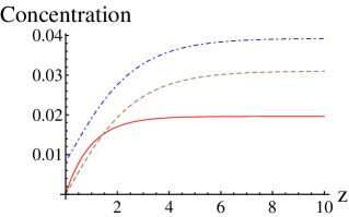
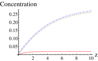
Figure 2: (Color online.) The concentration profiles. Solid line: $\hat{A}_{0}$, dashed line: $\hat{C}_{0}$, dash-dotted line: $\Omega C_{eq}+\hat{C}_{0}$. (a) $\chi\tau_{a}=50$, $\chi\tau_{c}=2$, $\bar{D}=1$; (b) $\chi\tau_{a}=50$, $\chi\tau_{c}=15$, $\bar{D}=1$.

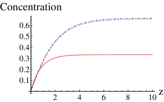
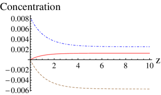
Figure 3: (Color online.) The concentration profiles. (a) $\chi\tau_{a}=2$, $\chi\tau_{c}=2$, $\bar{D}=1$; (b) $\chi\tau_{a}=140$, $\chi\tau_{c}=2$, $\bar{D}=1$. The lines have same meaning as in Fig. 2.

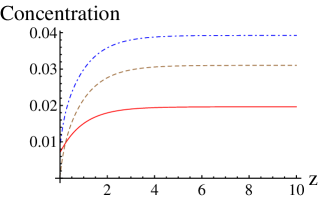
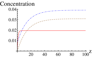
Figure 4: (Color online.) The concentration profiles. (a) $\chi\tau_{a}=50$, $\chi\tau_{c}=2$, $\bar{D}=0.01$; (b) $\chi\tau_{a}=50$, $\chi\tau_{c}=2$, $\bar{D}=100$. The lines have same meaning as in Fig. 2.

Figures 2-4 show the zeroth-order concentration profiles (Eqs. (2) and (3), where we set $h=0$; thus in these figures the step is at $z=0$). The adatom concentration on the terrace increases roughly linear with the increase of $\chi\tau_{c}$ (with $\chi\tau_{a}$ fixed), while the precursors concentration does not change appreciably (Figures 2(a,b)); this is expected, since $\chi\tau_{c}$ is the reciprocal dimensionless desorption rate of the adatoms. When instead $\chi\tau_{c}$ is fixed but $\chi\tau_{a}$ increases, both concentrations decrease (Figures 3(a), 2(a), 3(b)); Fig. 3(b) reflects the situation when the step growth is replaced by evaporation. When $\chi\tau_{a}$ and $\chi\tau_{c}$ are fixed and $\bar{D}$ increases, the precursor and adatom concentrations are constant (Figures 4(a), 2(a), 4(b)) - because the desorption rate $t_{a}^{-1}$ and the flux $f$ in Eq. (4) do not depend on $\bar{D}$, and all of the $t_{c}^{-1},\;\hat{\chi}$ and $g$ in Eq. (7) decrease linearly when $\bar{D}$ increases. Thus one concludes that varying the precursor diffusivity $\bar{D}_{a}$ has no effect on the far-field concentrations on the terrace (see the remark in the end of Section II on the connection of $\bar{D}$ to $\bar{D}_{a}$), but it may strongly affect the step dynamics since the parameters at the step, $\hat{\beta}_{a}$ and $d_{0}$, are $\bar{D}_{a}$-dependent. In fact, this is confirmed by computations, see Sec. V.

In Sections V and VI we describe the computations of the step dynamics. The initial condition for the computations is a random, small-amplitude perturbation of the step profile $h(x,0)=1$ on the domain $0\leq x\leq 30\lambda_{max}$, with the periodic boundary conditions.

V Isotropic dynamics ($\delta=0\Leftrightarrow d_{11}=d_{22}=1,d_{12}=d_{21}=0$)

In this Section the computations of Eq. (9) are described.

For all parameters values, evolution of the step profile from the random initial condition on the large domain proceeds through coarsening, until it stops and a steady-state profile emerges. This scenario is usually termed the interrupted coarsening. It was argued in Refs. PM1 ; PM2 that the signature of uninterrupted coarsening is the positivity of $dA/d\lambda$ for all $\lambda$, where $A$ is the steady-state profile amplitude and $\lambda$ is profile wavelength, given that the initial condition is one (unstable) wavelength of the small-amplitude cosine (or sine) curve on the periodic domain. Indeed, from Fig. 5 it is clear that this condition does not hold.

Figure 5: The profile amplitude vs. its wavelength, in the steady-state. Starting from a small-amplitude, single-wavelength cosine curve on a periodic domain, its evolution was computed until the steady-state cosine curve-like profile emerged. $\chi\tau_{a}=50$, $\chi\tau_{c}=2$, $\bar{D}=100$.

The steady-state step profiles are noticed to be of two types, shown in Figures 6 and 7. The first type is the familiar, regular hill-and-valley structure, which may be also described as the periodic faceted structure. (We use the term “facet” loosely; in fact, the curvature is nowhere zero. Recall that the step energy $\gamma(\theta)$ is a smooth and differentiable function for all step orientations, and the step stiffness $\beta_{s}(\theta)>0$ for all $\theta$.) The second type resulted for large $\bar{D}$ (small $\bar{D}_{a}$), and it consists of the facets bunches. For the first type, Fig. 6(a) shows the steady-state step profile, and Fig. 6(b) shows the corresponding profile slope. It can be seen that the profile is asymmetric, with minimas (valleys) being more pointed than the maximas (hills). The second type steady-state step profile is shown in Fig. 7. Here all facets in the periodic computational domain are separated into bunches, with a clear boundary between them. Such unusual bunching (which to our knowledge has not been previously reported) is attributed to the cumulative effect of the increased precursor decomposition rate at the step, $\hat{\beta}_{a}$ (Eq. (5)), larger adatom concentration at the step through the increased value of $d_{0}$ (Eq. (8)), and larger step velocity (Eq. (10)). These values differ by one to two orders of magnitude from the corresponding values in the $\bar{D}=1$ case shown in Fig. 6 and Table 1.

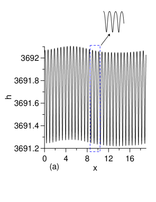
Figure 6: (Color online.) (a) The steady-state step profile. (b) The slope of the steady-state profile (zoom on the interval $9\leq x\leq 11$, corresponding to inset in panel (a)). $\chi\tau_{a}=50$, $\chi\tau_{c}=2$, $\bar{D}=1$.

Figure 7: The steady-state step profile. $\chi\tau_{a}=50$, $\chi\tau_{c}=2$, $\bar{D}=100$.

Fig. 8(a) shows the approach of the characteristic lateral length scale of the profile and the step velocity to the steady-state values. The length scale, $L_{x}$, is defined as the ratio of the computational domain length ($30\lambda_{max}$) to the number of valleys. Fig. 8(b) shows the profile amplitude. The steady state emerges at $t=4000\Leftrightarrow 600$ time units. (This computation was carried up to $t=3.3\times 10^{4}\Leftrightarrow 5\times 10^{3}$ time units, with no change in steady-state values of $L_{x}$, velocity and amplitude.)

In Figures 9(a,b) the steady-state values of the length scale and velocity are plotted vs. $\chi\tau_{a}$ and $\bar{D}$.

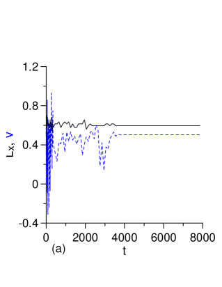
Figure 8: (Color online.) (a) The length scale of the hill-and-valley structure, $L_{x}$ (solid line) and the step velocity (dashed line) vs. $t$. (b) The amplitude of the hill-and-valley structure vs. $t$. Parameters as in Fig. 6.

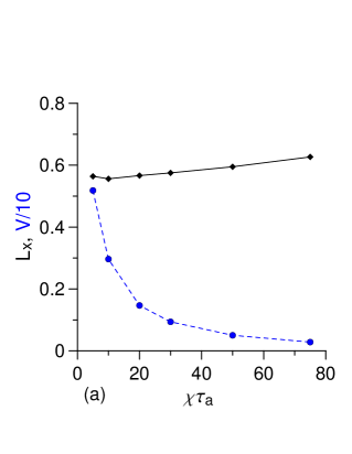
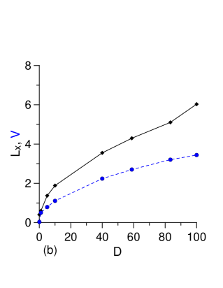
Figure 9: (Color online.) The steady-state length scale of the hill-and-valley structure, $L_{x}$ (diamonds) and the step velocity (circles). (a) Vs. $\chi\tau_{a}$, where $\chi$ and $\tau_{c}$ are fixed, such that $\chi\tau_{c}=2$; $\bar{D}=1$. (b) Vs. $\bar{D}$; $\chi\tau_{a}=50$, $\chi\tau_{c}=2$. The curves are only the guides for the eye.

VI Strongly anisotropic dynamics ($\delta=1/3,\psi=\pi/6\Leftrightarrow d_{11}=7/6,d_{22}=5/6,d_{12}=d_{21}=1/2\sqrt{3}$)

Fig. 10 shows some step profiles for $\theta_{0}=0$ and other parameters as in Fig. 6, computed using Eq. (7). Clearly, there is disorder, and also there is no highly regular steady-state in the form of a hill-and-valley structure as in Fig. 6 - the growth as shown in Fig. 10 continues in the same fashion indefinitely (we computed until $t=2.9\times 10^{4}$). The disorder is due to a nonlinear traveling wave along the step, triggered and sustained by the $h_{x}$, $h_{xxx}$, $h_{x}^{3}$, and $h_{xx}h_{x}$ terms in the evolution Eq. (7). The length scale, velocity and amplitude are shown in Fig. 11. These quantities oscillate around the well-defined mean values, with rather large amplitudes (for instance, the step velocity takes on negative values at some times, i.e. the step locally retracts). Also the mean values of the length scale, velocity, and amplitude themselves are affected by the terrace diffusion anisotropy: both the mean length scale and the amplitude are significantly larger than the steady-state, “isotropic” values in Figures 8(a,b), and the mean velocity is smaller.

Figure 10: Step growth at the strong anisotropy of the terrace diffusion. $\chi\tau_{a}=50$, $\chi\tau_{c}=2$, $\bar{D}=1$. The bottom profile corresponds to $t=80$, the top one to $t=320$.

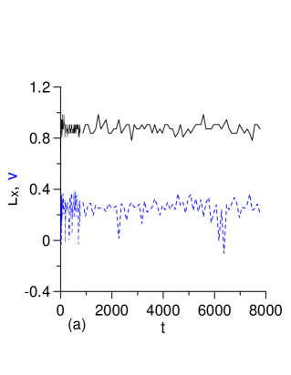
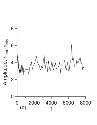
Figure 11: (Color online.) (a) The length scale of step modulations, $L_{x}$ (solid line) and the step velocity (dashed line) from the computation of step growth shown in Fig. 10. (b) The step profile amplitude.

VII Conclusions

The model describing the meandering and growth in the course of a precursor-mediated epitaxy of an isolated, atomically high step on a surface of a thin film has been analyzed. A strongly nonlinear evolution PDE for the amplitude of the meander is derived in the long-wave limit and without assuming smallness of the amplitude; this equation may be transformed into a convective Cahn-Hilliard-type PDE for the meander slope. Computed solutions display an interrupted coarsening and the lateral drift of the meander (a traveling wave), which affect the important and experimentally measurable parameters, such as the amplitude and velocity. Impacts of the varying precursor diffusivity and the desorption rates of the precursors and adatoms on the meander evolution are studied.

In a MOVPE experiments, a step meandering features prominently GMPV . The interrupted coarsening and drift have been described previously by Danker et al. DPKM ; DPKM1 and Hauber et al. HV in the context of models for MBE film growth, where there is a single diffusing species (the adatoms). These effects were attributed either to the anisotropy of the line stiffness, or to the terrace diffusion anisotropy. It was noticed, for instance, that the terrace diffusion anisotropy leads to the tilt of the meander DPKM however, in detail such evolution was not studied. In our Eq. (7) the drift is explicit, its direction is apparent, and its speed is the simple expression, unlike in the evolution equations derived in Refs. DPKM ; DPKM1 .

Without the terrace diffusion anisotropy, the step profiles computed from our local PDE are similar to those in Ref. HV ; the latter profiles were computed using the full free-boundary problem. The profiles also resemble the smoothed versions of the profiles emerging from the analysis of another local PDE, the conserved Kuramoto-Sivashinsky (CKS) equation FV ; GTPB . The latter PDE is derived in Ref. FV also with the accounting for the terrace diffusion anisotropy. The connection of these two models deserves, in our view, some exploration in the future.

The computation of the islands growth in the course of MBE and accounting for a full range of the anisotropic effects was done recently in Refs. MSL ; MLKMS using a phase-field model. It is worth noting that we incorporated all such anisotropic effects into a single, closed-form evolution equation that can be simplified to fit the MBE setup (by employing the obvious and straightforward recalculations stemming from the omission of the precursors from the model).

Appendix A Various dimensionless parameters and functions that appear in the solution expressions presented in section III

$$\alpha_{1}=\sqrt{\frac{t_{a}^{-1}}{d_{22}}},\;\alpha_{2}=\frac{-\hat{\beta}_{a}t_{a}f}{\hat{\beta}_{a}+\alpha_{1}d_{22}},\;\alpha_{3}=\sqrt{\frac{t_{c}^{-1}}{d_{22}}},\;\alpha_{4}=\frac{-q_{1}-q_{2}\left(1+\alpha_{1}\beta_{0}\left(1+\Upsilon_{k,m}\right)d_{22}\right)}{1+\alpha_{3}\beta_{0}\left(1+\Upsilon_{k,m}\right)d_{22}},$$

$$\Upsilon_{k,m}=\epsilon_{k,m}\cos{m\theta_{0}},\;q_{1}=\frac{\hat{\chi}t_{a}f-g}{t_{c}^{-1}},\;q_{2}=\frac{\hat{\chi}\alpha_{2}}{t_{c}^{-1}-\alpha_{1}^{2}d_{22}},$$

$$s_{2}^{(a)}=\left[\alpha_{1}\alpha_{2}h_{x}\left(d_{21}+d_{12}-d_{11}h_{x}+\frac{d_{22}}{2}h_{x}\right)-\right.\left\{\frac{\alpha_{2}}{4}\left(2\alpha_{1}h-1\right)+\frac{\hat{\chi}\alpha_{2}}{4\alpha_{1}d_{22}}\left(2\alpha_{1}h+1\right)\right\}\times$$

$$\left.\left\{d_{11}\left(h_{xx}+\alpha_{1}h_{x}^{2}\right)+\left(d_{12}+d_{21}\right)\alpha_{1}h_{x}\right\}\right]\frac{1}{\hat{\chi}+\alpha_{1}d_{22}},$$

$$u=\frac{1}{d_{22}}\left[-\alpha_{1}d_{11}q_{2}\left(\alpha_{1}h_{x}^{2}+h_{xx}\right)+\alpha_{1}^{2}q_{2}\left(d_{12}+d_{21}\right)h_{x}-\right.$$

$$\left.\frac{\alpha_{2}\hat{\chi}}{4\alpha_{1}d_{22}}\left\{d_{11}\left(\alpha_{1}h_{x}^{2}+h_{xx}\right)+\alpha_{1}\left(d_{12}+d_{21}\right)h_{x}\right\}-\hat{\chi}s_{2}^{(a)}\right],$$

$$v=\frac{1}{d_{22}}\left[\alpha_{3}\alpha_{4}d_{11}\left(\alpha_{3}h_{x}^{2}+h_{xx}\right)+\alpha_{3}^{2}\alpha_{4}\left(d_{12}+d_{21}\right)h_{x}\right],\;w=\frac{-\alpha_{2}\hat{\chi}}{2d_{22}^{2}}\left[d_{11}\left(\alpha_{1}h_{x}^{2}+h_{xx}\right)+\alpha_{1}\left(d_{12}+d_{21}\right)h_{x}\right],$$

$$s_{2}^{(c)}=\frac{1}{1+\alpha_{3}\beta_{0}\left(1+\Upsilon_{k,m}\right)d_{22}}\left(-d_{0}\left(1+\epsilon_{s,m}\right)h_{xx}+\left(1+\Upsilon_{k,m}\right)\beta_{0}\left(\left(d_{12}+d_{21}\right)h_{x}+\left(-d_{11}+\frac{d_{22}}{2}\right)h_{x}^{2}\right)\times\right.$$

$$\left(\alpha_{3}\alpha_{4}+\alpha_{1}q_{2}\right)+\Upsilon_{k,m}\beta_{0}d_{22}h_{x}^{2}\left(\alpha_{3}\alpha_{4}+\alpha_{1}q_{2}\right)r_{1,m}-\frac{u}{\alpha_{1}^{2}-\alpha_{3}^{2}}+\frac{v}{4\alpha_{3}^{2}}+\frac{hv}{2\alpha_{3}}-\frac{2\alpha_{1}w}{\left(\alpha_{1}^{2}-\alpha_{3}^{2}\right)^{2}}-\frac{hw}{\alpha_{1}^{2}-\alpha_{3}^{2}}+$$

$$\left(1+\Upsilon_{k,m}\right)\beta_{0}d_{22}\left(-\frac{\alpha_{1}u}{\alpha_{1}^{2}-\alpha_{3}^{2}}+\frac{1}{2}\left(h-\frac{1}{2\alpha_{3}}\right)v+\left.\frac{\left(1-\frac{2\alpha_{1}^{2}}{\alpha_{1}^{2}-\alpha_{3}^{2}}-\alpha_{1}h\right)w}{\alpha_{1}^{2}-\alpha_{3}^{2}}\right)\right),$$

$$r_{1,m}=8,\;\mbox{if}\;m=4;\quad 18,\;\mbox{if}\;m=6,$$

$$h_{T_{4}}=\frac{h_{X}^{2}}{2}h_{T_{2}}+\bar{D}\left[\beta_{0}\left(1+\Upsilon_{k,m}\right)\left\{d_{21}\hat{C}_{2X}+\left(d_{11}h_{X}-d_{21}\right)\left(\frac{h_{X}^{2}}{2}\hat{C}_{0X}-\hat{C}_{2X}\right)+\right.\right.$$

$$\frac{h_{X}^{3}}{2}\left(\frac{3h_{X}}{4}d_{22}+d_{12}\right)\hat{C}_{0z}-h_{X}\left(\frac{h_{X}}{2}d_{22}+d_{12}\right)\hat{C}_{2z}+$$

$$\left.d_{22}\hat{C}_{4z}\right\}-\beta_{0}\Upsilon_{k,m}r_{1,m}h_{X}^{2}\left\{\left(-d_{11}h_{X}+d_{21}\right)\hat{C}_{0X}-\right.$$

$$\left.\left.h_{X}\left(\frac{h_{X}}{2}d_{22}+d_{12}\right)\hat{C}_{0z}+d_{22}\hat{C}_{2z}\right\}+\beta_{0}\Upsilon_{k,m}r_{2,m}h_{X}^{4}d_{22}\hat{C}_{0z}\right],$$ (1)

$$r_{2,m}=16,\;\mbox{if}\;m=4;\quad 66,\;\mbox{if}\;m=6.$$

In Eq. (1) the derivatives of concentrations are understood to be evaluated at the step $z=h$.

References

- (1) M.G. Clerc, E. Tirapegui, M. Trejo. Pattern Formation and Localized Structures in Reaction-Diffusion Systems with Non-Fickian Transport. Phys. Rev. Lett., 97 (2006), 176102.
- (2) M.G. Clerc, E. Tirapegui, M. Trejo. Pattern formation and localized structures in monoatomic layer deposition. Eur. Phys. J., 146 (2007), 407.
- (3) D. Walgraef. Self-organization and nanostructure formation in chemical vapor deposition. Phys. Rev. E, 88 (2013), 042405.
- (4) P. Cermelli, M. Jabbour. Multispecies epitaxial growth on vicinal surfaces with chemical reactions and diffusion. Proc. R. Soc. A, 461 (2005), 3483.
- (5) P. Cermelli, M. Jabbour. Step bunching during the epitaxial growth of a generic binary-compound thin film. J. Mech. Phys. Solids, 58 (2010), 810.
- (6) A. Gocalinska, M. Manganaro, E. Pelucchi, D. D. Vvedensky. Surface organization of homoepitaxial InP films grown by metalorganic vapor-phase epitaxy. Phys. Rev. B, 86 (2012), 165307.
- (7) A.L.-S. Chua, E. Pelucchi, A. Rudra, B. Dwir, E. Kapon, A. Zangwill, D.D. Vvedensky. Theory and experiment of step bunching on misoriented GaAs(001) during metalorganic vapor-phase epitaxy. Appl. Phys. Lett., 92 (2008), 0113117.
- (8) W.K. Burton, N. Cabrera, F.C. Frank. The growth of crystals and the equilibrium structure of their surfaces. Philos. Trans. R. Soc. London, Ser. A, 243 (1951), 299.
- (9) A. Pimpinelli, R. Cadoret, E. Gil-Lafon, J. Napierala, A. Trassoudaine. Two-particle surface diffusion-reaction models of vapour-phase epitaxial growth on vicinal surfaces. J. Cryst. Growth, 258 (2003), 1.
- (10) A. Pimpinelli, A. Videcoq. Novel mechanism for the onset of morphological instabilities during chemical vapour epitaxial growth. Surf. Sci. Lett., 445 (2003), L23.
- (11) E. Meca, V.B. Shenoy, J. Lowengrub. Phase-field modeling of two-dimensional crystal growth with anisotropic diffusion. Phys. Rev. E, 88 (2013), 052409.
- (12) E. Meca, J. Lowengrub, H. Kim, C. Mattevi, V.B. Shenoy. Epitaxial graphene growth and shape dynamics on copper: phase-field modeling and experiments. Nano Lett., 13 (2013), 5692.
- (13) G. Danker, O. Pierre-Louis, K. Kassner, C. Misbah. Peculiar Effects of Anisotropic Diffusion on Dynamics of Vicinal Surfaces. Phys. Rev. Lett., 93 (2004), 185504.
- (14) A.A. Golovin, S.H. Davis, A.A. Nepomnyashchy. A convective Cahn-Hillliard model for the formation of facets and corners in crystal growth. Physica D, 122 (1998), 202.
- (15) M. Khenner. A long-wave model for strongly anisotropic growth of a crystal step. Phys. Rev. E, 88 (2013), 022402.
- (16) A. Zangwill, D.D. Vvedensky. Regimes of precursor-mediated epitaxial growth. arXiv: 0712.1289 (2007).
- (17) I. Bena, C. Misbah, A. Valance. Nonlinear evolution of a terrace edge during step-flow growth. Phys. Rev. B, 47 (1993), 7408.
- (18) Y. Saito, M. Uwaha. Anisotropy effect on step morphology described by Kuramoto-Sivashinsky equation. J. Phys. Soc. Jpn., 65 (1996), 3576.
- (19) F. Gillet, O. Pierre-Louis, C. Misbah. Non-linear evolution of step meander during growth of a vicinal surface with no desorption. Eur. Phys. J. B, 18 (2000), 519.
- (20) P. Politi, C. Misbah. When does coarsening occur in the dynamics of one-dimensional fronts ?. Phys. Rev. Lett., 92 (2004), 090601.
- (21) P. Politi, C. Misbah. Nonlinear dynamics in one dimension: A criterion for coarsening and its temporal law. Phys. Rev. E, 73 (2006), 036133.
- (22) G. Danker, O. Pierre-Louis, K. Kassner, C. Misbah. Interrupted coarsening of anisotropic step meander. Phys. Rev. E, 68 (2003), 020601(R).
- (23) T. Frisch, A. Verga. Effect of Step Stiffness and Diffusion Anisotropy on the Meandering of a Growing Vicinal Surface. Phys. Rev. Lett., 96 (2006), 166104.
- (24) M. Guedda, H. Trojette, S. Peponas, M. Benlahsen. Effect of step stiffness and diffusion anisotropy on dynamics of vicinal surfaces: a competing growth process. Phys. Rev. B, 81 (2010), 195436.
- (25) F. Hauber, A. Voigt. Step meandering in epitaxial growth. J. Cryst. Growth, 303 (2007), 80.