Present address: ]HRL Laboratories, LLC, Malibu, CA 90265, USA

Present address: ]Institute for Quantum Computing and Department of Physics and Astronomy, University of Waterloo, Waterloo, Ontario, Canada N2L 3G1

Present address: ]Department of Physics, Zhejiang University, Hangzhou 310027, China

Simulating weak localization using a superconducting quantum circuit

Understanding complex quantum matter presents a central challenge in condensed matter physics. The difficulty lies in the exponential scaling of the Hilbert space with the system size, making solutions intractable for both analytical and conventional numerical methods. As originally envisioned by Richard Feynman, this class of problems can be tackled using controllable quantum simulators Feynman1982 ; Buluta2009 . Despite many efforts, building an quantum emulator capable of solving generic quantum problems remains an outstanding challenge, as this involves controlling a large number of quantum elements Aspuru-Guzik2012 ; Blatt2012 ; Bloch2012 . Here, employing a multi-element superconducting quantum circuit and manipulating a single microwave photon, we demonstrate that we can simulate the weak localization phenomenon observed in mesoscopic systems. By engineering the control sequence in our emulator circuit, we are also able to reproduce the well-known temperature dependence of weak localization. Furthermore, we can use our circuit to continuously tune the level of disorder, a parameter that is not readily accessible in mesoscopic systems. By demonstrating a high level of control and complexity, our experiment shows the potential for superconducting quantum circuits to realize scalable quantum simulators.

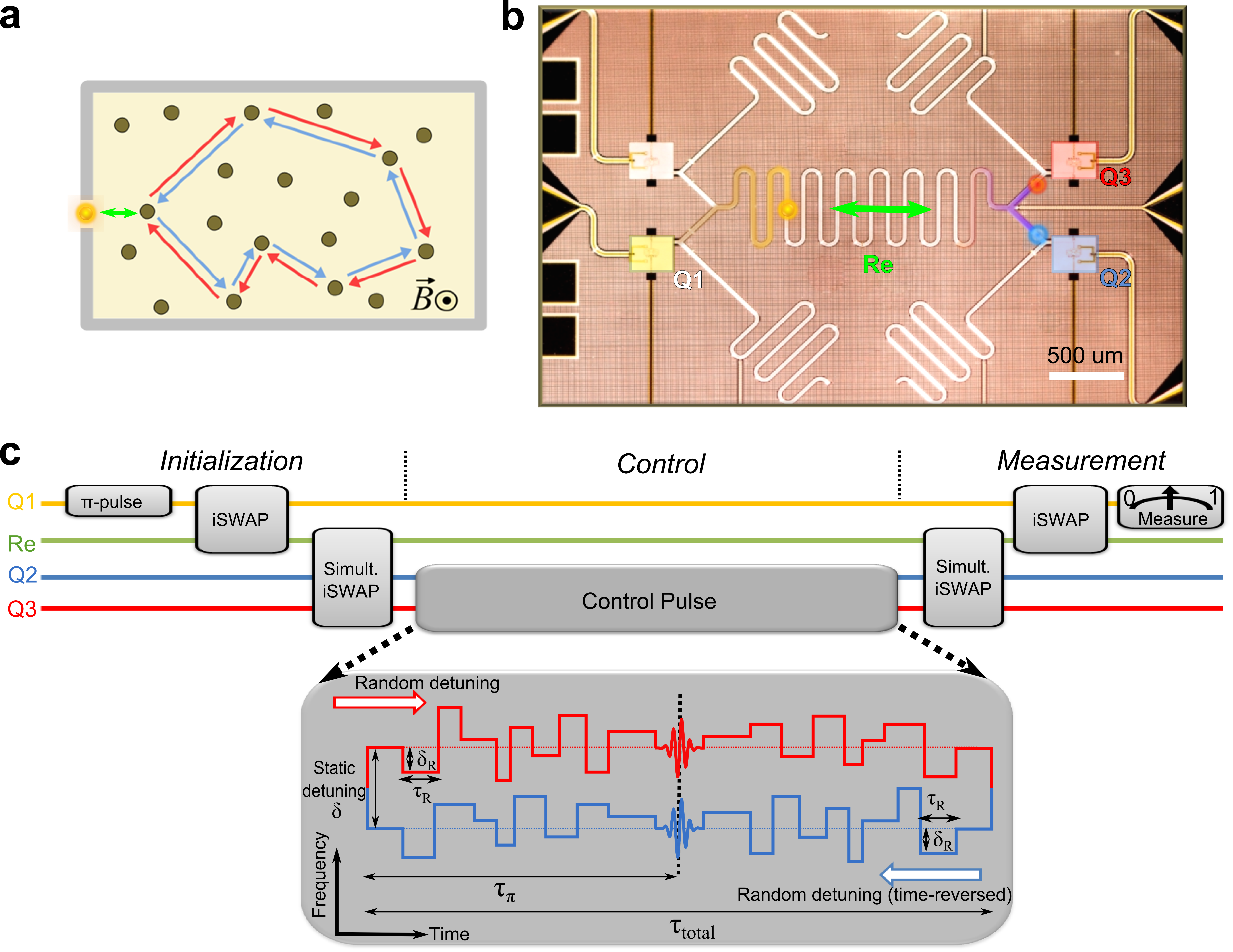
Figure 1: Superconducting quantum circuit implementation of weak localization. a. Schematic illustrating the basic physics of weak localization. The weak localization contribution to electrical resistance is dominated by the interference between closed trajectories traversed in opposite directions, which in the small decoherence limit give an increase in the resistance; here we show one such pair of trajectories. b. Micrograph of the superconducting quantum circuit used to simulate weak localization. A single microwave excitation is generated in qubit $Q1$, distributed between $Q2$ and $Q3$ and the coupling resonator $Re$, then manipulated in the simulation. c. Pulse sequence used to simulate weak localization, decomposed into three steps: Initialization: A $\pi$-pulse creates an excitation in $Q1$ that is then swapped into resonator $Re$ through an iSWAP gate. The simultaneous iSWAP gate then transfers the excitation from $Re$ equally to $Q2$ and $Q3$ through their three-body interaction, creating a state $|\psi\rangle=|Q2\,Q3\,Re\rangle=\frac{1}{\sqrt{2}}(|eg0\rangle+|ge0\rangle)$ that entangles $Q2$ and $Q3$. Control: We apply to $Q2$ a relative static detuning $\delta$, as well as a sequence of random detunings $\delta_{R}$ each lasting for a random time $\tau_{R}$, interspersed with a refocusing $\pi$-pulse spaced in time by $\tau_{\pi}$ to vary the effective coherence time $T_{\varphi^{\text{eff}}}$. We apply the time-reversed sequence to $Q3$. Measurement: A simultaneous iSWAP interferes the states of $Q2$ and $Q3$ in $Re$, and a second iSWAP returns the excitation to $Q1$; the probability for $Q1$ to be in the excited state $|e\rangle$ is then measured.

Superconducting quantum circuits have been used to simulate one- and two-particle problems Neeley2009 ; Raftery2013 , and may be useful for simulation of larger systems Houck2012 . Here, we use a superconducting circuit to simulate the phenomenon of weak localization, a mesoscopic effect that occurs in disordered electronic systems at low temperatures. The challenge in this type of problem is that the mesoscopic observables such as electrical resistance arise from the interference of many scattering trajectories Bergmann1984 , thus apparently requiring a very large emulator. However, we find that we can simulate weak localization using a time-domain ensemble (TDE) approach: We sequentially run through many different circuit parameter sets, each set simulating a different pair of scattering trajectories in the mesoscopic system. By finding a one-to-one correspondence between mesoscopic properties and quantum circuit parameters, we are able to map the spatial complexity of the mesoscopic system onto a set of complex yet manageable quantum control sequences in the time domain.

Electron in mesoscopic system	Photon in quantum circuit
Magnetic field $B$	Static detuning $\delta$
Path area $S$	Total detune pulse time $\tau_{\text{total}}$
Wavevector $\overrightarrow{k}$	Random detuning $\delta_{R}$
Displacement $\overrightarrow{l}$	Pulse duration $\tau$
Coherence length $L_{\varphi}$	Effective coherence time $T_{\varphi^{\text{eff}}}$
Level of disorder	Width of $\tau_{\text{total}}$ distribution $\sigma$
Electrical resistance $R$	Photon return probability $P_{\text{return}}$

Table 1: List of parameters for electron transport in a mesoscopic system, and the corresponding control parameters in a quantum circuit.

Weak localization involves the interference of electron trajectories in a disordered medium Bergmann1984 . The quantum nature of the electron allows it to simultaneously follow multiple trajectories, each with amplitude $A_{n}$ and phase $\phi_{n}$. The probability for the electron to reach a certain point is given by

$$P=\sum_{n}A_{n}^{2}+\sum_{m\neq n}\sum_{n}A_{n}A_{m}\cos(\phi_{n}-\phi_{m}),$$ (1)

where the first term sums over classical probabilities and the second represents quantum interference. The quantum term typically averages to zero, as scattering events randomize the electron wavevector $\overrightarrow{k}$ and displacement $\overrightarrow{l}$ and thus the accumulated phase $\phi=\underset{j}{\sum}\,\overrightarrow{k_{j}}\cdot\overrightarrow{l_{j}}$. A very dominant exception to this occurs in closed trajectories, as these always have a time-reversed counterpart with identical accumulated phase $\phi$ (Fig. 1(a)). These special pairs thus interfere constructively with one another, yielding a probability $P_{\text{return}}=4A^{2}$, twice the classical value. Experimentally, weak localization is identified by applying a magnetic field $\overrightarrow{B}$, which induces an additional static phase shift $\phi_{S}=2\left(2\pi\overrightarrow{B}\cdot\overrightarrow{S}\right)/\Phi_{0}$ for closed trajectories with area $\overrightarrow{S}$. The magnetic field breaks the time-reversal symmetry and the precise constructive interference of the paired closed trajectories. The measured electrical resistance is thus maximum at zero applied field, and falls to the classical resistance value as the magnetic field is increased - a hallmark of weak localization. Reflecting quantum coherence from the electron dynamics, weak localization is most known for its temperature dependence. A elevated temperature increases the inelastic scattering rates, reduces the phase coherence length $L_{\varphi}$, and thus suppresses the magnitude of the weak localization peak at zero magnetic field Bergmann1984 ; Pierre2003 .

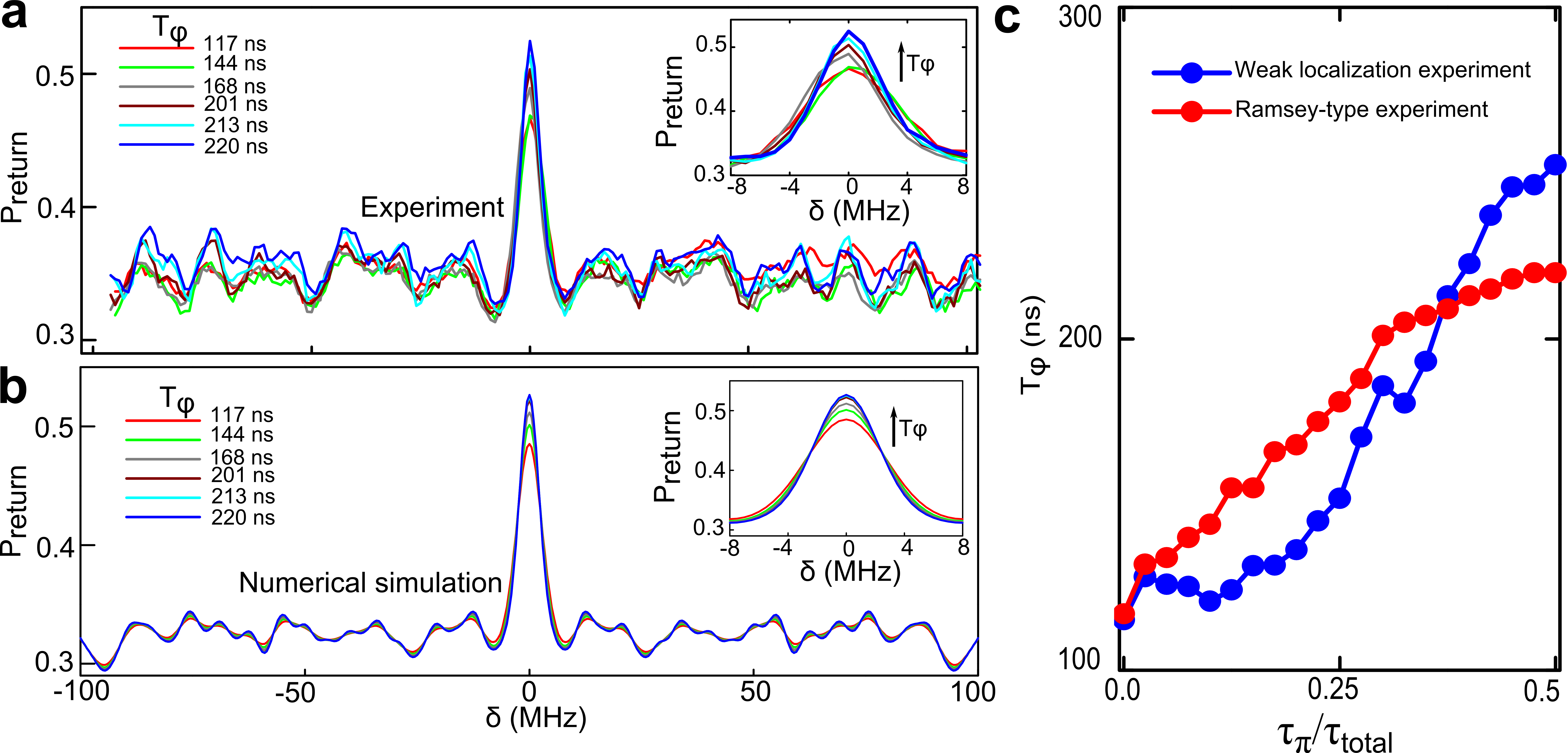
Figure 2: Simulating the temperature dependence of weak localization a. Measured photon return probability $P_{\text{return}}$ as a function of the static detuning $\delta$ (simulating a magnetic field), for six different effective coherence times $T_{\varphi^{\text{eff}}}$. The $P_{\text{return}}$ peak at zero detuning is analogous to the magneto-resistance peak associated with weak localization. Inset shows a magnified view of $P_{\text{return}}$ near $\delta=0$, where we can observe the growth of the $P_{\text{return}}$ peak. This simulates the growth of the magneto-resistance peak when lowering the temperature. b. The photon return probability $P_{\text{return}}$ as a function of $\delta$ obtained through numerical calculations, at the same six different effective coherence time $T_{\varphi^{\text{eff}}}$ as the experiment. c. The effective coherence time $T_{\varphi^{\text{eff}}}$ extracted from the experiments, in comparison to $T_{\varphi^{\text{eff}}}$ directly measured by Ramsey-type experiments, as a function of $\tau_{\pi}/\tau_{\mbox{total}}$.

Replacing the electron with a microwave excitation, we simulate weak localization in a quantum circuit comprising three phase qubits, a readout qubit Q1 and two control qubits Q2 and Q3, symmetrically coupled to a bus resonator Re, as shown in Fig. 1b Lucero2012 . In this configuration, the quantum circuit can be described by the Tavis-Cummings modelTavis1968

$$H=\hbar\omega_{r}a^{+}a+\sum_{i=1}^{3}\hbar\omega_{i}\sigma_{i}^{+}\sigma_{i}^{-}+\sum_{i=1}^{3}\hbar g(a^{+}\sigma_{i}^{-}+a\sigma_{i}^{+}),$$ (2)

where $\omega_{i}$ and $\omega_{r}$ are the frequencies of the qubits and the resonator, respectively, and $g$ is the qubit-resonator coupling strength.

As shown in Fig. 1(c), we start the simulation by splitting the microwave excitation into the two control qubits, analogous to an incoming electron simultaneously traversing two trajectories. This was done by first initializing $Q1$ in $|e\rangle$, swapping the excitation into $Re$ and then applying a simultaneous iSWAP gate Lucero2012 ; Mlynek2012 . By bringing $Q2$ and $Q3$ simultaneously on resonance with $Re$ for an time $t=\pi/(2\sqrt{2}g)$, the simultaneous iSWAP gate transfers the excitation from $Re$ equally to the two control qubits through their three-body interaction, resulting in the desired state $|\psi\rangle=|Q2\,Q3\,Re\rangle=\frac{1}{\sqrt{2}}(|eg0\rangle+|ge0\rangle)$.

To simulate the the diffusion process of the electron in the presence of magnetic field, we then apply a combination of sequences to the control qubits, following the mapping between mesoscopic transport and quantum circuit parameters delineated in Table 1. To mimic the random scattering, we apply a series of random frequency detunings $\delta_{R}^{i}$ to each qubit, each for a random duration $\tau_{i}$ (see the extended pulse sequence in Fig.1(c)), resulting in a dynamic phase $\varphi_{R}=\underset{i}{\sum}\delta_{R}^{i}\cdot\tau_{R}^{i}$. This simulates the random scattering phase $\phi=\underset{j}{\sum}\overrightarrow{k_{j}}.\overrightarrow{l_{j}}$ of the electron following a trajectory, with $\delta_{R}$ and $\tau_{R}$ corresponding to the electron wave vector $\overrightarrow{k}$ and displacement $\overrightarrow{l}$, respectively. The random detuning sequence applied to $Q3$ is the time-reversed sequence applied to $Q2$, in order to properly simulate the time-reversal symmetry between the direct and reversed electron trajectories. At the same time, we apply a static detuning $\delta$ throughout the entire process, resulting in a static phase $\varphi_{S}=\delta\cdot\tau_{\text{total}}$ between the qubits. This simulates the magnetic field-induced phase shift $\phi_{S}=2\left(2\pi\overrightarrow{B}\cdot\overrightarrow{S}\right)/\Phi_{0}$, with $\delta$ and $\tau_{\text{total}}$ corresponding to $\overrightarrow{B}$ and $\overrightarrow{S}$, respectively.

To simulate the temperature dependence of weak localization, where varying temperatures modifies the electron transport coherence length, we insert a refocusing $\pi$-pulses into the sequence described above. Instead of the conventional Hahn-echo sequence with the refocusing pulse placed at $\tau_{\pi}/\tau_{\text{total}}=1/2$ Hahn1950 , we vary the timing of the refocusing pulse, such that the effective phase coherence time can be continously modulated from $\sim 100$ ns to over 200 ns (measured by Ramsey-type experiments – see supplement). This projects the effective coherence time $T_{\varphi^{\text{eff}}}$ onto the electron phase coherence length $L_{\varphi}$.

Following this control sequence, we perform the measurement to the system. We apply another simultaneous iSWAP gate, which allows the states of $Q2$ and $Q3$ interfere and recombine to $Re$. At the end, an iSWAP brings the interference result back to $Q1$, with the probability of finding $Q1$ in $|e\rangle$ corresponding to the return probability of the electron in the direct and reversed trajectories. Applying the TDE method discussed ealier, we sequentially run through 100 different random detuning sequences with different static and random detuning configurations, and find the average return probability $P_{\mbox{return}}$, which is the simulated electrical resistance for the mesoscopic transport problem.

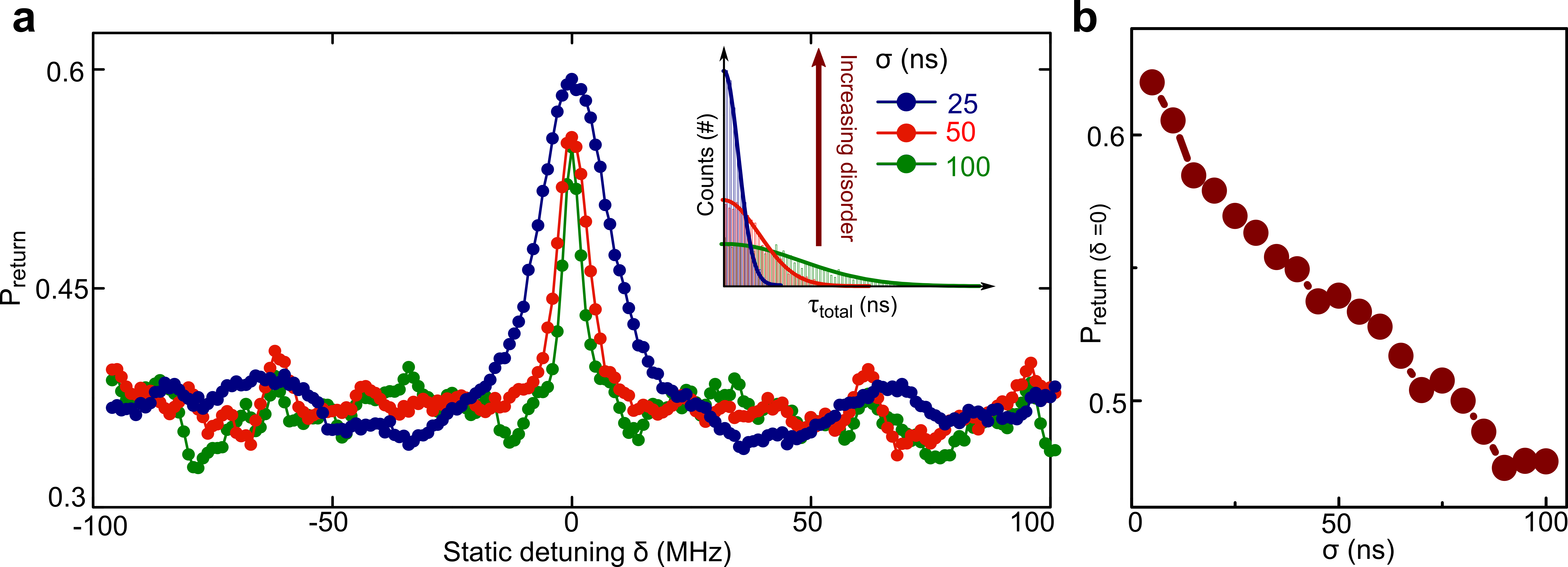
Figure 3: Simulating the disorder dependence of weak localization. a. Inset: Three distributions used for $\tau_{\text{total}}$ values, with standard deviations $\sigma=100$, 50 and 20 ns. Main panel: $P_{\text{return}}$ as a function of $\delta$ for the distributions shown in the inset. b. $P_{\text{return}}$ at zero detuning as a function of the distribution width, showing the return probability increasing as the distribution is reduced.

In Fig. 2(a), we show the experimental $P_{\text{return}}$ versus static detuning $\delta$ for six different $T_{\varphi^{\text{eff}}}$, corresponding to magneto-resistance measurements at six different temperatures. For all data sets, the probability $P_{\text{return}}$ has its maximum at $\delta=0$, where time-reversal symmetry is protected. As $\delta$ moves away from zero, $P_{\text{return}}$ rapidly decreases until it reaches an average value of approximately $0.35$, about which it fluctuates randomly. The reduction in $P_{\text{return}}$ with increasing $|\delta|$ is consistent with the well-known negative magneto-resistance in the mesoscopic system.

With the basic phenomena established, we focus on the small detuning region to investigate the role of quantum coherence, through variations in $T_{\varphi^{\text{eff}}}$ (Fig. 2(a) inset). While the overall structure remains unchanged, the $P_{\text{return}}$ peak grows as $T_{\varphi^{\text{eff}}}$ is increased; the peak rises from $\sim 0.46$ for $T_{\varphi^{\text{eff}}}=117$ ns to $\sim 0.53$ for $T_{\varphi^{\text{eff}}}=220$ ns, consistent with the temperature dependence of weak localization, where lower temperatures and thus longer phase coherent lengths increase the magnitude of the negative magneto-resistance peak Bishop1982 .

As they are performed on a highly controlled quantum system, our experimental results can be understood within the Tavis-Cummings model (see supplement). As shown in Fig. 2b, we numerically evaluated $P_{\text{return}}$ versus $\delta$, using the same six $T_{\varphi^{\text{eff}}}$ in the experiment. In the calculations we have also included the energy dissipation time for each qubit, $T_{1}\sim 500$ ns. Except for details in the aperiodic structures, the numerical results agree remarkably well with our experimental observations.

Just as the phase coherence length $L_{\varphi}$ can be extracted from magneto-resistance measurements displaying weak localization, we can extract the effective coherence time $T_{\varphi^{\text{eff}}}$ from our measured $P_{\text{return}}(\delta)$. We measured $P_{\text{return}}(\delta=0)$ for various $\tau_{\pi}/\tau_{\text{total}}$, and subsequently extracted $T_{\varphi^{\text{eff}}}$ from the height of the $P_{\text{return}}$ peak, based on the relationship $\Delta P_{\text{return}}\propto\frac{1}{2}\exp(-(\left\langle t\right\rangle/T_{\varphi^{\text{eff}}})^{2})\exp(-\left\langle t\right\rangle/T_{1})$ (see the theory section in supplement). The result is shown in Fig. 2c, compared with $T_{\varphi^{\text{eff}}}$ determined using conventional Ramsey-type measurements. As $\tau_{\pi}/\tau_{\text{total}}$ increases from 0 to 0.5, $T_{\varphi^{\text{eff}}}$ increases as expected due to the cancellation of the qubit frequency drifts. We find reasonable agreement between the values of $T_{\varphi^{\text{eff}}}$ as measured with the two techniques, with deviations possibly caused by the finite number of ensembles in the simulation.

The importance of the weak localization effect is not only because it reveals quantum coherence in transport, but also because it is a precursor to strong localization, also known as Anderson localization Anderson1958 . In the strong disorder limit, quantum interference completely halts carrier transmission, producing a disorder-driven metal-to-insulator transition. Our quantum circuit simulator allows us to directly and separately tune the level of disorder, by varying the distribution of pulse durations $\tau_{\mbox{total}}$, in contrast with the mesoscopic system where tuning the disorder level typically changes other parameters such as carrier density Lin1993 ; Ishiguro1992 ; Niimi2010 .

To measure the return probability $P_{\text{return}}$ as a function of disorder, we average 100 random detuning pulse sequences with $\tau_{\text{total}}$ , where $\tau_{\text{total}}$ is randomly generated from a Gaussian distribution with width $\sigma$. We used a Gaussian distribution to mimic the diffusive nature of electron transport. The electron displacement at a given time has a Gaussian distribution, where narrower distributions correspond to greater disorder. Correlating the disorder with $\sigma$, we simulate weak localization at increasing disorder levels by reducing $\sigma$ from 100 to 50 to 25 ns.

The experimentally measured $P_{\text{return}}$ versus $\delta$ for these three simulated disorder levels is shown in Fig. 3a. While the baseline value remains unchanged, the height of the zero-detuning peak grows as we reduce $\sigma$. This growth in the peak height with smaller $\sigma$ agrees with the observation that an increased degree of disorder enhances localization in electron transport Lin1993 ; Ishiguro1992 ; Niimi2010 .

In order to find the signature of a disorder-driven metal-insulator transition, we focus on $P_{\text{return}}$ at $\delta=0$ while continuously reducing $\sigma$. The results, using $\tau_{\pi}/\tau_{\text{total}}=0.5$ for maximum $T_{\varphi^{\text{eff}}}$, are displayed in Fig. 3b. Reducing $\sigma$ results in an increase of the photon return probability, with $P_{\text{return}}(\delta=0)$ increasing from 0.47 at $\sigma=200$ ns to 0.62 at $\sigma=10$ ns. However, there is no clear indication of an abrupt transition to a fully localized state, which would correspond to $P_{\text{return}}$ approaching unity. The metal-insulator transition is therefore not observed in our current experiment. Observing this transition likely requires further increasing the level of disorder, i.e., increasing the ratio $T_{\varphi^{\text{eff}}}/\sigma$. Such studies are now possible using the 100-fold improvement in coherence time recently achieved using the Xmon qubit Barends2013 , and are currently underway.

In closing, we comment on the aperiodic structure at the baseline of $P_{\text{return}}$ that appears in both the experimental and numerical results. The shape of this structure is independent of $T_{\varphi^{\text{eff}}}$, while the fluctuation amplitude increases with increasing $T_{\varphi^{\text{eff}}}$. These resemble the universal conductance fluctuations associated with weak localization in mesoscopic systems: Both emerge from the frequency beating of the interference fringes Umbach1984 ; Lee1985 ; Stone1985 . Our experiment, however, does not include the cross-interference terms between trajectories that do not have time-reversed symmetry, so it is unclear if the fluctuation amplitudes here have a universal value independent of the experimental details. Measurements on a quantum system of large size are required to clarify this issue.

I Method

The quantum circuit used in this experiment uses the same circuit design as that used to implement Shor’s algorithm Lucero2012 . As shown in Fig.1b, it is composed of four superconducting phase qubits, each connected to a memory resonator and all symmetrically coupled to a single central coupling resonator. The chip was fabricated using conventional multi-layered lithography and reactive ion etching. The different metal Al layers were deposited using DC sputtering and the low-loss dielectric $a$-Si was deposited throught plasma-enhanced chemical vapor deposition (PECVD).

The flux-biased phase qubit includes a $1$ pF parallel plate capacitor and a 700 pH double-coiled inductor shunted with a Al/AlOx/Al Josephson junction. The phase qubit can be modeled as a nonlinear LC oscillator, whose nonlinearity arises from the Josephson junction. Adjusting the flux applied to the qubit loop, we can modulate the phase across the junction and consequently tune the qubit frequency. We are thus able to tune the qubit frequency over more than several hundred MHz without introducing any significant variation in the qubit phase coherence. This property is crucial for this implementation of the simulation protocol.

II Acknowledgments

Devices were made at the UC Santa Barbara Nanofabrication Facility, part of the NSF-funded National Nanotechnology Infrastructure Network. This research was funded by the Office of the Director of National Intelligence (ODNI), Intelligence Advanced Research Projects Activity (IARPA), through Army Research Office grant W911NF-10-1-0334. All statements of fact, opinion or conclusions contained herein are those of the authors and should not be construed as representing the official views or policies of IARPA, the ODNI, or the U.S. Government.

III Author contribution

Y.C. conceived and carried out the experiments, and analyzed the data. J.M.M. and A.N.C supervised the project, and co-wrote the manuscript with Y.C. and P.R.. P.R., M.M, D.S. and C.N. provided assistance in the data taking, data analysis and writing the manuscript. E.L. fabricated the sample. All authors contributed to the fabrication process, qubit design, experimental set-up and manuscript preparation.

IV Competing financial interests

The authors declare no competing finacial interests.

References

- (1) Feynman, R. Simulating physics with computers. Int. J. Theor. Phys. 21, 467488 (1982).
- (2) I. Buluta and F. Nori, Quantum simulators, Science 326, 108-111 (2009).
- (3) A. Aspuru-Guzik and P. Walther, Photonic quantum simulators, Nature Phys. 8, 285-291 (2012).
- (4) R. Blatt and C. F. Roos, Quantum simulations with trapped ions, Nature Phys. 8, 277-284 (2012).
- (5) I. Bloch, J. Dalibard, and S. Nascimbene, Quantum simulations with ultracold quantum gases, Nature Phys. 8, 267-276 (2012).
- (6) M. Neeley, M. Ansmann, R. C. Bialczak, M. Hofheinz, E. Lucero, A. D. O’Connell, D. Sank, H.Wang, J.Wenner, A. N. Cleland, M. R. Geller, and J. M. Martinis, Emulation of a quantum spin with a superconducting phase qudit, Science, 325, 722-725 (2009).
- (7) J. Raftery, D. Sadri, S. Schmidt, H. E. Tï¿œreci, and A. A. Houck, Observation of a dissipationinduced classical to quantum transition, arXiv: 1312.2963 (2013).
- (8) A. A. Houck, H. E. Tureci, and J. Koch, On-chip quantum simulation with superconducting circuits, Nature Phys. 8, 292-299 (2012).
- (9) G. Bergmann, Weak localization in thin lms : a time-of-ight experiment with conduction electrons, Physics Reports 107, 1-58, 1984.
- (10) F. Pierre, A. B. Gougam, A. Anthore, H. Pothier, D. Esteve, and N. O. Birge, Dephasing of electrons in mesoscopic metal wires, Phys. Rev. B 68, 085413 (2003).
- (11) E. Lucero, R. Barends, Y. Chen, J. Kelly, M. Mariantoni, A. Megrant, P. O’Malley, D. Sank, 10 A. Vainsencher, J. Wenner, T. White, Y. Yin, A. N. Cleland, and J. M. Martinis, Computing prime factors with a josephson phase qubit quantum processor, Nature Phys. 8, 719-723 (2012).
- (12) M. Tavis and F. W. Cummings, Exact solution for an n-molecule-radiation-eld hamiltonian, Phys. Rev. 170, 379-384 (1968).
- (13) J. A. Mlynek, A. A. Abdumalikov, J. M. Fink, L. Steen, M. Baur, C. Lang, A. F. van Loo, and A. Wallra, Demonstrating w-type entanglement of dicke states in resonant cavity quantum electrodynamics, Phys. Rev. A 86, 053838 (2012).
- (14) E. L. Hahn, Spin echoes, Phys. Rev. 80, 580-594 (1950).
- (15) D. J. Bishop, R. C. Dynes, and D. C. Tsui, Magnetoresistance in si metal-oxide-semiconductor eld-eect transitors: Evidence of weak localization and correlation, Phys. Rev. B 26, 773-779 (1982).
- (16) P. W. Anderson, Absence of diusion in certain random lattices, Phys. Rev. 109, 1492-1505 (1958).
- (17) J. J. Lin and C. Y. Wu, Electron-electron interaction and weak-localization effects in ti-al alloys, Phys. Rev. B 48, 5021-5024 (1993).
- (18) T. Ishiguro, H. Kaneko, Y. Nogami, H. Ishimoto, H. Nishiyama, J. Tsukamoto, A. Takahashi, M. Yamaura, T. Hagiwara, and K. Sato, Logarithmic temperature dependence of resistivity in heavily doped conducting polymers at low temperature, Phys. Rev. Lett. 69, 660-663 (1992).
- (19) Y. Niimi, Y. Baines, T. Capron, D. Mailly, F.-Y. Lo, A. D. Wieck, T. Meunier, L. Saminadayar, and C. Bauerle, Quantum coherence at low temperatures in mesoscopic systems: Effect of disorder, Phys. Rev. B 81, 245306 (2010).
- (20) R. Barends, J. Kelly, A. Megrant, D. Sank, E. Jerey, Y. Chen, Y. Yin, B. Chiaro, J. Mutus, C. Neill, P. O’Malley, P. Roushan, J. Wenner, T. C. White, A. N. Cleland, and J. M. Martinis, Coherent josephson qubit suitable for scalable quantum integrated circuits, Phys. Rev. Lett. 111, 080502 (2013).
- (21) C. P. Umbach, S. Washburn, R. B. Laibowitz, and R. A. Webb, Magnetoresistance of small, quasi-one-dimensional, normal-metal rings and lines, Phys. Rev. B 30, 4048-4051 (1984).
- (22) P. A. Lee and A. D. Stone, Universal conductance uctuations in metals, Phys. Rev. Lett. 55, 1622-1625 (1985).
- (23) A. D. Stone, Magnetoresistance uctuations in mesoscopic wires and rings, Phys. Rev. Lett. 54, 2692-2695 (1985).