Shear thickening, frictionless and frictional rheologies in non-Brownian suspensions

Abstract

Particles suspended in a Newtonian fluid raise the viscosity and also generally give rise to a shear-rate dependent rheology. In particular, pronounced shear thickening may be observed at large solid volume fractions. In a recent article (R. Seto, R. Mari, J. F. Morris, and M. M. Denn., Phys. Rev. Lett., 111:218301, 2013) we have considered the minimum set of components to reproduce the experimentally observed shear thickening behavior, including Discontinuous Shear Thickening (DST). We have found frictional contact forces to be essential, and were able to reproduce the experimental behavior by a simulation including this physical ingredient along with viscous lubrication. In the present article, we thoroughly investigate the effect of friction and express it in the framework of the jamming transition. The viscosity divergence at the jamming transition has been a well known phenomenon in suspension rheology, as reflected in many empirical laws for the viscosity. Friction can affect this divergence, and in particular the jamming packing fraction is reduced if particles are frictional. Within the physical description proposed here, shear thickening is a direct consequence of this effect: as the shear rate increases, friction is increasingly incorporated as more contacts form, leading to a transition from a mostly frictionless to a mostly frictional rheology. This result is significant because it shifts the emphasis from lubrication hydrodynamics and detailed microscopic interactions to geometry and steric constraints close to the jamming transition.

I Introduction

I.1 Shear thickening

Suspensions (solid particles immersed in a fluid) exhibit a wide range of rheological behaviors, including shear thinning, shear thickening, and finite normal stress differences. Shear thickening [Barnes, 1989; Mewis and Wagner, 2011; Brown and Jaeger, 2014], where the viscosity increases with shear rate even if the suspending fluid is Newtonian, is a particularly intriguing phenomenon. In the extreme case of Discontinuous Shear Thickening (DST; for early descriptions see the work of Williamson [1930]; Williamson and Hecker [1931]; Freundlich and Roder [1938]), which is observed at high volume fractions of solid material, the viscosity can increase by several orders of magnitude at a critical shear rate. Note that we do not include here the irreversible shear thickening occurring due to particle aggregation (as seen for example in fumed silica [Crawford et al., 2013]) under the name DST.

The variety of systems showing a DST suggests that this may be a universal behavior that is obtained with a minimum set of physical ingredients. Even though most of the data available are for Brownian suspensions (that is, sub-micrometer particles) [Metzner and Whitlock, 1958; Hoffman, 1972; Bender and Wagner, 1995, 1996; Frith et al., 1996; Fagan and Zukoski, 1997; Boersma, Laven, and Stein, 1990; D’Haene, Mewis, and Fuller, 1993; O’Brien and Mackay, 2000; Maranzano and Wagner, 2001b, a, 2002], thermal motion does not seem necessary to observe DST, as experiments with micrometer scale [Boersma, Laven, and Stein, 1990; Lootens et al., 2004, 2005; Larsen et al., 2010] or larger particles [Freundlich and Roder, 1938; Bertrand, Bibette, and Schmitt, 2002; Brown and Jaeger, 2009, 2012; Fall et al., 2010, 2012] show. Inertia has also been associated with the existence of shear thickening in suspensions [Lemaître, Roux, and Chevoir, 2009; Fall et al., 2010; Trulsson, Andreotti, and Claudin, 2012; Fernandez et al., 2013; Kawasaki, Ikeda, and Berthier, 2014], based on the initial ideas of Bagnold [1954], but the Bagnoldian scaling of a viscosity proportional to the shear rate is clearly milder than the abrupt shear thickening observed in experiments. More importantly the thickening due to inertia arises at Stokes number $\mbox{{St}}\equiv\rho a^{2}\dot{\gamma}/\eta_{0}$ (with $\dot{\gamma}$ the shear rate, $\eta_{0}$ the viscosity of the fluid phase, and $\rho$ and $a$ the mass density and size of the solid particles, respectively) of order $\mbox{{St}}\approx 1$ in the simulations [Trulsson, Andreotti, and Claudin, 2012; Fernandez et al., 2013; Kawasaki, Ikeda, and Berthier, 2014], which contrasts with the values of at most $\mbox{{St}}\approx 10^{-3}$ found in experiments (see for example [Maranzano and Wagner, 2001b; Fall et al., 2010; Brown and Jaeger, 2012]). Thus inertia is not necessary for DST in the conditions probed by rheometric flows. (Flows involving significantly larger particles, say in the $\mathrm{mm}$ range, or significantly larger shear rates $\dot{\gamma}\gg$1\text{\,}{\mathrm{s}}^{-1}$$, can probe the regime where inertia matters).

Indeed, the apparently simple experimental system of nearly rigid non-Brownian neutrally buoyant particles immersed in a Newtonian fluid exhibits DST in the Stokes regime [Brown and Jaeger, 2009, 2012], indicating that the phenomenon stems from a rather restricted set of simple ingredients. The puzzle has very few pieces. In the Stokes regime, however, non-Brownian neutrally buoyant hard spheres in a Newtonian fluid will create a suspension whose rheology is independent of shear rate, as there is only one force scale, the hydrodynamic one (we will further explain this fact in Sec. II.2.1). So there cannot be too few pieces.

I.2 Fluid mechanics and granular physics perspectives

The flow of suspensions has historically been studied from a fluid mechanics perspective, and the emphasis has been on a description based on hydrodynamic interactions. Suspensions are usually described as hard particles immersed in a Newtonian fluid, interacting through hydrodynamics (including Brownian forces) and sometimes an additional soft repulsive potential (approximating an electric double-layer or mimicking polymer coating, for instance). They are typically studied in the Stokes flow regime, at vanishing particle Reynolds number $\mbox{{Re}}\equiv\rho_{0}a^{2}\dot{\gamma}/\eta_{0}$ (with $\rho_{0}$ the mass density of the fluid phase) and Stokes number. The key point is that the hard cores of the particles are treated as boundary conditions for the Stokes equations that describe the fluid phase; the particles never directly generate forces through contacts. This treatment is self-consistently justified by the fact that the Stokes flow between two rigid surfaces leads to a lubrication force whose resistance coefficient diverges at contact, effectively preventing two particles from colliding. Within this framework, shear thickening is explained by the creation at large shear rates of locally denser clusters of particles (hydro-clusters), which are highly dissipative due to the singular lubrication flows between the particles [Brady and Bossis, 1985; Bender and Wagner, 1996; Melrose and Ball, 2004a; Wagner and Brady, 2009]. While this purely fluid mechanical point of view is able to describe the flow and rheology of moderately concentrated suspensions, it seems unable to explain the abrupt shear thickening observed in highly concentrated suspensions. Simulations by Stokesian Dynamics give a weak logarithmic shear thickening [Brady and Bossis, 1988; Bossis and Brady, 1989; Phung, Brady, and Bossis, 1996; Foss and Brady, 2000; Melrose and Ball, 2004b], thereby raising the issue of the validity of this approach at high volume fractions. Moreover, DST is also observed in athermal suspensions, where the shear rate dependence introduced by the Brownian force scale disappears: in this regime, a purely hydrodynamic perspective would predict a shear-rate independent rheology.

In the past few years, new ideas have emerged from the granular rheology perspective. Boyer, Guazzelli, and Pouliquen [2011] developed an analogy between the rheology of suspensions and the rheology of granular materials. In dry granular flow, the rheology depends on the ratio between inertia and particle pressure [Deboeuf et al., 2009]: if the inertia dominates, particles bounce around and the stresses are essentially due to momentum exchange based on collisions (a “granular gas” regime), whereas if the pressure dominates, particles are forced to stay at contact and the stresses are dominated by contact force chains (a “granular packing” regime). This perspective can be incorporated in a dimensionless inertial number $I\equiv\dot{\gamma}d\sqrt{\rho/\Pi}$ [da Cruz et al., 2005], where $d$ is the diameter of the solid particles, $\rho$ their density, and $\Pi$ the particle pressure. Similarly, for suspensions in the Stokes regime there is a viscous number $I_{\mathrm{v}}\equiv\eta_{0}\dot{\gamma}/\Pi$, where $\eta_{0}$ is the viscosity of the suspending fluid, which compares viscous dissipation to the particle pressure [Boyer, Guazzelli, and Pouliquen, 2011]. The stresses can be dominated either by viscous dissipation if $I_{\mathrm{v}}\gg 1$ (when particles are far apart) or by a contact network if $I_{\mathrm{v}}\ll 1$. This results in constitutive laws for the viscosity and other stress components and for the volume fraction that are unique functions of $I_{\mathrm{v}}$. One can anticipate that the regimes $I\ll 1$ and $I_{\mathrm{v}}\ll 1$, both of which are dominated by the approach to the jamming transition, will share some similarities. Indeed, they do share a power-law scaling (typical of the jamming transition) between particle pressure and distance to the jamming point $\Pi\sim(\phi_{\mathrm{J}}-\phi)^{-\lambda}$ [Forterre and Pouliquen, 2008; Boyer, Guazzelli, and Pouliquen, 2011]. The scaling is the same for the other stress components, including the important case of shear stress $\sigma\sim(\phi_{\mathrm{J}}-\phi)^{-\lambda}$. These power laws are now argued to be a generic behavior close to jamming [Lerner, Düring, and Wyart, 2012; Andreotti, Barrat, and Heussinger, 2012], though the value of the exponent $\lambda$ might be system dependent (it might depend on shape or friction for instance). With these ideas, the emphasis has shifted from hydrodynamics and detailed microscopic interactions to geometry and steric constraints close to the jamming transition.

While those new ideas have proven to be successful in explaining some of the rheology at high volume fractions [Boyer, Guazzelli, and Pouliquen, 2011; Trulsson, Andreotti, and Claudin, 2012; Lerner, Düring, and Wyart, 2012], they cannot account for non-Newtonian behavior in the Stokes regime. The case of DST is particularly puzzling: whereas intuition suggests that DST is a manifestation of jamming [Cates et al., 1998; Bertrand, Bibette, and Schmitt, 2002; Lootens, Van Damme, and Hébraud, 2003; Hébraud and Lootens, 2005; Brown and Jaeger, 2009], DST is not captured by the $I_{\mathrm{v}}$-based rheology, which predicts no shear rate dependence in the Stokes regime [Lerner, Düring, and Wyart, 2012; Trulsson, Andreotti, and Claudin, 2012], and reduces to a $\phi$-dependent rheology [Boyer, Guazzelli, and Pouliquen, 2011]. Simply stated, this rheology predicts the correct volume fraction dependence of the viscosity at fixed shear rate, but completely fails at predicting the shear rate dependence at fixed volume fraction. Again, it is worth noticing that this absence of shear rate dependence hints at a missing force (or time) scale in the description of dense suspensions.

I.3 This work

In this article, which extends and complements a previous publication [Seto et al., 2013], we show how jamming is related to shear thickening and how to escape the apparent contradiction described above. The starting point is to note that the jamming transition, while it exhibits some generic features that are independent of the microscopic interactions like the scalings described above, retains a clear signature of the microscopic details in the volume fraction at which it occurs. For instance, it is well known that jamming can occur anywhere between $\phi_{\mathrm{J}}^{\mu=\infty}\approx 0.55$ and $\phi_{\mathrm{J}}^{\mu=0}\approx 0.64$ depending on the friction coefficient $\mu$ between the grains [Silbert et al., 2002; Jerkins et al., 2008; Song, Wang, and Makse, 2008; Silbert, 2010]. This means that the relation $\phi(I_{\mathrm{v}})$ actually depends on $\mu$, which in turn implies that the viscosity $\eta(\phi)$ depends on $\mu$. Therefore, if there exists a mechanism such that $\mu$ (or an effective friction coefficient) varies with the shear rate $\dot{\gamma}$, one can obtain a non-Newtonian rheology within the framework of Boyer, Guazzelli, and Pouliquen [2011]. This mechanism has to be associated with an extra force scale besides the hydrodynamic one in order to provide the shear-rate dependence.

We introduced such a mechanism in the recent article [Seto et al., 2013], and here we thoroughly explore its consequences through numerical simulations of dense (i.e., highly concentrated) non-Brownian suspensions under simple shear flow. We note that two other recent papers have independently introduced similar but somewhat different mechanisms to achieve a rate-dependent friction coefficient $\mu(\dot{\gamma})$ in simple shear flow simulations [Fernandez et al., 2013; Heussinger, 2013]. Both of them prove that interparticle friction is essential to shear thickening of dense suspensions. In contrast to those works, the present work however show that inertia is inessential to this phenomenon, as we obtain it in an overdamped simulation (see next Section). This is important because results coming from simulations including inertia gives shear thickening at shear rates that are several orders of magnitude larger than the experimental values (see previous Sec. I.1). We show here that our inertialess model gives a quantitative description of shear thickening (see Conclusion Sec. V).

The present work shows the importance of frictional contacts in dense suspension rheology. Of course, particles must form contacts during flow in order for the rheology to depend on the friction coefficient, and here we come up against one consequence of the fluid mechanics perspective. In fact, it is known that particles do come in contact under flow, even in the dilute limit, perhaps due to surface roughness [Davis, 1992; Zhao and Davis, 2002; Lootens et al., 2005; Blanc, Peters, and Lemaire, 2011]. One simply has to accept that those contacts, though not essential to the rheology of dilute or semi-dilute suspensions (as the successes of Stokesian Dynamics demonstrate), become important at large volume fractions. But contacts are a necessity if one thinks of the large volume-fraction limit of jamming ($I_{\mathrm{v}}\to 0$): there is no more room in this limit for lubrication films between particles, and contacts must proliferate and dominate the rheology. Besides enforcing the geometric constraint of no overlapping particles, those contacts bring a new restriction to reorganization at the microscopic level: they carry significant tangential forces due to friction. It is worth noting that even though the close-range hydrodynamics (i.e., lubrication forces) also generate some tangential forces, they are of a fundamentally different nature. For a relative motion between two nearby particles, the normal lubrication force diverges as the inverse of the interparticle gap, whereas the tangential lubrication force diverges only logarithmically with vanishing gap, which means that the effective friction coefficient vanishes in the limit of a small gap. Thus lubrication, as in its literal meaning, provides very little resistance to relative tangential motion compared to relative normal motion. This stands in contrast to the frictional contact forces, for which the friction coefficient is finite; i.e., tangential and normal contact forces are of comparable scale. It follows that the constraint introduced by contact friction is much more efficient at increasing the viscosity than is lubrication.

Describing the physics of contact and motion when the gap between two particles in a suspension is smaller than, say, $1\text{\,}\mathrm{nm}$, is not an easy task. Moreover, one cannot expect to find generic behavior, as interactions will vary depending on the nature of the solid particles and of the suspending fluid. However, this level of detail may not be essential to understanding the physics that emerges at a macroscopic level. At high volume fractions it is reasonable to expect that the singularity associated with the jamming transition will dominate the rheology of suspensions. Our approach in this work is thus to study the rheology of minimal model systems that include hydrodynamics, a repulsive interaction, and frictional contacts between particles. These interactions, while being realistic, will be simplified to their essence.

II Models and methods

In this section, we will describe our numerical model of a dense non-Brownian suspension under shear flow [Denn and Morris, 2014]. We intend to have a minimal model containing as few physical elements as possible while exhibiting a DST. Even if the model is intended to be as generic as possible, a few parameter choices are necessary. For those choices, we try to set values that correspond to a realistic interpretation of a suspension of hard (say, silica) spheres with radius in the $1\text{\,}\mathrm{\SIUnitSymbolMicro m}10\text{\,}\mathrm{\SIUnitSymbolMicro m}$ range, density matched (or such that the sedimentation occurs over times much larger than the inverse shear rate) and charge stabilized. The only parameter that takes an unrealistic value is the particles’ stiffness, which is smaller in the simulations than in a typical experimental system. A stiffness comparable to experimental values for silica (or even PMMA), would require the use of very small time steps in the simulation in order to resolve the dynamics of the contacts which correspond to an overlap in the $\mathrm{nm}$ range. We however circumvent this problem by tuning the particle stiffness with applied shear rate such that we get rid of particle deformation effects in the rheology (see Sec. II.1.3 and Appendix B for details).

II.1 Merging hydrodynamic interactions and granular contact models

II.1.1 Equations of motion

In a suspension, the flow of the fluid is described by the Navier-Stokes equation, while the motion of the particles is given by Newton’s equation of motion:

$$\bm{m}\cdot\frac{\mathrm{d}}{\mathrm{d}t}\begin{pmatrix}\bm{U}\\ \bm{\Omega}\end{pmatrix}=\sum_{\alpha}\begin{pmatrix}\bm{F}_{\alpha}(\bm{U},\bm{\Omega},\bm{r})\\ \bm{T}_{\alpha}(\bm{U},\bm{\Omega},\bm{r})\end{pmatrix},$$ (1)

where $\bm{m}$ is the mass/moment-of-inertia matrix, $\bm{U}$ and $\bm{\Omega}$ are the translational and rotational velocity vectors, and $\bm{F}_{\alpha}$ and $\bm{T}_{\alpha}$ are the force and torque vectors, respectively. The right-hand side consists of two different types of forces: some depend only on the configurations $\bm{r}$ of the particles (e.g., forces derived from a potential), but some also depend on the velocities $\bm{U}$ and $\bm{\Omega}$, including inelastic contact forces (e.g., contacts with dashpot terms) and fluid-particle interactions (hydrodynamic interactions).

We will study the rheology of this suspension under an imposed simple shear flow field $\bm{U}^{\infty}(\bm{r})$ expressed using the vorticity $\bm{\Omega}^{\infty}$ and the rate-of-strain tensor $\bm{E}^{\infty}$ as

$$\bm{U}^{\infty}(\bm{r})=\bm{\Omega}^{\infty}\times\bm{r}+\bm{E}^{\infty}\cdot\bm{r}.$$ (2)

At a shear rate $\dot{\gamma}$, a simple shear flow corresponds to the following nonzero elements: $\Omega^{\infty}_{3}=\dot{\gamma}/2$ and $E^{\infty}_{12}=E^{\infty}_{21}=\dot{\gamma}/2$.

In many experimental flows, including the ones for which shear thickening is typically observed, the particle Reynolds number and the Stokes number are very small due to the small size of the suspended particles. This means that the equation of motion for the particles can be studied in its overdamped limit, which is simply a quasi-static force balance equation. As will be discussed in Secs. II.1.2, II.1.3, and II.2 below, in this regime the velocity dependence coming from the hydrodynamic interactions and the contact forces has a linear form, and the force balance equation can be written as a linear algebraic relation having the form

$$\bm{0}=\bm{R}\cdot\begin{pmatrix}\bm{U}-\bm{U}^{\infty}\\ \bm{\Omega}-\bm{\Omega}^{\infty}\end{pmatrix}+\begin{pmatrix}\bm{F}(\bm{r})\\ \bm{T}(\bm{r})\end{pmatrix},$$ (3)

Therefore, our simulation of a suspension under a simple shear flow in the Stokes regime requires solving (3) for the velocities, and obtaining the positions $\bm{r}$ of the particles at any time $t$ through time integration of these velocities.

II.1.2 Hydrodynamic interactions

In principle, hydrodynamic interactions can be determined by solving the Stokes equations, but this is extremely expensive from a computational view point. For dense suspensions, however, the dominant hydrodynamic interactions come from the fluid flow in the narrow gaps between nearby solid particles [Ball and Melrose, 1997], because the resistance to relative motion becomes singular when the gaps are vanishingly small. They give rise to pair-wise short range lubrication forces (as opposed to the many-body nature of the full, long-range hydrodynamic interactions). As a consequence, the linear relations between velocities and hydrodynamic forces simply contain a contribution from the Stokes drag and a contribution from the lubrication:

$$\begin{pmatrix}\bm{F}_{\mathrm{H}}\\ \bm{T}_{\mathrm{H}}\end{pmatrix}=-\bigl{(}\bm{R}_{\mathrm{Stokes}}+\bm{R}_{\mathrm{Lub}}\bigr{)}\cdot\begin{pmatrix}\bm{U}-\bm{U}^{\infty}\\ \bm{\Omega}-\bm{\Omega}^{\infty}\\ \end{pmatrix}+\bm{R}^{\prime}_{\mathrm{Lub}}:\bm{E}^{\infty}.$$ (4)

$\bm{R}_{\mathrm{Stokes}}$ is a diagonal matrix giving Stokes drag forces and torques, and $\bm{R}_{\mathrm{Lub}}$ and $\bm{R}^{\prime}_{\mathrm{Lub}}$ are sparse matrices [Ball and Melrose, 1997].

Consistent with our choice of keeping only physically relevant near-distance interactions, we use only the leading terms for the resistance matrices. Physically, the terms included in our model correspond to the squeeze, shear, and pump modes of Ball and Melrose [1997] (we do not consider their twist mode, as it is not associated with a divergence of the resistance at contact, and is thus subdominant). Defining the non-dimensional gap $h^{(i,j)}$ between particles $i$ and $j$ having radii $a_{i}$ and $a_{j}$ as $h^{(i,j)}\equiv 2(r^{(i,j)}-a_{i}-a_{j})/(a_{i}+a_{j})$ and the center-to-center unit vector $\bm{n}_{ij}\equiv(\bm{r}^{(j)}-\bm{r}^{(i)})/r^{(i,j)}$ with $r^{(i,j)}\equiv|\bm{r}^{(j)}-\bm{r}^{(i)}|$, the modes associated with relative displacements respectively along and tangential to $\bm{n}_{ij}$ have singular behaviors with leading terms diverging as $1/h^{(i,j)}$ and $\log(1/h^{(i,j)})$ [Jeffrey and Onishi, 1984; Jeffrey, 1992]. The consequence of the singularity in the squeeze mode (i.e., along $\bm{n}_{ij}$) is that there should not be any contact between particles [Ball and Melrose, 1995]. However, as mentioned in the introduction, this statement is only true for perfectly idealized situations, and not realistic even for model experimental systems consisting of spherical particles due to, for example, a finite surface roughness [Davis, 1992; Zhao and Davis, 2002; Lootens et al., 2005; Blanc, Peters, and Lemaire, 2011] or a breakdown of the continuity assumption for the fluid at the molecular mean free path scale [Ho and Tai, 1998]. In order to mimic this reality, we regularize the singularities arising in the lubrication resistances by inserting a small cutoff length scale $\delta$ [Trulsson, Andreotti, and Claudin, 2012], which can be thought of as the length scale of the particle surface roughness; the leading terms we use for normal and tangential displacements then behave as $1/(h^{(i,j)}+\delta)$ and $\log(1/(h^{(i,j)}+\delta))$. In the simulations, we set $\delta=10^{-3}$, giving large enough resistance for the squeeze mode compared to the typical hydrodynamic force. This value is typical for non-Brownian particles [Davis, 1992; Blanc, Peters, and Lemaire, 2011]. The detailed expressions for the resistance matrices $\bm{R}_{\mathrm{Lub}}$ and $\bm{R}^{\prime}_{\mathrm{Lub}}$ are given in Appendix A.

II.1.3 Contact model

There are several models that one can use to describe frictional contacts between particles. We use a stick/slide friction model employing springs and dashpots that is commonly used in granular physics [Cundall and Strack, 1979; Luding, 2008]. The normal and tangential components of the force and the torque for particles having radii $a_{i}$ and $a_{j}$ are obtained as

$$\begin{split}\bm{F}_{\mathrm{C,nor}}^{(i,j)}&=k_{\mathrm{n}}h^{(i,j)}\bm{n}_{ij}+\gamma_{\mathrm{n}}\bm{U}_{\mathrm{n}}^{(i,j)},\\ \bm{F}_{\mathrm{C,tan}}^{(i,j)}&=k_{\mathrm{t}}\bm{\xi}^{(i,j)},\\ \bm{T}_{\mathrm{C}}^{(i,j)}&=a_{i}\bm{n}_{ij}\times\bm{F}_{\mathrm{C,tan}}^{(i,j)},\end{split}$$ (5)

and fulfill Coulomb’s friction law $\bigl{|}\bm{F}_{\mathrm{C,tan}}^{(i,j)}\bigr{|}\leq\mu\bigl{|}\bm{F}_{\mathrm{C,nor}}^{(i,j)}\bigr{|}$. In the above expressions, $k_{\mathrm{n}}$ and $k_{\mathrm{t}}$ are the normal and tangential spring constants, respectively, and $\gamma_{\mathrm{n}}$ is the damping constant. The normal and tangential velocities are $\bm{U}_{\mathrm{n}}^{(i,j)}\equiv\bm{n}_{ij}\bm{n}_{ij}\cdot(\bm{U}^{(j)}-\bm{U}^{(i)})$ and $\bm{U}_{\mathrm{t}}^{(i,j)}\equiv(\bm{I}-\bm{n}_{ij}\bm{n}_{ij})\cdot[\bm{U}^{(j)}-\bm{U}^{(i)}-(a_{i}\bm{\Omega}^{(i)}+a_{j}\bm{\Omega}^{(j)})\times\bm{n}_{ij}]$. Finally, the quantity $\bm{\xi}^{(i,j)}$ is the tangential spring stretch. This contact model could be made more general, but at the price of numerical difficulties; see Appendix B.

The computation of the tangential spring stretch $\bm{\xi}^{(i,j)}$, described in the following, requires some care, as we have to impose Coulomb’s law. We apply an algorithm described in Luding [2008]. At the time $t_{0}$ at which the contact ${(i,j)}$ is created, we set an unstretched tangential spring $\bm{\xi}^{(i,j)}(t_{0})=\bm{0}$. At any further time step $t$ in the simulation, the tangential stretch $\bm{\xi}^{(i,j)}(t)$ is incremented according to the value of a “test” force $\bm{F}_{\mathrm{C,tan}}^{\prime(i,j)}(t+\mathrm{d}t)=k_{\mathrm{t}}\bm{\xi}^{\prime(i,j)}(t+\mathrm{d}t)$ with $\bm{\xi}^{\prime(i,j)}(t+\mathrm{d}t)=\bm{\xi}^{(i,j)}(t)+\bm{U}_{\mathrm{t}}^{(i,j)}(t)\mathrm{d}t$. If $\bigl{|}\bm{F}_{\mathrm{C,tan}}^{\prime(i,j)}(t+\mathrm{d}t)\bigr{|}\leq\mu\bigl{|}\bm{F}_{\mathrm{C,nor}}^{(i,j)}(t+\mathrm{d}t)\bigr{|}$, the contact is in a static friction state and we update the spring stretch and force as

$$\begin{split}&\bm{\xi}^{(i,j)}(t+\mathrm{d}t)=\bm{\xi}^{\prime(i,j)}(t+\mathrm{d}t),\\ &\bm{F}_{\mathrm{C,tan}}^{(i,j)}(t+\mathrm{d}t)=\bm{F}_{\mathrm{C,tan}}^{\prime(i,j)}(t+\mathrm{d}t).\end{split}$$ (6)

However, if $\bigl{|}\bm{F}_{\mathrm{C,tan}}^{\prime(i,j)}(t+\mathrm{d}t)\bigr{|}>\mu\bigl{|}\bm{F}_{\mathrm{C,nor}}^{(i,j)}(t+\mathrm{d}t)\bigr{|}$, the contact is in a sliding state and the spring and force are updated as

$$\begin{split}&\bm{\xi}^{(i,j)}(t+\mathrm{d}t)=\frac{\mu}{k_{\mathrm{t}}}\bigl{|}\bm{F}_{\mathrm{C,nor}}^{(i,j)}(t+\mathrm{d}t)\bigr{|}\bm{t}_{ij},\\ &\bm{F}_{\mathrm{C,tan}}^{(i,j)}(t+\mathrm{d}t)=k_{\mathrm{t}}\bm{\xi}^{(i,j)}(t+\mathrm{d}t),\end{split}$$ (7)

where the direction $\bm{t}_{ij}$ is the same as the one for the test force, i.e., $\bm{t}_{ij}\equiv\bm{F}_{\mathrm{C,tan}}^{\prime(i,j)}(t+\mathrm{d}t)/\bigl{|}\bm{F}_{\mathrm{C,tan}}^{\prime(i,j)}(t+\mathrm{d}t)\bigr{|}$. In this case, Coulomb’s law is not violated, as $\bigl{|}\bm{F}_{\mathrm{C,tan}}^{(i,j)}(t+\mathrm{d}t)\bigr{|}=\mu\bigl{|}\bm{F}_{\mathrm{C,nor}}^{(i,j)}(t+\mathrm{d}t)\bigr{|}$.

II.2 Other interactions, full models

II.2.1 Shear rate dependence: why Stokes hydrodynamics plus hard spheres is not enough

The shear-rate dependence of a suspension requires the existence of a time scale distinct from the inverse shear rate. A well known case is the one of Brownian suspensions, where the inverse shear rate competes with the Brownian diffusion time to give a shear-rate dependent rheology. This competition is adequately measured by a non-dimensionalized shear rate, the Péclet number, which is the ratio of the two time scales: $\mbox{{Pe}}\equiv 6\pi\eta_{0}a^{3}\dot{\gamma}/k_{\mathrm{B}}T$. This quantity can also be thought of as a ratio of two force scales: the typical hydrodynamic force and the typical Brownian force. Thus, a shear-rate dependent rheology generically requires at least one other force scale besides the hydrodynamic one.

Such a time scale does not exist for non-Brownian suspensions of hard spheres in the Stokes regime. The reason is straightforward: the hard sphere force has no typical value, and a hard-sphere contact between two particles can withstand any applied load. Therefore there is nothing with which to compare the hydrodynamic force. This means that the solutions of the force/torque balance equations (3) (i.e., the particle trajectories) are independent of the shear rate, leading to a shear-rate independent rheology. Notice that this conclusion holds whether the hard spheres are frictionless or frictional: Coulomb’s law does not introduce a force scale. There must be another force scale in the system to provide the shear-rate dependence.

An important point in our model is that, even if we try to mimic a hard sphere suspension, our contact forces actually are elastic forces, thus bringing a natural force scale $k_{\mathrm{n}}a$. We preserve the shear-rate independent hard sphere behavior by selecting the particle stiffness $k_{\mathrm{n}}$ such that the non-dimensional number based on the stiffness $6\pi\eta_{0}a\dot{\gamma}/k_{\mathrm{n}}$ remains much smaller than unity; i.e., we stay in the asymptotic regime of nearly hard particles. We describe the techniques we use to achieve this in our simulation in Appendix B.

II.2.2 A minimal model: critical-load friction

The first model we consider is an intentionally simplistic one, arguably the simplest model with an additional force scale besides the hydrodynamic force. Simplicity is the main motivation for this model, as it enables the clear physical discussion one can expect from a minimal model.

In this model (which we call Critical Load Model, CLM), we introduce an extra force scale in the friction law itself, namely a threshold normal load $F_{\mathrm{CL}}$ to activate friction. When the normal load is smaller than this threshold, particles interact as frictionless hard spheres. When the load is beyond the threshold, friction is activated. Overall, the friction law reads:

$$\bigl{|}\bm{F}_{\mathrm{C,tan}}^{(i,j)}\bigr{|}\leq\begin{cases}\mu\Bigl{(}\bigl{|}\bm{F}_{\mathrm{C,nor}}^{(i,j)}\bigr{|}-F_{\mathrm{CL}}\Bigr{)}&\text{for $\bigl{|}\bm{F}_{\mathrm{C,nor}}^{(i,j)}\bigr{|}\geq F_{\mathrm{CL}}$},\\ 0&\text{otherwise}.\end{cases}$$ (8)

We may consider the CLM as the short Debye length limit of the electrostatic repulsion model presented below (Sec. II.2.3).

II.2.3 Electrostatic repulsion model

An electrostatic repulsion is a simple and plausible interaction. Many experimental systems have such a force, as it stabilizes the suspension. Thus, we will consider an Electrostatic Repulsion Model (ERM) including this ingredient in the simplest form of a repulsive double-layer electrostatic force $\bm{F}_{\mathrm{R}}^{(i,j)}$ [Israelachvili, 2011]. If the Debye length $\kappa^{-1}$ is small compared to the radius of the particles, the approximate form

$$\bm{F}_{\mathrm{R}}^{(i,j)}(h)\simeq\begin{cases}-2F_{\mathrm{ER}}a_{i}a_{j}/(a_{i}+a_{j})e^{-\kappa(r^{(i,j)}-a_{i}-a_{j})}\bm{n}_{ij}&\text{if $h^{(i,j)}\geq 0$,}\\ -2F_{\mathrm{ER}}a_{i}a_{j}/(a_{i}+a_{j})\bm{n}_{ij}&\text{if $h^{(i,j)}<0$,}\end{cases}$$ (9)

can be used. In the simulations, we set $\kappa^{-1}=0.05a$, meaning a Debye length in the $0.1\text{\,}\mathrm{\SIUnitSymbolMicro m}$ range for particles of a few $\mathrm{\SIUnitSymbolMicro m}$; see Mewis and Wagner [2011].

II.3 Stress tensor and bulk rheology

The mechanical stress applied to the suspension arises from the several interactions included in the model: particles disturb the flow, creating hydrodynamic stresses, and they develop force chains via contacts (and/or electrostatic repulsion for the ERM).

The hydrodynamic stresslets acting on the particles are given by [Batchelor, 1970; Brady and Bossis, 1988]

$$\bm{S}_{\mathrm{H}}=-\bigl{(}\bm{R}_{\mathrm{Stokes}}^{S}+\bm{R}_{\mathrm{Lub}}^{S}\bigr{)}\cdot\begin{pmatrix}\bm{U}-\bm{U}^{\infty}\\ \bm{\Omega}-\bm{\Omega}^{\infty}\end{pmatrix}+\bm{R}_{\mathrm{Lub}}^{\prime S}:\bm{E}^{\infty},$$ (10)

where $\bm{S}_{\mathrm{H}}\equiv\bigl{(}\bm{S}_{\mathrm{H}}^{(1)},\dotsc,\bm{S}_{\mathrm{H}}^{(n)}\bigr{)}$ and the matrices $\bm{R}_{\mathrm{Lub}}^{S}$ and $\bm{R}_{\mathrm{Lub}}^{\prime S}$ contain leading terms of the lubrication resistances [Jeffrey and Onishi, 1984; Jeffrey, 1992] (see Appendix A) in a manner consistent with the hydrodynamic forces considered in Sec. II.1.2.

The stress due to the contact or repulsive force between particles $i$ and $j$ is simply written as

$$\bm{S}_{\mathrm{C}}^{(i,j)}=(\bm{r}^{(j)}-\bm{r}^{(i)})\bm{F}^{(i,j)}_{\mathrm{C}}\text{ or }\bm{S}_{\mathrm{R}}^{(i,j)}=(\bm{r}^{(j)}-\bm{r}^{(i)})\bm{F}^{(i,j)}_{\mathrm{R}},$$ (11)

respectively.

The bulk stress, in which the isotropic part of the fluid pressure is omitted, is the sum of the above contributions:

$$\bm{\Sigma}\equiv 2\eta_{0}\bm{E}^{\infty}+\frac{1}{V}\biggl{(}\sum_{i}\bm{S}_{\mathrm{H}}^{(i)}+\sum_{i>j}\bm{S}_{\mathrm{C}}^{(i,j)}+\sum_{i>j}\bm{S}_{\mathrm{R}}^{(i,j)}\biggr{)},$$ (12)

where $V$ is the volume of the simulation box (the electrostatic stress $\bm{S}_{\mathrm{R}}$ appears only for the ERM). Shear stress $\sigma$, normal stress differences $N_{1}$ and $N_{2}$, and particle pressure $\Pi$ [Yurkovetsky and Morris, 2008] are defined as $\sigma\equiv\Sigma_{12}$, $N_{1}\equiv\Sigma_{11}-\Sigma_{22}$, $N_{2}\equiv\Sigma_{22}-\Sigma_{33}$, and $\Pi\equiv-(\Sigma_{11}+\Sigma_{22}+\Sigma_{33})/3$, respectively. The relative viscosity $\eta_{\mathrm{r}}$ is given by $\eta_{\mathrm{r}}\equiv\sigma/\eta_{0}\dot{\gamma}$.

II.4 Additional points in the simulation model

Bidispersity:

We consider a suspension of bidisperse frictional hard spheres immersed in a Newtonian fluid with viscosity $\eta_{0}$. The bidispersity is introduced to hinder the formation of the ordered phase observed for dense monodisperse suspensions under shear. An effective choice for the size ratio is $a_{2}/a_{1}=1.4$ (where $a_{1}=a$), with the two populations occupying equal volumes; i.e., $\phi_{1}=\phi_{2}$. Other effective size ratios are possible, as is polydispersity, with the same qualitative effects. The choice of size ratio $1:1.4$ is however the most common one in the granular matter literature, where bidispersity is used to avoid crystallization (see for example [O’Hern et al., 2003]). Indeed, with a smaller size ratio $1:1.2$, slow and weak strain thinning due to ordering is seen in the low viscosity state.

Dimensionless shear rate:

We discussed in Sec. II.2.1 that another force scale besides the hydrodynamic one is required to yield shear-rate dependence. In CLM, the threshold value gives the force scale $F^{\ast}=F_{\mathrm{CL}}$, and in ERM, the force at contact gives $F^{\ast}=F_{\mathrm{ER}}$. Therefore, the shear rate dependence is given by the ratio $\dot{\gamma}/\dot{\gamma}_{0}$, with $\dot{\gamma}_{0}\equiv F^{\ast}/6\pi\eta_{0}a^{2}$.

Periodic boundary conditions and fixed-volume simulation:

Rheology is a bulk property. If solid walls are used for the boundaries of the system, we need a large system size to reduce the influence of walls. We can avoid the use of solid walls in a simulation by using periodic boundary conditions. For the strain-controlled simple shear, we use the Lees-Edwards [Lees and Edwards, 1972] boundary condition.

Particle migration never develops under these periodic boundary conditions. Although some experimental observations suggest that global migration may be a cause of shear thickening [Fall et al., 2010], our simulation is free of this effect.

There is no way for the system to dilate with these periodic boundary conditions. Such a fixed volume condition is expected in most rheology measurements. For shear thickening fluids, however, the open edges may have some influence [Brown and Jaeger, 2012]. In granular physics, systems are often sheared under a given normal stress, hence the volume is not fixed [Boyer, Guazzelli, and Pouliquen, 2011].

III Results

This section presents the results from the simulation of the two models, the “minimal” critical load model (CLM) and the electrostatic repulsion model (ERM). In the following subsections, whenever possible, the two models are treated at the same time in the text, and we will show data plots for the CLM. However, when the two models give slightly different results, the results of the CLM will be described first, as it allows a simple and clear understanding of the underlying physics, and the more realistic model ERM will be described afterwards. The differences are essentially in the low shear rate limit for the ERM (existence of a shear-thinning regime), due to the repulsive potential.

Although friction is the key factor in this work, few experimental estimates are available for the friction coefficient. We select a friction coefficient $\mu=1$ (which is comparable to the measurements of Fernandez et al. [2013] for $\sim$10\text{\,}\mathrm{\SIUnitSymbolMicro m}$$ quartz particles coated by polymer brushes) for most of the simulations, except when the dependence on $\mu$ is specifically investigated.

In the data plots shown in this section, the error bars represent the standard deviation, which we define for an observable $A(t)$ as $\sqrt{\langle A^{2}\rangle-\langle A\rangle^{2}}$, where $\langle\cdot\rangle$ is the time (strain) average $T^{-1}\int_{0}^{T}\cdot\,\mathrm{d}t$ over the simulated units of strain. (We perform simulations over $50$ strain units, hence $T=50$ except when the time averages are performed over subsets of the whole simulation in the case of intermittent data around DST).

Rheological data are plotted versus shear rates and shear stresses non-dimensionalized by the natural shear rate $\dot{\gamma}_{0}=F^{\ast}/6\pi\eta_{0}a^{2}$ and stress $\eta_{0}\dot{\gamma}_{0}$, respectively, where $\eta_{0}$ is the viscosity of the suspending fluid.

III.1 Frictionless and frictional rheologies

In the CLM, due to the threshold force, the friction between grains is absent at low shear rates and activated at high shear rates. Because of this, we expect that the low shear-rate limit for concentrated suspensions will have a rheology $\eta(\phi,\dot{\gamma}\to 0)$ typical of a system close to the jamming transition for frictionless particles, while the high shear-rate limit shows a rheology $\eta(\phi,\dot{\gamma}\to\infty)$ typical of a system close to the jamming transition for particles with a friction coefficient $\mu=1$.

These two limiting viscosities are shown in Fig. 1, where we also show the high shear-rate behavior for the infinite friction case ($\mu=\infty$) for reference. Each diverges at a different volume fraction, thus friction shifts the jamming point [Otsuki and Hayakawa, 2011]. We fit our data with power law divergences $\eta\propto C(1-\phi/\phi_{\mathrm{J}})^{-\lambda}$, with parameters $(\phi_{\mathrm{J}},\lambda,C)$ as detailed in the caption of Fig. 1.

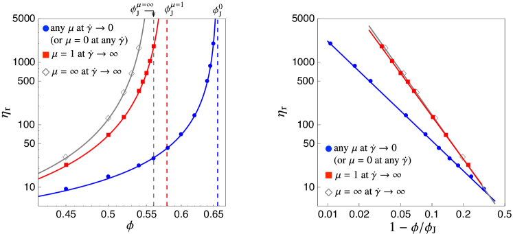
Figure 1: Relative viscosity $\eta_{\mathrm{r}}$ as a function of the volume fraction $\phi$ in the two limits $\dot{\gamma}\to 0$ and $\dot{\gamma}\to\infty$ (left). The $\dot{\gamma}\to 0$ viscosity (blue circles) is independent of the friction coefficient $\mu$ as the friction is not activated at low stresses, which leads to a relatively lower viscosity diverging at a higher volume fraction $\phi_{\mathrm{J}}^{0}$ (which is the jamming point for frictionless systems). The $\dot{\gamma}\to\infty$ viscosity however directly depends on $\mu$, as is seen from the difference between $\mu=1$ (red squares) and $\mu=\infty$ (gray diamonds) plots. In particular, the jamming volume fraction decreases with increasing $\mu$. We fit our data with power laws $\eta_{\mathrm{r}}=C(1-\phi/\phi_{\mathrm{J}})^{-\lambda}$ (right). The best fitting parameters are $(\phi_{\mathrm{J}}^{0},\lambda^{0},C^{0})\approx(0.66,1.6,1.40)$, $(\phi_{\mathrm{J}}^{\mu=1},\lambda^{\mu=1},C^{\mu=1})\approx(0.58,2.3,0.71)$, and $(\phi_{\mathrm{J}}^{\mu=\infty},\lambda^{\mu=\infty},C^{\mu=\infty})\approx(0.56,2.4,0.63)$.

For the ERM, the situation is the same at high shear rates, but differs at low shear rates. While friction is not felt for $\dot{\gamma}\to 0$, as particles do not contact, the finite range of the repulsive potential creates a shear thinning behavior from which we could not obtain the low shear-rate limit $\eta(\phi,\dot{\gamma}\to 0)$. The shear thinning comes from the fact that the system behaves essentially as soft particles at low shear stresses, with an apparent size that includes the hard sphere and a part of the surrounding soft repulsive potential. Indeed, a simple force balance argument at the scale of a particle says that if a particle is subject to a driving shear force $\sigma a^{2}$, the minimum gap $h_{\mathrm{min}}$ between this particle and its neighbors will be such that $F_{\mathrm{R}}(h_{\mathrm{min}})\sim\sigma a^{2}$ (with the limitation that it must respect the geometrical constraint, i.e., $h_{\mathrm{min}}<\bigl{(}1-\phi/\phi_{\mathrm{J}}^{0}\bigr{)}^{1/3}$). Then, at this shear stress the minimum center-to-center distance between two particles is $2a(1+h_{\mathrm{min}}(\sigma)/2)$, which means that the particles have an apparent radius larger than the one of their hard core. The jamming transition of these effectively bigger frictionless particles is at an apparent packing fraction (that is, based on the apparent diameter) $\phi^{\prime}=\phi_{\mathrm{J}}^{\prime 0}\approx 0.66$, which corresponds to an actual packing fraction $\phi$ significantly lower than $\phi_{\mathrm{J}}^{\prime 0}$. Because of this low volume fraction jamming transition at $\dot{\gamma}=0$, the viscosity is larger than at finite (but small) $\dot{\gamma}$, leading to the shear thinning we observe. Such thinning is actually known to occur due to repulsive forces in charge stabilized suspensions [Krieger, 1972; Maranzano and Wagner, 2001a].

III.2 Shear thickening, continuous and discontinuous

We can switch from one rheology to the other by varying the shear rate. Physically, the transmitted stress increases as the shear rate increases, which triggers the formation of frictional contacts between particles. Thus, by increasing the shear rate, the viscosity interpolates between the frictionless and frictional rheology curves, which means we can observe shear thickening. All this should be a natural consequence of the existence of two distinct rheologies at $\dot{\gamma}=0$ and $\dot{\gamma}=\infty$. What we cannot anticipate a priori is the way in which the system switches from the low viscosity state to the high viscosity one: do we observe a Continuous Shear Thickening (CST) or a Discontinuous Shear Thickening (DST)?

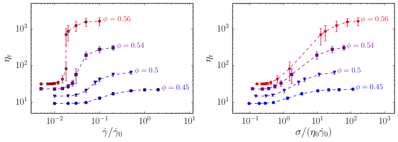
Figure 2: Shear rate $\dot{\gamma}$ (left) and shear stress $\sigma$ (right) dependences of the relative viscosity $\eta_{\mathrm{r}}$ for the critical load model (CLM), with friction coefficient $\mu=1$, for volume fractions $0.45\leq\phi\leq 0.56$. The system size is $N=1000$.

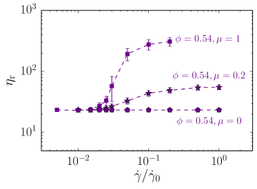
Figure 3: Effect of the friction coefficient $\mu$ on the shear rate dependence of the relative viscosity $\eta_{\mathrm{r}}(\dot{\gamma})$ in the CLM. The friction is essential to the shear thickening, as is illustrated by the reduction of the effect for $\mu=0.2$ and its complete suppression for $\mu=0$.

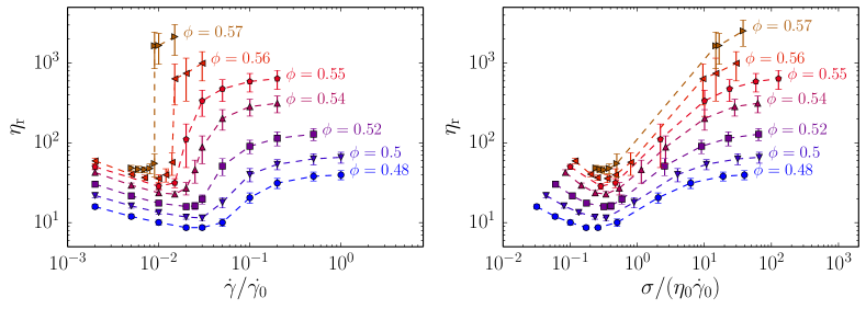
Figure 4: Shear rate $\dot{\gamma}$ (left) and shear stress $\sigma$ (right) dependences of the relative viscosity $\eta_{\mathrm{r}}$ for the electrostatic repulsion model (ERM), with friction coefficient $\mu=1$, for volume fractions $0.48\leq\phi\leq 0.57$. The system size is $N=512$.

The shear rate dependence of the viscosity, shown in Fig. 2 for the CLM, demonstrates the existence of both CST and DST in our system, depending on the volume fraction. As in experiments, when $\phi<\phi_{\mathrm{c}}$ the shear thickening is continuous, getting steeper and steeper as we approach $\phi_{\mathrm{c}}$, at which point it becomes discontinuous and keeps this behavior for $\phi>\phi_{\mathrm{c}}$ and up to $\phi_{\mathrm{J}}^{0}$. Note that there appears to be a real discontinuity in our data for these volume fractions: the time series of the viscosity show an intermittent behavior switching between two states, which we address in Sec. III.3. In Fig. 2, the intermittent data are split between low and high viscosity states: two points that correspond to a separate time average for each of the two states appear at the same shear rate.

When plotted against stress in Fig. 2, the viscosity curves show another interesting feature, namely that the onset of shear thickening occurs at a stress $\sigma_{\mathrm{ST}}/(\eta_{0}\dot{\gamma}_{0})\approx 0.3$ that is roughly independent of the volume fraction, as is observed in many experiments [Frith et al., 1996; Bender and Wagner, 1996; Maranzano and Wagner, 2001b, a; Lootens et al., 2005; Fall et al., 2010; Larsen et al., 2010; Brown and Jaeger, 2012, 2014]. Similarly, the transition towards the shear-rate independent plateau at high viscosity also occurs at a stress independent of $\phi$. The stress range over which thickening occurs remains constant from a mild shear thickening to a marked DST, as expected from a simple balance argument between the driving stress $\sigma=\eta\dot{\gamma}$ and the stress required to create a frictional contact $\sim F_{\mathrm{CL}}/a^{2}$ (for the CLM) with the area $a^{2}$ meaning that we require almost every particle to have a contact. It implies the thickening should roughly take place around $\sigma\approx F_{\mathrm{CL}}/a^{2}=6\pi\eta_{0}\dot{\gamma}_{0}$, which gives $\sigma/(\eta_{0}\dot{\gamma}_{0})\approx 6\pi$. This value falls at the upper end of the thickening regime as shown in Fig. 2, which is consistent with our assumption that at this stress scale every particle should have contacts with its neighbors, hence the system is in the frictional rheology state. The inverse argument applied to the onset stress $\sigma_{\mathrm{ST}}$ finds that the area $A_{\mathrm{ST}}$ over which one unit of critical load applies is $\sigma_{\mathrm{ST}}=F_{\mathrm{CL}}/A_{\mathrm{ST}}$, with $A_{\mathrm{ST}}\approx(7a)^{2}$. That means that at the onset of shear thickening, the contact chains must be sparsely distributed.

Friction is an essential ingredient for the shear thickening to occur, as is illustrated in Fig. 3, which shows the effect of a reduction of the friction coefficient on the $\eta_{\mathrm{r}}(\dot{\gamma})$ curve in the CST regime. If the friction is removed ($\mu=0$), the effect is completely suppressed (which is expected, as the threshold force scale $F_{\mathrm{CL}}$ disappears from the equations of motion for $\mu=0$, and the simulation is then rigorously the same for all $\dot{\gamma}$). If the friction is only reduced ($\mu=0.2$), the shear thickening is milder than with $\mu=1$ friction at the same volume fraction. In that case, the CST however becomes more pronounced and turns to DST when one increases the volume fraction, just as for the $\mu=1$ case.

The ERM shown in Fig. 4 behaves in a similar manner, only adding a shear thinning regime at low shear rates as discussed in the last paragraph of Sec. III.1.

III.3 Discontinuity and hysteresis

The existence of two distinct flowing states suggests that one might expect to observe a hysteresis associated with DST. It is thus remarkable that, aside from suspensions that are hysteretic at the microscopic level (with attractive interactions, for example, since once particles are aggregated under flow they stay aggregated upon cessation of the flow), there are very few experimental reports of hysteresis in systems showing DST (one of the best examples is provided by Bender and Wagner [1996]).

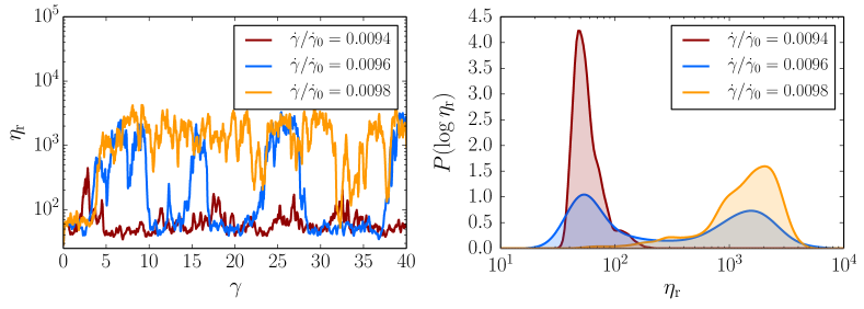
Figure 5: Strain (or dimensionless time) series of the shear stress close to the DST (left), and the corresponding histograms (right). The simulations are performed at $\phi=0.57$ with the ERM, with shear rates $\dot{\gamma}/\dot{\gamma}_{0}=0.0094$ (just below the DST region), $\dot{\gamma}/\dot{\gamma}_{0}=0.0096$ (in the DST region), and $\dot{\gamma}/\dot{\gamma}_{0}=0.0098$ (just above the DST region). Data at $\dot{\gamma}/\dot{\gamma}_{0}=0.0096$ show a superposition of the two states. This is very similar to what is seen in experiments [Boersma et al., 1991].

What is commonly observed, however, is a switching behavior, where the time series of the stress shows that the system shares its time between the two states, erratically switching in what looks like activated events [Boersma et al., 1991; D’Haene, Mewis, and Fuller, 1993; Bender and Wagner, 1996; Lootens, Van Damme, and Hébraud, 2003; Lootens et al., 2004, 2005; Hébraud and Lootens, 2005]. We observe this switching behavior in both models that we studied. In Fig. 5 we show time series of the stress and the corresponding histograms around the DST. These data show a typical “coexistence” behavior: significantly below and above shear thickening, the system respectively stays in the low and high viscosity state, but close to DST, the two states coexist in the same time series, the proportion of time spent in the high viscosity state increasing with $\dot{\gamma}$. While it is tempting to use the analogy of DST with an equilibrium first-order transition to conclude that the switchings are finite-size “activated” events, we need to be careful in doing so, because intermittency seems to survive for unusually large numbers of particles. The intermittency is still present in simulations with $N=1000$ particles, and the switching frequency does not seem to decrease relative to simulations with $N=512$ particles, whereas in a first order thermodynamic transition, one would expect the switching rate to be drastically reduced by a doubling of the system size. In fact, this effect might persist for much larger particle numbers, as is suggested by the experimentally observed intermittency [Boersma et al., 1991; D’Haene, Mewis, and Fuller, 1993; Bender and Wagner, 1996; Lootens, Van Damme, and Hébraud, 2003; Lootens et al., 2004, 2005; Hébraud and Lootens, 2005] in systems where $N$ is considerably larger. The simulations of Heussinger [2013] also show intermittency for systems of several thousands of particles. Moreover, should this phenomenon disappear in the thermodynamic limit, the fact that this limit is not observed until there are very large numbers of particles might be valuable information about the nature of this out-of-equilibrium phase transition, just as strong finite-size effects have a profound physical significance near a critical point.

In order to observe hysteresis one must have a system where the relaxation time $\tau_{\mathrm{relax}}$ (the length of the transient) is much smaller than the activation time $\tau_{\mathrm{act}}$ (the typical time between two switches). One then does a proper measurement with a shear rate sweep on a time scale $\tau_{\mathrm{sw}}$ such that $\tau_{\mathrm{relax}}\ll\tau_{\mathrm{sw}}\ll\tau_{\mathrm{act}}$: the first inequality ensures that the system is always in a steady state during the sweep and that the measurement is done with sufficient time averaging, while the second inequality ensures that we are not averaging data over two distinct states. In our simulations, as can be seen by looking at the time series in Fig. 5, a clear separation of time scales is not achieved (we have $\tau_{\mathrm{relax}}\lesssim\tau_{\mathrm{act}}$, which does not permit finding a proper $\tau_{\mathrm{sw}}$) and hysteresis cannot be observed unambiguously. Many experimental data actually suffer from the same limitations, and this might be the reason for the very small number of hysteretic flow curves actually reported. One exception is the noted work of Bender and Wagner [1996].

III.4 Normal stresses

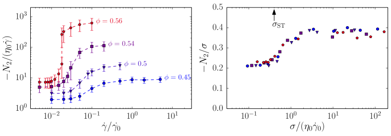
Figure 6: Shear rate dependence of the normalized second normal stress difference $N_{2}/\eta_{0}\dot{\gamma}$ (left) and shear stress dependence of $N_{2}/\sigma$ (right) for the CLM. The stress $\sigma_{\mathrm{ST}}$ at which thickening starts is marked by an arrow.

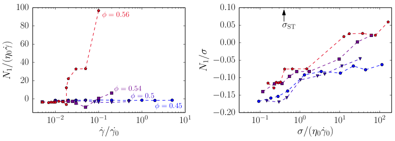
Figure 7: Shear rate dependence of the normalized first normal stress difference $N_{1}/\eta_{0}\dot{\gamma}$ (left) and shear stress dependence of $N_{1}/\sigma$ (right) for the CLM.

One common rheological characteristic of dense suspensions is the appearance of finite normal stress differences. Our measurements of the two normal stress differences $N_{1}$ and $N_{2}$ are shown in Fig. 7 and Fig. 6 for the CLM. The ERM behaves very similarly and is not shown.

We obtain for $N_{2}$ a behavior consistent with most experimental data available: it is negative, comparable to the shear stress (and much larger than $N_{1}$ that we discuss in the next paragraph), and its behavior is reminiscent of that of the shear stress. This comes from the fact that most of the stress is transmitted by forces in the shear plane (flow-gradient), not along the vorticity direction. Indeed the ratio $N_{2}/\sigma$ is rather insensitive to the stress magnitude, increasing at most by a factor of two across shear thickening while the stresses increase by almost two orders of magnitude. What is remarkable is the independence of $N_{2}/\sigma$ on the volume fraction: all volume fractions investigated here collapse on a master curve for both models.

There has been debate in the community regarding the value (and even the algebraic sign) of $N_{1}$. The first notable feature of our data concerning $N_{1}$ is that it is dominated by the fluctuations. In one time series, a cursory look indicates that its value fluctuates around zero. Long time averaging reveals more structure, however, as shown in Fig. 7 for the CLM. Prior to shear thickening, the average value of $N_{1}$ is nearly zero (slightly negative for CLM, slightly positive for ERM). The shear thickening transition is marked by two different behaviors, depending on the volume fraction: at the lowest volume fractions studied, $N_{1}$ decreases across shear thickening, while at larger $\phi$ there is a clear upturn towards positive values at the shear thickening transition. For the CLM, the behavior can be systematized by plotting $N_{1}$ as a function of the stress, as in Fig. 7: $N_{1}/\sigma$ is an increasing function of $\sigma$, negative at low stresses, with a qualitative behavior roughly independent of $\phi$. The same plot for the ERM is similar but less systematic. In any case, even above shear thickening, the ratio $N_{1}/\sigma$ is always small, never exceeding $0.1$.

Overall, the behavior we observe for $N_{1}$ is in reasonable agreement with most experiments [Lootens et al., 2005; Lee et al., 2006; Larsen et al., 2010; Couturier et al., 2011; Dbouk, Lobry, and Lemaire, 2013]. Zarraga, Hill, and Leighton [2000]; Singh and Nott [2003]; Dai et al. [2013] report a negative value for $N_{1}$. Lee et al. [2006] agree with our trend at low shear rates but observe a subsequent change towards negative $N_{1}$ at very high shear rates, while Dbouk, Lobry, and Lemaire [2013] find a positive but significantly larger $N_{1}$. In any case the amplitude of the fluctuations seems to be the relevant physical information about $N_{1}$, as the average, positive or negative, is buried in the fluctuations in the time series, such that at any time $N_{1}$ can be either positive or negative, even at large $\phi$ and $\dot{\gamma}$.

III.5 Microstructure

Non-Newtonian behavior of Brownian suspensions is often discussed with shear induced microstructure; the particle configuration is nearly at equilibrium at low Péclet number, while an anisotropic microstructure is induced by shear at high Péclet number [Morris, 2009]. Ideas associated with the order-disorder transition scenario [Hoffman, 1972, 1974, 1998] also predicted a clear structural change with shear thickening. Experimental observations, however, revealed that the low viscosity state was not always ordered and that the shear thickening can occur with only a subtle signature in the microstructure [Bender and Wagner, 1996; Watanabe et al., 1997, 1998; Newstein et al., 1999; Maranzano and Wagner, 2002]. One suggestion comes from the hydroclustering scenario, which assumes the existence of hydrodynamically created extended density fluctuations. Some experimental data are indeed in qualitative agreement with this scenario [Maranzano and Wagner, 2002; Cheng et al., 2011].

In the scenario we suggest in this article, the main structural modifications across the shear thickening transition should be sought in the contacts between particles. At low shear rates, frictional contacts are avoided because the particle pressure is too small to overcome the threshold (for the CLM) or the repulsion between particles (for the ERM). Those changes should thus be detected by measures specifically sensitive to the contacts. The pair correlation function should show few dramatic modifications across shear thickening. This is what we show in this section.

We define the pair correlation function:

$$g_{\mathrm{all}}(\bm{r})\equiv\frac{V}{N^{2}}\sum_{i,j}\delta(\bm{r}-\bm{r}_{ij}).$$ (13)

The system being bidisperse, we can also define partial pair correlation functions restricted to, e.g., pairs of small-small particles $g_{\mathrm{SS}}(\bm{r})\equiv(V/N_{\mathrm{S}}^{2})\sum_{i,j\in\mathcal{S}_{\mathrm{S}}}\delta(\bm{r}-\bm{r}_{ij})$ where $\mathcal{S}_{\mathrm{S}}$ is the subset of $N_{\mathrm{S}}$ small particles. In the same way, we define the structure factor (which is related to the pair correlation function via a Fourier Transform) as

$$S_{\mathrm{all}}(\bm{k})\equiv\frac{1}{N}\sum_{i,j\in\mathcal{S},i\neq j}e^{i\bm{k}.\bm{r}_{ij}}.$$ (14)

In Fig. 8 and Fig. 9 we show the pair correlation function restricted to the shear plane (velocity/gradient) at $\phi=0.57$ for four values of the shear rate: $\dot{\gamma}/\dot{\gamma}_{0}=0.005$, well below DST; $\dot{\gamma}/\dot{\gamma}_{0}=0.015$, just below DST; $\dot{\gamma}/\dot{\gamma}_{0}=0.02$, just above DST and $\dot{\gamma}/\dot{\gamma}_{0}=0.05$, well above DST. As expected, the evolution of those plots seems weak around DST. The main feature is a loss of contrast, unveiling a more isotropic structure above shear thickening.

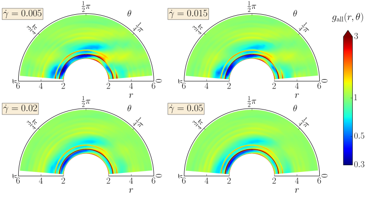
Figure 8: Pair correlation functions restricted in the shear plane $g_{\mathrm{all}}(r,\theta)$ for the CLM at $\phi=0.56$. The four plots correspond to shear rates $\dot{\gamma}=0.005$ (well below DST), $\dot{\gamma}=0.015$ (just below DST), $\dot{\gamma}=0.02$ (just above DST), and $\dot{\gamma}=0.05$ (well above DST).

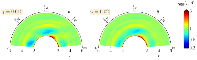
Figure 9: Pair correlation functions restricted to pairs of small particles in the shear plane $g_{\mathrm{SS}}(r,\theta)$ for the CLM at $\phi=0.56$. The two plots correspond to shear rates $\dot{\gamma}=0.015$ (just below DST) and $\dot{\gamma}=0.02$ (just above DST).

The structure factor shown in Fig. 10 reveals another interesting feature: there is a clear anisotropy in the shear plane in the low viscosity state, with a peak in the gradient direction that is strongly reduced (but not absent, see the right of Fig. 10) in the high viscosity state, above DST. This anisotropy is absent in the flow-vorticity plane; see Fig. 11. Looking back at the pair correlation functions in Fig. 8, we see that the peak of $S_{\mathrm{all}}(\bm{k})$ along the gradient direction is the signature of a slight ordering of the low viscosity phase: there are small but visible downstream ripples aligned with the flow direction at small shear rate.

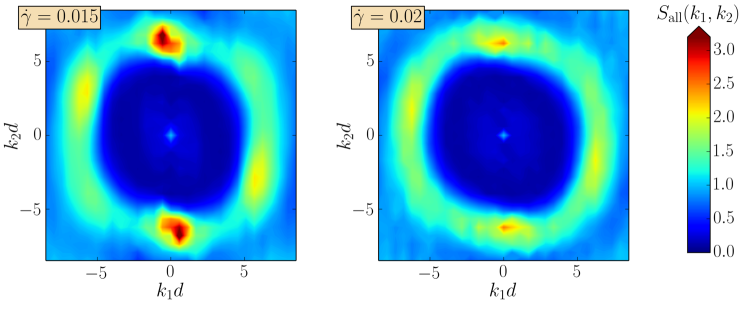
Figure 10: Structure factor in the shear plane $S_{\mathrm{all}}(k_{1},k_{2})$ for the CLM at $\phi=0.56$. Left: $\dot{\gamma}=0.015$ (just below DST). Right: $\dot{\gamma}=0.02$ (just above DST). The low viscosity state shows a peak in the gradient direction (around $k_{1}\approx 2\pi/d$) associated with a small amount of layering, which is strongly attenuated in the high viscosity phase.

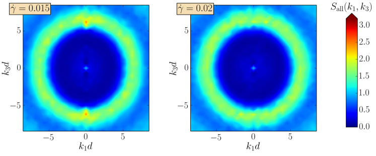
Figure 11: Structure factor in the flow-vorticity plane $S_{\mathrm{all}}(k_{1},k_{3})$ for the CLM at $\phi=0.56$. Left: $\dot{\gamma}=0.015$ (just below DST). Right: $\dot{\gamma}=0.02$ (just above DST). In this plane, the structure is isotropic in both states.

The slight layering we observe is however quite far from the string order usually associated with the order-disorder scenario. In the Supplementary Material, we show movies of the system projected on the gradient-vorticity plane (i.e., looking down the stream direction) for shear rates just below and just above shear thickening, where we reduced the size of the particles to a third of their actual radius to allow a better visualization. Those movies show warped layers along the flow-vorticity plane in some parts of the system, while in other parts ordered layers are completely absent. In any case, there is no further string ordering within the layers. This is consistent with our structure factor data in the gradient-vorticity direction (not shown), which exhibits only some structure in the gradient direction and no six-fold symmetry patterns typically observed when string ordering takes place [Laun et al., 1992; Kulkarni and Morris, 2009].

IV Discussion

IV.1 Contact network

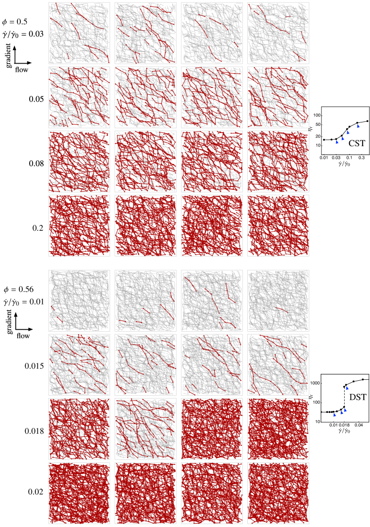
Figure 12: Snapshots of the contact network for the CLM at $\phi=0.5$ (top) and $0.56$ (bottom). Frictionless contacts (with normal force below the threshold $F_{\mathrm{CL}}$ are drawn in gray segments joining the centers of the two involved particles, while frictional contacts are drawn in red. Each row corresponds to a single shear rate, ranging from the low viscosity state to the high viscosity state and across CST (top) and DST (bottom). For each shear rate, we show four snapshots at different times (or equivalently strains) along the same simulation.

In our simulation, the shear thickening transition is due to the appearance of a growing number of frictional contacts as the shear rate (or more precisely the shear stress) increases. The contact network that is built across shear thickening is shown in Fig. 12 for the CLM for the two cases of CST and DST, respectively. (Two movies showing $\dot{\gamma}/\dot{\gamma}_{0}=0.015$ and $0.018$ of DST are available in the Supplementary Material. The time in these movies is scaled with $1/\dot{\gamma}$.)

At low shear rate, in the low viscosity state, frictional contacts only seldomly appear, being concentrated in small force chains along the compressional axis. At high shear rate, frictional contacts are the norm, creating a frictional contact network that is very close to being jammed; i.e., having only a few (collective) degrees of freedom left to reorganize under the applied stress.

Between those two extreme situations, a whole continuum of gradually denser frictional contact networks is seen across the CST transition in Fig. 12 (top). But in the case of DST in Fig. 12 (bottom), the contact network discontinuously changes from sparse to dense at the transition, never showing configurations of intermediate densities. Another interesting point is the occurrence of intermittency in the contact network, which is the immediate structural origin of the intermittent stress behavior shown in Fig. 5: close to DST, the contact network suddenly switches from mostly frictionless to mostly frictional, showing a large sensitivity to fluctuations. When this happens, the viscosity immediately follows by switching to high/low viscosity when the contact network respectively densifies/loosens.

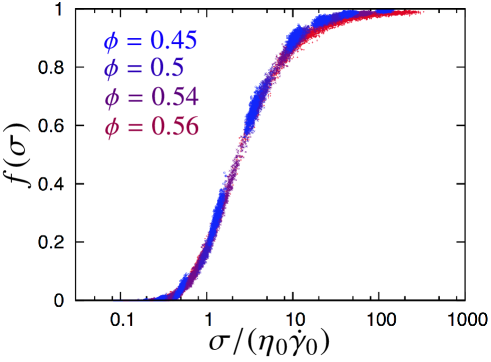
Figure 13: The fraction of frictional contacts $f$ as a function of the shear stress $\sigma$, for several volume fractions. There is a direct relation between the stress and the proportion of frictional contacts, which emphasizes the fundamental role of friction in shear thickening.

We can make the link between frictional contacts and shear stress explicit by looking at the fraction of frictional contacts $f$ [Wyart and Cates, 2014]. This quantity is unambiguously defined in the CLM model as the ratio of the number of contacts $N_{\mathrm{C}}^{\mathrm{f}}$ that are in the frictional state (those for which the normal force exceeds the critical load $F_{\mathrm{CL}}$) divided by the total number of contacts $N_{\mathrm{C}}$. This ratio has a direct relation to the shear stress, as the function $f(\sigma)$ plotted in Fig. 13 shows. This single relation demonstrates that, more than structural aspects, the shear thickening is above all a manifestation of the proliferation of frictional contacts in the system. We note one remarkable aspect of the relation $f(\sigma)$: it is independent of the volume fraction, at least in the range of $\phi$ that we have studied (which is rather large, owing to the fact that it should be understood as a range of distance to jamming $\phi-\phi_{\mathrm{J}}^{\mu}$ rather than a bare range of $\phi$). This peculiar aspect will be studied in a separate article.

IV.2 Phase diagram, relation to jamming

While the jamming transition is the critical phenomenon underlying DST, it should be noted that the jamming transition and DST are distinct, and in particular $\phi_{\mathrm{c}}\neq\phi_{\mathrm{J}}^{\mu}$. According to a recent theoretical argument by Wyart and Cates [2014], a scenario based on two diverging rheologies like the one we present in this work implies under reasonable assumptions that $\phi_{\mathrm{c}}<\phi_{\mathrm{J}}^{\mu}$; i.e., DST could then occur between two flowable (unjammed) states for volume fractions $\phi_{\mathrm{c}}<\phi<\phi_{\mathrm{J}}^{\mu}$.

In our simulations, we estimate $\phi_{\mathrm{J}}^{\mu=1}\approx 0.58$ (see Fig. 1), while we observe DST for $\phi=0.56$ (see Fig. 2), which indeed implies $\phi_{\mathrm{c}}<\phi_{\mathrm{J}}^{\mu=1}$. For a volume fraction $\phi>\phi_{\mathrm{J}}^{\mu=1}$ only the low viscosity state would be visible under shear, because the high viscosity frictional system is jammed at this volume fraction. This sets a maximum shear rate for the shear of the system at this volume fraction.

Physically, the two qualitatively different behaviors CST and DST, and the fact that $\phi_{\mathrm{c}}<\phi_{\mathrm{J}}^{\mu=1}$ can be explained in our model as stemming from the level of contrast that exists between frictionless and frictional rheologies, as suggested by Wyart and Cates [2014] (part of this explanation, when the contrast is diverging, was also suggested by Nakanishi, Nagahiro, and Mitarai [2012]). Recalling that the fraction of frictional contacts $f(\sigma)$ essentially depends only on the applied shear stress (see the previous Sec. IV.1), and noting that the viscosity interpolates between the two rheologies according to the number of frictional contacts, we see that we can write a direct relation $\eta(\sigma)$ between the viscosity and the applied stress. If the difference between the two rheologies is small—i.e., $\eta(\sigma\to\infty)-\eta(\sigma\to 0)$ is small—the curve $\eta(\sigma)$ is a sufficiently mildly increasing function such that $\dot{\gamma}=\sigma/\eta(\sigma)$ is also an increasing function of $\sigma$; this corresponds to a single-valued curve $\sigma(\dot{\gamma})$, and thus to CST. But if the difference $\eta(\sigma\to\infty)-\eta(\sigma\to 0)$ becomes too large, $\eta(\sigma)$ increases faster than $\sigma$ in some interval, which means that $\dot{\gamma}(\sigma)$ is a decreasing function in this same interval. This corresponds to a multivalued curve $\sigma(\dot{\gamma})$, which is unstable, and shows up experimentally as a discontinuous curve, i.e., DST.

An increasing difference $\eta(\sigma\to\infty)-\eta(\sigma\to 0)$ is naturally provided in our model by the fact that the frictional rheology diverges at a jamming volume fraction $\phi_{\mathrm{J}}^{\mu}$ that is smaller than the frictionless rheology jamming point $\phi_{\mathrm{J}}^{0}$. Then, at low volume fraction, the difference is small, but there must be a point $\phi_{\mathrm{c}}$ below $\phi_{\mathrm{J}}^{\mu}$ where the difference becomes large enough to observe a DST.

These ideas can be summed up in a phase diagram. The rheology is essentially frictionless in the lower part of the diagram Fig. 14, as the stress is too small to activate friction between grains. This rheology diverges at the frictionless jamming point $\phi_{\mathrm{J}}^{0}$. The rheology is frictional in the upper part of the diagram, as friction is activated under the applied stress. This rheology diverges at the frictional jamming point $\phi_{\mathrm{J}}^{\mu}$ and thus shows a larger viscosity than the frictionless rheology. Thus two rheologies coexist on the shear rate-volume fraction plane. Those rheologies are separated by a shear thickening that is continuous for $\phi<\phi_{\mathrm{c}}$ and discontinuous for $\phi_{\mathrm{c}}<\phi<\phi_{\mathrm{J}}^{\mu}$.

The discontinuity is actually related to the coexistence of the two rheologies in the triangle delimited by a dashed line. In this region, we observe one consequence of the coexistence in the intermittency of the flow: the system switches from one state to the other through activation events, as is shown by the time series of the stress (see Fig. 5). For $\phi_{\mathrm{J}}^{\mu}<\phi<\phi_{\mathrm{J}}^{0}$, DST is strictly speaking no longer observed, as the high viscosity flowable state does not exist any more. In this region, DST is actually replaced by shear jamming [Bi et al., 2011]: if one applies a shear stress larger than $\sigma_{\mathrm{ST}}$, the system goes to a solid state and cannot flow. This implies the existence of a forbidden region, in gray, where no flow is possible for hard spheres. In the lower shear-rate domain above $\phi_{\mathrm{J}}^{\mu}$, the low viscosity state is stable, but the activated events responsible for the intermittency at lower $\phi$ in small systems might lead to complete jamming in a finite time. Lastly, the dot in the upper left corner of the DST region is a critical point separating CST from DST. It shares some features with a critical point of a second order phase transition, for instance a diverging susceptibility $\mathrm{d}\sigma/\mathrm{d}\dot{\gamma}$.

Of course, as we numerically work with a shear-rate controlled scheme, the system always flows at any shear rate and any volume fraction, even in the forbidden region of the phase diagram. But in the latter region flow is only achieved by creating large overlaps between the particles (i.e., compressing them), hence violating the criteria we set to mimic hard sphere suspensions. At high shear rate and for $\phi>\phi_{\mathrm{J}}^{\mu}$, a real hard sphere system would not flow, but it does in the simulation because of our inability to enforce the hard sphere condition in a high (possibly infinite) stress state. The spheres we simulate in that case cannot be considered hard any more, and their stiffness sets a cutoff to the stress scales under shear. This situation is somehow similar to the one observed in experiments, where it is observed that the stress in the high viscosity state is set by the weakest stress scale in the sample (which might be a large stress scale for the rheometer usage range), whether it is the particles’ stiffness or the surface tension on the edge of the rheometer [Brown and Jaeger, 2012]. Therefore, in an experiment, even if the idealized system would be jammed under the investigated conditions, the real system still flows, perhaps thanks to dilation, whereas in our simulation, under the same conditions, it still flows thanks to the deformability of particles.

The difference between $\phi_{\mathrm{c}}$ and $\phi_{\mathrm{J}}^{\mu}$ may have been observed in some stress drop experiments [O’Brien and Mackay, 2000; Larsen et al., 2010]. For $\phi_{\mathrm{c}}<\phi<\phi_{\mathrm{J}}^{\mu}$, the phase diagram of Fig. 14 predicts that the stress in the thickened state would relax quickly upon flow cessation, as the contact network is unjammed. By contrast, for $\phi_{\mathrm{J}}^{\mu}<\phi<\phi_{\mathrm{J}}^{0}$ the stress would not relax entirely, as part of it would be stored elastically in the jammed contact network. This scenario is actually consistent with the data from [O’Brien and Mackay, 2000; Larsen et al., 2010].

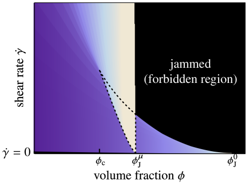
Figure 14: Schematic phase diagram in the shear rate-volume fraction plane. The viscosity is color coded, from small (dark blue) to large values (white). Along the $\phi$ axis, $\phi_{\mathrm{c}}$ is the point above which we can observe DST, $\phi_{\mathrm{J}}^{\mu}$ is the jamming point for frictional spheres with friction coefficient $\mu$, and $\phi_{\mathrm{J}}^{0}$ is the jamming point for frictionless spheres. Intermittency is observed in the region delimited by a dashed line.

V Conclusion

We have introduced a frictional-viscous model of dense suspensions under shear that is built on the framework used by previous standard models of suspensions: simulations are performed in the zero particle-inertia and zero fluid-inertia limits ($\mbox{{St}}\to 0$ and $\mbox{{Re}}\to 0$), and include relevant hydrodynamic interactions and a short-range repulsive potential. The critical innovation is that, besides this purely hydrodynamic basis, it includes frictional contacts between solid particles. This model can be used to simulate sheared suspensions over a range of volume fractions, from mildly dense, where the short range hydrodynamic interactions dominate, to the jamming point, where contact forces dominate.

The effect of adding frictional contacts is striking at large volume fractions: tangential forces due to friction restrict microscopic rearrangements in the system, resulting in a large shear stress. The number of contacts created during the flow is the result of a competition between applied shear forces and the short-range repulsive forces. Therefore, alongside the contactless (hence frictionless) rheology at low shear rates a new contact dominated frictional rheology appears at high shear rates. Shear thickening is then simply the transition from the contactless rheology to the contact dominated rheology with increasing shear stress (and shear rate). The strongest evidence that this stress-induced friction scenario is correct is the ability of our model to reproduce shear thickening, including its discontinuous form, and its volume-fraction dependence. Therefore, we conclude that friction is a key element for shear thickening.

The shear thickening mechanism we describe is qualitatively independent of our parameter choices. Quantitatively, we can summarize the effects of the various parameters as follows. The friction coefficient $\mu$ only affects the volume fraction range over which the phenomenon happens: if $\mu$ increases, the critical volume fraction $\phi_{\mathrm{c}}$ decreases. Any friction coefficient $\mu>0$ leads to a DST, with $\phi_{\mathrm{c}}(\mu)\to\phi_{\mathrm{J}}^{0}$ in the limit $\mu\to 0$. The lubrication cutoff $\delta$ mainly sets the dissipation level in the systems and thus sets an overall prefactor in the entire curve $\eta(\sigma)$: the viscosity is larger when $\delta$ decreases. For instance, we performed simulations with a cutoff $\delta=10^{-2}$ and compared the results to the ones shown in the present work obtained with $\delta=10^{-3}$: the curve $\eta^{\delta=10^{-2}}(\sigma)$ can be superimposed to $\eta^{\delta=10^{-3}}(\sigma)$ by a mere multiplicative factor $\eta^{\delta=10^{-2}}(\sigma)\approx 0.8\eta^{\delta=10^{-3}}(\sigma)$. This has the effect of pushing the shear thickening to lower shear rates, as the onset stress $\sigma_{\mathrm{ST}}$ is independent of $\delta$. The particle stiffness constants $k_{\mathrm{n}}$ and $k_{\mathrm{t}}$ are chosen such that the simulations are run in the asymptotic regime where the dimensionless numbers $6\pi\eta_{0}a\dot{\gamma}/k_{\mathrm{n,t}}$ are very small. In this asymptotic regime, the rheology is independent of these stiffness constants. The Debye length $\kappa^{-1}$ governs the shear thinning behavior at low shear rates. Our Critical Load Model can be thought as having a vanishing Debye length. Comparing with the Electrostatic Repulsion Model with $\kappa^{-1}=0.05a$ (with $a$ the radius of the small particles), we observe that besides the shear thinning regime, a finite $\kappa^{-1}$ virtually does not affect the shear thickening and the high viscosity state.

We now turn to a quantitative comparison with experimental data. The main tuning parameter in our description is the force scale $F_{\mathrm{CL}}$ for CLM (or $F_{\mathrm{ER}}$ for the ERM). This parameter sets the onset stress at which shear thickening occurs. We can estimate this force for a system of $1\text{\,}\mathrm{\SIUnitSymbolMicro m}$ silica spheres in water. We find an electrostatic repulsion at contact of order $F_{\mathrm{ER}}\approx$0.2\text{\,}\mathrm{nN}$$ (as evaluated in Behrens and Grier [2001] with a charge density $\approx$5\text{\times}{10}^{-4}\text{\,}\mathrm{C}\text{\,}{\mathrm{m}}^{-2}$$ and a Debye length $\kappa^{-1}\approx$0.1\text{\,}\mathrm{\SIUnitSymbolMicro m}$$). This gives for our model the stress scale $\eta_{0}\dot{\gamma}_{0}=(6\pi a^{2})^{-1}F_{\mathrm{ER}}$, which together with the non-dimensionalized onset stress $\sigma_{\mathrm{ST}}/(\eta_{0}\dot{\gamma}_{0})\approx 0.3$ obtained the ERM model (see Fig. 4) gives a predicted onset stress of $\sigma_{\mathrm{ST}}\approx$8\text{\,}\mathrm{Pa}$$. For the very same system, Lootens et al. [2005] experimentally find an onset stress of $\sigma_{\mathrm{ST}}\approx$5\text{\,}\mathrm{Pa}$$, with which our simulation is thus in good agreement. Thus, our mechanism seems to give a quantitative description of shear thickening in dense suspensions, even if it would require comparison to more experimental data to be definitely conclusive. (Obtaining a reliable value of the microscopic force scale is rarely feasible in the published data on DST, and this restricts the number of comparisons we can make at the moment.)

Although our model assumes non-Brownian suspensions, we may expect that the same mechanism explains shear thickening of Brownian colloidal suspensions. Indeed, the Brownian forces qualitatively play a role similar to the repulsive potential that we use in our ERM: at low shear stress, the Brownian forces are large enough to randomly open gaps between contacting particles, while at high shear stress this becomes much less likely, as relative trajectories of pairs of particles become smooth at high Peclet numbers [Nazockdast and Morris, 2013]. The fact that a random noise can relax friction between grains is a known phenomenon in granular matter [Gao et al., 2009; Karim and Corwin, 2014]. Friction would then develop in a Brownian suspension in a manner very similar to the present work.

Softwares and scripts

The code used to generate the data is available at https://bitbucket.org/rmari/lf_dem. Our code makes use of the CHOLMOD library v2.0.1 by Tim Davis (https://www.cise.ufl.edu/research/sparse/cholmod/) for direct Cholesky factorization of the sparse resistance matrix. Part of the data analysis and figure plotting was done using numpy v1.8.0, matplotlib v1.3.1 and IPython v1.1.0. The associated data and the IPython notebook are available at https://github.com/rmari/Data_Paper_JOR_58_1693_2014. The notebook can be visualized without IPython at http://nbviewer.ipython.org/github/rmari/Data_Paper_JOR_58_1693_2014/blob/master/JOR_figures_Rheology_Data.ipynb.

Appendix A Hydrodynamic resistances

The hydrodynamic interactions arising from an imposed background flow and relative motions between nearby particles are given by

$$\begin{pmatrix}\bm{F}_{\mathrm{H}}\\ \bm{T}_{\mathrm{H}}\end{pmatrix}=-(\bm{R}_{\mathrm{Stokes}}+\bm{R}_{\mathrm{Lub}})\cdot\begin{pmatrix}\bm{U}-\bm{U}^{\infty}\\ \bm{\Omega}-\bm{\Omega}^{\infty}\\ \end{pmatrix}+\bm{R}^{\prime}_{\mathrm{Lub}}:\bm{E}^{\infty},$$ (15)

where a diagonal matrix $\bm{R}_{\mathrm{Stokes}}$ comes from the (one-body) Stokes drag and sparse matrices $\bm{R}_{\mathrm{Lub}}$ and $\bm{R}^{\prime}_{\mathrm{Lub}}$ come from the (two-body) lubrication.

Using the basic units $L_{0}\equiv a$ for lengths, $U_{0}\equiv L_{0}\dot{\gamma}$ for velocities, and $F_{0}\equiv 6\pi\eta_{0}L_{0}U_{0}$ for forces, the elements of $\bm{R}_{\mathrm{Stokes}}$ give the Stokes drag through

$$\begin{pmatrix}\bm{F}_{\mathrm{Stokes}}^{(i)}\\ \bm{T}_{\mathrm{Stokes}}^{(i)}\end{pmatrix}=-\bm{R}^{(i,i)}_{\mathrm{Stokes}}\cdot\begin{pmatrix}\bm{U}^{(i)}-\bm{U}^{\infty}(\bm{r}^{(i)})\\ \bm{\Omega}^{(i)}-\bm{\Omega}^{\infty}\end{pmatrix}=-\begin{pmatrix}\bm{U}^{(i)}-\bm{U}^{\infty}(\bm{r}^{(i)})\\ (4/3)(\bm{\Omega}^{(i)}-\bm{\Omega}^{\infty})\end{pmatrix},$$ (16)

while $\bm{R}_{\mathrm{Lub}}$ and $\bm{R}^{\prime}_{\mathrm{Lub}}$ consist of off-diagonal blocks giving the lubrication forces and torques for a pair $(i,j)$ through

$$\left(\begin{array}{c}{𝑭}_{\mathrm{H}}^{(i,j)}\\ {𝑭}_{\mathrm{H}}^{(j,i)}\\ {𝑻}_{\mathrm{H}}^{(i,j)}\\ {𝑻}_{\mathrm{H}}^{(j,i)}\end{array}\right)=-{𝑹}_{\mathrm{Lub}}^{(i,j)}\cdot (\begin{array}{c}{𝑼}^{(i)}-{𝑼}^{\mathrm{\infty }}({𝒓}^{(i)})\\ {𝑼}^{(j)}\end{array}$$

References

- Andreotti, Barrat, and Heussinger [2012] Andreotti, B., Barrat, J.-L., and Heussinger, C., “Shear flow of non-brownian suspensions close to jamming,” Phys. Rev. Lett. 109, 105901 (2012).
- Bagnold [1954] Bagnold, R. A., “Experiments on a gravity-free dispersion of large solid spheres in a Newtonian fluid under shear,” Proc. R. Soc. Lond. A 225, 49–63 (1954).
- Ball and Melrose [1995] Ball, R. C. and Melrose, J. R., “Lubrication breakdown in hydrodynamic simulations of concentrated colloids,” Adv. Colloid Interface Sci. 59, 19–30 (1995).
- Ball and Melrose [1997] Ball, R. C. and Melrose, J. R., “A simulation technique for many spheres in quasi-static motion under frame-invariant pair drag and brownian forces,” Physica A 247, 444–472 (1997).
- Barnes [1989] Barnes, H. A., “Shear-thickening (“dilatancy”) in suspensions of nonaggregating solid particles dispersed in Newtonian liquids,” J. Rheol. 33, 329–366 (1989).
- Batchelor [1970] Batchelor, G. K., “The stress system in a suspension of force-free particles,” J. Fluid Mech. 41, 545–570 (1970).
- Behrens and Grier [2001] Behrens, S. H. and Grier, D. G., “The charge of glass and silica surfaces,” J. Chem. Phys. 115, 6716–6721 (2001).
- Bender and Wagner [1996] Bender, J. and Wagner, N. J., “Reversible shear thickening in monodisperse and bidisperse colloidal dispersions,” J. Rheol. 40, 899–916 (1996).
- Bender and Wagner [1995] Bender, J. W. and Wagner, N. J., “Optical measurement of the contributions of colloidal forces to the rheology of concentrated suspensions,” J. Colloid Interface Sci. 172, 171–184 (1995).
- Bertrand, Bibette, and Schmitt [2002] Bertrand, E., Bibette, J., and Schmitt, V., “From shear thickening to shear-induced jamming,” Phys. Rev. E 66, 060401 (2002).
- Bi et al. [2011] Bi, D., Zhang, J., Chakraborty, B., and Behringer, R. P., “Jamming by shear,” Nature 480, 355–358 (2011).
- Blanc, Peters, and Lemaire [2011] Blanc, F., Peters, F., and Lemaire, E., “Experimental signature of the pair trajectories of rough spheres in the shear-induced microstructure in noncolloidal suspensions,” Phys. Rev. Lett. 107, 208302 (2011).
- Boersma et al. [1991] Boersma, W. H., Baets, P. J. M., Laven, J., and Stein, H. N., “Time-dependent behavior and wall slip in concentrated shear thickening dispersions,” J. Rheol. 35, 1093–1120 (1991).
- Boersma, Laven, and Stein [1990] Boersma, W. H., Laven, J., and Stein, H. N., “Shear thickening (dilatancy) in concentrated dispersions,” AIChE J. 36, 321–332 (1990).
- Bossis and Brady [1989] Bossis, G. and Brady, J. F., “The rheology of brownian suspensions,” J. Chem. Phys. 91, 1866–1874 (1989).
- Boyer, Guazzelli, and Pouliquen [2011] Boyer, F., Guazzelli, É., and Pouliquen, O., “Unifying suspension and granular rheology,” Phys. Rev. Lett. 107, 188301 (2011).
- Brady and Bossis [1985] Brady, J. F. and Bossis, G., “The rheology of concentrated suspensions of spheres in simple shear flow by numerical simulation,” J. Fluid Mech. 155, 105–129 (1985).
- Brady and Bossis [1988] Brady, J. F. and Bossis, G., “Stokesian dynamics,” Ann. Rev. Fluid Mech. 20, 111–157 (1988).
- Brown and Jaeger [2009] Brown, E. and Jaeger, H. M., “Dynamic jamming point for shear thickening suspensions,” Phys. Rev. Lett. 103, 086001 (2009).
- Brown and Jaeger [2012] Brown, E. and Jaeger, H. M., “The role of dilation and confining stresses in shear thickening of dense suspensions,” J. Rheol. 56, 875–923 (2012).
- Brown and Jaeger [2014] Brown, E. and Jaeger, H. M., “Shear thickening in concentrated suspensions: phenomenology, mechanisms and relations to jamming,” Rep. Prog. Phys. 77, 046602 (2014).
- Cates et al. [1998] Cates, M. E., Wittmer, J. P., Bouchaud, J.-P., and Claudin, P., “Jamming, force chains, and fragile matter,” Phys. Rev. Lett. 81, 1841–1844 (1998).
- Cheng et al. [2011] Cheng, X., McCoy, J. H., Israelachvili, J. N., and Cohen, I., “Imaging the microscopic structure of shear thinning and thickening colloidal suspensions,” Science 333, 1276–1279 (2011).
- Couturier et al. [2011] Couturier, É., Boyer, F., Pouliquen, O., and Guazzelli, É., “Suspensions in a tilted trough: second normal stress difference,” J. Fluid Mech. 686, 26 (2011).
- Crawford et al. [2013] Crawford, N. C., Williams, S. K. R., Boldridge, D., and Liberatore, M. W., “Shear-induced structures and thickening in fumed silica slurries,” Langmuir 29, 12915–12923 (2013).
- Cundall and Strack [1979] Cundall, P. A. and Strack, O. D. L., “A discrete numerical model for granular assemblies,” Geotechnique 29, 47–65 (1979).
- da Cruz et al. [2005] da Cruz, F., Emam, S., Prochnow, M., Roux, J.-N., and Chevoir, F., “Rheophysics of dense granular materials: Discrete simulation of plane shear flows,” Phys. Rev. E 72, 021309 (2005).
- Dai et al. [2013] Dai, S.-C., Bertevas, E., Qi, F., and Tanner, R. I., “Viscometric functions for noncolloidal sphere suspensions with Newtonian matrices,” J. Rheol. 57, 493–510 (2013).
- Davis [1992] Davis, R. H., “Effects of surface roughness on a sphere sedimenting through a dilute suspension of neutrally buoyant spheres,” Phys. Fluids A 4, 2607–2619 (1992).
- Dbouk, Lobry, and Lemaire [2013] Dbouk, T., Lobry, L., and Lemaire, E., “Normal stresses in concentrated non-brownian suspensions,” J. Fluid Mech. 715, 239–272 (2013).
- Deboeuf et al. [2009] Deboeuf, A., Gauthier, G., Martin, J., Yurkovetsky, Y., and Morris, J. F., “Particle pressure in a sheared suspension: A bridge from osmosis to granular dilatancy,” Phys. Rev. Lett. 102, 108301 (2009).
- Denn and Morris [2014] Denn, M. M. and Morris, J. F., “Rheology of non-brownian suspensions,” Annu. Rev. Chem. Biomol. Eng. 5 (2014).
- D’Haene, Mewis, and Fuller [1993] D’Haene, P., Mewis, J., and Fuller, G. G., “Scattering dichroism measurements of flow-induced structure of a shear thickening suspension,” J. Colloid Interface Sci. 156, 350–358 (1993).
- Fagan and Zukoski [1997] Fagan, M. E. and Zukoski, C. F., “The rheology of charge stabilized silica suspensions,” J. Rheol. 41, 373–397 (1997).
- Fall et al. [2012] Fall, A., Bertrand, F., Ovarlez, G., and Bonn, D., “Shear thickening of cornstarch suspensions,” J. Rheol. 56, 575–591 (2012).
- Fall et al. [2010] Fall, A., Lemaître, A., Bertrand, F., Bonn, D., and Ovarlez, G., “Shear thickening and migration in granular suspensions,” Phys. Rev. Lett. 105, 268303 (2010).
- Fernandez et al. [2013] Fernandez, N., Mani, R., Rinaldi, D., Kadau, D., Mosquet, M., Lombois-Burger, H., Cayer-Barrioz, J., Herrmann, H. J., Spencer, N. D., and Isa, L., “Microscopic mechanism for shear thickening of non-brownian suspensions,” Phys. Rev. Lett. 111, 108301 (2013).
- Forterre and Pouliquen [2008] Forterre, Y. and Pouliquen, O., “Flows of dense granular media,” Annu. Rev. Fluid Mech. 40, 1–24 (2008).
- Foss and Brady [2000] Foss, D. R. and Brady, J. F., “Structure, diffusion and rheology of brownian suspensions by stokesian dynamics simulation,” J. Fluid Mech. 407, 167–200 (2000).
- Freundlich and Roder [1938] Freundlich, H. and Roder, H. L., “Dilatancy and its relation to thixotropy,” Trans. Faraday Soc. 34, 308–316 (1938).
- Frith et al. [1996] Frith, W. J., d’Haene, P., Buscall, R., and Mewis, J., “Shear thickening in model suspensions of sterically stabilized particles,” J. Rheol. 40, 531–548 (1996).
- Gao et al. [2009] Gao, G.-J., Blawzdziewicz, J., O’Hern, C. S., and Shattuck, M., “Experimental demonstration of nonuniform frequency distributions of granular packings,” Phys. Rev. E 80, 061304 (2009).
- Hébraud and Lootens [2005] Hébraud, P. and Lootens, D., “Concentrated suspensions under flow: shear-thickening and jamming,” Mod. Phys. Lett. B 19, 613–624 (2005).
- Heussinger [2013] Heussinger, C., “Shear thickening in granular suspensions: inter-particle friction and dynamically correlated clusters,” Phys. Rev. E 88, 050201(R) (2013).
- Ho and Tai [1998] Ho, C.-M. and Tai, Y.-C., “Micro-electro-mechanical-systems (mems) and fluid flows,” Annu. Rev. Fluid Mech. 30, 579–612 (1998).
- Hoffman [1972] Hoffman, R. L., “Discontinuous and dilatant viscosity behavior in concentrated suspensions. i. observation of a flow instability,” Trans. Soc. Rheol. 16, 155–173 (1972).
- Hoffman [1974] Hoffman, R. L., “Discontinuous and dilatant viscosity behavior in concentrated suspensions. ii. theory and experimental tests,” J. Colloid Interface Sci. 46, 491–506 (1974).
- Hoffman [1998] Hoffman, R. L., “Explanations for the cause of shear thickening in concentrated colloidal suspensions,” J. Rheol. 42, 111–123 (1998).
- Israelachvili [2011] Israelachvili, J. N., Intermolecular and surface forces (Academic Press, 2011).
- Jeffrey [1992] Jeffrey, D. J., “The calculation of the low reynolds number resistance functions for two unequal spheres,” Phys. Fluids A 4, 16–29 (1992).
- Jeffrey and Onishi [1984] Jeffrey, D. J. and Onishi, Y., “Calculation of the resistance and mobility functions for two unequal rigid spheres in low-reynolds-number flow,” J. Fluid Mech. 139, 261–290 (1984).
- Jerkins et al. [2008] Jerkins, M., Schröter, M., Swinney, H. L., Senden, T. J., Saadatfar, M., and Aste, T., “Onset of mechanical stability in random packings of frictional spheres,” Phys. Rev. Lett. 101, 018301 (2008).
- Karim and Corwin [2014] Karim, M. Y. and Corwin, E. I., “Eliminating friction with friction: 2d janssen effect in a friction-driven system,” Phys. Rev. Lett. 112, 188001 (2014).
- Kawasaki, Ikeda, and Berthier [2014] Kawasaki, T., Ikeda, A., and Berthier, L., “Thinning or thickening? multiple rheological regimes in dense suspensions of soft particles,” arXiv:1404.4778 [cond-mat] (2014).
- Krieger [1972] Krieger, I. M., “Rheology of monodisperse latices,” Adv. Colloid Interface Sci. 3, 111–136 (1972).
- Kulkarni and Morris [2009] Kulkarni, S. D. and Morris, J. F., “Ordering transition and structural evolution under shear in brownian suspensions,” J. Rheol. 53, 417–439 (2009).
- Larsen et al. [2010] Larsen, R. J., Kim, J.-W., Zukoski, C. F., and Weitz, D. A., “Elasticity of dilatant particle suspensions during flow,” Phys. Rev. E 81, 011502 (2010).
- Laun et al. [1992] Laun, H. M., Bung, R., Hess, S., Loose, W., Hess, O., Hahn, K., Hädicke, E., Hingmann, R., Schmidt, F., and Lindnerm, P., “Rheological and small angle neutron scattering investigation of shear-induced particle structures of concentrated polymer dispersions submitted to plane poiseuille and couette flow,” J. Rheol. 36, 743–787 (1992).
- Lee et al. [2006] Lee, M., Alcoutlabi, M., Magda, J. J., Dibble, C., Solomon, M. J., Shi, X., and McKenna, G. B., “The effect of the shear-thickening transition of model colloidal spheres on the sign of n1 and on the radial pressure profile in torsional shear flows,” J. Rheol. 50, 293–311 (2006).
- Lees and Edwards [1972] Lees, A. W. and Edwards, S. F., “The computer study of transport processes under extreme conditions,” J. Phys. C. 5, 1921 (1972).
- Lemaître, Roux, and Chevoir [2009] Lemaître, A., Roux, J.-N., and Chevoir, F., “What do dry granular flows tell us about dense non-brownian suspension rheology?” Rheol. Acta 48, 925–942 (2009).
- Lerner, Düring, and Wyart [2012] Lerner, E., Düring, G., and Wyart, M., “A unified framework for non-brownian suspension flows and soft amorphous solids,” Proc. Natl. Acad. Sci. USA 109, 4798–4803 (2012).
- Lootens et al. [2005] Lootens, D., van Damme, H., Hémar, Y., and Hébraud, P., “Dilatant flow of concentrated suspensions of rough particles,” Phys. Rev. Lett. 95, 268302 (2005).
- Lootens et al. [2004] Lootens, D., Hébraud, P., Lécolier, E., and Van Damme, H., “Gelation, shear-thinning and shear-thickening in cement slurries,” Oil Gas Sci. Technol.- Rev. IFP. 59, 31–40 (2004).
- Lootens, Van Damme, and Hébraud [2003] Lootens, D., Van Damme, H., and Hébraud, P., “Giant stress fluctuations at the jamming transition,” Phys. Rev. Lett. 90, 178301 (2003).
- Luding [2008] Luding, S., “Cohesive, frictional powders: contact models for tension,” Granular Matter 10, 235–246 (2008).
- Maranzano and Wagner [2001a] Maranzano, B. J. and Wagner, N. J., “The effects of interparticle interactions and particle size on reversible shear thickening: Hard-sphere colloidal dispersions,” J. Rheol. 45, 1205–1222 (2001a).
- Maranzano and Wagner [2001b] Maranzano, B. J. and Wagner, N. J., “The effects of particle size on reversible shear thickening of concentrated colloidal dispersions,” J. Chem. Phys. 114, 10514–527 (2001b).
- Maranzano and Wagner [2002] Maranzano, B. J. and Wagner, N. J., “Flow-small angle neutron scattering measurements of colloidal dispersion microstructure evolution through the shear thickening transition,” J. Chem. Phys. 117, 10291–302 (2002).
- Melrose and Ball [2004a] Melrose, J. R. and Ball, R. C., ““contact networks” in continuously shear thickening colloids,” J. Rheol. 48, 961–978 (2004a).
- Melrose and Ball [2004b] Melrose, J. R. and Ball, R. C., “Continuous shear thickening transitions in model concentrated colloids–the role of interparticle forces,” J. Rheol. 48, 937–960 (2004b).
- Metzner and Whitlock [1958] Metzner, A. B. and Whitlock, M., “Flow behavior of concentrated (dilatant) suspensions,” Trans. Soc. Rheol. 2, 239–253 (1958).
- Mewis and Wagner [2011] Mewis, J. and Wagner, N. J., Colloidal Suspension Rheology (Cambridge University Press, 2011).
- Morris [2009] Morris, J. F., “A review of microstructure in concentrated suspensions and its implications for rheology and bulk flow,” Rheol. Acta 48, 909–923 (2009).
- Nakanishi, Nagahiro, and Mitarai [2012] Nakanishi, H., Nagahiro, S., and Mitarai, N., “Fluid dynamics of dilatant fluids,” Phys. Rev. E 85, 011401 (2012).
- Nazockdast and Morris [2013] Nazockdast, E. and Morris, J. F., “Pair-particle dynamics and microstructure in sheared colloidal suspensions: Simulation and smoluchowski theory,” Phys. Fluids 25, 070601 (2013).
- Newstein et al. [1999] Newstein, M. C., Wang, H., Balsara, N. P., Lefebvre, A. A., Shnidman, Y., Watanabe, H., Osaki, K., Shikata, T., Niwa, H., and Morishima, Y., “Microstructural changes in a colloidal liquid in the shear thinning and shear thickening regimes,” J. Chem. Phys. 111, 4827–4838 (1999).
- O’Brien and Mackay [2000] O’Brien, V. T. and Mackay, M. E., “Stress components and shear thickening of concentrated hard sphere suspensions,” Langmuir 16, 7931–7938 (2000).
- O’Hern et al. [2003] O’Hern, C. S., Silbert, L. E., Liu, A. J., and Nagel, S. R., “Jamming at zero temperature and zero applied stress: The epitome of disorder,” Phys. Rev. E 68, 011306 (2003).
- Otsuki and Hayakawa [2011] Otsuki, M. and Hayakawa, H., “Critical scaling near jamming transition for frictional granular particles,” Phys. Rev. E 83, 051301 (2011).
- Phung, Brady, and Bossis [1996] Phung, T. N., Brady, J. F., and Bossis, G., “Stokesian dynamics simulation of brownian suspensions,” J. Fluid Mech. 313, 181–207 (1996).
- Seto et al. [2013] Seto, R., Mari, R., Morris, J. F., and Denn, M. M., “Discontinuous shear thickening of frictional hard-sphere suspensions,” Phys. Rev. Lett. 111, 218301 (2013).
- Silbert [2010] Silbert, L. E., “Jamming of frictional spheres and random loose packing,” Soft Matter 6, 2918–2924 (2010).
- Silbert et al. [2002] Silbert, L. E., Ertaş, D., Grest, G., Halsey, T. C., and Levine, D., “Geometry of frictionless and frictional sphere packings,” Phys. Rev. E 65, 1–6 (2002).
- Singh and Nott [2003] Singh, A. and Nott, P. R., “Experimental measurements of the normal stresses in sheared stokesian suspensions,” J. Fluid Mech. 490, 293–320 (2003).
- Song, Wang, and Makse [2008] Song, C., Wang, P., and Makse, H. A., “A phase diagram for jammed matter,” Nature 453, 629–632 (2008).
- Trulsson, Andreotti, and Claudin [2012] Trulsson, M., Andreotti, B., and Claudin, P., “Transition from the viscous to inertial regime in dense suspensions,” Phys. Rev. Lett. 109, 118305 (2012).
- Wagner and Brady [2009] Wagner, N. J. and Brady, J. F., “Shear thickening in colloidal dispersions,” Phys. Today 62, 27–32 (2009).
- Walton [1993a] Walton, O. R., “Numerical simulation of inclined chute flows of monodisperse, inelastic, frictional spheres,” Mech. Mater. 16, 239–247 (1993a).
- Walton [1993b] Walton, O. R., “Numerical simulation of inelastic, frictional particle-particle interactions,” (Butterworth-Heinemann, 1993) Chap. 25, pp. 884–911.
- Watanabe et al. [1997] Watanabe, H., Yao, M.-L., Osaki, K., Shikata, T., Niwa, H., and Morishima, Y., “Nonlinear rheology of a concentrated spherical silica suspension:,” Rheol. Acta 36, 524–533 (1997).
- Watanabe et al. [1998] Watanabe, H., Yao, M.-L., Osaki, K., Shikata, T., Niwa, H., Morishima, Y., Balsara, N. P., and Wang, H., “Nonlinear rheology and flow-induced structure in a concentrated spherical silica suspension,” Rheol. Acta 37, 1–6 (1998).
- Williamson [1930] Williamson, R. V., “Some unusual properties of colloidal dispersions,” J. Phys. Chem. 35, 354–359 (1930).
- Williamson and Hecker [1931] Williamson, R. V. and Hecker, W. W., “Some properties of dispersions of the quicksand type,” Ind. Eng. Chem. 23, 667–670 (1931).
- Wyart and Cates [2014] Wyart, M. and Cates, M. E., “Discontinuous shear thickening without inertia in dense non-brownian suspensions,” Phys. Rev. Lett. 112, 098302 (2014).
- Yurkovetsky and Morris [2008] Yurkovetsky, Y. and Morris, J. F., “Particle pressure in sheared brownian suspensions,” J. Rheol. 52, 141–164 (2008).
- Zarraga, Hill, and Leighton [2000] Zarraga, I. E., Hill, D. A., and Leighton, D. T., “The characterization of the total stress of concentrated suspensions of noncolloidal spheres in Newtonian fluids,” J. Rheol. 44, 185–220 (2000).
- Zhao and Davis [2002] Zhao, Y. and Davis, R. H., “Interaction of two touching spheres in a viscous fluid,” Chem. Eng. Sci. 57, 1997–2006 (2002).