Confidence intervals for high-dimensional inverse covariance estimation

Abstract

We propose methodology for statistical inference for low-dimensional parameters of sparse precision matrices in a high-dimensional setting. Our method leads to a non-sparse estimator of the precision matrix whose entries have a Gaussian limiting distribution. Asymptotic properties of the novel estimator are analyzed for the case of sub-Gaussian observations under a sparsity assumption on the entries of the true precision matrix and regularity conditions. Thresholding the de-sparsified estimator gives guarantees for edge selection in the associated graphical model. Performance of the proposed method is illustrated in a simulation study.

1 Introduction

A large number of methods has been proposed for the problem of inverse covariance estimation in high-dimensional settings, where the number of parameters may be much larger than the sample size. Common procedures in literature typically take advantage of thresholding which leads to estimators whose asymptotic distribution largely depends on the underlying unknown parameter [Knight and Fu [2000]] and is in general not tractable, which makes it challenging to establish any results for statistical inference. In this paper, motivated by the semi-parametric approach adopted in [van de Geer et al. [2013]] and [Zhang and Zhang [2014]], we propose an asymptotically normal non-sparse estimator of the precision matrix which leads to confidence regions and testing for low-dimensional parameters.

The problem of estimating the inverse covariance matrix in high dimensions naturally arises in a wide variety of application domains, such as graphical modeling of brain connectivity based on FMRI brain analysis [Ng, G. Varoquaux and Thirion [2013]], gene regulatory network discovery [Schäfer and Strimmer [2005]], financial data processing, social network analysis and climate data analysis. The development of methodology for high-dimensional inference is of interest for instance in differential networks, which comprise two sample comparisons of high-dimensional graphical models where the goal is to test equality of networks corresponding to two different populations. Differential networks find application e.g. in cancer studies [Städler and Mukherjee [2013]].

Consider an i.i.d. sample $X_{1},\dots,X_{n}\in\mathbb{R}^{p}$ of size $n$ from a zero-mean distribution with unknown covariance matrix $\Sigma^{*}\in\mathbb{R}^{p\times p}.$ Denoting the inverse covariance matrix, often referred to as the precision or concentration matrix, as $\Theta^{*}=(\Sigma^{*})^{-1},$ the goal is to the estimate $\Theta^{*}$ in a setting where $p\gg n.$ The most natural candidate for an estimator of the covariance matrix is presumably the sample covariance matrix. However, when $p>n$, the sample covariance matrix is singular with probability one. Even when $p/n$ tends to a constant, the covariance matrix exhibits poor performance [Johnstone [2001]].

Different structural assumptions have been imposed on the model to allow for consistent estimation in the regime $p\gg n$, here we consider in particular sparsity assumptions on the number of non-zero elements of the precision matrix. Let $\mathcal{V}:=\{1,\dots,p\}$, let $S\equiv S(\Theta^{*}):=\{(i,j)\in\mathcal{V}\times\mathcal{V}:\Theta^{*}_{ij}\not=0\}$ be the set of all non-zero entries of $\Theta^{*}$ and denote the cardinality of $S$ by $s.$ Use $S^{c}(\Theta^{*})$ for the complement of $S(\Theta^{*})$ in $\mathcal{V}\times\mathcal{V}.$ We shall impose a sparsity assumption on the maximum row cardinality of $\Theta^{*}$; therefore define $d=d_{n}$ as follows

$$d:=\max_{i\in\{1,\dots,p\}}|\{j\in\mathcal{V}:\Theta^{*}_{ij}\not=0\}|.$$

Estimation of precision matrices is of interest in Gaussian graphical modeling where the entries of the precision matrix represent conditional dependences between the variables [Lauritzen [1996]]. Suppose that $X=(X^{1},\dots,$ $X^{p})\sim\mathcal{N}(0,\Sigma^{*})$ and associate the variables $X^{1},\dots,X^{p}$ with the vertex set $\mathcal{V}=\{1,\dots,p\}$ of an undirected graph $\mathcal{G}=(\mathcal{V},\mathcal{E})$ with an edge set $\mathcal{E}.$ A pair $(i,j)$ is included in the edge set if and only if the variables $X^{i}$ and $X^{j}$ are not independent given all remaining variables. Under $X\sim\mathcal{N}(0,\Sigma^{*})$, a pair of variables is conditionally independent given all remaining variables if and only if the corresponding entry in the precision matrix $\Theta^{*}=(\Sigma^{*})^{-1}$ is zero. Hence a pair of variables is contained in the edge set if and only if the corresponding entry in the inverse covariance matrix $\Theta^{*}=(\Sigma^{*})^{-1}$ is non-zero ([Lauritzen [1996]]). Elements of the precision matrix may thus be interpreted as the edge weights in the Gaussian graphical model. The parameter $d$ corresponds to the maximum node degree in the associated Gaussian graphical model and thus sparsity assumptions on $d$ translate to sparsity of the edges in the graphical model.

1.1 Overview of related work

Existing work on statistical inference in high dimensional settings has mostly focused on inference for parameters in linear models and generalized linear models [van de Geer et al. [2013], Zhang and Zhang [2014], Meinshausen [2013], Javanmard and Montanari [2013a], Chatterjee and Lahiri [2013], Chatterjee and Lahiri [2011], Nickl and van de Geer [2012]]. In particular we mention the paper [Zhang and Zhang [2014]] where a semi-parametric projection approach was proposed for testing and construction of confidence intervals for low-dimensional parameters. The proposed method is based on the Lasso estimator for which the Karush-Kuhn-Tucker conditions are “inverted” to obtain a de-sparsified estimator. The approach leads to asymptotically normal and efficient (in a semi-parametric sense) estimation of the regression coefficients and an extension of the method to generalized linear models is given in [van de Geer et al. [2013]]. The key assumption which allows for asymptotically normal estimation requires sparsity of order $\sqrt{n}/\log p$ in the high-dimensional parameter vector and the method relies on $\ell_{1}$ norm error bound of the Lasso. The paper [Javanmard and Montanari [2013a]] essentially follows the same approach as [Zhang and Zhang [2014]] but uses a different approach to find an approximate inverse for the sample covariance matrix.

Further methodology for inference for the regression coefficients in high-dimensional regression includes methods based on sample splitting [Meinshausen, Meier and Bühlmann [2009], Wasserman and Roeder [2009]], bootstrapping approach [Chatterjee and Lahiri [2013], Chatterjee and Lahiri [2011]], inference after variable selection [Berk et al. [2013]] and other [Meinshausen [2013], Belloni, Chernozhukov and Hansen [2014]].

Estimation of precision matrices is a problem closely related to linear regression and in high dimensions has been extensively studied in terms of point estimation. Less work has yet been done on inference for precision matrices in this setting. We mention the work [Ren et al. [2013]] which suggests a regression approach leading to an asymptotically normal estimator for elements of the precision matrix, under row sparsity of order $\sqrt{n}/\log p$, bounded spectrum of the true precision matrix and Gaussianity of the underlying distribution. The procedure regresses each pair of variables $(X^{i},X^{j})$ on all the remaining variables for each $(i,j)\in\mathcal{V}\times\mathcal{V}$ to obtain an estimate of the noise level of the conditional distribution of $(X^{i},X^{j})$. This requires $\mathcal{O}(p^{2})$ high-dimensional regressions with the square-root Lasso ([Belloni, Chernozhukov and Wang [2011]]).

The large amount of work that has studied methodology for point estimation of precision matrices (a selected list includes [Friedman, Hastie and Tibshirani [2008], Meinshausen and Bühlmann [2006], Yuan [2010], Cai, Liu and Luo [2011], Sun and Zhang [2012], Bickel and Levina [2008]]) typically uses regularization in terms of $\ell_{1}$ norm or some sort of thresholding of the sample covariance matrix. Hence they do not immediately lead to results for inference, but we show they may serve as good initial estimators to construct asymptotically normal estimators.

Here we consider in particular the graphical Lasso, which minimizes the negative Gaussian log-likelihood with regularization in terms of the $\ell_{1}$ norm of the off-diagonal entries of the precision matrix and has been studied in detail in several papers [Friedman, Hastie and Tibshirani [2008], Rothman et al. [2008], Ravikumar et al. [2008]] and [Yuan and Lin [2007]]. The optimization problem corresponding to graphical Lasso is a convex optimization problem that can be solved with coordinate descent methods [d’Aspremont, Banerjee and El Ghaoui [2008], Friedman, Hastie and Tibshirani [2008]] in polynomial time.

The asymptotic behaviour of the graphical Lasso has been studied in [Rothman et al. [2008]] (see also [Negahban et al. [2010]]) which derives rates of convergence in Frobenius norm of order $O((p+d)\log p/n)$ under mild conditions on the eigenvalues of $\Theta^{*}$ and under sparsity $(p+d)\log p/n\rightarrow 0.$ High-dimensionality here is reflected in $p$ being allowed to grow as a function of $n$, however, in limit, $p/n\rightarrow 0$ is required. The high-dimensional setting $p\gg n$ is considered in [Ravikumar et al. [2008]], where convergence rates for the supremum norm of order $O(\kappa_{\Gamma^{*}}\sqrt{\log p/n})$ are derived under an irrepresentability condition on the true precision matrix $\Theta^{*}$, sparsity $d^{2}\log p/n\rightarrow 0$ and sub-Gaussian tails of the underlying distribution. The rates depend on certain quantities $\kappa_{\Gamma^{*}}$ and $\kappa_{\Sigma^{*}}$, where $\kappa_{\Gamma^{*}}$ is the $\ell_{1}$ matrix norm of the inverse of a certain subset of the Hessian matrix $\Gamma^{*}=\Sigma^{*}\otimes\Sigma^{*}$ and $\kappa_{\Sigma^{*}}$ the $\ell_{1}$ matrix norm of the true covariance matrix $\Sigma^{*}$. For reader’s convenience we discuss the results in more detail in Section 1.3 and appendix A.

Further methodology on estimation of precision matrices in particular includes the regression approach [Meinshausen and Bühlmann [2006], Yuan [2010], Cai, Liu and Luo [2011]] and [Sun and Zhang [2012]] which uses a Lasso-type algorithm or Dantzig selector [Candes and Tao [2007]] to estimate each column or a smaller part of the precision matrix individually, thresholding of the sample covariance matrix [Bickel and Levina [2008]] or a combination thereof.

1.2 Outline

In this paper, we propose a de-sparsified estimator based on the graphical Lasso and study its theoretical properties for low-dimensional statistical inference and edge selection in the associated graphical model. The work closely follows the approach of [van de Geer et al. [2013]], which builds on “inverting” the necessary Karush-Kuhn-Tucker conditions for an optimization problem. The paper [van de Geer et al. [2013]] demonstrates this method for the case of linear regression and generalized linear models, while we apply the idea to a fully nonlinear estimator. By inverting the KKT conditions, we obtain a de-sparsified graphical Lasso estimator and consequently we analyze its asymptotic properties. Asymptotic normality of the new estimator is proved for sub-Gaussian observations, under regularity conditions on the true precision matrix $\Theta^{*}$. The estimator may be thresholded again to give guarantees for edge selection in the associated graphical model. The performance of the method is illustrated on both simulated and real data.

The paper is organized as follows. In Section 1.3, we briefly introduce the model. Section 2 contains the main results. Section 3 illustrates the theoretical results in a simulation study and on a real data set. Finally, Section 4 contains proofs.

Notation. For two matrices $A$ and $B$, use $A\otimes B$ to denote the Kronecker product of $A$ and $B.$ For a vector $x\in\mathbb{R}^{d}$ and $p\in(0,\infty]$ we use the notation $\|x\|_{p}$ to denote the $p-$norm of $x$ in the classical sense. For a matrix $A\in\mathbb{R}^{d\times d}$ we use the notations ${\left|\kern-1.07639pt\left|\kern-1.07639pt\left|A\right|\kern-1.07639pt\right|\kern-1.07639pt\right|}_{\infty}=\max_{i}\|e_{i}^{T}A\|_{1}$, ${\left|\kern-1.07639pt\left|\kern-1.07639pt\left|A\right|\kern-1.07639pt\right|\kern-1.07639pt\right|}_{1}={\left|\kern-1.07639pt\left|\kern-1.07639pt\left|A^{T}\right|\kern-1.07639pt\right|\kern-1.07639pt\right|}_{\infty}$ and $\|A\|_{\infty}=\max_{i,j}|A_{ij}|$. The symbol $\text{vec}(A)$ denotes the vectorized version of a matrix $A$ obtained by stacking rows of $A$ on each other. By $e_{i}$ we denote a $p$-dimensional vector of zeros with one at position $i$ and by $e_{ij}:=e_{i}\otimes e_{j}$ a $p^{2}$-dimensional vector of zeros with one at position indexed by $(i,j).$

For sequences $f_{n},g_{n}$, we write $f_{n}=O(g_{n})$ if $|f_{n}|\leq C|g_{n}|$ for some $C>0$ independent of $n$ and all $n>C.$ Analogously, we write $f_{n}=\Omega(g_{n})$ if $|f_{n}|\geq C|g_{n}|$ for some $C>0$ independent of $n$ and all $n>C.$ We write $f_{n}\asymp g_{n}$ if both $f_{n}=\mathcal{O}(g_{n})$ and $f_{n}=\Omega(g_{n})$ hold. Finally, $f_{n}=o(g_{n})$ if $\lim_{n\rightarrow\infty}f_{n}/g_{n}=0.$

We use $S_{+}^{p}$ to denote the cone of positive semi-definite $p\times p$ matrices, i.e. $S_{+}^{p}:=\{A\in\mathbb{R}^{p\times p}|A=A^{T},A\succeq 0\}$ and $S^{p}_{++}$ to denote the set of positive definite $p\times p$ matrices, $S_{++}^{p}:=\{A\in\mathbb{R}^{p\times p}|A=A^{T},A\succ 0\}$.

The components of a vector $X\in\mathbb{R}^{p}$ will be denoted by upper indices, i.e. $X=(X^{1},\dots,X^{p})$. Elements of matrices will be typically denoted by lower indices, e.g. $A_{ij}.$ We use $\rightsquigarrow$ to denote convergence in distribution.

1.3 Model setup

Definition 1.

A real zero-mean random variable $X$ is sub-Gaussian if there exists $K>0$ such that

$$\mathbb{E}e^{X^{2}/K^{2}}\leq 2.$$ (1)

Condition (C1) implies a bound on the moment generating function $\mathbb{E}^{tX}\leq e^{\frac{3}{2}K^{2}t^{2}}$ for all $t>0$ and a tail bound $\mathbb{P}(|X|>t)\leq 2e^{-\frac{t}{6K^{2}}}$ for all $t>0,$ which are both equivalent characterizations of sub-Gaussianity. A prime example of a sub-Gaussian random variable is a zero-mean Gaussian random variable.

We shall consider the following sub-Gaussianity conditions for random vectors $X=(X^{1},\dots,X^{p})$ with zero mean and covariance matrix $\Sigma^{*}$.

Condition (C1) (Sub-Gaussianity condition).

All normalized components $X^{i}/\break\sqrt{\Sigma_{ii}^{*}},i=1,\dots,p$ of the zero-mean random vector $X=(X^{1},\dots,X^{p})$ with covariance matrix $\Sigma^{*}$ are sub-Gaussian random variables with a common parameter $K>0.$

The condition (C1) is weaker than requiring the sub-Gaussianity of the whole vector $X=(X^{1},\dots,X^{p})$ in the following sense.

Condition (C2) (Sub-Gaussianity vector condition).

A zero-mean random vector $X\in\mathbb{R}^{p}$ satisfies the sub-Gaussianity vector condition if there exists a constant $K>0$ such that

$$\sup_{\alpha\in\mathbb{R}^{p}:\|\alpha\|_{2}\leq 1}\mathbb{E}e^{|\alpha^{T}X|^{2}/K^{2}}\leq 2.$$ (2)

If a random vector $X=(X^{1},\dots,X^{p})$ satisfies (C2) with a constant $K$, then each component $X^{i}$ satisfies (1) with $K$.

We now review some notation and results related to the graphical Lasso estimator [Friedman, Hastie and Tibshirani [2008]] on which our further analysis is based. Consider an i.i.d. sample $X_{1},\dots,X_{n}$ distributed as $X$ with $\mathbb{E}X=0,\text{cov}(X)=\Sigma^{*}.$ Let $\hat{\Sigma}=\frac{1}{n}\sum_{i=1}^{n}X_{i}X_{i}^{T}$ be the sample covariance matrix. We further write $\hat{\Sigma}_{ij}:=(\hat{\Sigma})_{ij}$ for the $(i,j)$-th element of $\hat{\Sigma}$, $(i,j)\in\mathcal{V}\times\mathcal{V}$. The graphical Lasso estimator $\hat{\Theta}$ [Friedman, Hastie and Tibshirani [2008]] is defined as the solution to the optimization problem

$$\hat{\Theta}:=\text{arg}\min_{\Theta\in S_{++}^{p}}\left\{\text{trace}(\Theta^{T}\hat{\Sigma})-\log\text{det}(\Theta)+\lambda\|\Theta\|_{1,\text{off}}\right\},$$ (P1)

where $\hat{\Sigma}$ is the sample covariance matrix $\hat{\Sigma}=\frac{1}{n}\sum_{i=1}^{n}X_{i}X_{i}^{T}$ and $\|\cdot\|_{1,\text{off}}$ is the $\ell_{1}$ off-diagonal penalty, $\|\Theta\|_{1,\text{off}}=\sum_{i\not=j}|\Theta_{ij}|$. When the data is normally distributed, (P1) is equivalent to $\ell_{1}-$penalized maximum likelihood for the precision matrix.

In our analysis, we rely on the results on rates of convergence derived in [Ravikumar et al. [2008]] for the graphical Lasso in supremum norm. The work [Ravikumar et al. [2008]] assumes an irrepresentability condition which is a rather restrictive condition in the linear regression setting [van de Geer and Bühlmann [2009]]. However, other literature on the graphical Lasso [Yuan and Lin [2007]] likewise assumes irrepresentability condition or otherwise assumes $p/n\rightarrow 0$ [Rothman et al. [2008]]. In the linear regression setting, irrepresentable conditions are sufficient for variable selection [van de Geer and Bühlmann [2009], Meinshausen and Bühlmann [2006], Zhao and Yu [2006]].

The analysis of rates of convergence of the graphical Lasso in [Ravikumar et al. [2008]] in addition considers certain functions of the true precision matrix $\Theta^{*}$, which we now define.

Let $\kappa_{\Sigma^{*}}$ be the $\ell_{\infty}$ operator norm of the true covariance matrix $\Sigma^{*}$, i.e.

$$\kappa_{\Sigma^{*}}={\left|\kern-1.07639pt\left|\kern-1.07639pt\left|\Sigma^{*}\right|\kern-1.07639pt\right|\kern-1.07639pt\right|}_{\infty}=\max_{i}\sum_{j=1}^{p}|\Sigma^{*}_{ij}|.$$

The parameter $\kappa_{\Sigma^{*}}$ then measures the size of entries in $\Sigma^{*}$.

Example 1.

Consider the Töplitz matrix $\Sigma^{*}_{ij}=\rho^{|i-j|}$ for $i,j=1,\dots,p,$ where $|\rho|<1.$ Then $\kappa_{\Sigma^{*}}=({1-\rho^{p}})/{(1-\rho)}=\mathcal{O}(1)$ if $\rho$ is bounded away from $1$.

We next consider the Hessian $\Gamma(\Theta)$ of the negative log-likelihood function $\ell(\Theta)=\text{tr}(\Theta^{T}\hat{\Sigma})-\log\text{det}(\Theta)$. The entries of the gradient of $\ell$ are given by ([Greene [2011]])

$$\frac{\partial\ell(\Theta)}{\partial\Theta_{ij}}=\hat{\Sigma}_{ij}-(\Theta^{-1})_{ij}.$$

The Hessian matrix is then indexed by pairs of edges $((i,j),(k,l))$ and the $((i,j),(k,l))$-th entry takes the form

$$\frac{\partial^{2}\ell(\Theta)}{\partial\Theta_{kl}\partial\Theta_{ij}}=\frac{\partial(\hat{\Sigma}_{ij}-(\Theta^{-1})_{ij})}{\partial\Theta_{kl}\partial\Theta_{ij}}=e_{i}^{T}\Theta^{-1}e_{k}e_{l}^{T}\Theta^{-1}e_{j}=\Sigma_{ik}\Sigma_{lj},$$

where $\Sigma=\Theta^{-1}.$ In matrix form, we obtain

$$\Gamma(\Theta)=\Sigma\otimes\Sigma.$$

By $(i,j)$-th column of $\Sigma\otimes\Sigma$ we refer to the $p^{2}\times 1$ vector $\Sigma\otimes\Sigma\text{vec}(e_{i}e_{j}^{T})$ and $(i,j)$-th row of $\Sigma\otimes\Sigma$ is its transpose. The $(i,j)$-th row of $\Sigma\otimes\Sigma$ contains all mixed partial derivatives of $\ell$ with respect to $\Theta_{ij}$ and $\Theta_{kl}$ where $k,l=1,\dots,p$. Note that $\Theta\otimes\Theta$ may be viewed as a four-dimensional tensor.

We impose some restrictions on the Hessian $\Gamma$ evaluated at the true $\Theta^{*}$, $\Gamma^{*}:=\Gamma(\Theta^{*})$. To this end, let us fix the following notation. For any two subsets $T$ and $T^{\prime}$ of $\mathcal{V}\times\mathcal{V}$, we use $\Gamma^{*}_{TT^{\prime}}$ to denote the $|T|\times|T^{\prime}|$ matrix with rows and columns of $\Gamma^{*}$ indexed by $T$ and $T^{\prime}$ respectively.

Consequently, define $\kappa_{\Gamma^{*}}$ to be the $\ell_{\infty}$ operator norm of the inverse of the matrix

$$\Gamma_{SS}^{*}=[\Sigma^{*}\otimes\Sigma^{*}]_{SS}\in\mathbb{R}^{s\times s}.$$

i.e., $\kappa_{\Gamma^{*}}={\left|\kern-1.07639pt\left|\kern-1.07639pt\left|(\Gamma^{*}_{SS})^{-1}\right|\kern-1.07639pt\right|\kern-1.07639pt\right|}_{\infty}.$

The parameter $\kappa_{\Gamma^{*}}$ then measures the size of entries in $\Theta^{*}$ and assumptions on its growth are similar to sparsity assumptions on $\Theta^{*}$.

Example 2.

The parameter $\kappa_{\Gamma^{*}}$ is difficult to track in general as it involves inversion of a certain sub-matrix of the Hessian. A tractable example is the situation when $\Theta^{*}$ is a block diagonal matrix with blocks $B_{1},\dots,B_{k}$ for some $1\leq k\leq p$ which only contain non-zero (although possibly arbitrarily small) entries and the remaining off-diagonal entries of $\Theta^{*}$ are zero. Suppose that the sizes of the blocks are $b_{1},\dots,b_{k}$ and denote $d:=\max_{i=1,\dots,k}b_{i}.$ This corresponds to a graph with $k$ completely connected but mutually isolated subgraphs with maximum vertex degree $d.$ Using that block matrices can be easily inverted by inverting each block separately (and using that $(A\otimes A)^{-1}=A^{-1}\otimes A^{-1}$), some calculations give

$$\kappa_{\Gamma^{*}}=\max_{i=1,\dots,k}{\left|\kern-1.07639pt\left|\kern-1.07639pt\left|B_{i}\otimes B_{i}\right|\kern-1.07639pt\right|\kern-1.07639pt\right|}_{\infty}=\max_{i=1,\dots,k}{\left|\kern-1.07639pt\left|\kern-1.07639pt\left|B_{i}\right|\kern-1.07639pt\right|\kern-1.07639pt\right|}^{2}_{\infty}.$$

The size of $\kappa_{\Gamma^{*}}$ thus depends on the size of entries in $B_{i}^{\prime}s.$ We clearly have the upper bound

$$\kappa_{\Gamma^{*}}\leq d\max_{i=1,\dots,k}\max_{j=1,\dots,b_{i}}(B_{i}^{jj})^{2}\leq d\Lambda^{2}_{\max}(\Theta^{*}).$$

Hence if the maximum eigenvalue of $\Theta^{*}$ is bounded, then $\kappa_{\Gamma^{*}}=\mathcal{O}(d).$ This bound is attained for instance when all entries in some row of the block of size $d\times d$ were bounded away from zero uniformly in $n$ and $\Lambda_{\max}(\Theta^{*})=\mathcal{O}(1)$.

In the trivial case when $\Sigma^{*}$ and $\Theta^{*}$ are diagonal matrices, we have $S=\{(i,i):i=1,\dots,p\}$ and and $\kappa_{\Gamma^{*}}={\max_{i}(\Theta^{*}_{ii})^{2}}.$ Then clearly $\kappa_{\Gamma^{*}}\leq\Lambda_{\max}(\Theta^{*}).$

The most difficult situation is when $\Theta^{*}$ a single block, so $S=\{(i,j):i,j=1,\dots,p\}$ and $\kappa_{\Gamma^{*}}={\left|\kern-1.07639pt\left|\kern-1.07639pt\left|(\Sigma^{*}\otimes\Sigma^{*})^{-1}\right|\kern-1.07639pt\right|\kern-1.07639pt\right|}_{\infty}={\left|\kern-1.07639pt\left|\kern-1.07639pt\left|\Theta^{*}\otimes\Theta^{*}\right|\kern-1.07639pt\right|\kern-1.07639pt\right|}_{\infty}={\left|\kern-1.07639pt\left|\kern-1.07639pt\left|\Theta^{*}\right|\kern-1.07639pt\right|\kern-1.07639pt\right|}^{2}_{\infty}.$ If the entries in $\Theta^{*}$ are fast decaying, for instance $\Theta_{ij}^{*}=\tau^{|i-j|}$, $|\tau|<1$ then

$$\hskip 90.0pt\kappa_{\Gamma^{*}}=({1-\tau^{p}})^{2}/({1-\tau})^{2}=\mathcal{O}(1).\hskip 90.0pt\qed$$

Assumption (A1) (Irrepresentability condition).

There exists $\alpha\in(0,1]$ such that

$$\max_{e\in S^{c}}\|\Gamma^{*}_{eS}(\Gamma^{*}_{SS})^{-1}\|_{1}\leq 1-\alpha.$$ (3)

Condition (A1) is an analogy of the irrepresentable condition for variable selection in linear regression [van de Geer and Bühlmann [2009]]. If we define the zero-mean edge random variables ([Ravikumar et al. [2008]]) as

$$Y_{(i,j)}:=X_{i}X_{j}-\mathbb{E}(X_{i}X_{j}),$$

then the matrix $\Gamma^{*}$ corresponds to covariances of the edge variables, in particular $\Gamma^{*}_{(i,j),(k,l)}+\Gamma^{*}_{(j,i),(k,l)}=\text{cov}(Y_{(i,j)},Y_{(k,l)})$. The interpretation of (A1) is that we require that no edge variable $Y_{(j,k)}$ which is not included in the edge set $S$ is highly correlated with variables in the edge set [Ravikumar et al. [2008]]. The parameter $\alpha$ then is a measure of this correlation with the correlation growing when $\alpha\rightarrow 0$.

Note that one may view $\Gamma^{*}$ as a four-dimensional tensor, and the irrepresentability condition is then imposed on the sub-blocks of this tensor.

Remark 1.

The results obtained in [Ravikumar et al. [2008]] (see also Lemma 9) imply that under the irrepresentability condition (A1), the model $\hat{S}$ selected by the graphical Lasso satisfies $\hat{S}\subseteq S$ with high probability. Moreover, under a beta-min condition on the entries of the true precision matrix, Lemma 9 part (b) implies exact variable selection, i.e. $\hat{S}=S$ with high probability. Several works then suggest to use post-model selection methods, by which we refer to the two-step procedure resulting from first selecting a model and then estimating the parameters in the selected model (e.g. by maximum likelihood). For estimation of regression coefficients in the linear model, simple post-model selection methods have been proposed e.g. in [Javanmard and Montanari [2013b], Candes and Tao [2007]]. Other approaches using post-model selection in a more involved way include e.g. [Belloni, Chernozhukov and Hansen [2014], Berk et al. [2013]]. We mention that several concerns have been raised considering simple post-model selection methods, which are elaborated on in the papers [Leeb and Pötscher [2005], Leeb and Pötscher [2006]] or [Berk et al. [2013]]. The procedure we suggest in the present paper in principle does not rely on model selection (see also Remark 4). The advantage of our procedure over post-model selection methods is likely to arise in situations when there are small but non-zero parameters and thus the beta-min type condition which guarantees exact variable selection is violated.

Assumption (A2) (Bounded eigenvalues).

There exists $L\asymp 1$ such that

$${1}/{L}\leq\Lambda_{\min}(\Theta^{*})\leq\Lambda_{\max}(\Theta^{*})\leq{L}.$$

Remark 2.

In our analysis to follow in Section 2, we keep track of the quantities $\kappa_{\Sigma^{*}}$ and $\kappa_{\Gamma^{*}}$ defined above and they appear in the main result (Theorem 1). Some examples where the behaviour of $\kappa_{\Sigma^{*}}$ and $\kappa_{\Gamma^{*}}$ is tractable were discussed in Examples 1 and 2. An example of a situation when $\kappa_{\Sigma^{*}}$ is bounded is for instance the Töplitz covariance structure. It is not easy to see when $\kappa_{\Gamma^{*}}$ is bounded, as it involves inversion of a certain sub-matrix of the Hessian. This is of similar difficulty as verification of the irrepresentability condition (see Assumption (A1)), which is typically considered only on small examples [Ravikumar et al. [2008]] ($p=4$), [Meinshausen [2013]] ($p=4$).

2 Main results

In this Section we present the main results which imply inference for individual parameters of the precision matrix. We suggest a way to modify the graphical Lasso estimator by removing the bias term associated with the penalty. To this end we consider the Karush-Kuhn-Tucker (KKT) conditions for the graphical Lasso. For any $\lambda_{n}>0$ and $\hat{\Sigma}$ with strictly positive diagonal elements, the optimization problem (P1) has a unique solution $\hat{\Theta}_{n}\in S^{p}_{++}$ which is characterized by the KKT conditions

$$\hat{\Sigma}-\hat{\Theta}^{-1}+\lambda\hat{Z}=0,$$ (4)

where the matrix $\hat{Z}$ belongs to the sub-differential of the off-diagonal norm $\|\cdot\|_{1,\text{off}}$ evaluated at $\hat{\Theta}$ (Lemma 3 in [Ravikumar et al. [2008]]).

First we “invert” the KKT conditions (4) by multiplying them by the inverse of the Hessian of the negative log-likelihood, i.e. $(\Gamma^{*})^{-1}=(\Sigma^{*}\otimes\Sigma^{*})^{-1}={(\Sigma^{*})}^{-1}\otimes(\Sigma^{*})^{-1}=\Theta^{*}\otimes\Theta^{*}$ which may be approximated by plugging in the graphical Lasso estimator to obtain $\hat{\Theta}\otimes\hat{\Theta}$. As noted in Section 1.3, when $X_{1},\dots,X_{n}$ are Gaussian, there is a correspondence between $\Sigma^{*}\otimes\Sigma^{*}$ and the Fisher information matrix for $\Theta^{*}.$

By the properties of the Kronecker product [Greene [2011]], this is equivalent to multiplication of (4) by $\hat{\Theta}$ from left and right.

$$\hat{\Theta}\hat{\Sigma}\hat{\Theta}-\hat{\Theta}+\hat{\Theta}\lambda\hat{Z}\hat{\Theta}=0.$$

Denoting $W:=\hat{\Sigma}-\Sigma^{*}$ and rearranging yields

$$\hat{\Theta}+\hat{\Theta}\lambda\hat{Z}\hat{\Theta}-\Theta^{*}=-\Theta^{*}W\Theta^{*}+\text{rem},$$ (5)

where

$$\text{rem}:=-(\hat{\Theta}-\Theta^{*})W\Theta^{*}-(\hat{\Theta}\hat{\Sigma}-I)(\hat{\Theta}-\Theta^{*}).$$ (6)

The term rem is shown to be small under sufficient sparsity (Lemma 1) and the leading term $\Theta^{*}W\Theta^{*}$ is (elementwise) asymptotically normal. This suggests to take the modified non-sparse estimator $\hat{\Theta}+\hat{\Theta}\lambda\hat{Z}\hat{\Theta}$ as an estimator for $\Theta^{*}.$ Recall that by the KKT conditions (4), $\lambda\hat{Z}$ may be expressed as $\hat{\Theta}^{-1}-\hat{\Sigma}.$ Hence define the de-sparsified graphical Lasso estimator as follows

$$\hat{T}:=\hat{\Theta}+\hat{\Theta}\lambda\hat{Z}\hat{\Theta}=2\hat{\Theta}-\hat{\Theta}\hat{\Sigma}\hat{\Theta}.$$ (7)

The following auxiliary Lemma gives a bound for the remainder (6) under sub-Gaussian tail assumptions (C1) and (C2).

Lemma 1.

Suppose that $X_{1},\dots,X_{n}\in\mathbb{R}^{p}$ are independent and distributed as $X=(X^{1},\dots,X^{p})$ with $\mathbb{E}X=0,$ $\text{cov}(X)=\Sigma^{*}.$ Let $\Theta^{*}=(\Sigma^{*})^{-1}$ exist and satisfy the irrepresentability condition (A1) with a constant $\alpha\in(0,1]$. Let $\hat{\Theta}$ be the solution to the optimization problem (P1) with tuning parameter $\lambda_{n}=\frac{8}{\alpha}\delta_{n}$ where for some $\gamma>2,$

$$\delta_{n}:=8(1+12K^{2})\max_{i}\Sigma^{*}_{ii}\sqrt{2\frac{\log(4p^{\gamma})}{n}},$$

where $K$ is specified below. Suppose that the sparsity assumption

$$d\leq\frac{1}{6(1+8/\alpha)\max\{\kappa_{\Sigma^{*}}\kappa_{\Gamma^{*}},\kappa_{\Sigma^{*}}^{3}\kappa_{\Gamma^{*}}^{2}\}\delta_{n}}$$

and assumption (A2) are satisfied.

1. Suppose that $X_{1},\dots,X_{n}\in\mathbb{R}^{p}$ satisfy (C1) with $K=\mathcal{O}(1)$. Then it follows that

   $$\|\emph{rem}\|_{\infty}=\mathcal{O}_{\mathbb{P}}\left(\frac{1}{\alpha^{2}}\kappa_{\Gamma^{*}}\max\{{d}^{3/2}\log p/n,\frac{1}{\alpha}\kappa_{\Gamma^{*}}d^{2}(\log p/n)^{3/2}\}\right).$$

2. Suppose that $X_{1},\dots,X_{n}\in\mathbb{R}^{p}$ satisfy (C2) with $K=\mathcal{O}(1)$. Then

   $$\|\emph{rem}\|_{\infty}=\mathcal{O}_{\mathbb{P}}\left(\frac{1}{\alpha^{2}}\kappa^{2}_{\Gamma^{*}}\kappa_{\Sigma^{*}}d\log p/n\right).$$

The quantities $\kappa_{\Sigma^{*}},\kappa_{\Gamma^{*}}$ involved in Lemma 1 measure the size of entries in $\Sigma^{*}$ and $(\Gamma_{SS}^{*})^{-1}$ as discussed in Section 1.3. The parameter $\alpha$ corresponds to the irrepresentability condition (A1) and affects the rates when it approaches zero.

If we assume the quantities in Lemma 1 are bounded, i.e. $1/\alpha=\mathcal{O}(1)$, $\kappa_{\Sigma^{*}}=\mathcal{O}(1)$ and $\kappa_{\Gamma^{*}}=\mathcal{O}(1)$ then the sparsity assumption reduces to

$$d\leq\sqrt{n/\log p}$$

and under (C1) we have

$$\|\text{rem}\|_{\infty}=\mathcal{O}_{\mathbb{P}}\left(d^{\frac{3}{2}}\frac{\log p}{\sqrt{n}}\right),$$

under (C2) we have

$$\|\text{rem}\|_{\infty}=\mathcal{O}_{\mathbb{P}}\left(d\frac{\log p}{\sqrt{n}}\right).$$

Consequently, we establish asymptotic normality of each element $\hat{T}_{ij}$ of the de-sparsified estimator in Theorem 1 below. Since our aim is inference about individual elements of $\Theta^{*},$ fix $(i,j)\in\mathcal{V}\times\mathcal{V}$. The $k$-th column of $\Theta^{*}$ will be denoted by $\Theta^{*}_{k}\in\mathbb{R}^{p}$, $k=1,\dots,p$.

Theorem 1.

Suppose that $X_{1},\dots,X_{n}\in\mathbb{R}^{p}$ are independent and distributed as $X=(X^{1},\dots,X^{p})$ with $\mathbb{E}X=0,$ $\text{cov}(X)=\Sigma^{*}$. Let $\Theta^{*}=(\Sigma^{*})^{-1}$ exist, satisfy the irrepresentability condition (A1) with a constant $\alpha\in(0,1]$ and assumption (A2). Let

$$\sigma_{ij}^{2}:=\emph{Var}({\Theta^{*}_{i}}^{T}X_{1}X_{1}^{T}\Theta^{*}_{j})$$

and suppose that $1/\sigma_{ij}=\mathcal{O}(1).$ Suppose that $\hat{\Theta}$ is the solution to the optimization problem (P1) with tuning parameter $\lambda_{n}\asymp\sqrt{\log p/n}$. Suppose the sparsity assumption under (C1)

$$d^{3/2}=o\left(\frac{\sqrt{n}}{C_{1}\log p}\right),$$ (8)

where

$$C_{1}:=\max\left\{\frac{\kappa_{\Gamma^{*}}}{\alpha^{2}},\frac{\kappa_{\Gamma^{*}}^{2}}{\alpha^{9/8}}n^{-1/4}(\log p)^{1/8},\frac{\max\{\kappa_{\Sigma^{*}}\kappa_{\Gamma^{*}},\kappa_{\Sigma^{*}}^{3}\kappa_{\Gamma^{*}}^{2}\}^{3/2}}{\alpha^{3/2}}(n\log p)^{-1/4}\right\}.$$

and under (C2)

$$d=o\left(\frac{\sqrt{n}}{C_{2}\log p}\right),$$ (9)

where

$$C_{2}:=\frac{1}{\alpha}\kappa_{\Gamma^{*}}\max\left\{\frac{1}{\alpha}\kappa_{\Gamma^{*}}\kappa_{\Sigma^{*}},\kappa_{\Sigma^{*}}(\log p)^{-1/2},\kappa_{\Sigma^{*}}^{3}\kappa_{\Gamma^{*}}(\log p)^{-1/2}\right\},$$

is satisfied. Let $\hat{T}$ be the de-sparsified graphical Lasso estimator defined in (7). Then under (C1) with sparsity (8) or under (C2) with sparsity (9) for all $(i,j)\in\mathcal{V}\times\mathcal{V}$, it holds that

$$\sqrt{n}({\hat{T}_{ij}-\Theta^{*}_{ij}})/\sigma_{ij}=Z_{ij}^{n}+o_{\mathbb{P}}(1),$$ (10)

where $Z_{ij}^{n}$ converges weakly to $\mathcal{N}(0,1)$.

When the quantities $\kappa_{\Gamma^{*}}$, $\kappa_{\Sigma^{*}}$ and $1/\alpha$ are assumed to be bounded, then the sparsity assumptions of Theorem 1 reduce to $d^{3/2}=o(\sqrt{n}/{\log p})$ under (C1) and $d=o(\sqrt{n}/{\log p})$ under (C2). The latter condition $d=o(\sqrt{n}/{\log p})$ is the same sparsity assumption as required for construction of confidence intervals for regression coefficients using the de-sparsified Lasso [van de Geer et al. [2013]].

The asymptotic variance $\sigma_{ij}$ in Theorem 1 is typically unknown, so to construct confidence intervals one needs to use a consistent estimator $\hat{\sigma}_{ij}>0$ for $\sigma_{ij}.$ For the case of Gaussian observations, we may easily calculate the theoretical variance and plug in the estimate $\hat{\Theta}$ in place of the unknown $\Theta^{*}$ as is displayed in Lemma 2 below.

Lemma 2.

Suppose that assumption (A2) is satisfied and assume that $X_{1},\dots,$ $X_{n}\in\mathbb{R}^{p}$ are independent $\mathcal{N}(0,\Sigma^{*})$. Let $\hat{\Theta}$ be the graphical Lasso estimator, let $\lambda\asymp\sqrt{\log p/n}$ and suppose the sparsity assumption

$$d\leq\frac{\sqrt{n}}{\log p(1+8/\alpha)\max\{\kappa_{\Sigma^{*}}\kappa_{\Gamma^{*}},\kappa_{\Sigma^{*}}^{3}\kappa_{\Gamma^{*}}^{2}\}}.$$

Then $\sigma_{ij}^{2}=\Theta^{*}_{ii}\Theta^{*}_{jj}+{\Theta^{*}_{ij}}^{2},$ $1/\sigma_{ij}=\mathcal{O}(1)$ and for $\hat{\sigma}^{2}_{ij}:=\hat{\Theta}_{ii}\hat{\Theta}_{jj}+\hat{\Theta}_{ij}^{2}$ we have

$$|\hat{\sigma}^{2}_{ij}-\sigma^{2}_{ij}|=\mathcal{O}_{\mathbb{P}}\left(1/\alpha\kappa_{\Gamma^{*}}\sqrt{\log p/n}\right).$$

Hence by Lemma 2 under assumptions of Theorem 1 we have $\sigma_{ij}/\hat{\sigma}_{ij}=o_{\mathbb{P}}(1)$ and we may replace $\sigma_{ij}$ by $\hat{\sigma}_{ij}$.

Theorem 1 also implies convergence rates for the de-sparsified graphical Lasso estimator $\hat{T}$ in supremum norm. Under (C2) and assumptions of Theorem 1 we have the upper bound

$$\|\hat{T}-\Theta^{*}\|_{\infty} \leq \|\Theta^{*}W\Theta^{*}\|_{\infty}+\|\text{rem}\|_{\infty}$$ (11)

$$= \mathcal{O}_{\mathbb{P}}\left(\max\left\{\sqrt{\frac{\log p}{n}},\frac{1}{\alpha^{2}}\kappa^{2}_{\Gamma^{*}}\kappa_{\Sigma^{*}}\frac{\log p}{n}\right\}\right).$$

Assuming $\kappa_{\Gamma^{*}}$, $\kappa_{\Sigma^{*}}$ and $1/\alpha$ bounded implies

$$\|\hat{T}-\Theta^{*}\|_{\infty}=\mathcal{O}_{\mathbb{P}}(\max\{\sqrt{\log p/n},d\log p/n\}).$$ (12)

Under sparsity $d=o(\sqrt{n}/\log p)$ we have $\|\hat{T}-\Theta^{*}\|_{\infty}=\mathcal{O}_{\mathbb{P}}(\sqrt{\log p/n}).$

Consequently, under the conditions of Lemma 2 thresholding $\hat{T}_{ij}$ at level $\Phi^{-1}(1-\frac{\alpha}{p(p-1)})\frac{\hat{\sigma}_{ij}}{\sqrt{n}}$ for all $i,j$ will remove all zero entries with probability $1-\alpha$ asymptotically.

Remark 3.

The quantities $\kappa_{\Sigma^{*}},\kappa_{\Gamma^{*}}$ and $\alpha$ involved in our analysis arise from the deterministic analysis of the graphical Lasso as carried out in [Ravikumar et al. [2008]]. Provided that the quantities $\kappa_{\Sigma^{*}},\kappa_{\Gamma^{*}}$ and $1/\alpha$ remain bounded and assuming sub-Gaussianity (C2), the only additional restriction that arises from our analysis is the sparsity restriction by a factor $\sqrt{n}$ which is needed to ensure that the remainder term in Lemma 1 vanishes asymptotically. As mentioned above, this is the same assumption which is needed to establish asymptotic normality of the de-sparsified Lasso in linear regression [van de Geer et al. [2013]]. Under these assumptions, the estimator $\hat{T}$ achieves optimal rate of convergence under the assumed model which follows from (12) and the work [Ren et al. [2013]].

Remark 4.

One could consider the approach presented above for other initial estimators of the precision matrix than the graphical Lasso. An estimator of the precision matrix based on the nodewise regression approach ([Meinshausen [2013]]) is outlined in [van de Geer [2014a]]. Asymptotic normality of the estimator in [van de Geer [2014a]] may then be obtained under bounded eigenvalues of the true precision matrix, row sparsity of $\Theta^{*}$ of small order $\sqrt{n}/\log p$ and assuming fourth-order moment conditions on the $X_{i}$’s (see [van de Geer [2014a]]). To avoid digressions we do not elaborate on this alternative approach in the present paper. We note that the present analysis using the graphical Lasso requires in addition to the conditions mentioned above the irrepresentability condition. However, inspection of the proof of Theorem 1 reveals that it is rather the $\ell_{1}-$norm oracle rates that are needed, but only results assuming the irrepresentability condition are available in the literature on the graphical Lasso at the moment. It is as of yet not clear whether the irrepresentability condition is also necessary for obtaining oracle rates for the graphical Lasso. We also refer here to [van de Geer [2014b]] where the results of [Ravikumar et al. [2008]] are extended using an irrepresentable condition on the small (not necessarily zero) entries of $\Theta^{*}$.

3 Empirical Results

3.1 Simulation Study

In this part we illustrate the theoretical results on simulated data and demonstrate the performance of the proposed estimator on inference, giving a comparison to some alternative methodologies. To this end, we consider sparse Gaussian graphical models which may be fully specified by a precision matrix $\Theta^{*}.$ Thus the random sample is distributed as $X\sim\mathcal{N}(0,\Sigma^{*}),$ where $\Theta^{*}=(\Sigma^{*})^{-1}$.

We consider the chain graph on $p$ vertices where the maximum vertex degree is by definition restricted to $d=2$. The corresponding precision matrix $\Theta^{*}$ is a tridiagonal matrix, $\Theta^{*}=\text{tridiag}(\rho,1,\rho)$ for a given $\rho>0.$ The cardinality of the active set is then $3p-2.$ To solve the graphical Lasso program (P1), we have used the implemented procedure glasso of Friedman et al. [Friedman, Hastie and Tibshirani [2008]].

Denote by $\hat{\Theta}$ the graphical Lasso estimator and by $\hat{T}$ the de-sparsified graphical Lasso estimator. In figure 1 we report histograms of $\sqrt{n}(\hat{T}-\Theta^{*}_{ij})/\hat{\sigma}_{ij}$ for $(i,j)\in\{(1,1),(1,2),$ $(1,3),(1,4)\}$ with the density of $\mathcal{N}(0,1)$ superimposed.

Asymptotic normality

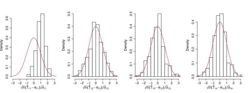
Figure 1: Histograms for $\sqrt{n}(\hat{T}_{ij}-\Theta^{*}_{ij})/\hat{\sigma}_{ij}$, $(i,j)\in\{(1,1),(1,2),(1,3),(1,4)\}$. The sample size was $n=500$ and the number of parameters $p=100$. The de-sparsified graphical Lasso estimator was calculated $300$ times. The model was the chain graph with $\rho=0.3$.

By Theorem 1, it follows that the $(1-\alpha)100\%$ asymptotic confidence interval for $\Theta^{*}_{ij}$ is given by

$$I_{ij}\equiv I_{ij}(\hat{\Theta}_{ij},\alpha,n):=[\hat{T}_{ij}-\Phi^{-1}(1-\alpha/2)\frac{\sigma_{ij}}{\sqrt{n}},\hat{T}_{ij}+\Phi^{-1}(1-\alpha/2)\frac{\sigma_{ij}}{\sqrt{n}}],$$

where we replace the unknown variance $\sigma_{ij}^{2}$ by the plug-in estimate $\hat{\sigma}_{ij}^{2}=\hat{\Theta}_{ii}\hat{\Theta}_{jj}+\hat{\Theta}_{ij}^{2}$ (Lemma 2). For each parameter $\Theta^{*}_{ij}$, the probability that the true value $\Theta^{*}_{ij}$ is covered by the confidence interval was estimated by its empirical version, $\hat{\alpha}_{ij}:=\mathbb{P}_{N}\mathbf{1}_{\{\Theta_{ij}^{*}\in I_{ij,\alpha}\}}.$ The number of iterations used to calculate the estimates $\hat{\alpha}_{ij}$ was set to $N=50.$ Next for a set $A\subset\mathcal{V}\times\mathcal{V}$ define the average coverage over the set $A$ as

$$\text{Avgcov}_{A}:=\frac{1}{|A|}\sum_{(i,j)\in A}\hat{\alpha}_{ij}.$$

After obtaining the estimates $\hat{\alpha}_{ij}$, we have averaged them over the sets $S$ and $S^{c}$ to obtain $Avgcov_{S}$ and $Avgcov_{S^{c}},$ respectively. Similarly, we have calculated the average length of the confidence interval for each parameter $\Theta^{*}_{ij}$ from $N=50$ iterations and again averaged these over the sets $S$ and $S^{c}$ to obtain $Avglength_{S}$ and $Avglength_{S^{c}}$.

We compare the performance of the graphical Lasso-based confidence intervals with three other methods. The first method is based on the oracle maximum likelihood estimator with the non-zero set $S$ pre-specified. This method only serves as a theoretical benchmark as it is asymptotically efficient if the true non-zero set $S$ is known. The second method is a post-model selection method: the maximum likelihood estimator is applied to the model selected by the graphical Lasso (see Lemma 9: under the irrepresentability condition, the graphical Lasso selects a model $\hat{S}\subseteq S$). Then the confidence intervals are constructed using asymptotic normality of the maximum likelihood estimator. The third method is based on the sample covariance matrix $\hat{\Sigma}$ which is the MLE estimator for $\Sigma^{*}$. Its inverse is then the maximum likelihood estimator for the precision matrix $\Theta^{*}$. In the fixed $p$ setting, the inverse sample covariance matrix $\hat{\Sigma}^{-1}$ is thus an asymptotically normal and efficient estimator of the precision matrix when the observations are Gaussian. This allows for construction of confidence intervals in the classical way, using asymptotic normality of $\hat{\Theta}=\hat{\Sigma}^{-1}$, hence the confidence interval for $\Theta^{*}_{ij}$ is given by $\hat{\Theta}_{ij}\pm\Phi^{-1}(1-\alpha/2)\frac{\hat{\sigma}_{ij}}{\sqrt{n}}$.

Table 1: The tables above show a comparison of four methods for construction of confidence intervals: the de-sparsified graphical Lasso (“De-sp. graphical Lasso”), the maximum likelihood estimator with specified set $S$ (“MLE with specified $S$”), the maximum likelihood estimator based on the non-zero set $\hat{S}$ selected by the graphical Lasso (“MLE based on $\hat{S}$”) and an estimator based on the sample covariance matrix $\hat{\Sigma}$ (“Sample covariance”). The table shows average coverages and average lengths of the constructed confidence intervals over the sets $S$ and $S^{c}$ (where applicable). For the method “MLE based on $\hat{S}$”, the reported averages are over $\hat{S}\cap S.$ The regularization parameter for the graphical Lasso was chosen $\lambda=\sqrt{\frac{\log p}{n}}$ in all simulations. The true precision matrix corresponds to a chain graph with $p$ vertices and $\rho$ equal to $0.3,0.4,0.2$ for settings S1,S2,S3, respectively

Estimated coverage probabilities and lengths

S1. $p=80,n=250,\rho=0.3$	$S$	$S$	$S^{c}$	$S^{c}$
	Avgcov	Avglength	Avgcov	Avglength
De-sp. graphical Lasso	0.934	0.247	0.972	0.215
MLE with specified $S$	0.940	0.308	–	–
MLE based on $\hat{S}$	0.887	0.325	–	–
Sample covariance	0.459	0.428	0.897	0.367

S2. $p=100,n=200,\rho=0.4$	$S$	$S$	$S^{c}$	$S^{c}$
	Avgcov	Avglength	Avgcov	Avglength
De-sp. graphical Lasso	0.925	0.288	0.974	0.250
MLE with specified $S$	0.945	0.349	–	–
MLE based on $\hat{S}$	0.856	0.374	–	–
Sample covariance	–	–	–	–

S3. $p=100,n=200,\rho=0.2$	$S$	$S$	$S^{c}$	$S^{c}$
	Avgcov	Avglength	Avgcov	Avglength
De-sp. graphical Lasso	0.951	0.301	0.964	0.263
MLE with specified $S$	0.943	0.357	–	–
MLE based on $\hat{S}$	0.747	0.328	–	–
Sample covariance	–	–	–	–

The results are reported in Tables 1 and 2. The de-sparsified graphical Lasso performs well also when compared to the oracle (“MLE with specified $S$”). In Table 1, settings S2 and S3 differ only in the value of $\rho.$ The de-sparsified graphical Lasso performs well for both of these settings, while the the post-model selection method (“MLE based on $\hat{S}$”) shows lower coverage for setting S3, where $\rho$ is comparable in magnitude to the noise level.

In table 2, the sample size is kept fixed at $n=100$ while the dimension of the parameter is increased, hence we observe lower coverage on $S$ for large values of $p$, as expected.

The choice of the regularization parameter Theory implies that the correct choice of the regularization parameter satisfies $\lambda_{n}\asymp\sqrt{\frac{\log p}{n}}$. Lemma 1 gives an explicit prescription for $\lambda$, however, this theoretically obtained value of $\lambda$ is very large. For all the numerical experiments, we have chosen $\lambda_{n}=\sqrt{\frac{\log p}{n}}$.

3.2 Real data experiment

We consider a dataset about riboflavin (vitamin $B_{2}$) production by bacillus subtilis without the response variable. The dataset is available from the R package hdi.

The dataset contains observations of $p=4088$ logarithms of gene expression levels from $n=71$ genetically engineered mutants of bacillus subtilis. We are interested in modeling the conditional independence structure of the covariates (logarithms of gene expression levels) and we try to estimate the associated graphical model using the de-sparsified graphical Lasso. We only consider the first $500$ covariates which have the highest variances.

In the first step, we split the sample and use 10 randomly chosen observations to estimate the variances of the $500$ variables. With the estimated variances, we scale the design matrix containing the remaining $61$ observations.

We calculate the graphical Lasso using the tuning parameter as in thesimulations, $\lambda=\sqrt{\log p/n}$, and hence calculate the de-sparsified graphical Lasso.

We threshold the de-sparsified graphical Lasso at level $\Phi^{-1}(1-\frac{\alpha}{p(p-1)})\hat{\sigma}_{ij}/\sqrt{n},$ where $\alpha=0.05$ and $\hat{\sigma}_{ij}^{2}=\hat{\Theta}_{ii}\hat{\Theta}_{ii}+\hat{\Theta}_{ij}^{2}$ is an estimate of the asymptotic variance calculated under the assumption of normality and using the graphical Lasso estimator $\hat{\Theta}.$ We identify $5$ edges as significant.

For independently permuted variables (for each variable, a different permutation is used), the conditional dependencies are broken (the truth isthe empty graph), and the de-sparsified graphical Lasso correctly detects zero edges.

Table 2: A table showing the performance of the de-sparsified graphical Lasso for number of parameters $p$ taking values $100,200,300,500$ and $n=100$. The regularization parameter was chosen $\lambda=\sqrt{\frac{\log p}{n}}$ in all simulations. The constant $\rho$ is $0.3$ in the definition of $\Theta^{*}$

Estimated coverage probabilities and lengths

Chain graph	$S$	$S$	$S^{c}$	$S^{c}$
	Avgcov	Avglength	Avgcov	Avglength
p = 100	0.931	0.401	0.978	0.348
p = 200	0.917	0.400	0.984	0.349
p = 300	0.893	0.401	0.988	0.349
p = 500	0.832	0.401	0.988	0.350

4 Proofs

Lemma 3.

Suppose that $X_{1},\dots,X_{n}\in\mathbb{R}^{p}$ are independent and distributed as $X=(X^{1},\dots,X^{p})$ with $\mathbb{E}X=0,$ $\text{cov}(X)=\Sigma^{*}.$ Let $\Theta^{*}=(\Sigma^{*})^{-1}$ exist and satisfy the irrepresentability condition (A1) with a constant $\alpha\in(0,1]$. Let $\hat{\Theta}_{n}$ be the solution to the optimization problem (P1) with tuning parameter $\lambda_{n}=\frac{8}{\alpha}\delta_{n}$ for some $\delta_{n}>0$ and suppose that the sparsity assumption

$$d\leq\frac{1}{6(1+8/\alpha)\max\{\kappa_{\Sigma^{*}}\kappa_{\Gamma^{*}},\kappa_{\Sigma^{*}}^{3}\kappa_{\Gamma^{*}}^{2}\}\delta_{n}}$$ (13)

is satisfied. Then on the set $\mathcal{T}_{n}=\{\|\hat{\Sigma}-\Sigma^{*}\|_{\infty}<\delta_{n}\},$ we have

Bound I

$$\|\emph{rem}\|_{\infty}=\mathcal{O}\biggl{(}\frac{1}{\alpha}\kappa_{\Gamma^{*}}\max\{{d}\delta_{n}\|\Theta^{*}W\|_{\infty},\frac{1}{\alpha}\kappa_{\Gamma^{*}}d^{2}\delta^{3}_{n},\frac{1}{\alpha}\kappa_{\Gamma^{*}}\kappa_{\Sigma^{*}}d\delta^{2}_{n}\}\biggr{)}$$ (14)

Bound II

$$\|\emph{rem}\|_{\infty}=\mathcal{O}\biggl{(}\frac{1}{\alpha}\kappa_{\Gamma^{*}}\max\{{d}\delta_{n}\|\Theta^{*}W\|_{\infty},\frac{1}{\alpha^{2}}\kappa_{\Gamma^{*}}d^{2}\delta^{3}_{n},\frac{1}{\alpha}\Lambda_{\max}(\Theta^{*}){d}^{3/2}\delta^{2}_{n}\}\biggr{)}.$$ (15)

Proof of Lemma 3.

The KKT conditions for the optimization problem (P1) read

$$\hat{\Sigma}-\hat{\Theta}^{-1}+\lambda\hat{Z}=0,$$ (16)

where the matrix $\hat{Z}$ is the sub-differential of $\|.\|_{1,\text{off}}$ at the optimum $\hat{\Theta}$. Multiplying (16) by $\hat{\Theta}$ from both sides (which is equivalent to multiplying the vectorized equation (16) by $\hat{\Theta}\otimes\hat{\Theta}$), we obtain

$$\hat{\Theta}\hat{\Sigma}\hat{\Theta}-\hat{\Theta}+\hat{\Theta}\lambda\hat{Z}\hat{\Theta}=0.$$

Adding $\hat{\Theta}-\Theta^{*}$ to both sides and rearranging gives

$$\underbrace{\hat{\Theta}+\hat{\Theta}\lambda\hat{Z}\hat{\Theta}}_{\hat{T}}-\Theta^{*}=-\Theta^{*}(\hat{\Sigma}-\Sigma^{*})\Theta^{*}+\text{rem},$$ (17)

where, denoting $W:=\hat{\Sigma}-\Sigma^{*}$, we have

$$\text{rem}:=-(\hat{\Theta}-\Theta^{*})W\Theta^{*}-(\hat{\Theta}\hat{\Sigma}-I)(\hat{\Theta}-\Theta^{*}).$$ (18)

Bound I

$$\|\text{rem}\|_{\infty} \leq \|(\hat{\Theta}-\Theta^{*})W\Theta^{*}\|_{\infty}+\|(\hat{\Theta}\hat{\Sigma}-I)(\hat{\Theta}-\Theta^{*})\|_{\infty}$$

$$\leq {\left|\kern-1.07639pt\left|\kern-1.07639pt\left|\hat{\Theta}-\Theta^{*}\right|\kern-1.07639pt\right|\kern-1.07639pt\right|}_{\infty}\|W\Theta^{*}\|_{\infty}+\|\hat{\Theta}\hat{\Sigma}-I\|_{\infty}{\left|\kern-1.07639pt\left|\kern-1.07639pt\left|\hat{\Theta}-\Theta^{*}\right|\kern-1.07639pt\right|\kern-1.07639pt\right|}_{\infty}$$

We can bound

$$\|\hat{\Sigma}\hat{\Theta}-I\|_{\infty} = \|(\hat{\Sigma}-\Sigma^{*})(\hat{\Theta}-\Theta^{*})+\Sigma^{*}(\hat{\Theta}-\Theta^{*})+(\hat{\Sigma}-\Sigma^{*})\Theta^{*}\|_{\infty}$$

$$\leq \|\hat{\Sigma}-\Sigma^{*}\|_{\infty}{\left|\kern-1.07639pt\left|\kern-1.07639pt\left|\hat{\Theta}-\Theta^{*}\right|\kern-1.07639pt\right|\kern-1.07639pt\right|}_{\infty}+{\left|\kern-1.07639pt\left|\kern-1.07639pt\left|\Sigma^{*}\right|\kern-1.07639pt\right|\kern-1.07639pt\right|}_{\infty}\|\hat{\Theta}-\Theta^{*}\|_{\infty}+\|W\Theta^{*}\|_{\infty}$$

Hence

$$\|\text{rem}\|_{\infty} \leq \underbrace{{\left|\kern-1.07639pt\left|\kern-1.07639pt\left|\hat{\Theta}-\Theta^{*}\right|\kern-1.07639pt\right|\kern-1.07639pt\right|}_{\infty}\|W\Theta^{*}\|_{\infty}}_{\text{rem}_{1}}+\underbrace{\|\hat{\Sigma}-\Sigma^{*}\|_{\infty}{\left|\kern-1.07639pt\left|\kern-1.07639pt\left|\hat{\Theta}-\Theta^{*}\right|\kern-1.07639pt\right|\kern-1.07639pt\right|}^{2}_{\infty}}_{\text{rem}_{2}}$$

$$+\underbrace{{\left|\kern-1.07639pt\left|\kern-1.07639pt\left|\Sigma^{*}\right|\kern-1.07639pt\right|\kern-1.07639pt\right|}_{\infty}\|\hat{\Theta}-\Theta^{*}\|_{\infty}{\left|\kern-1.07639pt\left|\kern-1.07639pt\left|\hat{\Theta}-\Theta^{*}\right|\kern-1.07639pt\right|\kern-1.07639pt\right|}_{\infty}}_{\text{rem}_{3}}+\underbrace{\|W\Theta^{*}\|_{\infty}{\left|\kern-1.07639pt\left|\kern-1.07639pt\left|\hat{\Theta}-\Theta^{*}\right|\kern-1.07639pt\right|\kern-1.07639pt\right|}_{\infty}}_{\text{rem}_{1}}$$

In what follows, condition on the event $\mathcal{T}_{n}=\{\|\hat{\Sigma}-\Sigma^{*}\|_{\infty}\leq\delta_{n}\}$. Note that ${\left|\kern-1.07639pt\left|\kern-1.07639pt\left|\Theta^{*}\right|\kern-1.07639pt\right|\kern-1.07639pt\right|}_{\infty}=\max_{i}\|\Theta_{i}\|_{1}\leq\max_{i}\|\Theta_{i}\|_{2}\sqrt{d}\leq\Lambda_{\max}(\Theta^{*})\sqrt{d}$.

By Lemma 9, part (a), on $\mathcal{T}$ it holds that $\hat{\Theta}_{S^{c}}=\Theta^{*}_{S^{c}}$. Thus $\hat{\Theta}$ has at most $d$ nonzero entries per row. Hence it follows

$${\left|\kern-1.07639pt\left|\kern-1.07639pt\left|\Delta\right|\kern-1.07639pt\right|\kern-1.07639pt\right|}_{\infty}={\left|\kern-1.07639pt\left|\kern-1.07639pt\left|\hat{\Theta}-\Theta^{*}\right|\kern-1.07639pt\right|\kern-1.07639pt\right|}_{\infty}\leq d\|\hat{\Theta}-\Theta^{*}\|_{\infty}.$$ (19)

Next by Lemma 9, part (b), we have the bound

$$\|\hat{\Theta}-\Theta^{*}\|_{\infty}\leq 2(1+8/\alpha)\kappa_{\Gamma^{*}}\delta_{n}.$$

We obtain

$$\|\text{rem}_{1}\|_{\infty} \leq \|\Theta^{*}W\|_{\infty}{\left|\kern-1.07639pt\left|\kern-1.07639pt\left|\Delta\right|\kern-1.07639pt\right|\kern-1.07639pt\right|}_{1}\leq 2(1+8/\alpha)\kappa_{\Gamma^{*}}{d}\delta_{n}\|\Theta^{*}W\|_{\infty}$$

$$\|\text{rem}_{2}\|_{\infty} \leq {\left|\kern-1.07639pt\left|\kern-1.07639pt\left|\Delta\right|\kern-1.07639pt\right|\kern-1.07639pt\right|}_{1}^{2}\|W\|_{\infty}\leq 4(1+8/\alpha)^{2}\kappa_{\Gamma^{*}}^{2}d^{2}\delta^{3}_{n}$$

$$\|\text{rem}_{3}\|_{\infty} \leq \|\Delta\|_{\infty}{\left|\kern-1.07639pt\left|\kern-1.07639pt\left|\Delta\right|\kern-1.07639pt\right|\kern-1.07639pt\right|}_{1}{\left|\kern-1.07639pt\left|\kern-1.07639pt\left|\Sigma^{*}\right|\kern-1.07639pt\right|\kern-1.07639pt\right|}_{1}\leq 4(1+8/\alpha)^{2}\kappa_{\Gamma^{*}}^{2}\kappa_{\Sigma^{*}}d\delta^{2}_{n}.$$

Hence conditioned on $\mathcal{T},$

$$\|\text{rem}\|_{\infty} \leq 4\max\{2(1+8/\alpha)\kappa_{\Gamma^{*}}{d}\delta_{n}\|\Theta^{*}W\|_{\infty},$$

$$4(1+8/\alpha)^{2}\kappa_{\Gamma^{*}}^{2}d^{2}\delta^{3}_{n},$$

$$4(1+8/\alpha)^{2}\kappa_{\Gamma^{*}}^{2}\kappa_{\Sigma^{*}}d\delta^{2}_{n}\}$$

$$= \mathcal{O}\left(\frac{1}{\alpha}\kappa_{\Gamma^{*}}\max\{{d}\delta_{n}\|\Theta^{*}W\|_{\infty},\frac{1}{\alpha}\kappa_{\Gamma^{*}}d^{2}\delta^{3}_{n},\frac{1}{\alpha}\kappa_{\Gamma^{*}}\kappa_{\Sigma^{*}}d\delta^{2}_{n}\}\right).$$

Bound II
Observe that

$${\left|\kern-1.07639pt\left|\kern-1.07639pt\left|\hat{\Theta}\right|\kern-1.07639pt\right|\kern-1.07639pt\right|}_{1}\leq{\left|\kern-1.07639pt\left|\kern-1.07639pt\left|\hat{\Theta}-\Theta^{*}\right|\kern-1.07639pt\right|\kern-1.07639pt\right|}_{1}+{\left|\kern-1.07639pt\left|\kern-1.07639pt\left|\Theta^{*}\right|\kern-1.07639pt\right|\kern-1.07639pt\right|}_{1}\leq 2(1+8/\alpha)\kappa_{\Gamma^{*}}d\delta_{n}+\sqrt{d}\Lambda_{\max}(\Theta^{*}).$$

By (18) and using the KKT conditions we have

$$\hskip 1.0pt\|\text{rem}\|_{\infty}={} \|\Delta W\Theta^{*}-\hat{\Theta}(\hat{\Sigma}-\hat{\Theta}^{-1})\|_{\infty}$$

$$\leq{} \|\Delta W\Theta^{*}\|_{\infty}+{\left|\kern-1.07639pt\left|\kern-1.07639pt\left|\hat{\Theta}\right|\kern-1.07639pt\right|\kern-1.07639pt\right|}_{1}\|\lambda\hat{Z}\|_{\infty}\|\Delta\|_{\infty}$$

$$\leq{} 2(1+8/\alpha)\kappa_{\Gamma^{*}}{d}\delta_{n}\|\Theta^{*}W\|_{\infty}$$

$${}+16\frac{8}{\alpha}4(1+8/\alpha)^{2}\kappa_{\Gamma^{*}}^{2}d^{2}\delta^{3}_{n}+2\frac{8}{\alpha}(1+8/\alpha)\Lambda_{\max}(\Theta^{*})\kappa_{\Gamma^{*}}{d}^{3/2}\delta^{2}_{n}$$

$$={} \mathcal{O}\left(\frac{1}{\alpha}\kappa_{\Gamma^{*}}\max\{{d}\delta_{n}\|\Theta^{*}W\|_{\infty},\frac{1}{\alpha^{2}}\kappa_{\Gamma^{*}}d^{2}\delta^{3}_{n},\frac{1}{\alpha}\Lambda_{\max}(\Theta^{*}){d}^{3/2}\delta^{2}_{n}\}\right).\qed\hskip 1.0pt$$

Proof of Lemma 1.

(i) Under (C1), using Lemma 8 and by assumption (A2) we have

$$\|\Theta^{*}W\|_{\infty} \leq {\left|\kern-1.07639pt\left|\kern-1.07639pt\left|\Theta^{*}\right|\kern-1.07639pt\right|\kern-1.07639pt\right|}_{\infty}\|W\|_{\infty}=\max_{i=1,\dots,p}\|\Theta^{*}_{i}\|_{1}\|W\|_{\infty}$$

$$\leq \sqrt{d}\|\Theta_{i}^{*}\|_{2}\|W\|_{\infty}=\mathcal{O}_{\mathbb{P}}(\sqrt{d\log p/n}).$$

Then by Lemma 3, bound II,

$$\|\text{rem}\|_{\infty} = \mathcal{O}_{\mathbb{P}}\left(\frac{1}{\alpha}\kappa_{\Gamma^{*}}\max\{{d}\delta_{n}\|\Theta^{*}W\|_{\infty},\frac{1}{\alpha^{2}}\kappa_{\Gamma^{*}}d^{2}\delta^{3}_{n},\frac{1}{\alpha}\Lambda_{\max}(\Theta^{*}){d}^{3/2}\delta^{2}_{n}\}\right)$$

$$= \mathcal{O}_{\mathbb{P}}\left(\frac{1}{\alpha^{2}}\kappa_{\Gamma^{*}}\max\{{d}^{3/2}\log p/n,\frac{1}{\alpha}\kappa_{\Gamma^{*}}d^{2}(\log p/n)^{3/2}\}\right).$$

(ii) Under (C2) and (A2), by Lemma 7 we have

$$\|\Theta^{*}W\|_{\infty}=\max_{i,j=1,\dots,p}|\Theta^{*}_{i}We_{j}|=\mathcal{O}_{\mathbb{P}}(\sqrt{\log p/n}).$$

Hence using Lemma 3, bound I and Lemma 8 we have

$$\|\text{rem}\|_{\infty} =\mathcal{O}_{\mathbb{P}}\left(\frac{1}{\alpha}\kappa_{\Gamma^{*}}\max\{{d}\log p/n,\frac{1}{\alpha}\kappa_{\Gamma^{*}}d^{2}(\log p/n)^{3/2},\frac{\kappa_{\Gamma^{*}}\kappa_{\Sigma^{*}}}{\alpha}d\log p/n\}\right)$$

$$\stackrel{{\scriptstyle(a)}}{{=}}\mathcal{O}_{\mathbb{P}}\left(\frac{1}{\alpha^{2}}\kappa^{2}_{\Gamma^{*}}\kappa_{\Sigma^{*}}d\log p/n\right).$$

Step (a) above follows by the sparsity assumption (13) and since $\kappa_{\Gamma^{*}}\gtrsim 1$. The latter statement follows by (A2), using that $\Lambda_{\min}((\Gamma^{*}_{SS})^{-1})=1/\Lambda_{\max}(\Gamma^{*}_{SS})\geq 1/\Lambda_{\max}(\Gamma^{*})$ and that the eigenvalues of Kronecker product satisfy $\Lambda_{\max}(\Sigma\otimes\Sigma)=\Lambda^{2}_{\max}(\Sigma)$. ∎

Proof of Theorem 1.

By Lemma 1, under the sub-Gaussianity condition (C1) or (C2), under the appropriate sparsity assumptions (combining (13) and (14), (15)) it holds that $\|\text{rem}\|_{\infty}=o_{\mathbb{P}}(1).$ Hence for every $(i,j)$ it holds that

$$\sqrt{n}(\hat{T}_{ij}-\Theta^{*}_{ij})=\frac{1}{\sqrt{n}}\sum_{k=1}^{n}({\Theta^{*}_{i}}^{T}X_{k}{\Theta^{*}_{j}}^{T}X_{k}-\Theta^{*}_{ij})+o_{\mathbb{P}}(1).$$ (20)

It remains to prove that the scaled summation term in (20) weakly converges to the normal distribution. To this end, define

$$Z_{ij,k}:={\Theta^{*}_{i}}^{T}X_{k}{\Theta^{*}_{j}}^{T}X_{k}-\Theta^{*}_{ij}.$$

For each $n$ fixed, $Z_{ij,1},\dots,Z_{ij,n}$ are identically distributed r.v.s with mean $\mathbb{E}(Z_{ij,k})=(\Theta^{*}_{i})^{T}\Sigma^{*}\Theta^{*}_{j}-\Theta_{ij}=e_{i}^{T}\Theta^{*}\Sigma^{*}\Theta^{*}e_{j}-\Theta^{*}_{ij}=0$.

Since each $X_{k}$ has sub-Gaussian elements, the variance $\sigma_{ij}^{2}=\text{Var}(Z_{ij,k})=\text{Var}({\Theta^{*}_{i}}^{T}X_{k}{\Theta^{*}_{j}}^{T}X_{k})$ is finite. Denote $S_{n}=\sum_{k=1}^{n}Z_{ij,k}$. Then $s_{n}:=\text{var}(S_{n})=n\sigma^{2}_{ij}.$ Dividing (20) by $\sigma_{ij}>0,$ we obtain

$$\sqrt{n}{(\hat{T}_{ij}-\Theta^{*}_{ij})}/{\sigma_{ij}}=S_{n}/s_{n}+{o_{\mathbb{P}}(1)}/{\sigma_{ij}}.$$

First note that by the assumption $1/\sigma_{ij}=\mathcal{O}(1)$ we have $o_{\mathbb{P}}(1)/\sigma_{ij}=o_{\mathbb{P}}(1).$

(i) Sub-Gaussian design (C1)

To show $S_{n}/s_{n}\rightsquigarrow\mathcal{N}(0,1)$, we check the Lindeberg condition, i.e. for all $\varepsilon>0$

$$\lim_{n\rightarrow\infty}\frac{1}{s_{n}^{2}}\sum_{k=1}^{n}\mathbb{E}(Z_{ij,k}^{2}\mathbf{1}(|Z_{ij,k}|>\varepsilon s_{n}))=0.$$

Observe that since $\{Z_{ij,k}\}_{k=1}^{n}$ are identically distributed for $n$ fixed and $s_{n}^{2}=n\sigma_{ij}^{2}$,

$$\sum_{k=1}^{n}\frac{1}{s_{n}^{2}}\mathbb{E}(Z_{ij,k}^{2}\mathbf{1}(|Z_{ij,k}|>\varepsilon s_{n}))=\frac{1}{\sigma_{ij}^{2}}\mathbb{E}(Z_{ij,1}^{2}\mathbf{1}(|Z_{ij,1}|>\varepsilon s_{n})).$$

Consequently, it remains to show that $\lim_{n\rightarrow\infty}\mathbb{E}(Z_{ij,1}^{2}\mathbf{1}(|Z_{ij,1}|>\varepsilon s_{n}))=0.$ For any $c>0$ we may rewrite

$$c=\int_{0}^{\infty}\mathbf{1}_{c>t}dt.$$

Therefore, applying the last observation and by Fubini’s theorem we obtain

$$\int_{\Omega}|X|^{2}\mathbf{1}_{|X|>a}d\mathbb{P}=a^{2}\mathbb{P}(|X|>a)+2\int_{a}^{\infty}u\mathbb{P}(|X|>u)du.$$

Then it follows

$$\mathbb{E}(Z_{ij,1}^{2}\mathbf{1}(|Z_{ij,1}|>\varepsilon\sigma_{ij}\sqrt{n})) \leq \varepsilon^{2}\sigma_{ij}^{2}{n}\mathbb{P}(|Z_{ij,1}|>\varepsilon\sigma_{ij}\sqrt{n})$$

$$+\int_{\varepsilon\sigma_{ij}\sqrt{n}}^{\infty}x\mathbb{P}(|Z_{ij,1}|>x)dx.$$

To show that the limit of the right-hand side of the last inequality is $0$ for $n\rightarrow\infty$, we use Lemma 4, by which it follows that $Z_{ij,1}$ satisfies a tail bound $\mathbb{P}(|Z_{ij,1}|>t)\leq 4de^{-\frac{t}{c_{1}d}}$. For a fixed $\varepsilon>0,$ putting $t:=\varepsilon\sigma_{ij}\sqrt{n},$ we obtain

$$\mathbb{P}(|Z_{ij,1}|>\varepsilon\sigma_{ij}\sqrt{n})\leq 4de^{-\frac{\varepsilon\sigma_{ij}\sqrt{n}}{c_{1}d}}.$$

Consequently, for the first term in (4) we have

$$\lim_{n\rightarrow\infty}\sigma_{ij}^{2}{n}P(|Z_{ij,1}|>\varepsilon\sigma_{ij}\sqrt{n})\leq\lim_{n\rightarrow\infty}\sigma_{ij}^{2}{n}de^{-\frac{\varepsilon\sigma_{ij}\sqrt{n}}{c_{1}d}}=0,$$ (21)

which follows by the sparsity assumption (8) that implies $d^{\frac{3}{2}}=o({\sqrt{n}}/{\log p}).$ Next considering the limit of the last term in (4), we have

$$\int_{\varepsilon\sigma_{ij}\sqrt{n}}^{\infty}xP(|Z_{ij,1}|>x)dx\leq\int_{\varepsilon\sigma_{ij}\sqrt{n}}^{\infty}4xde^{-\frac{x}{c_{1}d}}dx.$$

In the integral, substitute $t:=\frac{x}{\sigma_{ij}\sqrt{n}}$ to obtain

$$\lim_{n\rightarrow\infty}\int_{\sigma_{ij}\sqrt{n}}^{\infty}dxe^{-\frac{x}{d}}dx=\lim_{n\rightarrow\infty}\int_{1}^{\infty}d\sigma_{ij}^{2}nte^{-\frac{\sigma_{ij}\sqrt{n}}{d}t}dt.$$

Again by the restriction on $d$ and the Lebesgue dominated convergence it then follows that the limit of the integral is $0$. In conclusion, we get ${S_{n}}/{s_{n}}\rightsquigarrow\mathcal{N}(0,1)$ for $n\rightarrow\infty$.

(ii) Sub-Gaussian design (C2)

Under (C2), we have a bound $\mathbb{P}(|Z_{ij,1}|>t)\lesssim e^{-t/(c_{2}K^{2})}$ hence similarly as in (i), asymptotic normality follows. ∎

Lemma 4.

Let $\Theta^{*}$ satisfy assumption (A2) and let the random vector $X\in\mathbb{R}^{p}$ satisfy the sub-Gaussianity condition (C1) with $K=\mathcal{O}(1)$. Then for $t>c_{0}$ the random variable $Z:={\Theta^{*}_{i}}^{T}X{\Theta^{*}_{j}}^{T}X-\Theta^{*}_{ij}$ satisfies the following bound

$$\mathbb{P}(|Z|>t)\leq 4de^{{-\frac{t}{c_{1}d}}},$$

where $c_{0},c_{1}$ do not depend on $n.$

Proof.

Since $|{\Theta^{*}_{i}}^{T}X|\leq\|\Theta_{i}\|_{1}\max_{k:\Theta^{*}_{ki}\not=0}|{X^{k}}|\leq\|\Theta^{*}_{i}\|_{2}\sqrt{d}\max_{k:\Theta^{*}_{ki}\not=0}|{X^{k}}|,$ and using the union bound and sub-Gaussianity of $X_{n}^{k}/\sqrt{\Sigma_{kk}^{*}}$ by assumption (C1) gives

$$\mathbb{P}(|{\Theta^{*}_{i}}^{T}X|>t) \leq \mathbb{P}\left(\max_{k:\Theta^{*}_{ki}\not=0}|X^{k}|>\frac{{t}}{\sqrt{d}\|\Theta^{*}_{i}\|_{2}}\right)$$

$$\leq d\max_{k:\Theta^{*}_{ki}\not=0}\mathbb{P}\left(|X^{k}|/\sqrt{\Sigma_{kk}^{*}}>\frac{{t}}{\sqrt{d}\|\Theta^{*}_{i}\|_{2}\sqrt{\Sigma_{kk}^{*}}}\right)$$

$$\leq 2d\exp\left({-\frac{{t^{2}}}{6K^{2}d\|\Theta^{*}_{i}\|^{2}_{2}\max_{k}{\Sigma_{kk}^{*}}}}\right).$$

Then for ${\Theta^{*}_{i}}^{T}X{\Theta^{*}_{j}}^{T}X$ we obtain the bound

$$\mathbb{P}(|{\Theta^{*}_{i}}^{T}X{\Theta^{*}_{j}}^{T}X|>t)\leq 4d\exp\left({-\frac{{t}}{6K^{2}d\Lambda^{2}_{\max}(\Theta^{*})\max_{k}{\Sigma_{kk}^{*}}}}\right).$$

Under (A2), $\Sigma^{*}_{kk}$ and $\|\Theta^{*}_{i}\|_{2}\leq\Lambda_{\max}(\Theta^{*})$ are uniformly bounded in $n$. Thus for $Z={\Theta^{*}_{i}}^{T}X{\Theta^{*}_{j}}^{T}X-\Theta^{*}_{ij},$ there exist constants $c_{0},c_{1},c_{2}$ not depending on $n$ such that for $t>c_{0}>|\Theta^{*}_{ij}|$

$$\mathbb{P}(|Z|>t)\leq 4de^{{-\frac{t-|\Theta^{*}_{ij}|}{c_{2}d}}}\leq 4de^{{-\frac{t}{c_{1}d}}},$$

since ${|\Theta^{*}_{ij}|}/{d}$ is bounded by (A2) and $d\geq 1$. ∎

Proof of Lemma 2.

Since $X\sim\mathcal{N}(0,\Sigma^{*}),$ then ${\Theta^{*}}X\sim\mathcal{N}(0,\Theta^{*}),$ hence

$$\sigma_{ij}^{2}=\text{Var}({\Theta^{*}_{i}}^{T}X{\Theta^{*}_{j}}^{T}X)=\text{Var}(e_{i}^{T}{\Theta^{*}}^{T}XX^{T}{\Theta^{*}}e_{j})=\text{Var}(e_{i}^{T}ZZ^{T}e_{j}),$$

where $Z\sim\mathcal{N}(0,\Theta^{*}).$ Thus

$$\sigma_{ij}^{2} = \text{Var}(Z^{i}Z^{j})=\mathbb{E}((Z^{i})^{2}(Z^{j})^{2})-\mathbb{E}(Z^{i}Z^{j})^{2}$$

$$= \Theta^{*}_{ii}\Theta^{*}_{jj}+2{\Theta^{*}_{ij}}^{2}-{\Theta^{*}_{ij}}^{2}=\Theta^{*}_{ii}\Theta^{*}_{jj}+{\Theta^{*}_{ij}}^{2}.$$

By assumption (A2), ${\Theta^{*}_{ii}\Theta^{*}_{jj}+{\Theta^{*}}_{ij}^{2}}\geq\Lambda^{2}_{\min}(\Theta^{*})\geq\frac{1}{L^{2}}>0$, where $L\asymp 1$, therefore $1/\sigma_{ij}=\mathcal{O}(1)$.

By Lemma 9 and Lemma 8 we have

$$|\hat{\sigma}_{ij}^{2}-\sigma_{ij}^{2}| \leq |\hat{\Theta}_{ii}\hat{\Theta}_{jj}-\Theta^{*}_{ii}\Theta^{*}_{jj}|+|\hat{\Theta}_{ij}^{2}-{\Theta^{*}}_{ij}^{2}|$$ (22)

$$\leq |\Delta_{ii}\Delta_{jj}+\Theta^{*}_{ii}\Delta_{jj}+\Theta^{*}_{jj}\Delta_{ii}|$$

$$\;+\;\;|\Delta_{ij}(\Delta_{ij}+2\Theta^{*}_{ij})|$$

$$= \mathcal{O}_{\mathbb{P}}\left(1/\alpha\kappa_{\Gamma^{*}}\sqrt{\frac{\log p}{n}}\right),$$

where we used assumption (A2) and the sparsity assumption (13). ∎

Concentration for sub-Gaussian design (C2)

Lemma 5.

Let $\alpha,\beta\in\mathbb{R}^{p}$ such that $\|\alpha\|_{2}\leq M,\|\beta\|_{2}\leq M.$ Let $X_{k}\in\mathbb{R}^{p}$ satisfy the sub-Gaussianity assumption (C2) with a constant $K>0.$ Then for $m\geq 2,$

$$\mathbb{E}|\alpha^{T}X_{k}X_{k}^{T}\beta-\mathbb{E}\alpha^{T}X_{k}X_{k}^{T}\beta|^{m}/(2M^{2}K^{2})^{m}\leq\frac{m!}{2}.$$

Consequently, we may apply Bernstein inequality (Lemma 14.9 in [Bühlmann and van de Geer [2011]]).

Lemma 6.

Let $\alpha,\beta\in\mathbb{R}^{p}$ such that $\|\alpha\|_{2}\leq M,\|\beta\|_{2}\leq M.$ Let $X_{k}\in\mathbb{R}^{p}$ satisfy the sub-Gaussianity assumption (C2) with a constant $K>0.$ For all $t>0$

$$\mathbb{P}\left(|\alpha^{T}\hat{\Sigma}\beta-\alpha^{T}\Sigma\beta|/(2M^{2}K^{2})>t+\sqrt{2t}\right)\leq 2e^{-nt}.$$

Lemma 7.

Assume $\|\alpha_{i}\|_{2}\leq M,\|\beta\|_{2}\leq M$ for all $i=1,\dots,p$ and (C2) with $K$. For all $t>0$ it holds

$$\mathbb{P}\Biggl{(}\max_{i=1,\dots,p}|\alpha_{i}^{T}(\hat{\Sigma}-\Sigma)\beta|/(2M^{2}K^{2})>t+\sqrt{2t}+\sqrt{\frac{2\log(2p)}{n}}+\frac{\log(2p)}{n}\Biggr{)}\leq e^{-nt}.$$

Proof.

By Lemma 5 we have

$$\mathbb{E}|\alpha^{T}X_{k}X_{k}^{T}\beta-\mathbb{E}\alpha^{T}X_{k}X_{k}^{T}\beta|^{m}/(2M^{2}K^{2})^{m}\leq\frac{m!}{2}.$$

Lemma 14.13 in [Bühlmann and van de Geer [2011]] gives the claim. ∎

Proof of Lemma 5.

By assumption we have $\|\alpha\|_{2}\leq M,\|\beta\|_{2}\leq M.$ Consequently, by the sub-Gaussianity assumption with a constant $K$ we obtain

$$\mathbb{E}e^{|X_{k}^{T}\alpha|^{2}/(MK)^{2}}\leq 2$$

and likewise

$$\mathbb{E}e^{|X_{k}^{T}\beta|^{2}/(MK)^{2}}\leq 2.$$

Next by the inequality $ab\leq a^{2}/2+b^{2}/2$ (for any $a,b\in\mathbb{R}$) and by the Cauchy-Schwarz inequality we obtain

$$\mathbb{E}e^{|\alpha^{T}X_{k}X_{k}^{T}\beta|/(MK)^{2}} \leq \mathbb{E}e^{|X_{k}^{T}\alpha|^{2}/(MK)^{2}/2}e^{|X_{k}^{T}\beta|^{2}/(MK)^{2}/2}$$

$$\leq \{\mathbb{E}e^{|X_{k}^{T}\alpha|^{2}/(MK)^{2}}\}^{1/2}\{\mathbb{E}e^{|X_{k}^{T}\beta|^{2}/(MK)^{2}}\}^{1/2}$$

$$\leq 2.$$

By the Taylor expansion, we have the inequality

$$1+\frac{1}{m!}\mathbb{E}|\alpha^{T}X_{k}X_{k}^{T}\beta|^{m}/(MK)^{2m}\leq\mathbb{E}e^{|\alpha^{T}X_{k}X_{k}^{T}\beta|/(MK)^{2}}$$

Next it follows

$$\mathbb{E}|\alpha^{T}X_{k}X_{k}^{T}\beta-\mathbb{E}\alpha^{T}X_{k}X_{k}^{T}\beta|^{m}/(MK)^{2m} \leq 2^{m-1}\mathbb{E}|\alpha^{T}X_{k}X_{k}^{T}\beta|^{m}/(MK)^{2m}$$

$$\leq 2^{m-1}m!(\mathbb{E}e^{|\alpha^{T}X_{k}X_{k}^{T}\beta|/(MK)^{2}}-1)$$

$$=2^{m-1}m!=\frac{m!}{2}2^{m}.$$

And thus

$$\mathbb{E}|\alpha^{T}X_{k}X_{k}^{T}\beta-\mathbb{E}\alpha^{T}X_{k}X_{k}^{T}\beta|^{m}/(2M^{2}K^{2})^{m}\leq\frac{m!}{2}.\qed$$

Appendix A Tail bounds and rates of convergence

The following Lemma from [Ravikumar et al. [2008]] gives probabilistic bounds for the event $\mathcal{T}_{n}$ if $X$ satisfies (C1).

Lemma 8 ([Ravikumar et al. [2008]], sub-Gaussian model).

Let $X=(X^{1},\dots,X^{p})$ be independent, distributed as $X$ with $\mathbb{E}X=0,$ $\text{cov}(X)=\Sigma^{*}=(\Theta^{*})^{-1}$ and satisfying (C1) with $K>0$. Then for

$$\delta_{\tau}(n,r)=8(1+12K^{2})\max_{i}\Sigma^{*}_{ii}\sqrt{2\frac{\log(4r)}{n}},$$

and for every $\gamma>2$ and each $n$ such that $\delta_{\tau}(n,p^{\gamma})<8(1+12K^{2})\max_{i}\Sigma^{*}_{ii}$ we have

$$\mathbb{P}\left(\|\hat{\Sigma}-\Sigma^{*}\|_{\infty}\geq\delta_{\tau}(n,p^{\gamma})\right)\leq\frac{1}{p^{\gamma-2}}.$$

We restate a result on rates of convergence of the graphical Lasso from [Ravikumar et al. [2008]] in Lemma 9.

Lemma 9 (Theorem 1, [Ravikumar et al. [2008]]).

Suppose that $X_{1},\dots,X_{n}\in\mathbb{R}^{p}$ are independent and distributed as $X=(X^{1},\dots,X^{p})$ with $\mathbb{E}X=0,$ $\text{cov}(X)=\Sigma^{*}.$ Let $\Theta^{*}=(\Sigma^{*})^{-1}$ exist and satisfy the irrepresentability condition (A1) with a constant $\alpha\in(0,1]$. Denote $S^{c}$ to be the set of indices that correspond to zero entries of $\Theta^{*}.$ Let $\hat{\Theta}_{n}$ be the solution to the optimization problem (P1) with tuning parameter $\lambda_{n}=\frac{8}{\alpha}\delta_{n}$ for some $\delta_{n}>0$ and suppose that the sparsity assumption

$$d\leq\frac{1}{6(1+8/\alpha)\max\{\kappa_{\Sigma^{*}}\kappa_{\Gamma^{*}},\kappa_{\Sigma^{*}}^{3}\kappa_{\Gamma^{*}}^{2}\}\delta_{n}}$$

is satisfied. Then on $\mathcal{T}_{n}=\{\|\hat{\Sigma}-\Sigma\|_{\infty}\leq\delta_{n}\}$ it holds

1. $\hat{\Theta}_{S^{c}}=\Theta^{*}_{S^{c}}$

2. $\|\hat{\Theta}-\Theta^{*}\|_{\infty}\leq 2(1+8/\alpha)\kappa_{\Gamma^{*}}\delta_{n}.$

For instance, if the observations $X_{1},\dots,X_{n}$ are sub-Gaussian (C1) with $K=\mathcal{O}(1),$ $\max_{i}\Sigma^{*}_{ii}=\mathcal{O}(1)$ then Lemma 8 gives $\|\hat{\Sigma}-\Sigma^{*}\|_{\infty}=\mathcal{O}_{\mathbb{P}}(\sqrt{\log p/n}).$

Hence when the observations are sub-Gaussian, Lemma 9 implies the following convergence rates for the graphical Lasso estimator. If the quantities $\kappa_{\Sigma^{*}}=\mathcal{O}(1)$, $\kappa_{\Gamma^{*}}=\mathcal{O}(1)$, $1/\alpha=\mathcal{O}(1)$, the sparsity assumption $d=o(\sqrt{{n}/{\log p}})$ is satisfied (equivalently $n=\Omega(d^{2}\log p)$), then for suitably chosen $\lambda_{n}\asymp\sqrt{\log p/n}$ we have

$$\|\hat{\Theta}-\Theta^{*}\|_{\infty}=\mathcal{O}_{\mathbb{P}}(\sqrt{{\log p}/{n}}).$$

References

- Belloni, Chernozhukov and Wang [2011] {barticle}[author] \bauthor\bsnmBelloni, \bfnmA.\binitsA., \bauthor\bsnmChernozhukov, \bfnmV.\binitsV. and \bauthor\bsnmWang, \bfnmL.\binitsL. (\byear2011). \btitleSquare-root Lasso: Pivotal recovery of sparse signals via conic programming. \bjournalBiometrika \bvolume98 \bpages791–806. \MR2860324 \endbibitem
- Belloni, Chernozhukov and Hansen [2014] {barticle}[author] \bauthor\bsnmBelloni, \bfnmA.\binitsA., \bauthor\bsnmChernozhukov, \bfnmV.\binitsV. and \bauthor\bsnmHansen, \bfnmC.\binitsC. (\byear2014). \btitleInference on treatment effects after selection amongst high-dimensional controls. \bjournalReview of Economic Studies \bvolume81 \bpages608–650. \MR3207983 \endbibitem
- Berk et al. [2013] {barticle}[author] \bauthor\bsnmBerk, \bfnmR.\binitsR., \bauthor\bsnmBrown, \bfnmL.\binitsL., \bauthor\bsnmBuja, \bfnmA.\binitsA., \bauthor\bsnmZhang, \bfnmK.\binitsK. and \bauthor\bsnmZhao, \bfnmL.\binitsL. (\byear2013). \btitleValid post-selection inference. \bjournalAnnals of Statistics \bvolume41 \bpages802–837. \MR3099122 \endbibitem
- Bickel and Levina [2008] {barticle}[author] \bauthor\bsnmBickel, \bfnmP. J.\binitsP. J. and \bauthor\bsnmLevina, \bfnmE.\binitsE. (\byear2008). \btitleCovariance regularization by thresholding. \bjournalAnnals of Statistics \bvolume36 \bpages2577–2604. \MR2485008 \endbibitem
- Bühlmann and van de Geer [2011] {bbook}[author] \bauthor\bsnmBühlmann, \bfnmP.\binitsP. and \bauthor\bsnmvan de Geer, \bfnmS.\binitsS. (\byear2011). \btitleStatistics for High-Dimensional Data. \bpublisherSpringer. \MR2807761 \endbibitem
- Cai, Liu and Luo [2011] {barticle}[author] \bauthor\bsnmCai, \bfnmT.\binitsT., \bauthor\bsnmLiu, \bfnmW.\binitsW. and \bauthor\bsnmLuo, \bfnmX.\binitsX. (\byear2011). \btitleA constrained l1 minimization approach to sparse precision matrix estimation. \bjournalJournal of the American Statistical Association \bvolume106 \bpages594–607. \MR2847973 \endbibitem
- Candes and Tao [2007] {barticle}[author] \bauthor\bsnmCandes, \bfnmEmmanuel\binitsE. and \bauthor\bsnmTao, \bfnmTerence\binitsT. (\byear2007). \btitleThe Dantzig selector: Statistical estimation when p is much larger than n. \bjournalAnnals of Statistics \bvolume35 \bpages2313–2351. \MR2382644 \endbibitem
- Chatterjee and Lahiri [2011] {barticle}[author] \bauthor\bsnmChatterjee, \bfnmA.\binitsA. and \bauthor\bsnmLahiri, \bfnmS. N.\binitsS. N. (\byear2011). \btitleBootstrapping Lasso estimators. \bjournalJournal of the American Statistical Association \bvolume106 \bpages608–625. \MR2847974 \endbibitem
- Chatterjee and Lahiri [2013] {barticle}[author] \bauthor\bsnmChatterjee, \bfnmA.\binitsA. and \bauthor\bsnmLahiri, \bfnmS. N.\binitsS. N. (\byear2013). \btitleRates of convergence of the adaptive Lasso estimators to the oracle distribution and higher order refinements by the bootstrap. \bjournalAnnals of Statistics \bvolume41. \MR3113809 \endbibitem
- d’Aspremont, Banerjee and El Ghaoui [2008] {barticle}[author] \bauthor\bsnmd’Aspremont, \bfnmAlexandre\binitsA., \bauthor\bsnmBanerjee, \bfnmOnureena\binitsO. and \bauthor\bsnmEl Ghaoui, \bfnmLaurent\binitsL. (\byear2008). \btitleFirst-order methods for sparse covariance selection. \bjournalSIAM J. Matrix Anal. Appl. \bvolume30 \bpages56–66. \bdoi10.1137/060670985 \MR2399568 \endbibitem
- Friedman, Hastie and Tibshirani [2008] {barticle}[author] \bauthor\bsnmFriedman, \bfnmJerome\binitsJ., \bauthor\bsnmHastie, \bfnmTrevor\binitsT. and \bauthor\bsnmTibshirani, \bfnmRobert\binitsR. (\byear2008). \btitleSparse inverse covariance estimation with the graphical lasso. \bjournalBiostatistics \bvolume9 \bpages432–441. \endbibitem
- Greene [2011] {bbook}[author] \bauthor\bsnmGreene, \bfnmW. H.\binitsW. H. (\byear2011). \btitleEconometric Analysis. \bpublisherPrentice Hall. \endbibitem
- Javanmard and Montanari [2013a] {barticle}[author] \bauthor\bsnmJavanmard, \bfnmA.\binitsA. and \bauthor\bsnmMontanari, \bfnmA.\binitsA. (\byear2013a). \btitleConfidence intervals and hypothesis testing for high-dimensional regression. \bjournalArXiv:1306.3171. \MR3277152 \endbibitem
- Javanmard and Montanari [2013b] {bincollection}[author] \bauthor\bsnmJavanmard, \bfnmAdel\binitsA. and \bauthor\bsnmMontanari, \bfnmAndrea\binitsA. (\byear2013b). \btitleModel selection for high-dimensional regression under the generalized irrepresentability condition. In \bbooktitleAdvances in Neural Information Processing Systems 26 (\beditor\bfnmC.\binitsC. \bparticlej. c. \bsnmBurges, \beditor\bfnmL.\binitsL. \bsnmBottou, \beditor\bfnmM.\binitsM. \bsnmWelling, \beditor\bfnmZ.\binitsZ. \bsnmGhahramani and \beditor\bfnmK.\binitsK. \bparticleq. \bsnmWeinberger, eds.) \bpages3012–3020. \endbibitem
- Johnstone [2001] {barticle}[author] \bauthor\bsnmJohnstone, \bfnmIain M.\binitsI. M. (\byear2001). \btitleOn the distribution of the largest eigenvalue in principal components analysis. \bjournalAnnals of Statistics \bvolume29 \bpages295–327. \bdoi10.1214/aos/1009210544 \MR1863961 \endbibitem
- Knight and Fu [2000] {barticle}[author] \bauthor\bsnmKnight, \bfnmKeith\binitsK. and \bauthor\bsnmFu, \bfnmWenjiang\binitsW. (\byear2000). \btitleAsymptotics for lasso-type estimators. \bjournalAnnals of Statistics \bvolume28 \bpages1356–1378. \bdoi10.1214/aos/1015957397 \MR1805787 \endbibitem
- Lauritzen [1996] {bbook}[author] \bauthor\bsnmLauritzen, \bfnmS. L.\binitsS. L. (\byear1996). \btitleGraphical Models. \bpublisherClarendon Press, Oxford. \MR1419991 \endbibitem
- Leeb and Pötscher [2005] {barticle}[author] \bauthor\bsnmLeeb, \bfnmH.\binitsH. and \bauthor\bsnmPötscher, \bfnmB. M.\binitsB. M. (\byear2005). \btitleModel selection and inference: Facts and fiction. \bjournalEconometric Theory \bvolume21 \bpages21–59. \MR2153856 \endbibitem
- Leeb and Pötscher [2006] {barticle}[author] \bauthor\bsnmLeeb, \bfnmH.\binitsH. and \bauthor\bsnmPötscher, \bfnmB. M.\binitsB. M. (\byear2006). \btitleCan one estimate the conditional distribution of post-model-selection estimators? \bjournalAnnals of Statistics \bvolume34 \bpages2554–2591. \MR2291510 \endbibitem
- Meinshausen [2013] {barticle}[author] \bauthor\bsnmMeinshausen, \bfnmN.\binitsN. (\byear2013). \btitleAssumption-free confidence intervals for groups of variables in sparse high-dimensional regression. \bjournalArXiv:1309.3489. \MR3066380 \endbibitem
- Meinshausen and Bühlmann [2006] {barticle}[author] \bauthor\bsnmMeinshausen, \bfnmNicolai\binitsN. and \bauthor\bsnmBühlmann, \bfnmPeter\binitsP. (\byear2006). \btitleHigh-dimensional graphs and variable selection with the Lasso. \bjournalAnnals of Statistics \bvolume34 \bpages1436–1462. \bdoi10.1214/009053606000000281 \MR2278363 \endbibitem
- Meinshausen, Meier and Bühlmann [2009] {barticle}[author] \bauthor\bsnmMeinshausen, \bfnmN.\binitsN., \bauthor\bsnmMeier, \bfnmL.\binitsL. and \bauthor\bsnmBühlmann, \bfnmP.\binitsP. (\byear2009). \btitleP-values for high-dimensional regression. \bjournalJournal of the American Statistical Association \bvolume104 \bpages1671–1681. \MR2750584 \endbibitem
- Negahban et al. [2010] {barticle}[author] \bauthor\bsnmNegahban, \bfnmS. N.\binitsS. N., \bauthor\bsnmRavikumar, \bfnmP.\binitsP., \bauthor\bsnmWainwright, \bfnmM. J.\binitsM. J. and \bauthor\bsnmYu, \bfnmB.\binitsB. (\byear2010). \btitleA unified framework for high-dimensional analysis of M-estimators with decomposable regularizers. \bjournalStatistical Science \bvolume27 \bpages538–557. \MR3025133 \endbibitem
- Ng, G. Varoquaux and Thirion [2013] {barticle}[author] \bauthor\bsnmNg, \bfnmBernard\binitsB., \bauthor\bsnmG. Varoquaux, \bfnmJean-Baptiste Poline\binitsJ.-B. P. and \bauthor\bsnmThirion, \bfnmBertrand\binitsB. (\byear2013). \btitleA novel sparse group gaussian graphical model for functional connectivity estimation. \bjournalInformation Processing in Medical Imaging. \endbibitem
- Nickl and van de Geer [2012] {barticle}[author] \bauthor\bsnmNickl, \bfnmR.\binitsR. and \bauthor\bsnmvan de Geer, \bfnmS.\binitsS. (\byear2012). \btitleConfidence sets in sparse regression. \bjournalAnnals of Statistics \bvolume41 \bpages2852–2876. \MR3161450 \endbibitem
- Ravikumar et al. [2008] {barticle}[author] \bauthor\bsnmRavikumar, \bfnmPradeep\binitsP., \bauthor\bsnmRaskutti, \bfnmGarvesh\binitsG., \bauthor\bsnmWainwright, \bfnmMartin J.\binitsM. J. and \bauthor\bsnmYu, \bfnmBin\binitsB. (\byear2008). \btitleHigh-dimensional covariance estimation by minimizing l1-penalized log-determinant divergence. \bjournalElectronic Journal of Statistics \bvolume5 \bpages935–980. \MR2836766 \endbibitem
- Ren et al. [2013] {barticle}[author] \bauthor\bsnmRen, \bfnmZ.\binitsZ., \bauthor\bsnmSun, \bfnmT.\binitsT., \bauthor\bsnmZhang, \bfnmC. H.\binitsC. H. and \bauthor\bsnmZhou, \bfnmH. H.\binitsH. H. (\byear2013). \btitleAsymptotic normality and optimalities in estimation of large Gaussian graphical model. \bjournalArXiv:1309.6024. \MR3346695 \endbibitem
- Rothman et al. [2008] {barticle}[author] \bauthor\bsnmRothman, \bfnmAdam J.\binitsA. J., \bauthor\bsnmBickel, \bfnmPeter J.\binitsP. J., \bauthor\bsnmLevina, \bfnmElizaveta\binitsE. and \bauthor\bsnmZhu, \bfnmJi\binitsJ. (\byear2008). \btitleSparse permutation invariant covariance estimation. \bjournalElectronic Journal of Statistics \bvolume2 \bpages494–515. \bdoi10.1214/08-EJS176 \MR2417391 \endbibitem
- Schäfer and Strimmer [2005] {barticle}[author] \bauthor\bsnmSchäfer, \bfnmJuliane\binitsJ. and \bauthor\bsnmStrimmer, \bfnmKorbinian\binitsK. (\byear2005). \btitleA shrinkage approach to large-scale covariance matrix estimation and implications for functional genomics. \bjournalStatistical Applications in Genetics and Molecular Biology \bvolume4. \MR2183942 \endbibitem
- Städler and Mukherjee [2013] {barticle}[author] \bauthor\bsnmStädler, \bfnmN.\binitsN. and \bauthor\bsnmMukherjee, \bfnmS.\binitsS. (\byear2013). \btitleTwo-sample testing in high-dimensional models. \bjournalAnnals of Applied Statistics \bvolume7 \bpages1837–2457. \endbibitem
- Sun and Zhang [2012] {barticle}[author] \bauthor\bsnmSun, \bfnmT.\binitsT. and \bauthor\bsnmZhang, \bfnmC. H.\binitsC. H. (\byear2012). \btitleSparse matrix inversion with scaled Lasso. \bjournalThe Journal of Machine Learning Research \bvolume14 \bpages3385–3418. \MR3144466 \endbibitem
- van de Geer [2014a] {barticle}[author] \bauthor\bsnmvan de Geer, \bfnmS.\binitsS. (\byear2014a). \btitleStatistical theory for high-dimensional models. \bjournalArXiv:1309.3489. \endbibitem
- van de Geer [2014b] {barticle}[author] \bauthor\bparticlevan de \bsnmGeer, \bfnmS.\binitsS. (\byear2014b). \btitleWorst possible sub-directions in high-dimensional models. \bjournalArXiv:1403.7023. \MR3181133 \endbibitem
- van de Geer and Bühlmann [2009] {barticle}[author] \bauthor\bparticlevan de \bsnmGeer, \bfnmSara A.\binitsS. A. and \bauthor\bsnmBühlmann, \bfnmPeter\binitsP. (\byear2009). \btitleOn the conditions used to prove oracle results for the Lasso. \bjournalElectronic Journal of Statistics \bvolume3 \bpages1360–1392. \bdoi10.1214/09-EJS506 \MR2576316 \endbibitem
- van de Geer et al. [2013] {barticle}[author] \bauthor\bsnmvan de Geer, \bfnmS.\binitsS., \bauthor\bsnmBühlmann, \bfnmP.\binitsP., \bauthor\bsnmRitov, \bfnmY.\binitsY. and \bauthor\bsnmDezeure, \bfnmR.\binitsR. (\byear2013). \btitleOn asymptotically optimal confidence regions and tests for high-dimensional models. \bjournalAnnals of Statistics \bvolume42 \bpages1166–1202. \MR3224285 \endbibitem
- Wasserman and Roeder [2009] {barticle}[author] \bauthor\bsnmWasserman, \bfnmL.\binitsL. and \bauthor\bsnmRoeder, \bfnmK.\binitsK. (\byear2009). \btitleHigh dimensional variable selection. \bjournalAnnals of Statistics \bvolume37 \bpages2178. \MR2543689 \endbibitem
- Yuan [2010] {barticle}[author] \bauthor\bsnmYuan, \bfnmMing\binitsM. (\byear2010). \btitleHigh dimensional inverse covariance matrix estimation via linear programming. \bjournalThe Journal of Machine Learning Research \bvolume11 \bpages2261–2286. \MR2719856 \endbibitem
- Yuan and Lin [2007] {barticle}[author] \bauthor\bsnmYuan, \bfnmMing\binitsM. and \bauthor\bsnmLin, \bfnmYi\binitsY. (\byear2007). \btitleModel selection and estimation in the Gaussian graphical model. \bjournalBiometrika \bpages1–17. \MR2367824 \endbibitem
- Zhang and Zhang [2014] {barticle}[author] \bauthor\bsnmZhang, \bfnmC. H.\binitsC. H. and \bauthor\bsnmZhang, \bfnmS. S.\binitsS. S. (\byear2014). \btitleConfidence intervals for low-dimensional parameters in high-dimensional linear models. \bjournalJournal of the Royal Statistical Society: Series B \bvolume76 \bpages217–242. \MR3153940 \endbibitem
- Zhao and Yu [2006] {barticle}[author] \bauthor\bsnmZhao, \bfnmP.\binitsP. and \bauthor\bsnmYu, \bfnmB.\binitsB. (\byear2006). \btitleOn model selection consistency of Lasso. \bjournalJournal of Machine Learning Research \bvolume7 \bpages2541–2563. \MR2274449 \endbibitem