The SMARDDA Approach to Ray-Tracing and Particle Tracking
Abstract
There is an increasing need to model plasma interaction with complex engineered surfaces, notably to verify that power deposition rates are acceptable. The SMARDDA algorithm has been developed to meet this requirement, with particular reference to the neutral beam ducts that feed into the vacuum vessels of tokamaks. Application to limiters and divertors is made in a companion paper. The algorithm is described in detail, highlighting key novel features, and illustrative duct calculations presented.
I Introduction
The SMARDDA software suite was developed initially in 2007/08 to model the interaction of beams of neutral particles with the low temperature gas found in neutral beam ducts. The broader context of this work is the need to heat using beams of neutral atoms, high temperature plasmas in magnetic confinement devices. The prototypical device of this kind is the tokamak, where the plasma is produced and confined by a multi-Tesla magnetic field in a toroidal vacuum vessel. The ultimate aim of such experiments, as exemplified by the multi-billion dollar ITER tokamak currently undergoing construction in Southern France, is the development of a low-Carbon, electricity power source from controlled nuclear fusion. Significant amounts of neutral beam power, in the range of tens of MegaWatts, are presently required in most scenarios for ITER operation at energy breakeven, and are likely to feature in any tokamak reactor design.
I-A Duct problem
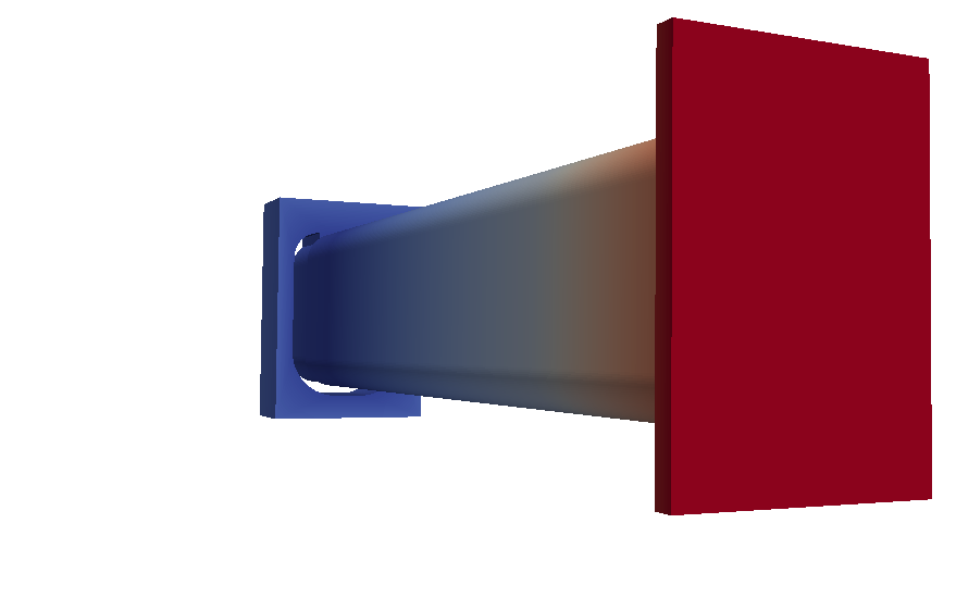
The beams of neutral atoms are produced by a complicated process which involves first accelerating a beam of ions and then neutralising the beam particles. Evidently, the acceleration stage must take place at a distance from the strong confinement fields in the main toroidal vessel. In a reactor design, there are also good radiological reasons for wanting complex engineered structures to be remote from the hot tokamak plasma. Hence the need for neutral beam ducts, see Figure 1. The duct walls will typically be defined using a CAD (Computer Aided Design) package, and may have a complex design to satisfy a range of different engineering constraints including the need for surface cooling. This complex geometry is ultimately represented in CAD geometry database using a special kind of spline function, known as a NURBS, for non-uniform rational B-spline [2].
Ideally the ducts are narrow enough to minimise the evacuated volume, yet allow passage of the neutral beam from their point of production into the central torus without hindrance. There are typically two sources of gas within the duct, ions escaping from the tokamak plasma and gas collected in the duct walls that is released by the beam’s impinging upon it. If the former source dominates, gas density will decrease away from the duct’s joint with the torus. Interaction between the beam and the background gas will ionise a fraction of the neutral beam particles and, under the influence of the tokamak magnetic field, these particles are likely to impact the duct wall and deposit a significant amount of heat. The initial aim of the SMARDDA development is to quantify power deposition on the wall, both from reionised particles, and from direct impact by the fast neutrals on the outskirts of the beam. A companion paper [3] describes application of SMARDDA-based software to the calculation of power deposited by a tokamak plasma on limiters and divertors.
I-B Related problems
There are two main problems to be treated by SMARDDA. The first is the tracking of charged particles in magnetic fields, corresponding to the motion of the reionised particles in the stray field in the duct. The second is to test particle paths for intersection with geometry, corresponding to the interaction of either the charged or neutral particles with the duct walls. To get good particle statistics in order to calculate power deposition accurately, it is desirable to solve these problems in as efficient a way as possible consistent with the likely accuracy of both the computed field and the designed surfaces.
Mathematically, the first problem is about the solution of ordinary differential equations (governing single particle motion) defined by discrete field samples (meaning the magnetic field is the result of a separate numerical calculation returning values on a separate grid). The second problem reduces to the ray-tracing problem, the efficient calculation of the intersection of a straight line segment with complex geometry. This is potentially the biggest cause of inefficiency, since the direct approach of comparing the particle trajectory with every part of the geometry gets very costly when for example, the geometry is defined by small elements and tracks have to be tested for intersection.
The above mathematical problems arise in a number of previously studied situations from which potential insights into the choice of best numerical algorithm for a new software development may be gathered. The two problems arise in combination for the computation of the efficiency of electron guns Section I-B1 and of the motion of tracer particles in a fluid flow, although there seems to be very little published on the latter problem. The second, ray-tracing problem, arises by itself both in neutronics, in the calculation of neutron trajectories through reactor shielding, and most obviously in computer graphics, in the visualisation of complex objects using computer display equipment. Moreover, the computer graphics literature is generous in publishing details of algorithms, a distinct advantage for taking ray-tracing techniques from this field and applying them to others.
I-B1 Electron guns
In gun codes [4], a charge distribution is calculated by tracking electrons from emitter to dump, then recalculating the electron trajectories in the resulting electric field to give a new charge distribution and so on until a consistent solution is achieved. In PIC or ‘particle-in-cell’ simulation [5, 6] of electrostatic devices such as electron guns, the charged particle paths are normally computed using the “Boris” scheme [5], a leapfrog scheme which is second-order accurate in both space and time as well as being symplectic, ie. having excellent conservation properties. Unfortunately, Auerbach and Friedman [7, 8] have discovered curious resonance type effects using a fixed timestep. Use of an adaptive scheme, whereby timestep size is changed to meet accuracy requirements, is however likely to mitigate the effect.
Electromagnetic field values are calculated by direct product spline interpolation between grid values of the fields, often a linear interpolation formula is used. The resulting curved trajectories are typically modelled as sequences of short straight lines or tracks, each corresponding to one timestep of the Boris particle advance algorithm.
Directly adopting this approach has several difficulties. The particles are tracked on the same computational grid which is used for calculating the fields. To ensure charge conservation, this grid is often a cuboidal lattice, and material boundaries are forced to coincide with the faces of the the grid cells or “voxels” (short for volume pixels). This makes for a ragged brick-like approximation to the geometry with consequently a highly inaccurate representation of the surface normals.
More recent PIC work [9, 10] has used unstructured grids, so that vacuum regions are filled irregularly with tetrahedral elements or “tets” rather than with uniform, hexahedral, voxels. The key idea [9, 11] is to use local coordinates within each “tet”, so that particles may be tracked efficiently and accurately across the grid. This concept was later employed in the CTLASS/MICHELLE software [12]. Unfortunately there is still a drawback for present purposes, in that the optimal grid spacing for the electromagnetic field may be very different from the optimal size of particle step, for example in the case of neutral particles.
I-B2 Neutronics
For deep shielding problems in neutronics, it is critical not to lose any particles due to small, round-off level, mistakes in the meshing, because the entire radiation flux may result from as few as three critical particles. Treatment of this problem, as exemplified by the Monte Carlo N-Particle (MCNP) software [13], requires representing the geometry by using the CSG (Constructive Solid Geometry) representation, ie. by intersecting a set of primitive quadric solids such as ellipsoids and tori. CSG has the advantage that particles may be located in cells defined by typically a small number of intersecting solids. This representation enables a ‘belt and braces’ approach to the movement of particles, because a surface intersected by a track must form part of the definition of the two cells in which the track starts and ends. Provided there are no mistakes in the geometry definition, it is plausible that less than one track in is lost due to round-off errors assuming a double precision numerical representation accurate to or so decimal digits. It is unclear that this extreme ability is strictly necessary in duct problems or indeed many others where the motions of many particles are likely to share similar properties.
Of relevance to the present study is the ability of MCNP and similar software to treat particle interactions such as absorption with a background medium. This leads to the reionisation algorithm described in Section III-C below.
I-B3 Plasma neutral transport
The DEGAS software [14] tracks a gas usually consisting of thermal neutrals through a volume meshed with tetrahedra. Unlike the PIC work described above, local coordinates are not used, but a ‘belt and braces’ like in the neutronics work is employed.
I-B4 Computer graphics
Computer graphics software must for most purposes operate in real-time, a typical example’s being the ability to spin an illuminated complex geometrical shape for the user to visualise. Most algorithms which compute detailed views on computer display equipment operate by following rays from the user’s (virtual) screen to the geometry and ultimately to a light source [15]. (This technique corresponds to the adjoint approach in neutronics.) Of the three different problems described in this section, ray-tracing is easily the most tolerant of error, since the human eye can easily compensate for an error rate of in pixels.
For computer graphics, the importance of speed results in a discretisation of the geometry which is as simple as possible, namely as a set of triangles to represent all the surfaces in the scene. Ray-tracing can then be reduced to a vast number of repeats of a very simple problem, namely to intersect a straight-line segment with a triangle, so that for example the repetitive parts of the algorithm can be implemented in hardware.
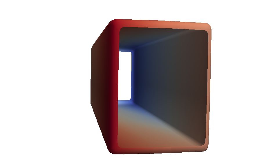
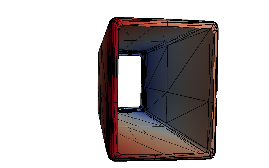
Nonetheless it is helpful to reduce the number of triangles which need to be tested against a particular track. This is achieved by use of auxiliary data structures, of which there are three main types. The first, called SEADS (Spatially Enumerated Auxiliary Data Structure) uses the voxel concept introduced in Section I-B1. To each voxel is associated a list of the surface triangles which intersect it. The idea is that the voxels which a track crosses may be cheaply found and the track tested only against those triangles corresponding to the relevant part of the SEADS. The other two auxiliary data structures by which the triangles are indexed are hierarchical data structures (HDS), eg. the octree divides the computational domain first into eight equal cuboids, but then only selectively subdivides these first cuboids into eight, and so on recursively, depending on details of the scene, see the projections in Figure 2. Parts of the octree which the track intersects are identified by a recursive algorithm and then the corresponding triangles are tested for intersection. For the HDS in particular, it might be expected that only of order objects need be tested for intersection with a given track. However, Chang [16, 17] describes how, for specific, selected distributions of objects in a scene, both SEADS and HDS may still require intersection tests.
II SMARDDA Ray-Tracing
Whilst the mathematical problem of calculating the charged particle motion can be regarded as solved by use of the Boris algorithm, its requirement to use a regular mesh is challenging for efficient solution of the mathematical ray-tracing problem to compute particle collision with the wall. A further constraint is provided by the need to discretise the NURBS-based geometry produced by CAD packages. To minimise effort, this is best achieved by meshing with pre-existing software, but meshing packages have their own limitations. There seems to be little software available to mesh NURBS consistently with a uniform cuboidal lattice, and the CSG representation that uses solids is fundamentally unable to treat the surface representation (“B-rep”) normally implied by use of NURBS. Thus an approach that involves the meshing of B-rep NURBS is indicated. Demand from the finite element community means that there a range of software to produce good tetrahedral meshes from NURBS. Since tet meshers normally commence by triangulating the surfaces, which is a technically easier problem, this implies a widespread capability to triangulate NURBS.
The literature reviewed above contains no algorithm which is able to treat efficiently straight particle trajectories which are both very long, in the case of the fast neutrals, and relatively short, in the case of the reionised particle motions over one timestep. The need to treat long trajectories argues against use of tet meshes, since many tets will have to be crossed, and in favour of working with the surface triangulations. This motivates the development of a new ray-tracing algorithm which incorporates many of the ideas from the computer graphics literature.
II-A SMARDDA Algorithm
The SMARDDA algorithm (pronounced “smarter”) is so named because it represents a hybrid of two distinct ray-tracing algorithms which respectively use the octree HDS and SEADS. The SMART algorithm for ray-tracing using an octree is described in a paper [18], generally regarded as difficult to understand, and the DDA (Digital Differential Analyser) algorithm uses SEADS [19, 20]. The DDA represents an efficient algorithm to advance a track long compared to cell size through a SEADS cell-by-cell, in much the same way as a charge-conserving PIC algorithm is required to do. The present section outlines the combined algorithm, mathematical details of key parts of SMARDDA are presented in Section II-B3 and the Appendix. A hybrid of SEADS and with a different, binary-spaced partition HDS has been examined by others [21].
The dimensions of the smallest cuboid in the octree can be used to “quantise” the position of a particle, ie. to assign to it coordinates that each are a multiple of the corresponding cuboid side. By translating the physical coordinates if necessary, it may be arranged that the origin of geometry is close to the zero of the quantised coordinates, so that all particles within the geometry have positive coordinates, each coordinate filling a large interval such as . A key part of the SMART algorithm is the realisation that the binary arithmetic operation of exclusive-or can then be used to locate particle positions relative to the octree. In particular, this leads to a simple test as to whether the positions at the start and end of a track are in the same octree cuboid.
The same-cell test is best illustrated by example, but see also Section II-B. Suppose say that two of the particle coordinates have identical integer part, so as to reduce the comparison to a 1-D problem, and further suppose that the octree cell is of size . The test is to shift out the trailing binary digits of each integer-truncated particle position, then apply the bit exclusive OR function of FORTRAN called IEOR on the remaining bits. For, consider the binary integer representations of three points
Supposing that the positions of the particle at the track ends are and , shifting the bits and applying IEOR as indicated above gives zero, indicating the positions occupy the same cell, but not so for the positions and .
The key idea in SMARDDA is that, having constructed an octree to index the objects in a scene, rays or tracks can be followed through the smallest cuboids at the deepest levels of the octree in a sequential manner analogous to the DDA algorithm, as explained further in the Appendix. An important refinement of the algorithm is to use a multi-octree structure to treat elongated physical structures as explained in the next Section II-B.
II-B Multi-octree
II-B1 Description
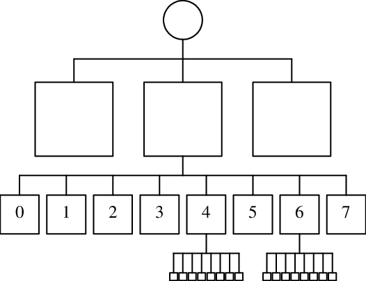
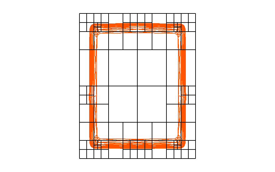
The octree is a widely used data structure, but it should be evident that it may become suboptimal for representing duct geometry which is almost by definition, elongated in one coordinate direction. This anisotropy has motivated the definition of the multi-octree, essentially the introduction of an additional hierarchical level to contain octrees, see Figure 3. Essentially the geometry can be thought of as encompassed by a brick built out of a set of smaller, identical octree bricks arranged in a rectangular array. In the case of a duct aligned along the -axis it is probable that and will approximate the duct aspect ratio. The size of each brick is chosen such that the volume does indeed encompass all the geometry.
The next step involves producing an octree indexation of the CAD surfaces or more precisely their triangulations, within each cuboid. This is implemented as a two-stage process. The first stage uses the classic octree recursion and termination criterion [15]. Cuboids containing triangles are identified [22] and inspected, and where necessary the cuboids are divided into eight to reduce the number of triangles they contain. This process continues recursively until each contains a maximum specified number of triangles, typically is found to give good results. There are the important details that
-
1.
Before indexing starts, coordinates are quantised using the vector , defined by where normally .
-
2.
It is necessary to recognise the case where further subdivision does not reduce the number of triangles within a cuboid (typically this occurs when the cuboid is smaller than the triangles).
Suppose that the above algorithm leads to a depth of octree, meaning that the number of levels in the resulting octree, excluding the ‘root’ (see the lower part of Figure 3) is . This octree construct is then revised as follows: every cuboid is examined to see whether it is empty or not, and if not, subdivided into eight, but no lower levels than are allowed. Empty cuboids are indicated by a nodal marker. whereas each non-empty cuboid has an associated “linked list” of the triangles which intersect it.
II-B2 Advantages of the multi-octree
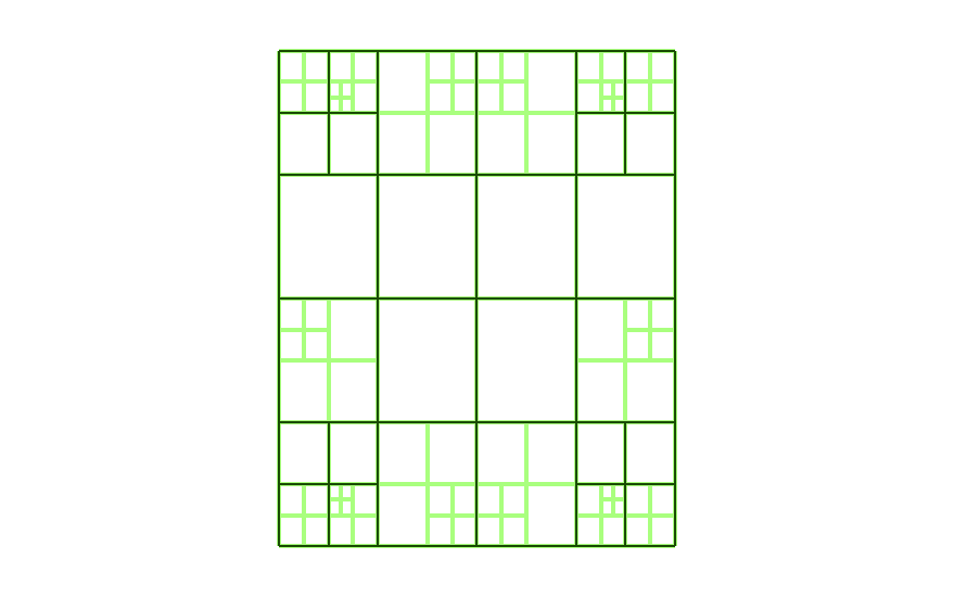
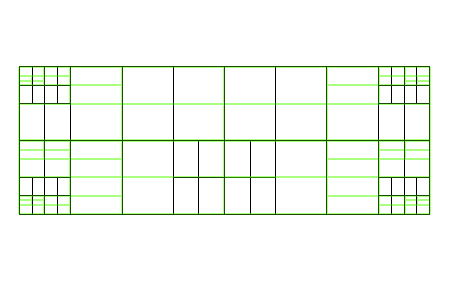
Figure 4 shows the octree and multi-octree which result from application of the above algorithm to a relatively coarse meshing using triangles of the indicative duct shown in Figure 2. The standard octree has cuboidal cells whereas, for the same parameters, the multi-octree has only . For the SMARDDA algorithm generally, this is expected to result in an approximately proportionate computational speed-up, but for application to the duct problem see Section IV-A.
A further advantage is derived from the quantisation of the positions . Suppose the quantised or integer vector corresponding to is given by , so that (possibly following a vector translation)
| (1) |
Suppose further that each of and is represented in terms of its bit representations in a -bit integer word. Assignment of position in each coordinate to the octree then proceeds as follows.
-
1.
The first group of bits on the left (most significant bits), addresses the octree in which the vector lies, so that extracting this group from each of and gives the location in -space.
-
2.
Mask the bit representations to hide this first group, then form the most significant unmasked bit in each component into a bit-vector that indicates in which of the eight cuboids at the next level the vector lies.
-
3.
Descend the tree to the node corresponding to this cuboid, then use the next most significant unmasked bit in each component to descend again and so on until a terminal node or “leaf” corresponding to an undivided cuboid is found.
To illustrate point (2) about the bit-vector, referring to the node labels in Figure 3, since , node 3 contains the cuboid in position relative to the parent node in coordinates.
Hence the tree structure may be descended very economically to termination, by a combination of bit-masking and bit-shifting functions operating on integers.
II-B3 Same-Cell Test
The movement within an octree described at the end of the preceding Section II-B2 draws heavily from the SMART algorithm [18]. The same ideas may be applied to the problem of determining whether the two ends of a particle track lay in the same cell. Suppose the coordinates of the two points are truncated to integer values, to give two integer vectors . Evidently, and hence the two end-points occupy the same cuboid of side , if their bit representations are the same except in the last bits. Or, equivalently, in more mathematical language
| (2) |
where ISHFT is the bit shift function which is defined so as to move bit patterns to the right for positive argument, hence the minus sign, and IEOR is the exclusive-or function introduced earlier.
In many cases, the second end-point will turn out to lie within an adjacent node, and this case is treated specially for efficiency, as follows, by computing the vector with components
| (3) |
(which are anyway needed in the calculation of the sum Eq. (2) above). If for a given , then the two binary vectors have the same parent node but they occupy different child nodes, and the index vector for differs from that of by the vector with components where the sign taken is that of .
III Duct CAD and Physics
As indicated, SMARDDA expects geometry to be presented as a set of possibly millions of triangles. To give a well-defined interface the legacy vtk file format [23] is used. It has the advantage that file contents are easily visualised using the freely available ParaView software [24]. As its name implies the legacy vtk file format has remained unchanged for many years, and is likely to remain current because a good deal of software, including now SMARDDA, relies upon it. The question of CAD to vtk conversion for the duct problem is now addressed.
III-A CAD Conversion
The output from a CAD package is seldom suitable for use by physics software. Invariably, there is too much detail. In the context of duct modelling, only surfaces matter and small screws, bolts and other small features are unimportant provided they are flush or recessed. However, unintentional small gaps which are insignificant on an engineering scale may be disastrous in allowing computed rays or particles to escape the domain. Both these are long-standing issues for finite element engineering packages and many options are commercially available for CAD defeaturing and repair.
The solution adopted relies heavily on the well-known CATIATM CAD system supplied by Dassault to perform much of the defeaturing. The CADfixTM package supplied by ITI TranscenData is largely dedicated to defeaturing and repair, and can work with CAD from many different vendors, including CATIA files. Thus it is possible for a user without training in CATIA to make final adjustments and repairs to CAD produced using CATIA, then use the inbuilt CADfix mesher to produce a suitable surface mesh of triangles. Locally written software then interrogates the resulting geometry database and produces the vtk file. A separate code generates the HDS together with the quantising position vector transformations.
III-B Neutral Launch
The neutral beam input is modelled as a set of one or more beamlets each with a Gaussian cross-section. Let denote the energy of particles in beamlet which has a total power of . Supposing without loss of generality that the beam is directed close to the -direction, then the centre of each beamlet is specified by co-ordinates in a plane , with its spread given standard deviations . It follows that particles crossing at position have weights proportional to
| (4) |
Neutral particles are launched from so as to sample each beamlet. Quasi-Monte-Carlo sampling is employed, specifically a 2-D Halton sequence composed of sequences of vectors with components given by Van der Corput sequences of base and base respectively, cf. the “quiet start” technique used in PIC codes [6]. Van der Corput sequences contain numbers on the unit interval generated using the reversed bit patterns of the positive integers [25]. A Halton sequence is completely deterministic from which fact derive better sampling properties than the more usual Monte-Carlo technique, yet there is no need to set the length of a Halton sequence in advance unlike with homogeneous sampling techniques. This simplifies the launch of additional particles if additional sampling is indicated by the results of an initial run.
III-C Reionisation and Reionised particles
The sources of fast ions in the duct are collisions with the background gas and charge exchange reactions between the neutral beam and ions in the gas. It will be assumed for simplicity, and to give a worst case scenario, that the gas has a uniform density , although the case of variable density can be treated in a similar way [26].
To treat reionisation, the preferred approach is to use particle weighting. The beam particles in any event are weighted by to reflect the Gaussian distribution of number density in each beamlet, now the reioinised particles are given a weight according their local rate of formation. If the neutral beam particle trajectory is considered as traversed in small timesteps of duration , then
| (5) |
where is the re-ionisation cross-section and speed , with equal to the mass of beam particles and is the charge on the electron if is measured in electron-Volts (eV).
The above algorithm results in the production of ionised particles, each assumed to have the velocity of the impacting neutral. The ions are assumed to travel to the duct walls without further particle interactions, under the the Lorentz force law in the static magnetic field , viz.
| (6) |
where is the particle’s position, is its velocity and denotes time. The numerical details of the trajectory integration are standard [5, § 4-7-1] given a definition of in terms of samples on a uniform rectilinear grid. To test for wall collisions, the ion trajectory is assumed to consist of short straight tracks joining the positions at the start and end of each timestep.
IV Results
The ITER duct of Figure 1 is converted as described in Section III-A to give a vtk file with triangles that represents the surfaces. Since the imported duct geometry is so elongated in the -direction, this is an interesting configuration for testing the effect of variations in the -size of multi-octree. Note that a -multi-octree corresponds to the classical octree. It was rapidly discovered that it was not possible to produce octrees of depth ten or less without setting or so, apparently because of the inhomogeneity of the surface meshing. However, comparatively simple multi-octrees with – cells were produced with a maximum of – triangles per cell, see Table (I) in Section IV-A.
IV-A Ray Statistics
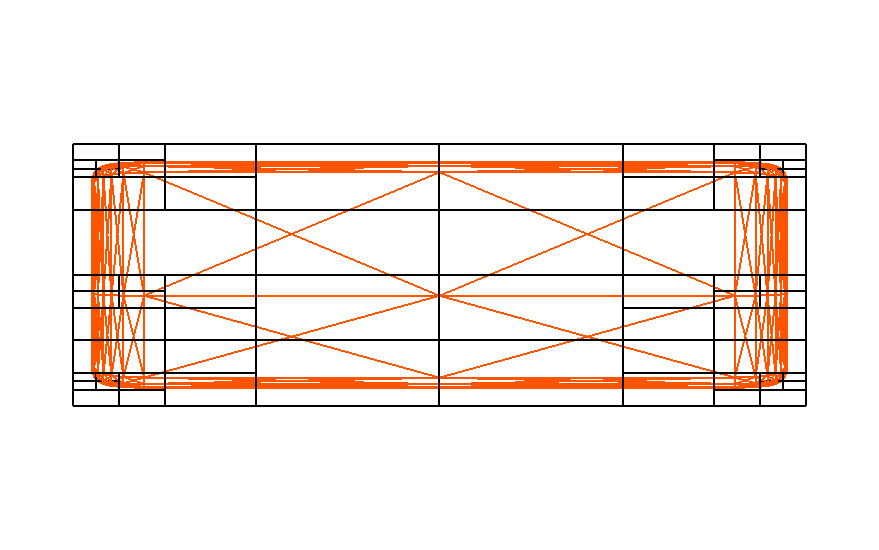
As part of the testing process, a “beam” of neutrals was arranged to be launched from a single point in the duct centre, to fill uniformly a cone of angle about the long duct axis. Two sizes of were employed, corresponding to a spread in degrees of approximately , and giving of spread. The smaller spread is chosen to be indicative for a neutral beam which fills the duct, the larger spread is designed to generate a significant number of collisions with with the duct walls as undergone by the fast ions which strike and heat the wall, see Figure 5.
Each of the tests recorded in Table (I) involves the launch of particles. Hence it will be seen that each track intersection test takes of order a few micro-seconds. The variation in cpu time with HDS is significant. It is evident that the fastest tracking occurs when the number of octree cells along the duct is least. This is most evident when the tracks are more nearly parallel to the duct for . Placing more cells along the duct is evidently beneficial when tracks are directed more across the duct as in the case.
No particle tracking algorithm is perfect, because ultimately round-off error causes in the duct problem, some tracks to miss geometry they should have intersected. For the cases described in Table (I), anomalous tracks were detected by visual inspection of the plot of end-points each drawn with a large size. When , a single anomalous track was detected for the octree HDS, but all tracks were computed successfully for the other HDS. The wider beam is more demanding test of the surface intersection algorithm, but Table (I) shows that the anomalous loss rate is less than in for most cases. This is probably a good rate for a computer graphics-based algorithm which could easily lose one track in without the viewer’s noticing. In fact from the distribution of anomalous points, it is clear that they are associated with octree faces and much smaller anomalous losses might be easily achievable. However, the present loss rates are compatible with very accurate calculations of power deposition in the duct.
| cpu- | cpu- | Lost | ||
|---|---|---|---|---|
IV-B Power deposition
The power deposited in the ITER duct of Figure 1 may be calculated using SMARDDA. Representative parameters are assumed for the neutral beam, viz. total power of MW and keV. The beam is assumed to consist of a single Gaussian beamlet centred in the middle of the duct with m, m. A high background gas density m-3, approximating that of the tokamak edge is assumed, and is assumed to present a cross-section for re-ionisation m2 to the beam. A representative magnetic field is applied that reaches approximately T at the torus end of the duct.
The beam is sampled using particles and the trajectory of each neutral generates ions, so that the total number of particles followed is requiring tracks to be tested for geometry intersection. No aberrant particles are found and the computation completes in under an hour on a laptop, ie. a cpu cost of ms/track. The resulting power deposition profile for the top of the duct is shown in Figure 6. The results are easier to interpret than those from older software which takes a week of cpu [1].
Acknowledgment
This work was funded by the RCUK Energy Programme grant number EP/I501045 and the European Communities under the contract of Association between EURATOM and CCFE. To obtain further information on the data and models underlying this paper please contact PublicationsManager@ccfe.ac.uk. The views and opinions expressed herein do not necessarily reflect those of the European Commission. [Details of the SMARDDA Algorithm] The SMARDDA algorithm is encapsulated as a function which takes a straight particle track, specified by its start and end points, and determine whether it intersects any part of the geometry. If so, it returns the first point of intersection. The track is defined by two arguments of type posnode, a type which consists of a position vector and the identifier of the deepest corresponding node in the octree. Frequently, the node of the start position is known as the result of a previous calculation, if not, as occurs typically on the first step, it is calculated by binary look-up in the octree. The second argument will acquire a nodal value only upon exit, corresponding to the end of the track. Its position vector will be changed from the input value only if the track intersects the geometry as signalled by the return of another, the last, function argument.
The function uses the same-cell test of Section II-B3 as a preliminary check. This is efficient when particle trajectories are short. For longer tracks, the particle advance is controlled by a loop in the first coordinate . For reasons which will become apparent, particle track is started from a virtual origin, viz. an integer (quantised) position in the first coordinate, either the largest integer less than the start position if the motion is forwards, or the smallest integer greater than the start position if motion is backwards, see the illustration in Figure 7.
In the DDA applied conventionally to a SEADS, each subsequent increment of the integer loop counter gives a position in a different cell along the track. Supposing that lateral motion of the particle relative to the first coordinate direction is negligible, the first position coordinate is incremented by one when motion is forwards, or decremented by unity when motion is backwards. First, the track is tested against objects in the cell indexed by the octree node corresponding to the start position, and if there is a collision “in the node”, the track terminates at the intersection point. If there is no collision, there is a same-cell test of the new position and the end-point of the track. If this is true, the loop terminates, otherwise the position is updated and the loop continues in a new cell with collision tests etc.
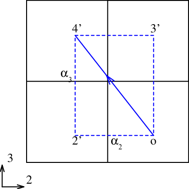
The advance along the track is complicated in higher dimensions because the track may enter new nodes as a result of its motion in the other coordinates. It is efficient to arrange so that the particle moves farthest in the direction of the first coordinate, by relabelling if necessary. The other two coordinates may be chosen purely so that the relabelled coordinates form a right-handed set. In the resulting (quantised) coordinate system, the vector of advance is where , and . In outline, coordinate is incremented by to see whether this point lies in a new node, then coordinate is incremented by and this point tested, and finally all three coordinates are updated, and the new point tested. The latter point now on the track, is then updated like the first virtual point, and so on.
In detail, consider first the update. There is a quick test as to whether the integer part of has changed, then if so, a test whether the new position, shown as point in Figure 8, lies in the current node. If is found to lie in a new node, the objects in that node are tested for collision with the track, and if no collision is found, the code proceeds. The coordinate is updated to give the point , which of course may lie in a new node, and if so, the node is tested for collisions in the same way. There is the additional complication that the point may lie in a node different to that of either of the points and . If so, a further test for collision is performed in this third node. However, this is the maximum number of nodes that need testing between updates of .
Moreover, and distinguishing the SMARDDA algorithm from the DDA variant above, the increment in unity of the position is replaceable by increments which could be as large as , , or more. The idea is to jump along the track as far forwards in the current cell as possible, to an integer point , such that the next integer increment of will produce a point in a new cell, possibly laterally displaced.
The underlying mathematics are as follows. For DDA it is anyway convenient to introduce binary markers which are unity for forwards motion in direction and zero for backwards. Supposed the quantised size of the cell is where labels the octree level, then if are the coordinates of the current cell’s origin, the path increment can be calculated using
| (7) |
as
| (8) |
(The last term corresponds to a displacement limited by the cell size, and the second-last accounts for a track ending at .) One step of the DDA algorithm can then be applied as though beginning from the position
| (9) |
but note the need for special treatment at the track end-point. The concept of virtual origin is important here, in that the track can be tested in sections defined by a sequence of virtual origins each corresponding to an integer value of .
Last details are that the testing of the track for collisions is performed using Badouel’s algorithm [27], modified to take into account finite precision computer arithmetic as in ref [10]. Where the point of intersection of the track with the object face is needed, eg. for diagnostic purposes, it is computed as in the second step of Badouel’s algorithm [27, 10].
References
- [1] D. King and W. Arter, “Particle tracking in complex geometry,” in 21st International Conference on Numerical Simulation of Plasmas (ICNSP ‘09). IPFN, 2009, pp. 37–38, http://icnsp09.ist.utl.pt/code/preview.php?abs_id=48.
- [2] G. Farin, Curves and surfaces for computer aided geometric design. Academic Press Professional, Inc. San Diego, CA, USA, 1990.
- [3] W. Arter, E. Surrey, and D. King, “The SMARDDA Approach to Ray-Tracing and Particle Tracking,” IEEE Transactions on Plasma Science, vol. Submitted, 2014.
- [4] W. Hermannsfeldt, “EGUN-an electron optics and gun design program,” SLAC, Tech. Rep. SLAC-R-331, 1988.
- [5] R. Hockney and J. Eastwood, Computer Simulation Using Particles. IOP Publishing, 1988.
- [6] C. Birdsall and A. Langdon, Plasma Physics Via Computer Simulation. Taylor & Francis, 2004.
- [7] A. Friedman and S. Auerbach, “Numerically induced stochasticity,” Journal of Computational Physics, vol. 93, no. 1, pp. 171–188, 1991.
- [8] S. Auerbach and A. Friedman, “Long-time behaviour of numerically computed orbits: small and intermediate time-step analysis of one-dimensional systems,” Journal of Computational Physics, vol. 93, pp. 189–223, 1991.
- [9] F. Assous, P. Degond, and J. Segre, “A particle-tracking method for 3D electromagnetic PIC codes on unstructured meshes,” Computer Physics Communications, vol. 72, no. 2-3, pp. 105–114, 1992.
- [10] A. Haselbacher, F. Najjar, and J. Ferry, “An efficient and robust particle-localization algorithm for unstructured grids,” Journal of Computational Physics, vol. 225, pp. 2198–2213, 2007.
- [11] D. Seidel, M. Pasik, M. Kiefer, D. Riley, and C. Turner, “Advanced 3D electromagnetic and particle-in-cell modeling on structured/unstructured hybrid grids,” Sandia National Labs., Albuquerque, NM (United States), Tech. Rep. SAND–97-3190, 1998.
- [12] J. Petillo, E. Nelson, J. DeFord, N. Dionne, and B. Levush, “Recent developments to the MICHELLE 2-D/3-D electron gun and collector modeling code,” IEEE Transactions on Electron Devices, vol. 52, no. 5, pp. 742–748, 2005.
- [13] X-5 Monte Carlo Team, “MCNP-A General Monte Carlo N-Particle Transport Code, Version 5 - Volume I: Overview and Theory,” Los Alamos, Tech. Rep. LA-CP-03-1987, 2003.
- [14] Stotler, D. and Karney, C., “Neutral gas transport modeling with degas 2,” Contributions to Plasma Physics, vol. 34, no. 2-3, pp. 392–397, 1994.
- [15] A. Watt and M. Watt, Advanced animation and rendering techniques. ACM Press New York, NY, USA, 1991.
- [16] A. Chang, “A survey of geometric data structures for ray tracing,” Polytechnic University, Brooklyn, Tech. Rep., 2001.
- [17] ——, “Theoretical and experimental aspects of ray shooting,” Ph.D. dissertation, Polytechnic University, Brooklyn, 2004.
- [18] J. Spackman and P. Willis, “The SMART navigation of a ray through an oct-tree,” Computers and Graphics, vol. 15, no. 2, pp. 185–194, 1991.
- [19] A. Fujimoto, T. Tanaka, and K. Iwata, “Arts: Accelerated ray-tracing system,” IEEE Computer Graphics and Applications, vol. 6, no. 4, pp. 16–26, 1986.
- [20] P. Hsiung and R. Thibadeau, “Accelerating ARTS,” The Visual Computer, vol. 8, no. 3, pp. 181–190, 1992.
- [21] B. Pradhan and A. Mukhopadhyay, “Adaptive cell division for ray tracing.” Computers and Graphics, vol. 15, no. 4, pp. 549–552, 1991.
- [22] T. Akenine-Möller, “Fast 3D triangle-box overlap testing,” Journal of Graphics Tools, vol. 6, no. 1, pp. 29–33, 2002.
- [23] Kitware, The VTK User’s guide. Kitware Inc., Colombia, 2006, ch. File formats for VTK version 4.2, http://www.vtk.org/VTK/img/file-formats.pdf.
- [24] A. Henderson, ParaView Guide, A Parallel Visualization Application. Kitware, 2007.
- [25] H. Niederreiter, Random Number Generation and Quasi-Monte Carlo Methods. Society for Industrial Mathematics, 1992.
- [26] F. Brown and W. Martin, “Direct Sampling of Monte Carlo Flight Paths in Media with Continuously Varying Cross-sections,” in ANS Mathematics and Computation Topical Meeting, Gatlinburg, TN, April, 2003, pp. 6–11.
- [27] D. Badouel, “An efficient ray-polygon intersection,” in Graphics Gems, A. Glassner, Ed. Academic Press Professional, Inc. San Diego, CA, USA, 1990, pp. 390–393.