Abstract

Quantum cosmology implies corrections to the classical equations of motion which may lead to significant departures from the classical trajectory, especially at high curvature near the big-bang singularity. Corrections could in principle be significant even in certain low-curvature regimes, provided that they add up during long cosmic evolution. The analysis of such terms is therefore an important problem to make sure that the theory shows acceptable semiclassical behavior. This paper presents a general search for terms of this type as corrections in effective equations for a $k=0$ isotropic quantum cosmological model with a free, massless scalar field. Specifically, the question of whether such models can show a collapse by quantum effects is studied, and it turns out that factor-ordering choices in the Hamiltonian constraint are especially relevant in this regard. A systematic analysis of factor-ordering ambiguities in effective equations is therefore developed.

1 Introduction

Effective equations are useful tools to analyze quantum theories by adding suitable correction terms to classical equations, for instance by using equations of motion for expectation values of operators of interest. Just like expectation values, effective equations that describe their evolution depend on the states or class of states whose evolution is being approximated. The low-energy effective action often used in particle physics, as perhaps the best-known example, describes quantum corrections for states near the vacuum of the interacting theory. For other states, different quantum corrections arise. Effective equations are state-independent only in rare cases such as free theories or the harmonic oscillator, when no quantum back-reaction and therefore no dynamical quantum corrections occur. Such systems also exist in (loop) quantum cosmology, where they play a similar role as the base order for perturbation theories when interactions are present [1].

As an example for potentially large perturbative effects in quantum cosmology, it has been suggested that classically ever-expanding models could eventually collapse due to quantum corrections [2]. Such a feature is unexpected because the more the universe expands, the more classical it is supposed to become, with quantum corrections playing smaller and smaller roles. However, with long evolution involved, small quantum effects could potentially add up and eventually drive the universe into collapse even in semiclassical regimes. As shown in [2], the outcome depends on what semiclassical quantum state is realized and how its fluctuations of different variables change in time. To test the proposed scenario, one needs information about dynamical semiclassical states over long evolution times, an issue that requires good control on quantum evolution and, when addressed with effective equations, a systematic scheme of going beyond the leading classical order.

The effective equations used in [2] (as well as [3]) were an extension of the classical limit obtained from methods provided in [4]. This scheme of going beyond classical order, however, is not entirely systematic because assumptions about the evolving state must be made; they have not been self-consistently derived within the scheme. For this reason, the suggested collapse remained a possibility but could not be demonstrated firmly. (Note that going to the other extreme, the high densities of the big bang, requires even better control of evolving states no longer required to be semiclassical. For this reason, the high-curvature regime of quantum cosmology remains poorly understood, even though rather definite-looking statements are sometimes attempted.) In this article, we use a systematic perturbative framework to derive information about effective equations and dynamical semiclassical states and see whether the suggestions of [2] can be realized. We will be led to a more systematic look on factor-ordering ambiguities than provided so far.

2 Modified Friedmann equation, recollapse, and factor ordering

Although the low-curvature regime can be formulated in Wheeler–DeWitt quantum cosmology [5] and does not require additional corrections and modifications from extensions such as loop quantum cosmology [6, 7], we will follow [2] and use the latter for a general discussion. This choice also helps us keep our notation close to that of [2]. In brief terms, loop quantum cosmology of spatially flat isotropic models proceeds by formulating the Friedmann equation in canonical variables $c=\gamma\dot{a}$ and $|p|=a^{2}$,

$$-\frac{3}{8\pi G\gamma^{2}}c^{2}\sqrt{|p|}+H_{\rm matter}=0\,,$$ (1)

and modifying it by using periodic functions of $c$ (or, as seen in more detail below, $\delta(p)c$ with some function $\delta(p)$) instead of $c$. In this way, one mimics the fact that the full theory of loop quantum gravity [8, 9, 10] provides operators only for holonomies of the connection corresponding to $c$, not for the SU(2)-connection itself [11].

The (almost) periodic nature of functions substituting $c$ is motivated by a reduction of the internal gauge freedom from SU(2) to U(1) when isotropy is imposed [12]. Recent attempts to bring about a closer relation between minisuperspace models of loop quantum cosmology and the full theory have questioned the almost periodic nature of isotropic holonomies as a reliable feature of loop quantum gravity [13], as a consequence of crucial differences between Abelian and non-Abelian treatments [14]. In this paper, we aim to investigate a question that can be posed within pure minisuperspace models, whose form and quantum modifications we will take for granted. We are not claiming that the features analyzed are in any way related to the full theory of loop quantum gravity.

Such a modification to

$$-\frac{3}{8\pi G\gamma^{2}}\frac{\sin(\delta(p)c)^{2}}{\delta(p)^{2}}\sqrt{|p|}+H_{\rm matter}=0$$ (2)

is most relevant in regimes where $\delta(p)c$ is large (at large curvature). If one expands the sine function, terms beyond the classical ones may be interpreted as contributions to higher-curvature terms. (They are not complete as higher-curvature corrections, however, because higher time derivatives have not been included. The latter would result from quantum back-reaction [15, 16].) From equations of motion generated by (2) used as a Hamiltonian constraint in proper-time gauge, one finds that the modified Friedmann equation in terms of $\dot{a}$ or $H=\dot{a}/a$ takes the form

$$H^{2}=\frac{8\pi G}{3}\rho\left(1-\frac{\rho}{\rho_{\mathrm{QG}}}\right)$$ (3)

with $\rho_{\rm QG}=8\pi G/3\delta^{2}|p|$ [17, 18, 19, 20]. If one assumes $\delta(p)\propto 1/\sqrt{|p|}$ as in [19], $\rho_{\rm QG}$ is a constant and Planckian for $\sqrt{|p|}\delta(p)\sim\ell_{\rm P}$. This form makes it especially clear that the modification is relevant only at large density.

Loop quantum cosmology represents the modified constraint (2) as a difference equation [21, 22], obtained from shift operators $\widehat{\exp(i\delta(p)c)}$ acting on a wave function in the triad representation. From this difference equation or the underlying Hamiltonian-constraint operator, (2) can be reproduced as the “classical” limit by computing the expectation value in Gaussian states and ignoring all fluctuation-dependent terms [4]. From the point of view of quantum dynamics, the result is the classical limit because fluctuations and their back-reaction on expectation values are ignored. Still, the result does not agree with the classical equation (1) because loop quantum gravity implies quantum-geometry corrections in addition to the usual dynamical quantum corrections, which give rise to the modifiction (2) of (1). Only a combined classical and low-curvature limit [23] brings loop quantum cosmology fully back to the classical Friedmann equation (1). (See also [24, 25].)

The modification in (2) alone does not affect late-time evolution much. However, quantum evolution implies additional corrections, which in canonical models can be computed by quantum back-reaction of fluctuations and higher moments of a state on expectation values [26, 15]. The leading-order expectation value that gives rise to the classical limit must be expanded systematically to include these terms. Such terms were computed in [2], with potentially significant low-curvature implications. In addition to the usual quantum corrections on small distance scales, higher-order corrections may allow for the possibility of an expanding universe to collapse at large size when the energy density is suitably small, even in the absence of spatial curvature — a significant departure from classical theory. (The possibility of a recollapse was also conjectured in [27] by an alternative quantum Hamitonian scheme, as well as in [28, 29] by a coherent state functional integral approach. In the latter cases, assumptions on the asymptopic semiclassical behavior of coherent states were more restrictive.)

In [2], lacking a derivation of properties of dynamical semiclassical states, a suitable coherent state for large volume and late times had to be chosen, assumed, as in most cases, to be an uncorrelated Gaussian. With this choice, the classical-limit scheme of [4] was developed further to calculate fluctuations and expectation values. The end result is a modified Friedmann equation, which we write here as

$$H^{2}=\frac{8\pi G}{3}\rho\left[1-\frac{\rho}{\rho_{\mathrm{QG}}}\left(1+\bar{\epsilon}^{2}\right)+\frac{1}{2}\bar{\epsilon}^{2}-2\epsilon^{2}\frac{\rho_{\mathrm{QG}}}{\rho}\right]\,.$$ (4)

In this expression, $\epsilon$ is the quantum fluctuation of curvature or the Hubble parameter $H$, while $\bar{\epsilon}:=(\Delta\nu)/\nu$ is the relative volume fluctuation, using $\nu=a^{3}$. (Unlike $\bar{\epsilon}$, the latter is not invariant under a change of spatial coordinates or of $V_{0}$.) As mentioned, Eq. (4) was derived with a Gaussian ansatz for the wave function with zero correlations of the canonical pair $(H,\nu)$, for which $1/\epsilon$, the inverse curvature fluctuation, is proportional to the volume fluctuation $\Delta\nu=\nu\bar{\epsilon}$ thanks to the uncertainty relation.

The last term in (4) is especially important for the question posed here, because it has the lowest power of the energy density $\rho$. The equation has the correct classical form when all fluctuations are sent to zero first, and then $\rho_{\rm QG}$ to infinity. The semiclassical behavior, in which fluctuations are small but not zero, agrees with the classical one provided $\epsilon$ goes sufficiently fast to zero as the energy density decreases in an expanding universe. For a Gaussian state, $\Delta\nu$ would increase accordingly, but in (4) it is always suppressed by factors of $1/\nu$ in $\bar{\epsilon}$. Indeed, one can solve the quantum model in a specific factor ordering and find properties of dynamical coherent states [30]. In this harmonic quantum model, with the same classical dynamics, $\epsilon$ must decrease at low curvature and cannot remain constant, while $\bar{\epsilon}$ is asymptotically constant for any state [1]. This behavior may, however, change when the model is quantized with a different choice of factor ordering. The question is whether it is then possible for $\epsilon$ to decrease sufficiently slowly that the last term in Eq. (4) can cancel the others and enable a recollapse, where $H=0$ at large $\nu$.

In the present context, the important part to note from Eq. (4) is that at late time and large volume, for an expanding universe with suitably low energy density ($\rho\sim 2\epsilon^{2}\rho_{\mathrm{QG}}$), the universe could perhaps collapse. An inverse-$\rho$ quantum correction associated with $\epsilon$ in (4) may seem surprising. But one way of looking at this is by distributing the $\rho$ in front to see that the final term is independent of the energy density and only depends on the quantum fluctuations. It functions as a negative cosmological-constant term if $\epsilon$ varies slowly. When the energy density is of the order of those fluctuations, the final term dominates and could lead to collapse – depending on the exact quantum dynamics.

From the perspective of effective equations, the classical model quantized in [2] — a spatially flat isotropic model sourced by a free, massless scalar — is identical to a harmonic one, without any quantum back-reaction [1]. The only corrections to classical evolution are due to quantum geometry; no quantum back-reaction should occur. However, compared to [1], [2] used a different factor ordering of the quantum constraint as well as quantum-geometry modifications of inverse-triad type, not just holonomy corrections as in (2). These variations imply quantum back-reaction, which, thanks to the proximity to a harmonic model, should not be large but could still be significant after long evolution. In this paper, we explore the possibility of such a term in the modified Friedmann equation found by embarking on a systematic method of deriving effective equations, including the underlying properties of dynamical semiclassical states [26, 15]. By way of the example of collapse solutions, we will therefore study several implications of terms in effective equations, including the role of factor ordering. We will provide a general parameterization of these ambiguities in an expansion of the quantum-corrected Hamiltonian constraint by powers of $H$, which turn out to require inverse negative powers as well. These methods will require a shift in viewpoint, focusing on the form of the last term in (4) instead of the possibility of a recollapse which is difficult to assess in an expansion with negative powers of $H$. This fact highlights how subtle the semiclassical limit of quantum cosmology can be. In particular, it is not clear whether (loop) quantum cosmology has the standard semiclassical behavior even in isotropic models.

3 Quantum cosmology and effective equations

In spatially flat isotropic models, the basic pair of canonical variables is the extrinsic curvature $c=\gamma\,{\rm d}a/{\rm d}\tau$ and its conjugate $|p|=a^{2}$ where $\gamma$ is the Barbero-Immirzi parameter [31, 32] of loop quantum gravity, $a$ is the scale factor, and $\tau$ is proper time. The momentum $p$ is derived from an isotropic densitized triad and so can take both signs due to the triad orientation. The fundamental Poisson bracket is $\{c,p\}=8\pi G\gamma/3$ where $G$ is Newton’s constant as before. (As already mentioned, we assume the coordinate volume of our homogeneous region to equal one.) Beginning with the Friedmann equation for an isotropic and homogeneous background, we can write the Hamiltonian constraint in these canonical variables as (1) with $H_{\rm matter}=\frac{1}{2}|p|^{-3/2}p_{\phi}^{2}$ for a free, massless scalar $\phi$ where $p_{\phi}$ is the momentum conjugate to $\phi$ such that $\{\phi,p_{\phi}\}=1$.

3.1 The model

As this work is motivated by [2], we will use a similar notation for a direct comparison, and so by a canonical transformation we introduce new conjugate variables:

$$b\equiv\delta\frac{c}{\sqrt{|p|}}\quad,\quad\nu\equiv\frac{2}{3\delta}{\rm sgn}(p)|p|^{3/2}\quad\mbox{such that}\,\{b,\nu\}=8\pi G\gamma/3\,.$$ (5)

Here, $\delta$ is a length parameter that determines the size of holonomy corrections. Looking at large-scale evolution of large $|p|$, we are free to fix the sign of $p$ or $\nu$, from now on assumed positive. (These variables are a specific case of the general parameterization of [33], providing different cases of lattice refinement. While the harmonic model has a dynamics independent of the specific choice of basic variables where $\nu$ could be any power of $p$, quantum corrections in models that differ for instance by factor ordering depend on such parameters. Here, however, we confine ourselves to the choice made in [2] because our aim is to explore the scenario suggested there.)

In the new variables, the classical Hamiltonian constraint is

$$-\frac{9\,\nu b^{2}}{16\pi G\gamma^{2}\delta}+\frac{p^{2}_{\phi}}{3\delta\,\nu}=0.$$ (6)

We use the free scalar $\phi$ as an internal time variable; the monotonicity of $\phi(\tau)$ is guaranteed for the free case, and so evolution for $b(\phi)$ and $\nu(\phi)$ is governed by the Hamiltonian $p_{\phi}(b,\nu)$ which is found as a phase-space function by solving for $p_{\phi}$ in Eq. (6). Doing this, we have $p_{\phi}\propto|\nu b|$. (In Sec. 4.1 we discuss ambiguities related to the choice of internal time.)

The momentum $p_{\phi}(\nu,b)$ of internal time, as a function of the remaining degrees of freedom, acts as the Hamiltonian generating evolution. Since it is quadratic, the system is equivalent to a harmonic one, which, like the harmonic oscillator, can be quantized to a model without quantum back-reaction. However, in a model of quantum gravity there may be quantum-geometry corrections as well, changing the Hamiltonian not just by quantum back-reaction terms but also by more-severe modifications. In loop quantum cosmology, as one popular example, holonomy and inverse-triad corrections occur.

Holonomy corrections replace the $b$ in $p_{\phi}(\nu,b)$ by the non-linear $\sin(b)$, making the Hamiltonian non-quadratic in canonical variables. Nevertheless, as shown in [1], surprisingly, they do not remove harmonicity even upon quantization provided a suitable factor ordering is chosen: If we define $J:=\nu\exp(-ib)$, the new set $(\nu,J)$ of (non-canonical) basic variables satisfies a linear algebra under Poisson brackets, in which the linear Hamiltonian $p_{\phi}=|{\rm Im}(J)|$ is just the right holonomy-modified version of the internal-time Hamiltonian $p_{\phi}$. These properties are preserved when the model is quantized with Hamiltonian $\hat{p}_{\phi}=|\frac{1}{2}i(\hat{J}-\hat{J}^{\dagger})|$, in this specific ordering when seen as a function of $b$ and $\nu$. With a linear Hamiltonian in variables obeying a linear algebra, no back-reaction occurs. (Again, the absolute value turns out not to spoil harmonicity features.)

Unlike the harmonic oscillator in quantum mechanics, the quadratic Hamiltonian here is subject to factor ordering choices, and only one of them, as remarked in [1], results in an exactly solvable quantum system as just described. At the quantum level, $\hat{p}_{\phi}=|{\rm Im}\hat{J}|=|\frac{1}{2}i(\hat{J}-\hat{J}^{\dagger})|$ writes the modified $|\nu\sin(b)|$ in the specific form $|\frac{1}{2}i(\nu\exp(-ib)-\exp(ib)\nu)|$. (In the Wheeler–DeWitt limit $\delta\to 0$ in which holonomy corrections disappear, the ordering reduces to the standard symmetric one, $\frac{1}{2}|\hat{\nu}\hat{b}+\hat{b}\hat{\nu}|$.) Any other choice gives rise to quantum back-reaction, as spelled out in more detail below. Moreover, there is a second type of quantum-geometry modifications — inverse-triad corrections [34, 35, 36] — which implies quantum back-reaction even if the original ordering is chosen in which holonomy corrections alone would not spoil harmonicity. (In this case, the $\nu$- rather than $b$-dependence of the classical Friedmann equation is modified.)

3.2 Effective equations and factor ordering

To derive effective equations from our classical Hamiltonian above, we follow the general procedure of [26, 15]. For semiclassical (or even more general) states, the method of effective equations allows us to avoid the technical difficulties of working directly with wave functions and operators. Also the hard problem of deriving physical Hilbert spaces and explicit representations for constrained systems is avoided, and yet physical normalization is implemented by reality conditions [37]. Large classes of states can be dealt with by suitable parameters, such as expectation values and fluctuations, of direct statistical significance for physical properties. Effective equations therefore allow for much larger generality, and thereby more reliable conclusions, than traditional methods used in quantum cosmology. Our analysis of factor-ordering ambiguities provides a further example.

Instead of working with wave functions, we have a framework in which states are represented by the expectation values and moments they imply for basic operators. As quantum variables in addition to expectation values, we use the moments which describe a general quantum state:

$$G^{\underbrace{\scriptstyle\nu\,\cdots\,\nu}_{m}\underbrace{\scriptstyle b\,\cdots\,b}_{n}}=\langle(\hat{\nu}-\langle\hat{\nu}\rangle)^{m}(\hat{b}-\langle\hat{b}\rangle)^{n}\rangle_{\rm Weyl}$$ (7)

where $m,n$ are positive integers such that $m+n\geq 2$ and the subscript Weyl denotes totally symmetric ordering of the operators. The moments and expectation values define a phase space with Poisson bracket

$$\{\langle\hat{A}\rangle,\langle\hat{B}\rangle\}=\frac{\langle[\hat{A},\hat{B}]\rangle}{i\hbar}$$ (8)

in terms of the commutator, extended by the Leibniz rule to arbitrary polynomials of the expectation values as they occur in moments. Semiclassical regimes can be defined very generally to any integer order $N$, by keeping moments only up to order $2N$. Indeed, in a Gaussian state, the prime example of a semiclassical one, the moments behave as

$$G^{\underbrace{\scriptstyle\nu\,\cdots\,\nu}_{m}\underbrace{\scriptstyle b\,\cdots\,b}_{n}}=:G^{m,n}\sim\hbar^{(m+n)/2}\,.$$

However, our semiclassical regimes defined by the order of moments are much more general than the 1- or at most 2-parameter families of Gaussians, and thus avoid possible artifacts due to the selection of states.

The basic identity ${\rm d}\langle\hat{A}\rangle/{\rm d}t=\langle[\hat{A},\hat{H}]\rangle/i\hbar$ of quantum mechanics, used for instance to derive Ehrenfest’s equations, can then be written as a classical-type Hamiltonian flow generated by the quantum Hamiltonian $H_{Q}(\langle\hat{\nu}\rangle,\langle\hat{b}\rangle,G^{m,n})=\langle\hat{H}\rangle_{\langle\hat{\nu}\rangle,\langle\hat{b}\rangle,G^{m,n}}$ where the expectation value is computed in a state specified by expectation values $\langle\hat{\nu}\rangle$ and $\langle\hat{b}\rangle$ and all its moments $G^{m,n}$. Such expectation values of interacting Hamiltonians may be difficult to compute, but in semiclassical (or other) regimes in which only finitely many moments matter, they can be derived perturbatively by expansions such as

$$H_{Q}(\nu,b,G^{m,n}) \equiv \langle\hat{H}\rangle=\langle H(\hat{\nu},\hat{b})\rangle=\langle H(\langle\hat{\nu}\rangle+(\hat{\nu}-\langle\hat{\nu}\rangle),\langle\hat{b}\rangle+(\hat{b}-\langle\hat{b}\rangle))\rangle$$ (9)

$$= H(\langle\hat{\nu}\rangle,\langle\hat{b}\rangle)+\sum_{m,n:m+n\geq 2}\frac{1}{m!n!}\frac{\partial^{m+n}H(\langle\hat{\nu}\rangle,\langle\hat{b}\rangle)}{\partial\langle\hat{\nu}\rangle^{m}\partial\langle\hat{b}\rangle^{n}}G^{m,n}\,.$$

(We define $\nu\equiv\langle\hat{\nu}\rangle$ and $b\equiv\langle\hat{b}\rangle$ as a short cut used from now on.) In this particular expression, we assume the Hamiltonian operator $\hat{H}$ to be Weyl ordered just as the moments.

If there are reasons for working with a different ordering, as explored below, it differs from the Weyl-ordered one by re-ordering terms which can be expressed by the moments as well. Accordingly, there will be additional quantum corrections in (9). For instance, if $H(\nu,b)=\nu^{2}b^{2}$, the Weyl-ordered quantization would be $\hat{H}=\frac{1}{6}(\hat{\nu}^{2}\hat{b}^{2}+\hat{\nu}\hat{b}\hat{\nu}\hat{b}+\hat{\nu}\hat{b}^{2}\hat{\nu}+\hat{b}\hat{\nu}^{2}\hat{b}+\hat{b}\hat{\nu}\hat{b}\hat{\nu}+\hat{b}^{2}\hat{\nu}^{2})$. Another symmetric ordering is $\hat{H}^{\prime}=\frac{1}{2}(\hat{\nu}^{2}\hat{b}^{2}+\hat{b}^{2}\hat{\nu}^{2})$. Using $\hat{\nu}\hat{b}\hat{\nu}\hat{b}+\hat{b}\hat{\nu}\hat{b}\hat{\nu}=\hat{\nu}^{2}\hat{b}^{2}+\hat{b}^{2}\hat{\nu}^{2}-[\hat{b},\hat{\nu}]^{2}$ and $\hat{\nu}\hat{b}^{2}\hat{\nu}+\hat{b}\hat{\nu^{2}}\hat{b}=\hat{\nu}^{2}\hat{b}^{2}+\hat{b}^{2}\hat{\nu}^{2}-2[\hat{b},\hat{\nu}]^{2}$ for canonical commutators of $\hat{\nu}$ and $\hat{b}$, we have $\hat{H}^{\prime}=\hat{H}+\frac{1}{2}[\hat{b},\hat{\nu}]^{2}$. The effective Hamiltonians

$$\langle\hat{H}\rangle=\nu^{2}b^{2}+b^{2}G^{\nu\nu}+4\nu bG^{\nu b}+\nu^{2}G^{bb}+2bG^{\nu\nu b}+2\nu G^{\nu bb}+G^{\nu\nu bb}$$

and $\langle\hat{H}^{\prime}\rangle=\langle\hat{H}\rangle-\frac{1}{2}\hbar^{2}$ differ just by constants, but for higher polynomials moment-dependent factor-ordering terms can result. We will present a more detailed example below.

In general, any ordering of a term $\widehat{\nu^{m}b^{n}}$ in a polynomial (or series-expanded) $\hat{H}$ can be written as

$$\widehat{\nu^{m}b^{n}}=\widehat{(\nu^{m}b^{n})}_{\rm Weyl}+\sum_{j=1}^{\min(m,n)}c_{j}\hbar^{j}\widehat{(\nu^{m-j}b^{n-j})}_{\rm Weyl}$$ (10)

by a finite number of applications of $[\hat{b},\hat{\nu}]=i\hbar$. Effective Hamiltonians of differently ordered Hamiltonian operators therefore differ only in terms containing explicit factors of $\hbar$. Only even powers of $\hbar$ occur since $[\hat{b},\hat{\nu}]=i\hbar$ must be applied an even number of times to relate symmetric orderings, ensuring that the associated effective Hamiltonians are real.

Quantum evolution — determined from commutators with the Hamiltonian operator — is the Hamiltonian flow of $H_{Q}=\langle\hat{H}\rangle$, generating equations of motion for expectation values and quantum moments: ${\rm d}\langle\hat{A}\rangle/{\rm d}t=\{\langle\hat{A}\rangle,H_{Q}\}$ using (8). Unless the classical Hamiltonian is quadratic in canonical variables, the last term in (9) contains products of expectation values and moments. Their equations of motion are then coupled, with moments back-reacting on the dynamics of expectation values as a source of quantum corrections. Re-ordering terms added to (9) for a non-Weyl ordered Hamiltonian thereby affect the effective dynamics.

3.3 Modifications in (loop) quantum cosmology

In this paper, we will work to leading order $m+n=2$, and ignore higher moments as they are subdominant for semiclassical states. (For analyses of cosmological quantum back-reaction using this scheme with moments of different orders, see [20, 38, 39].) Moreover, as we will see below, they appear with factors which are suppressed by inverse powers of $\nu$ and become even more suppressed at large volume. Still, to leading order there is quantum back-reaction of fluctuations and correlations in expectation values. To compare evolution equations with a single Friedmann equation of the usual form, we should solve for all moments included and insert the solutions in equations of motion for expectation values. But as we are, for now, looking at particular terms in a general formulation, we do not have an explicit system of equations to solve.

We are extending the typical analysis by including three forms of corrections — the holonomy replacement, factor ordering ambiguities, and inverse triad corrections — which we will now define and summarize. The holonomy replacement is motivated from the full theory of loop quantum gravity [8, 9, 10], as already discussed. Furthermore, holonomy corrections are of interest here because we are looking to reproduce the $\epsilon^{2}$ term of Eq. (4). In our framework, $\frac{1}{2}\epsilon^{2}=G^{bb}$ is the squared variance of $b$. Thus, if we are looking for a $G^{bb}$ dependence in our corrections to the Friedmann equation, we require $H$ to have a non-zero third derivative with respect to $b$. (From Eq. (9) we see that to obtain a $G^{bb}$ term we need at least a non-zero second derivative, and as we will see in more detail, we need an additional derivative of $b$ to get $G^{bb}$ in the equations of motion from the Poisson bracket.) The holonomy replacement easily satisfies this requirement, but less obviously it may be realized also in Wheeler–DeWitt quantum cosmology with a non-standard factor ordering.

Inverse-triad corrections modify the $\nu$-dependence of the Hamiltonian. The Hamiltonian constraint (1) to be quantized contains inverse powers of $\nu$. Also here, as with holonomy corrections, the full theory suggests characteristic modifications by elementary properties of the form of quantum geometry realized. The variable $\nu$, or rather $p$ as the isotropic component of the densitized triad used as a basic field in the full theory, is quantized to flux operators with discrete spectra containing zero. Such operators have no densely defined inverse, and therefore one must use more indirect quantization techniques, provided in [40, 34] to represent inverses of $\nu$ or $p$ in the Hamiltonian constraint. In isotropic models, the resulting correction functions can be computed explicitly [35, 41, 42]; they appear in quantized Hamiltonian constraints and determine, for instance, the coefficients of dynamical difference equations. For our present purposes, we take these effects into account by writing the $\nu$-factor of $p_{\phi}$ as a general function $f(\nu)$ which, in the large volume regime considered here, has the form $f(\nu)\sim\nu(1+O(1/\nu))$. A commonly used parameterization, for instance in phenomenological analysis, is $\nu+c(\ell_{\mathtt{P}}^{3}/\nu)^{n}$ with $c$ real valued and $n$ a positive integer.

Summarizing holonomy and inverse-triad corrections, we find our Hamiltonian with corrections to be

$$H(b,\nu)\equiv p_{\phi}=\sqrt{\frac{27}{16\pi G}}\frac{f(\nu)\sin b}{\gamma}\,.$$ (11)

The next step is to use this example Hamiltonian to evaluate the dynamics of our system and arrive at an effective Friedmann equation.

3.3.1 Effective dynamics

Following the effective-equation prescription, we find our quantum Hamiltonian, up to second order in moments, to be

$$H_{Q}=\frac{1}{\gamma}\sqrt{\frac{27}{16\pi G}}\left[f(\nu)\sin b-\frac{1}{2}G^{bb}f(\nu)\sin b+G^{b\nu}f^{\prime}(\nu)\cos b+\frac{1}{2}G^{\nu\nu}f^{\prime\prime}(\nu)\sin b\right]$$ (12)

where the prime represents a derivative with respect to $\nu$. As mentioned in the general discussion of effective equations, the specific terms written here assume that the Hamiltonian operator is Weyl ordered in $\hat{\nu}$ and $\hat{b}$. At this stage, factor-ordering choices may introduce additional quantum corrections which also depend on the moments, as discussed in more detail below.

From (12), we can find the relational equations of motion for our expectation values via Poisson brackets. For instance, we have the expectation value of the volume in terms of expectation values and moments:

$$\frac{{\rm d}\langle\hat{\nu}\rangle}{{\rm d}\phi} = \{\nu,H_{Q}\}$$ (13)

$$= -\sqrt{12\pi G}\left[f(\nu)\cos b-\frac{1}{2}G^{bb}f(\nu)\cos b-G^{b\nu}f^{\prime}(\nu)\sin b+\frac{1}{2}G^{\nu\nu}f^{\prime\prime}(\nu)\cos b\right].$$

Here our moments back-react on the classical trajectory. The moments are not constant and subject to their own equations of motion, but we will not need the latter for the subsequent analysis.

3.3.2 Friedmann equation

Now let us find the quantum corrections to the Friedmann equation for our example. From Eq. (5) and the definition of $|p|=a^{2}$, we have

$$\frac{{\rm d}\nu}{{\rm d}\tau} = \frac{2\,a^{2}}{\delta}\frac{{\rm d}a}{{\rm d}\tau}=\frac{{\rm d}\nu}{{\rm d}\phi}\frac{{\rm d}\phi}{{\rm d}\tau}$$ (14)

$$\frac{{\rm d}\phi}{{\rm d}\tau} = \frac{2\,p_{\phi}}{3\delta\,\nu}$$ (15)

where the proper-time derivative ${\rm d}\phi/{\rm d}\tau$ is generated by the original Hamiltonian constraint. (At low curvature, we need not worry about signature change [43, 44] which could eliminate time.) Rearranging and substituting, we find

$$\left(\frac{1}{a}\frac{{\rm d}a}{{\rm d}\tau}\right)^{2} = \frac{4}{81\delta^{2}}\left(\frac{{\rm d}\nu/{\rm d}\phi}{\nu}\right)^{2}\left(\frac{p_{\phi}}{\nu}\right)^{2}$$ (16)

$$= \frac{4}{81\delta^{2}}\left(12\pi G\,\frac{f(\nu)^{2}}{\nu^{2}}\cos^{2}b\,\left(1-G^{bb}\right)\right)\left(\frac{27}{16\pi G\gamma^{2}}\frac{f(\nu)^{2}}{\nu^{2}}\sin^{2}b(1-G^{bb})\right)$$ (17)

where we used Eqs. (13) and (12), now with $p_{\phi}=H_{Q}$, to arrive at the second line and dropped squared moments as well as the $f^{\prime}$ and $f^{\prime\prime}$ terms for simplicity. Note that these derivative terms are not neglected in the actual analysis to follow. In terms of energy density we have

$$\rho=\frac{H_{\rm matter}}{a^{3}}=\frac{2}{9\delta^{2}}\frac{p^{2}_{\phi}}{\nu^{2}}=\frac{3}{8\pi G\gamma^{2}\delta^{2}}\frac{f(\nu)^{2}}{\nu^{2}}\sin^{2}b(1-G^{bb})$$ (18)

where we again used Eq. (12) for $H_{Q}=p_{\phi}$. Rearranging to solve for $\sin^{2}b$, we can substitute into Eq. (17) to find

$$\left(\frac{1}{a}\frac{{\rm d}a}{{\rm d}\tau}\right)^{2} \sim \frac{8\pi G}{3}\rho\left(\frac{f(\nu)^{2}}{\nu^{2}}-\frac{8\pi G\gamma^{2}}{3}\delta^{2}\rho(1+G^{bb})\right)\left(1-G^{bb}\right)$$ (19)

$$\sim \frac{8\pi G}{3}\rho\left(\frac{f(\nu)^{2}}{\nu^{2}}-\frac{8\pi G\gamma^{2}}{3}\delta^{2}\left(\rho+\frac{3f(\nu)^{2}}{8\pi G\gamma^{2}\delta^{2}\nu^{2}}G^{bb}\right)\right)\,.$$

The fluctuation added to $\rho$ in the combination

$$\rho_{\rm Q}=\rho+\frac{3f(\nu)^{2}}{8\pi G\gamma^{2}\delta^{2}\nu^{2}}G^{bb}$$

is, within the approximations used here, analogous to the correction found in [45, 20] (see also [46]).

4 General factor ordering and collapse terms

In addition to the holonomy replacement and inverse-triad corrections, we include the possibility of a factor-ordering ambiguity as the main ingredient in this paper. None of these corrections are expected to be very large in low-curvature semiclassical regimes, but they could play a role in long-term evolution. To show that quantum cosmology has the correct large-scale behavior, all these terms must be studied carefully, but no such analysis has been completed yet. Here, we present systematic expansions by which the issue of long-term behavior can be addressed, focusing specifically on the question of whether semiclassical effects can be so strong that they trigger a recollapse of a classically ever-expanding universe.

4.1 Factor ordering

The Hamiltonian constraint of (loop) quantum cosmology (or loop quantum gravity in general) is far from being unique, owing for instance to choices in the representation of holonomies and factor orderings. Although uniqueness claims seem to exist in the literature, they are based on certain mathematical features posed ad-hoc, rather than physical considerations; they cannot be used when addressing the semiclassical limit, long-term evolution, or concrete physical effects.

In addition to ambiguities in the formulation of the Hamiltonian-constraint operator, further choices are usually made when one addresses the problem of time. One chooses or even introduces simple matter degrees of freedom, here and elsewhere assumed as a free and massless scalar field, whose momentum is exactly constant and, in particular, never vanishing. The scalar degree of freedom therefore has no turning points when solved for as a function of proper time, and can be used as a mathematical evolution parameter itself.

Simple and manageable equations at the classical or quantum levels usually result. However, the question of whether different choices of internal times provide the same physics remains complicated to address; see e.g. [47, 48]. (An exception is given by semiclassical regimes, where effective methods allow one to change time by gauge transformations of moments [49, 50, 51].) If independence of one’s choice of internal time can be achieved at all, as some kind of space-time anomaly freedom, it likely requires detailed prescriptions of factor orderings and other quantization ambiguities. The Hamiltonian one may choose in a deparameterizable version in rather simple terms may not be what is required for the correct physics. Therefore, a wider view on factor ordering and other choices is preferable for reliable statements, implemented here by general parameterizations.

Instead of directly quantizing $\nu\sin(b)$ with rather controlled factor ordering options, or in the harmonic formulation the even more unique-looking ${\rm Im}J$, we should start with the Hamiltonian constraint (2) and its terms $p_{\phi}^{2}/\nu$ and $\nu\sin^{2}(b)$. The types of factor-ordering ambiguities differ in those two cases, showing the restricted nature of deparameterized models regarding factor ordering. It is not easy to parameterize all possible ordering effects, and therefore we will present the main implications by key examples.

In the former case, looking at possible orderings of the $\phi$-Hamiltonian $\nu\sin(b)$, we could take a symmetric ordering such as $\frac{1}{2}(\hat{\nu}\widehat{\sin(b)}+\widehat{\sin(b)}\hat{\nu})$ — the Weyl ordering of operators $\hat{\nu}$ and $\widehat{\sin(b)}$ — but also $\sqrt{\hat{\nu}}\widehat{\sin(b)}\sqrt{\hat{\nu}}$ or a more complicated re-ordering. The first two differ by $\frac{1}{2}(\sqrt{\hat{\nu}}[\widehat{\sin(b)},\sqrt{\hat{\nu}}]+[\sqrt{\hat{\nu}},\widehat{\sin(b)}]\sqrt{\hat{\nu}})=\frac{1}{2}[\sqrt{\hat{\nu}},[\widehat{\sin(b)},\sqrt{\hat{\nu}}]]$. Such terms, in a low-curvature expansion, just add positive powers of $b$ with ordering-dependent coefficients. The classical correspondence of the ordering term just derived, for instance, is

$$-\frac{1}{2}\hbar^{2}\{\sqrt{\nu},\{\sin(b),\sqrt{\nu}\}\}=-\frac{1}{9}\pi^{2}\gamma^{2}\ell_{\rm P}^{4}\nu^{-1}\sin(b)\,.$$ (20)

As in this example, iterated commutators, or Poisson brackets in the classical correspondence, amount to terms of the order $\ell_{\rm P}^{4}/\nu$ to some positive power, by which various orderings differ. (A single commutator contributes a factor of $i\ell_{\rm P}^{2}/\sqrt{\nu}$. However, there must always be an even number of commutators if the difference of two symmetric orderings is considered to avoid factors of $i$.) Such terms can be interpreted as changing the form of inverse-triad corrections in $f(\nu)$ or the choice of holonomy corrections initially implemented by the sine function, and therefore do not differ much from the usual ambiguities of holonomy corrections.

Factor-ordering ambiguities can, however, be more radical if we start with the original Hamiltonian constraint rather than the deparameterized $\phi$-Hamiltonian. One could first take the square root of the quantized $p_{\phi}^{2}/\nu\propto\nu\sin^{2}(b)$, for instance of $\hat{\nu}\widehat{\sin(b)}^{2}+\widehat{\sin(b)}^{2}\hat{\nu}$, and then multiply with $\sqrt{\hat{\nu}}$ to obtain a version of $\hat{p}_{\phi}$. Factor-ordering choices now include expressions such as $\hat{\nu}^{1/4}\sqrt{\hat{\nu}\widehat{\sin(b)}^{2}+\widehat{\sin(b)}^{2}\hat{\nu}}\>\hat{\nu}^{1/4}$ which, compared with the previous ones, differ by terms that require some quantization of the inverse $(\nu\sin(b)^{2}+\sin(b)^{2}\nu)^{-1/2}$. It is more diffcult to compute commutators of square-root operators to see what factor-ordering terms now arise.

However, we can estimate contributions in an $\hbar$-expansion, suitable for effective equations, by noting that arguments of the square root such as $\hat{\nu}\widehat{\sin(b)}^{2}+\widehat{\sin(b)}^{2}\hat{\nu}$ differ from squares of our previous Hamiltonians by double commutators as in (20), but involving a power of $\nu$ and $\sin^{2}(b)$ (not $\sin b$ as before). For instance, comparing the two orderings $\hat{\nu}\widehat{\sin(b)}^{2}+\widehat{\sin(b)}^{2}\hat{\nu}$ and $2\sqrt{\hat{\nu}}\widehat{\sin(b)}^{2}\sqrt{\hat{\nu}}$, we have

$$\hat{\nu}\widehat{\sin(b)}^{2}+\widehat{\sin(b)}^{2}\hat{\nu}-2\sqrt{\hat{\nu}}\widehat{\sin(b)}^{2}\sqrt{\hat{\nu}}=\left[\sqrt{\hat{\nu}},\left[\sqrt{\hat{\nu}},\widehat{\sin(b)}^{2}\right]\right]$$ (21)

$$\sim -\frac{\hbar^{2}}{2\nu}(\sin(b)^{2}-\cos(b)^{2})=-\frac{\hbar^{2}}{2\nu}\cos(2b)\,.$$

In the semiclassical correspondence, such a re-ordering term added to $\nu\sin^{2}(b)$ under the square root implies a leading $\hbar$-correction of

$$\sqrt{\nu\sin^{2}(b)-\frac{1}{2}\hbar^{2}\nu^{-1}\cos(2b)}-\sqrt{\nu}\sin(b)=-\frac{\hbar^{2}}{4\nu^{3/2}}\frac{\cos(2b)}{\sin(b)}+O(\hbar^{4}/(\nu^{7/2}\sin(b)^{3}))\,,$$ (22)

which is not analytic at $b=0$. (Semiclassical physics follows from an expansion in $\hbar$, assumed to be small. But when $b$ is small too, the square-root is evaluated near its non-analytic point.) Such inverse-power terms will give us more options for moments in an effective Hamiltonian possibly resembling the one used in [2].

If we include inverse-triad corrections by a generic $f(\nu)$ instead of $\nu$, we will have double commutators of the form $[\sqrt{f(\hat{\nu})},[\sqrt{f(\hat{\nu})},\sin^{2}(b)]]$. The $1/\nu$ in (21) will then be replaced by $f^{\prime}(\nu)^{2}/f(\nu)$. Taking the square root and expanding as in (22) will produce a series

$$\sqrt{f(\nu)\sin^{2}(b)-\frac{1}{2}\hbar^{2}\frac{f^{\prime}(\nu)^{2}}{f(\nu)}\cos(2b)} \sim \sqrt{f(\nu)}\sin(b)$$

$$-\frac{1}{4}\hbar^{2}\frac{f^{\prime}(\nu)^{2}}{f(\nu)^{3/2}}\frac{\cos(2b)}{\sin(b)}+O(\hbar^{4}f^{\prime}(\nu)^{4}/(f(\nu)^{7/2}\sin(b)^{3}))\,.$$

This series would be used as the gravitational contribution to the effective Hamiltonian constraint, which is to equal the effective matter contribution $p_{\phi}^{2}/\nu$. Also here, in the matter contribution, inverse-triad corrections $g(\nu)p_{\phi}^{2}$ may result, in general by a function $g(\nu)\sim 1/\nu(1+O(1/\nu))$ that differs from $1/f(\nu)$ in higher-order terms. Assuming the ordering just discussed, the effective $p_{\phi}$ generating $\phi$-evolution is then

$$p_{\phi} = \frac{\sqrt{\langle\widehat{f(\nu)\sin^{2}(b)}\rangle}}{\sqrt{g(\nu)}}$$

$$\sim \frac{1}{\sqrt{f(\nu)g(\nu)}}\left(f(\nu)\sin(b)-\frac{1}{4}\hbar^{2}\frac{f^{\prime}(\nu)^{2}}{f(\nu)}\frac{\cos(2b)}{\sin(b)}+O(\hbar^{4}f^{\prime}(\nu)^{4}/(f(\nu)^{3}\sin(b)^{3}))\right)\,.$$

The types of ordering just presented are more involved than simple ones when one directly quantizes $\nu\sin(b)$. However, they are no less natural; in fact, they could be argued to be more natural from the point of view that the terms in the original Hamiltonian constraint, $1/\nu$ and $\nu\sin^{2}(b)$, should first be quantized, with a square root for $p_{\phi}$ taken afterwards at the quantum level. For full generality and to guarantee independence of one’s results from special features available only in deparameterized systems but not otherwise one must take the properties of the orderings shown here into account. This realization makes the low-curvature regime of quantum cosmology much more complicated than it may naively seem.

In a low-curvature expansion of expressions such as (22), even inverse powers of $b$ can appear due to factor ordering. This feature may sound surprising because such terms seem unduly large in semiclassical regimes. However, they are always accompanied with factors of $\hbar$ and, in some cases, moments such as the curvature fluctuation which decrease as $b$ gets small. The fate of long-term evolution now crucially depends on properties of state parameters and the detailed form of quantum corrections and effective equations, which requires a dedicated analysis on which we now embark.

4.2 Low-curvature expansion

So far, we have kept all terms expected from loop quantum cosmology, but they will not be fully required in the semiclassical regimes we are interested in. In the small-curvature regime, we can expand the Hamiltonian in powers of $b$:

$$H=\sum_{n\in{\mathbb{Z}}\>{\rm odd}}H_{n}(\nu)b^{n}=H_{1}(\nu)b+H_{3}(\nu)b^{3}+\cdots+H_{-1}(\nu)b^{-1}+\cdots$$ (25)

where the $H_{n}$ are functions of $\nu$ only. Such an expansion allows us to consider generic orderings. We include inverse powers of $b$ as they may arise from factor orderings; these terms therefore all include factors of $\hbar$. (After expanding all trigonometric functions in (4.1), also the positive-power terms in the $b$-expansion will be corrected by reordering terms with explicit factors of $\hbar$.) They will appear explicitly in the effective Hamiltonian, added to the original (9) which is based on an operator in which all contributions are Weyl ordered. The effective Hamiltonian will contain moments for all terms in the curvature expansion, including the inverse-power ones. At small curvature, these latter terms will become progressively more important. We will illustrate our main analysis based on the truncation shown in (25), which will not allow us to address the recollapse (where $b=0$). However, our approach will be sufficient to investigate the possible terms that can appear in a general effective Friedmann equation for a model without ad-hoc assumptions.

In (25), the linear term $H_{1}b$ is what is expected classically. The cubic term is the first higher-order quantum correction due to the holonomy modification; even higher orders are not relevant at low curvature. For very small and very large curvature, respectively, we should expand to higher orders of positive and negative powers in $b$, but as we will discuss in the analysis, this does not lead to categorically different terms.

From (25), we can then solve for the equation of motion for $\nu$

$$\dot{\nu}=\{\nu,H_{Q}\}=\{\nu,H\}+\frac{1}{2}G^{bb}\{\nu,\partial^{2}_{b}H\}+G^{b\nu}\{\nu,\partial_{b}\partial_{\nu}H\}+\frac{1}{2}G^{\nu\nu}\{\nu,\partial^{2}_{\nu}H\}$$ (26)

to second order in moments, which we expand term by term to find

$$\{\nu,H\} = -\alpha H_{1}-3\alpha H_{3}b^{2}+\alpha H_{-1}b^{-2}\equiv A$$ (27)

$$\frac{1}{2}G^{bb}\{\nu,\partial^{2}_{b}H\} = \frac{1}{2}G^{bb}\,\partial^{2}_{b}A=\frac{1}{2}G^{bb}\left(-6\alpha H_{3}+6\alpha H_{-1}b^{-4}\right)$$ (28)

$$G^{b\nu}\{\nu,\partial_{b}\partial_{\nu}H\} = G^{b\nu}\,\partial_{b}\partial_{\nu}A=G^{b\nu}\left(-6\alpha H^{\prime}_{3}b-2\alpha H^{\prime}_{-1}b^{-3}\right)$$ (29)

$$\frac{1}{2}G^{\nu\nu}\{\nu,\partial^{2}_{\nu}H\} = \frac{1}{2}G^{\nu\nu}\partial^{2}_{\nu}A=\frac{1}{2}G^{\nu\nu}\left(-\alpha H^{\prime\prime}_{1}-3\alpha H^{\prime\prime}_{3}b^{2}+\alpha H^{\prime\prime}_{-1}b^{-2}\right)$$ (30)

where $\alpha=8\pi G\gamma/3$, $H^{\prime}_{n}=\partial_{\nu}H_{n}$, and we define $A$ in the first equation.

Now we have ${\rm d}\nu/{\rm d}\phi$ expanded in powers of $b$. Recall however, that for the Friedmann equation, we are interested in

$$\left(\frac{1}{a}\frac{{\rm d}a}{{\rm d}\tau}\right)^{2}=\frac{4}{81\delta^{2}}\left(\frac{{\rm d}\nu/{\rm d}\phi}{\nu}\right)^{2}\left(\frac{p_{\phi}}{\nu}\right)^{2}=\frac{4}{81\delta^{2}}\left(\frac{\{\nu,H_{Q}\}}{\nu}\right)^{2}\frac{H_{Q}^{2}}{\nu^{2}}$$ (31)

which requires us to look at the expansion of $({\rm d}\nu/{\rm d}\phi)^{2}H_{Q}^{2}/\nu^{4}$. For terms of interest, those that depend on the second-order moments but are independent of $\rho$, we can limit our search to terms with $b^{0}$ and $\nu^{0}$ which would resemble the term responsible for a potential recollapse. (This term, specifically, contains $G^{bb}$ but no factor of $\nu$ or $b$. There may be a small dependence on $\nu$, but it cannot be strong at large volume because: If there is a power-law dependence with positive exponent, the term would violate the semiclassical limit; if the exponent is negative, the term will be suppressed at large volume.) It turns out that the dependence on expectation values is already a restrictive condition, irrespective of the dependence on moments. From now on, we can ignore the factor of $1/\sqrt{g(\nu)f(\nu)}$ in (4.1) because (in quadruplicate) it simply multiplies the right-hand side of (31) without changing the leading-order dependence on $\nu$.

The simplest procedure is to look at all $b$-independent terms in $({\rm d}\nu/{\rm d}\phi)^{2}H_{Q}^{2}$ and then restrict to all remaining ones proportional to $\nu^{4}$ to cancel the explicit $\nu$-dependence in (31). Since both ${\rm d}\nu/{\rm d}\phi=\{\nu,H_{Q}\}$ and $H_{Q}$ itself are expanded as in (25), all expansion terms in the product are quartic expressions in the $H_{n}$. Terms independent of $b$ but containing $G^{bb}$ include, for instance,

$$6\alpha^{2}G^{bb}\,G^{\nu\nu}H^{\prime\prime}_{1}H_{3}H_{1}H_{-1}\quad\mbox{or}\quad 18\alpha^{2}G^{bb}G^{bb}H_{3}H_{3}H_{1}H_{-1}\,.$$ (32)

In the first example, the contribution $G^{\nu\nu}H^{\prime\prime}_{1}$ comes from the last term in (26), $G^{bb}H_{3}$ from the second term in the same equation (both factors appearing in one term of $\dot{\nu}^{2}$), while $H_{1}H_{-1}$ is one term in $H_{Q}^{2}$ that does not depend on $b$.

Now we are interested in what is necessary such that the combination of $H(\nu)$ gives us terms with $\nu^{0}$, thus satisfying the $\rho$ independence, which could dominate the Friedmann equation in a regime with low energy density. With that in mind, and looking at (4.1), let us categorize the $\nu$-dependence in the $H_{n}$ terms as

$$H_{1}\sim f(\nu)\sim H_{3}\quad,\quad H_{-1}\sim\frac{f^{\prime}(\nu)^{2}}{f(\nu)}\quad,\quad H_{-3}\sim\frac{f^{\prime}(\nu)^{4}}{f(\nu)^{3}}\,.$$ (33)

where these associations come from the power expansion of our original $H$: $H_{1}\sim H_{3}$ are the coefficients of $\sin b$, $H_{-1}$ and $H_{-3}$ arise from the factor ordering implementation, each additional inverse power of $b$ requiring another commutator of $\widehat{\sin(b)}^{2}$ with $\widehat{f(\nu)}$ as in (4.1). Recall that $f(\nu)$ is due to the inverse triad corrections, $f(\nu)/\nu\sim\langle\hat{\nu}\rangle\langle\widehat{\nu^{-1}}\rangle\approx 1+O(1/\nu)$. Although we have an expectation for the form of $f(\nu)$ we do not presume it here; rather, we will solve for the necessary values that provide $\rho$ independence and compare for consistency.

With these classifications, we can then introduce a simple expression for the combinations

$$\mathbb{H}_{S}\equiv H_{A}H_{B}H_{C}H_{D}\sim f(\nu)^{S}f^{\prime}(\nu)^{4-S}\,,$$ (34)

depending only on the integer $S=\min(A,1)+\min(B,1)+\min(C,1)+\min(D,1)$ for all possible values of $A$, $B$, $C$ and $D$. (Note that from above $H_{1}\sim H_{3}$, a relation which extends to all higher-curvature terms $H_{2n+1}$ with $n>0$ obtained from expanding $\sin(b)$. For this reason, we use the minima of the order and one to compute the power of $f^{\prime}(\nu)$. Each $H_{n}$ then contributes $\min(n,1)$ factors of $f(\nu)$ and $1-\min(n,1)$ factors of $f^{\prime}(\nu)$.) The maximum of $S$ according to its definition is $S\leq 4$ which would be attained if and only if $A$, $B$, $C$ and $D$ are all positive. However, this case cannot eliminate all factors of $b$ that come along with the $H_{n}$. There must be at least one negative coefficient in allowed terms, lowering the maximum to $S\leq 2$. This upper bound will play a crucial role in our subsequent arguments.

We are then interested in $\mathbb{H}_{S}$ such that we have a $\nu^{4}$ dependence which cancels in Eq. (31). Thus we can solve for $f(\nu)$ with respect to $\nu$ to see what is required for a $\nu$-independent term in the effective Friedmann equation. We need $f(\nu)^{S}f^{\prime}(\nu)^{4-S}\propto\nu^{4}$ or, ignoring for simplicity higher-order terms in a general power law $f(\nu)\sim\nu^{x}(1+O(1/\nu))$, we must have $x=(8-S)/4$ or $f(\nu)\sim\nu^{(8-S)/4}$. Since $S$ is an integer at most 2 inclusive due to the possible combinations of our terms, the smallest possible exponent is $f(\nu)\sim\nu^{3/2}$ increasing by $\nu^{\,1/4}$ as $S$ decreases in integer steps, reaching a maximum of $f(\nu)\sim\nu^{4}$ for $S=-8$ (for the truncation used here). Allowing for higher orders in the $b^{-1}$-expansion (25) will only increase the power of $\nu$ in $f(\nu)$. None of these behaviors is compatible with the classical limit $f(\nu)=\nu$. Our expectation of $f(\nu)$ due to inverse triad corrections is only compatible with $f(\nu)\sim\nu$ in the case that there are no corrections or when $\nu$ is extremely large. However, the $S=4$ case is never realized as it would require a four-term combination of only $H_{1}$ and $H_{3}$ that still gives $b^{0}$ in the effective Friedmann equation. We do have terms with only these two factors in $H_{Q}^{2}$ but they correspond to positive, even powers of $b$ (in fact, $H_{A}H_{B}$ corresponds to terms with $b^{A+B}$). Similarly, terms with only these two factors from $\dot{\nu}^{2}$ also correspond to positive or zero powers of $b$ and thus the only way we could achieve a $\nu$-independent correction would require a $b^{2}$ or higher dependence. For all other values of $S$, we would require some $f(\nu)\sim\nu^{x}$ with $x\geq 3/2$ which, as mentioned above, is not compatible with our requirements on $f(\nu)$.

Now let us return to the inclusion of higher derivative terms of $f(\nu)$ and their effects on our analysis. Returning to our previous notation (and using $H_{1}\sim H_{3}$ again) we have:

$$\partial_{\nu}H_{n} = nH_{n-1}+(1-n)H_{n}\frac{f^{\prime\prime}(\nu)}{f^{\prime}(\nu)}$$ (35)

$$\partial^{\,2}_{\nu}H_{n} = (1-n)\left(-nH_{n}\left(\frac{f^{\prime\prime}(\nu)}{f^{\prime}(\nu)}\right)^{2}+H_{n}\frac{f^{\prime\prime\prime}(\nu)}{f^{\prime}(\nu)}\right)+$$ (36)

$$n\left((2-n)H_{n-1}\frac{f^{\prime\prime}(\nu)}{f^{\prime}(\nu)}+(1-n)H_{n-1}\frac{f^{\prime\prime}(\nu)}{f^{\prime}(\nu)}\right)+n(n-1)H_{n-2}$$

With the benefit of foresight, it is now prudent to extend Eq. (34) to allow for more than four terms by defining

$$\mathbb{H}_{S=A+B+C+\cdots\,,\,N}=\overbrace{H_{A}H_{B}H_{C}\cdots}^{N\>{\rm terms}}\sim f(\nu)^{S}f^{\prime}(\nu)^{N-S}$$ (37)

where $S$ is the sum of the labels as defined before and $N$ determines how many $H_{n}$ terms are multiplied together. While we will continue to focus on the $N=4$ case corresponding to our possible contributions to the effective Friedmann equation, this parameter is important for categorizing derivatives. In fact, with this definition, we can then write the solution to terms which have derivatives as

$$\mathbb{H}^{\,\,n^{\prime}}_{S,\,N}=n\,\mathbb{H}_{S-1,\,N}+(1-n)\mathbb{H}_{S,\,N-1}f^{\prime\prime}(\nu)$$ (38)

where the $n^{\prime}$ superscript represents that there is a $H^{\prime}_{n}$ term in the combination and we see that $N$ is altered in terms which have higher derivatives. We could also write out a general formula for combinations with more than one derivative term; however, terms which include two derivative factors are included (up to numerical coefficients), and combinations that contain more derivative terms lead to inconsistent conditions on $f(\nu)$, as we will see in Eq. (41).

We can also express terms with second derivatives:

$$\mathbb{H}^{\,\,n^{\prime\prime}}_{S,\,N} = n(n-1)\mathbb{H}_{S-2,\,N}+n(3-2n)\mathbb{H}_{S-1,\,N-1}f^{\prime\prime}(\nu)+$$ (39)

$$n(n-1)\mathbb{H}_{S,\,N-2}f^{\prime\prime}(\nu)^{2}+(1-n)\mathbb{H}_{S,\,N-1}f^{\prime\prime\prime}(\nu)$$

for $n\leq 1$. Now that we have these expressions, we once again must solve for $f(\nu)$ such that we have a $\nu$-independent term in the effective Friedmann equation. These solutions are obtained from differential equations with non-linear products of varying orders of derivatives. We can generalize these differential equations from our terms as:

$$\mathbb{H}_{S,\,N}f^{\prime\prime}(\nu)^{p}f^{\prime\prime\prime}(\nu)^{q}\equiv f(\nu)^{S}f^{\prime}(\nu)^{-S+N}f^{\prime\prime}(\nu)^{p}f^{\prime\prime\prime}(\nu)^{q}=\nu^{4}$$ (40)

assuming $p,q\geq 0$ (this describes all possible contribution terms) and, without loss of generality, $f(\nu)$ a power law, we have solutions given by

$$f(\nu)\sim\nu^{(4+N+2p+3q-S)/(N+p+q)}.$$ (41)

with the added caveat that for $q\geq 0,f^{\prime\prime\prime}(\nu)\neq 0$.

All $\nu$-independent contributions to the corrected Friedmann equation can be written as this type of differential equation and thus can only allow solutions given by Eq. (41). In fact, as hinted at previously, the general form includes expansions in higher positive and negative powers of $b$ in Eq. (25) because the higher powers create more terms, but never qualitatively different results. For instance, higher positive powers in $b$ are due to the power expansion of $\sin b$ which will have the same $\nu$-dependence, that is $H_{2k+1}\sim H_{5}\sim H_{3}\sim H_{1}$ for non-negative integer $k$. Higher negative powers come from expansions in the factor ordering which leads to varying powers of $f^{\prime}(\nu)/f(\nu)$, but this is included in the analysis above with an appropriate choice of $S$ and $N$. What then is the lowest possible exponent for $\nu$? For $f(\nu)\sim\nu^{x}$ where $x\leq 1$ we have:

$$4+N+2p+3q-S\leq N+p+q\qquad\mbox{or equivalently}\qquad S\geq 4+p+2q$$ (42)

However, as discussed above, the $S=4$ case does not allow $b$-independence in the corrected Friedmann equation. Additionally, $p\geq 0$ and $q\geq 0$ since they are formed from our higher derivative terms which always lead to positive powers. Thus, we see that all possible cases that could lead to a term independent of $\nu$ and $b$ in the effective Friedmann equation require $f(\nu)\sim\nu^{x}$ with $x\geq 5/4$ which is incompatible with our expectation of $f(\nu)$ within our framework for an isotropic, homogeneous universe with a free, massless scalar field.

5 Examples of truncated solutions

We did not find a term independent of $\nu$ and $b$ even in the very generalized case of factor orderings, which would have allowed us to provide an explicit example for the effects suggested in [2]. However, with generic factor orderings considered, the large-volume regime in quantum cosmology turns out to be much more subtle than it appears in models with fixed (and simple) ordering. In particular, the semiclassical expansion by powers of $\hbar$ leads to terms not analytic in the curvature or Hubble parameter, so that the low-curvature regime is not obvious. While we were able to provide (non-affirmative) indications regarding the terms suggested in [2], the non-analytic nature of our equations makes it difficult to obtain rigid statements about the possibility or impossibility of a recollapse. In order to show some of the possible behavior in the approach to low curvature, we now provide numerical solutions of our previous equations with specific choices of coefficients of non-analytic terms. Formally, these equations with a truncated $1/b$-expansion allow possible recollapses, but near the recollapse with small $b$ any such truncation breaks down. Only a non-truncated effective Hamiltonian could provide a firm answer; however, without expanding the square root it is more difficult to parameterize generic ordering ambiguities.

To provide an example, we will include only $H_{1}$ and $H_{-1}$ terms and continue to focus on the regime of large volume and small curvature. Our expanded Hamiltonian from Eq. (25) then becomes

$$H=H_{1}b+H_{-1}b^{-1}\,,$$ (43)

encapsulating only inverse-triad corrections and factor ordering, but no holonomy modifications. (Note that non-analytic terms are mainly due to taking a square root of a reordered Hamiltonian; they do not require the use of holonomies and can therefore be realized in a Wheeler–DeWitt quantization.) The quantum Hamiltonian to second order in moments is

$$H_{Q}=H_{1}b+H_{-1}b^{-1}+\frac{1}{2}G^{\nu\nu}(H^{\prime\prime}_{1}b+H^{\prime\prime}_{-1}b^{-1})+G^{b\nu}(H^{\prime}_{1}-H^{\prime}_{-1}b^{-2})+G^{bb}H_{-1}b^{-3}\,.$$ (44)

We solve for the full system of equations of motion by Poisson brackets of our variables with the quantum Hamiltonian, where the dot represents derivatives with respect to $\phi$ as before:

$$\dot{\nu} = \frac{8\pi G\gamma}{3}\left(\vphantom{\frac{G^{vv}}{2}}-H_{1}+H_{-1}b^{-2}+3H_{-1}G^{bb}b^{-4}+\right.$$ (45)

$$\left.\frac{G^{\nu\nu}}{2}(-H^{\prime\prime}_{1}+H^{\prime\prime}_{-1}b^{-2})+2G^{b\nu}H^{\prime}_{-1}b^{-3}\right)$$

$$\dot{b} = \frac{8\pi G\gamma}{3}\left(H^{\prime}_{1}b+H^{\prime}_{-1}b^{-1}+\frac{G^{\nu\nu}}{2}(H^{\prime\prime\prime}_{1}b+H^{\prime\prime\prime}_{-1}b^{-1})+\right.$$ (46)

$$\left.G^{b\nu}(H^{\prime\prime}_{1}-H^{\prime\prime}_{-1}b^{-2})+G^{bb}H^{\prime}_{-1}b^{-3}\right)$$

$$\dot{G}^{bb} = \frac{8\pi G\gamma}{3}\left(2G^{b\nu}(H^{\prime\prime}_{1}b+H^{\prime\prime}_{-1}b^{-1})+2G^{bb}(H^{\prime}_{1}-H^{\prime}_{-1}b^{-2})\right)$$ (47)

$$\dot{G}^{\nu\nu} = \frac{8\pi G\gamma}{3}\left(-4G^{b\nu}H_{-1}b^{-3}-2G^{\nu\nu}(H^{\prime}_{1}-H^{\prime}_{-1}b^{-1})\right)$$ (48)

$$\dot{G}^{b\nu} = \frac{8\pi G\gamma}{3}\left(-2G^{bb}H_{-1}b^{-3}+G^{\nu\nu}(H^{\prime\prime}_{1}b+H^{\prime\prime}_{-1}b^{-1})\right)\,.$$ (49)

As a further simplification, we truncate higher derivatives of $H_{n}$ as those that correspond to increasing inverse powers of $\nu$. Keeping $H^{\prime}_{1}\sim f^{\prime}(\nu)\sim 1+O(\nu^{-2})$ and $H_{-1}\sim\pm f^{\prime}(\nu)^{2}\nu^{-1}$ to first order we are left with

$$\dot{b} = \frac{8\pi G\gamma}{3}b$$ (50)

$$\dot{G}^{bb} = \frac{8\pi G\gamma}{3}2G^{bb}$$ (51)

$$\dot{G}^{b\nu} = \frac{8\pi G\gamma}{3}\left(\frac{\mp 2G^{bb}}{\nu b^{3}}\right)$$ (52)

$$\dot{G}^{\nu\nu} = \frac{8\pi G\gamma}{3}\left(\frac{\mp 4G^{b\nu}}{\nu b^{3}}-2G^{\nu\nu}\right)$$ (53)

$$\dot{\nu} = \frac{8\pi G\gamma}{3}\left(-\nu\pm\frac{1}{\nu b^{2}}\pm\frac{3G^{bb}}{\nu b^{4}}\right)$$ (54)

where the $\pm$ comes from $H_{-1}$ and the particular choice in factor ordering. Our previous example had a negative sign, but in our general discussion the sign — or even numerical factors — did not play a role.

We can solve this system of equations analytically. Equations (50) and (51) are independent of the other variables, which greatly simplify the task. We easily obtain

$$b=C_{1}e^{\phi}\quad,\quad G^{bb}=C_{2}e^{2\phi}$$ (55)

and with this continue to solve for

$$G^{\nu\nu}_{\pm} = C_{5}e^{-2\phi}\mp\frac{4e^{-2\phi}}{C_{1}^{2}(C_{1}^{2}+3C_{2})}\left(C_{1}C_{4}\sqrt{C_{1}^{4}C_{3}\pm 2(C_{1}^{2}+3C_{2})\phi}\,\,\,\pm\right.$$ (56)

$$\left.\frac{C_{2}(C_{1}^{4}C_{3}\pm 2(C_{1}^{2}+3C_{2})\phi)}{C_{1}^{2}+3C_{2}}\right)$$

$$G^{b\nu} = -\left(\frac{2C_{2}\sqrt{\pm 2(C_{1}^{2}+3C_{2})\phi+C_{1}^{4}C_{3}}}{C_{1}(C_{1}^{2}+3C_{2})}\right)+C_{4}$$ (57)

$$\nu = \frac{e^{-\phi}\sqrt{\pm 2(C_{1}^{2}+3C_{2})\phi+C_{1}^{4}C_{3}}}{C_{1}^{2}}$$ (58)

where our coefficients can be chosen to meet our initial conditions accordingly (and to respect the uncertainty relation for moments). Note that depending on the sign of $H_{-1}$ we get $\pm$ in the equations for $\nu(\phi)$ and $G^{b\nu}(\phi)$ as well as slightly different entries for $G^{\nu\nu}(\phi)$ labeled by the $\pm$ subscript. Looking at Eq. (58), we see that there is a possibility of negative $\phi$ within the squareroot, an indication that there could be turnover in the volume as $\phi$ shrinks or grows (depending on the sign of the factor ordering correction of $H_{-1}$). We also see that the constants under the square root will play an important role, with $C_{1}=b_{0},C_{2}=G^{bb}_{0},$ and $C_{3}=\nu_{0}$.

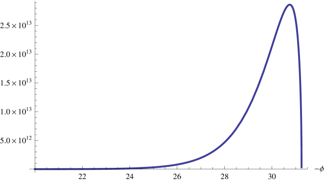
Figure 1: Effective equation solution for the expectation value of volume $\nu(\phi)$ is plotted with a $-\phi$ axis. The volume is exponentially increasing with $-\phi$ over a large range of values until it begins a sharp descent when the square-root term of Eqn. (58) approaches zero at $-\phi\approx 30.75$.

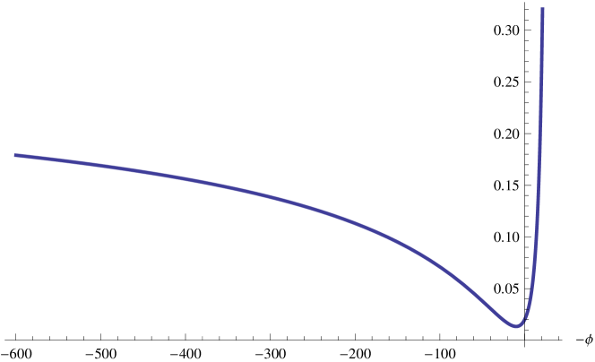
Figure 2: Relative fluctuation of volume $G^{\nu\nu}(\phi)/\nu(\phi)^{2}$ is plotted with a $-\phi$ axis. It is well behaved over a large range of values but does increase sharply at $-\phi>30.75$ and is increasingly larger for $-\phi<-20$ where $\nu(\phi)$ becomes small.

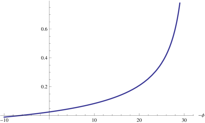
Figure 3: Relative covariance fluctuation of the volume and curvature expectation values $G^{b\nu}(\phi)/(b(\phi)\nu(\phi))$ is plotted with a $-\phi$ axis. It is reasonably well behaved over a large range of values, though it increases unboundedly at large $-\phi$, which is inconsistent with our semiclassical approximations in that region.

Let us then explore this system numerically for $H_{-1}$ positive, $\nu_{0}=10,b_{0}=1,G^{bb}_{0}=0.2,G^{\nu\nu}_{0}=2,G^{b\nu}_{0}=0.25$, noting that our initial values satisfy the uncertainty relation (where we set $\hbar=1$ for our numerics)

$$G^{\nu\nu}G^{bb}-(G^{b\nu})^{2}\geq\frac{\hbar^{2}}{4}.$$ (59)

Using our truncated equations of motion, Eqs. (50) – (54), we can easily verify that the uncertainty relation is preserved, that is

$$\frac{{\rm d}}{{\rm d}\phi}\left(G^{\nu\nu}G^{bb}-(G^{b\nu})^{2}\right)=0$$ (60)

and so will remain satisifed for all $\phi$. In Figure 1, we see that our values do indeed lead to a collapse at late negative time $\phi$ (plotted with $\phi$ increasingly negative to the right for convenience, as we will do with all of this section’s numerics). However, for this plot to be meaningful, we must verify the consistency of our assumptions within this region. In Figure 2 we see that the relative volume fluctuation $G^{\nu\nu}(\phi)/\nu^{2}(\phi)$ is well behaved for most of $\phi$, only increasing to the upper limits of our assumption of small relative fluctuations when $\nu(\phi)$ becomes exponentially small for $-\phi<-20$. In fact, from our analytic solutions given by Eqs. (56) and (58), we see that the relative volume fluctuations $G^{\nu\nu}/\nu^{2}$ asymptotically approaches a local maximum for $-\phi\rightarrow-\infty$:

$$\lim_{\phi\rightarrow\infty}\frac{G^{\nu\nu}(\phi)}{\nu^{2}(\phi)}=\frac{4C_{1}^{2}C_{2}}{(C_{1}^{2}+3C_{2})^{2}}=\frac{4b_{0}^{2}G^{bb}_{0}}{(b_{0}^{2}+3G^{bb}_{0})^{2}}$$ (61)

which is $0.3125$ for the numerical example used for our graphs (however, graphing the large $\phi$ regime numerically would require a very large number of integration steps). Near the turning point of $\nu$ at $-\phi>30$, the relative volume fluctuation begins to increase, quickly surpassing our assumption of small relative values. From Eqs. (55) we see that relative curvature fluctuations $G^{bb}(\phi)/b^{2}(\phi)$ will remain constant according to where we set them by our constants $b_{0}$ and $G^{bb}_{0}$.

In Figure 3 we see that the relative covariance $G^{b\nu}/(b(\phi)\nu(\phi))$ also surpasses our assumption of relatively small moments as it approaches the turning point of $\nu$, becoming unboundedly large as $\nu$ collapses at large $-\phi>30$. In addition, higher inverse powers of $b$ contributing to the Hamiltonian with generic factor ordering will become important near the potential recollapse. Thus, while we see collapse in Figure 1, it coincides with a breakdown of our assumptions in the regime where $b$ becomes exponentially small: a regime where higher inverse powers of curvature can become important, even when paired with inverse-volume terms. (We can also explore the opposite sign choice for $H_{-1}$ negative which is what our example from Subsection 4.1 had. In that case, the squareroot in $\nu(\phi)$ of Eq. (1) goes to zero as $\phi\rightarrow\infty$. However, rather than insinuating a recollapse, this is the regime where $\nu(\phi)\rightarrow 0$ and $b(\phi)$ gets exponentially large, indicating a singularity. Regardless of sign choice, in this regime we would require a higher-curvature expansion by positive powers of $b$ for holonomy (or other) corrections and quantum back-reaction before any physical meaning can be drawn from such analysis.)

6 Conclusion

This article discusses the influence of factor-ordering choices on effective equations in quantum cosmology, with possible modifications from loop quantization. As we have emphasized, the quantization of the Hamiltonian constraint is far from being unique even in the most reduced models. While deparameterized models may offer simple quantization choices, they are not the most general or natural ones. Quantum corrections and an analysis of semiclassical physics must therefore take these ambiguities into account.

We have implemented such an analysis to study the question of whether quantum effects in long-term semiclassical evolution could lead to significant departures from classical behavior, for instance a recollapse of spatially flat isotropic models. Since the model we analyzed allows a quantization free of quantum back-reaction, low-curvature effects could only come from factor-ordering corrections. We developed a suitable parameterization of factor-ordering ambiguities in effective equations, paying special attention to deparameterization choices. The generality of effective equations indeed allows us to draw conclusions, indicating that too-drastic effects do not occur. Our results therefore do not lead to concrete reasons for unexpected late-time effects in semiclassical (loop) quantum cosmology. But they provide strong caution against too-quick positive assurances of a straightforward classical limit based on the analysis of a few simple models and orderings.

In particular, it does not appear possible to have quantum corrections of the modified Friedmann equation independent of the energy density in this formulation. Thus, quantum collapse at low energy densities or large scales does not seem feasible by this mechanism given our corrections and assumptions. The only possibility, according to our analysis, would be to have inverse-triad corrections with a function $f(\nu)$ increasing more strongly than linearly, but this is not acceptable by the classical limit of the Hamiltonian constraint.

Furthermore, we explored the effects of factor ordering choices at first semiclassical order. A general tractable parameterization of quantization ambiguities in this regime surprisingly turns out to require a second expansion by the inverse Hubble parameter. Although the solutions to these effective equations hint at the possibility of a recollapse, the expansion by the inverse Hubble parameter breaks down before a recollapse could be reached. Interestingly, also some relative fluctuations grow too large to satisfy our approximations for all $\phi$ of interest. Extending such an analysis to higher quantum moments could be fruitful; for instance, unlimited semiclassical evolution may be possible within our expansion scheme if there are corrections to $b(\phi)$ such that it does not asymptotically approach zero, thus preventing factor ordering terms $1/b$ to approach infinity. For now, however, the semiclassical behavior of generic quantum cosmology remains incompletely understood.

References

- [1] M. Bojowald, Large scale effective theory for cosmological bounces, Phys. Rev. D 75 (2007) 081301(R), [gr-qc/0608100]
- [2] Y. Ding, Y. Ma, and J. Yang, Effective Scenario of Loop Quantum Cosmology, Phys. Rev. Lett. 102 (2009) 051301, [arXiv:0808.0990]
- [3] V. Taveras, Corrections to the Friedmann Equations from LQG for a Universe with a Free Scalar Field, Phys. Rev. D 78 (2008) 064072, [arXiv:0807.3325]
- [4] A. Ashtekar, M. Bojowald, and J. Lewandowski, Mathematical structure of loop quantum cosmology, Adv. Theor. Math. Phys. 7 (2003) 233–268, [gr-qc/0304074]
- [5] D. L. Wiltshire, An introduction to quantum cosmology, In B. Robson, N. Visvanathan, and W. S. Woolcock, editors, Cosmology: The Physics of the Universe, pages 473–531. World Scientific, Singapore, 1996, [gr-qc/0101003]
- [6] M. Bojowald, Loop Quantum Cosmology, Living Rev. Relativity 11 (2008) 4, [gr-qc/0601085], http://www.livingreviews.org/lrr-2008-4
- [7] M. Bojowald, Quantum Cosmology: A Fundamental Theory of the Universe, Springer, New York, 2011
- [8] C. Rovelli, Quantum Gravity, Cambridge University Press, Cambridge, UK, 2004
- [9] T. Thiemann, Introduction to Modern Canonical Quantum General Relativity, Cambridge University Press, Cambridge, UK, 2007, [gr-qc/0110034]
- [10] A. Ashtekar and J. Lewandowski, Background independent quantum gravity: A status report, Class. Quantum Grav. 21 (2004) R53–R152, [gr-qc/0404018]
- [11] C. Rovelli and L. Smolin, Loop Space Representation of Quantum General Relativity, Nucl. Phys. B 331 (1990) 80–152
- [12] M. Bojowald and H. A. Kastrup, Symmetry Reduction for Quantized Diffeomorphism Invariant Theories of Connections, Class. Quantum Grav. 17 (2000) 3009–3043, [hep-th/9907042]
- [13] M. Bojowald, Mathematical structure of loop quantum cosmology: Homogeneous models, [arXiv:1206.6088]
- [14] M. Bojowald, Degenerate Configurations, Singularities and the Non-Abelian Nature of Loop Quantum Gravity, Class. Quantum Grav. 23 (2006) 987–1008, [gr-qc/0508118]
- [15] M. Bojowald and A. Skirzewski, Quantum Gravity and Higher Curvature Actions, Int. J. Geom. Meth. Mod. Phys. 4 (2007) 25–52, [hep-th/0606232]
- [16] M. Bojowald, S. Brahma, and E. Nelson, Higher time derivatives in effective equations of canonical quantum systems, Phys. Rev. D 86 (2012) 105004, [arXiv:1208.1242]
- [17] K. Vandersloot, On the Hamiltonian Constraint of Loop Quantum Cosmology, Phys. Rev. D 71 (2005) 103506, [gr-qc/0502082]
- [18] P. Singh, Loop cosmological dynamics and dualities with Randall-Sundrum braneworlds, Phys. Rev. D 73 (2006) 063508, [gr-qc/0603043]
- [19] A. Ashtekar, T. Pawlowski, and P. Singh, Quantum Nature of the Big Bang: Improved dynamics, Phys. Rev. D 74 (2006) 084003, [gr-qc/0607039]
- [20] M. Bojowald, How quantum is the big bang?, Phys. Rev. Lett. 100 (2008) 221301, [arXiv:0805.1192]
- [21] M. Bojowald, Loop Quantum Cosmology IV: Discrete Time Evolution, Class. Quantum Grav. 18 (2001) 1071–1088, [gr-qc/0008053]
- [22] M. Bojowald, Isotropic Loop Quantum Cosmology, Class. Quantum Grav. 19 (2002) 2717–2741, [gr-qc/0202077]
- [23] M. Bojowald, The Semiclassical Limit of Loop Quantum Cosmology, Class. Quantum Grav. 18 (2001) L109–L116, [gr-qc/0105113]
- [24] J. Haro and E. Elizalde, Effective gravity formulation that avoids singularities in quantum FRW cosmologies, [arXiv:0901.2861]
- [25] R. Helling, Higher curvature counter terms cause the bounce in loop cosmology, [arXiv:0912.3011]
- [26] M. Bojowald and A. Skirzewski, Effective Equations of Motion for Quantum Systems, Rev. Math. Phys. 18 (2006) 713–745, [math-ph/0511043]
- [27] J. Yang, Y. Ding and Y. Ma, Alternative quantization of the Hamiltonian in loop quantum cosmology, Phys. Lett. B 682 (2009) 1–7, [arXiv:0904.4379]
- [28] L. Qin and Y. Ma, Coherent state functional integrals in quantum cosmology, Phys. Rev. D 85 (2012) 063515, [arXiv:1110.5480]
- [29] L. Qin and Y. Ma, Coherent state functional Integral in Loop Quantum Cosmology: Alternative Dynamics, Mod. Phys. Lett. A 27 (2012) 1250078, [arXiv:1206.1128]
- [30] M. Bojowald, Dynamical coherent states and physical solutions of quantum cosmological bounces, Phys. Rev. D 75 (2007) 123512, [gr-qc/0703144]
- [31] J. F. Barbero G., Real Ashtekar Variables for Lorentzian Signature Space-Times, Phys. Rev. D 51 (1995) 5507–5510, [gr-qc/9410014]
- [32] G. Immirzi, Real and Complex Connections for Canonical Gravity, Class. Quantum Grav. 14 (1997) L177–L181
- [33] M. Bojowald, Loop quantum cosmology and inhomogeneities, Gen. Rel. Grav. 38 (2006) 1771–1795, [gr-qc/0609034]
- [34] T. Thiemann, QSD V: Quantum Gravity as the Natural Regulator of Matter Quantum Field Theories, Class. Quantum Grav. 15 (1998) 1281–1314, [gr-qc/9705019]
- [35] M. Bojowald, Inverse Scale Factor in Isotropic Quantum Geometry, Phys. Rev. D 64 (2001) 084018, [gr-qc/0105067]
- [36] M. Bojowald and G. Calcagni, Inflationary observables in loop quantum cosmology, JCAP 1103 (2011) 032, [arXiv:1011.2779]
- [37] M. Bojowald, B. Sandhöfer, A. Skirzewski, and A. Tsobanjan, Effective constraints for quantum systems, Rev. Math. Phys. 21 (2009) 111–154, [arXiv:0804.3365]
- [38] M. Bojowald, D. Mulryne, W. Nelson, and R. Tavakol, The high-density regime of kinetic-dominated loop quantum cosmology, Phys. Rev. D 82 (2010) 124055, [arXiv:1004.3979]
- [39] M. Bojowald, D. Brizuela, H. H. Hernandez, M. J. Koop, and H. A. Morales-Técotl, High-order quantum back-reaction and quantum cosmology with a positive cosmological constant, Phys. Rev. D 84 (2011) 043514, [arXiv:1011.3022]
- [40] T. Thiemann, Quantum Spin Dynamics (QSD), Class. Quantum Grav. 15 (1998) 839–873, [gr-qc/9606089]
- [41] M. Bojowald, Quantization ambiguities in isotropic quantum geometry, Class. Quantum Grav. 19 (2002) 5113–5130, [gr-qc/0206053]
- [42] M. Bojowald, Loop Quantum Cosmology: Recent Progress, Pramana 63 (2004) 765–776, [gr-qc/0402053]
- [43] M. Bojowald and G. M. Paily, Deformed General Relativity and Effective Actions from Loop Quantum Gravity, Phys. Rev. D 86 (2012) 104018, [arXiv:1112.1899]
- [44] J. Mielczarek, Signature change in loop quantum cosmology, [arXiv:1207.4657]
- [45] M. Bojowald, Quantum nature of cosmological bounces, Gen. Rel. Grav. 40 (2008) 2659–2683, [arXiv:0801.4001]
- [46] X. Wu and Y. Ma, Effective Theories of Quantum Cosmology, [arXiv:1212.5874]
- [47] P. Malkiewicz, Reduced phase space approach to Kasner universe and the problem of time in quantum theory, Class. Quantum Grav. 29 (2012) 075008, [arXiv:1105.6030]
- [48] S. Alexander, M. Bojowald, A. Marciano, and D. Simpson, Electric time in quantum cosmology, Class. Quantum Grav. (2013) to appear, [arXiv:1212.2204]
- [49] M. Bojowald, P. A. Höhn, and A. Tsobanjan, An effective approach to the problem of time, Class. Quantum Grav. 28 (2011) 035006, [arXiv:1009.5953]
- [50] M. Bojowald, P. A. Höhn, and A. Tsobanjan, An effective approach to the problem of time: general features and examples, Phys. Rev. D 83 (2011) 125023, [arXiv:1011.3040]
- [51] P. A. Höhn, E. Kubalova, and A. Tsobanjan, Effective relational dynamics of a nonintegrable cosmological model, Phys. Rev. D 86 (2012) 065014, [arXiv:1111.5193]