Dipolar Bose-Einstein condensates in a $\mathcal{PT}\!$-symmetric double-well potential

Abstract

We investigate dipolar Bose-Einstein condensates in a complex external double-well potential that features a combined parity and time-reversal symmetry. On the basis of the Gross-Pitaevskii equation we study the effects of the long-ranged anisotropic dipole-dipole interaction on ground and excited states by the use of a time-dependent variational approach. We show that the property of a similar non-dipolar condensate to possess real energy eigenvalues in certain parameter ranges is preserved despite the inclusion of this nonlinear interaction. Furthermore, we present states that break the $\mathcal{PT}\leavevmode\nobreak\$symmetry and investigate the stability of the distinct stationary solutions. In our dynamical simulations we reveal a complex stabilization mechanism for $\mathcal{PT}\!$-symmetric, as well as for $\mathcal{PT}\!$-broken states which are, in principle, unstable with respect to small perturbations.

I Introduction

Open quantum systems and their effects, such as damping, dephasing, resonance phenomena and more, can be described by non-Hermitian Hamiltonians Moiseyev (2011). In particular, there are problems where the non-Hermitian quantum mechanics formalism is necessary, as e.g. in quantum field theory, or where it supports a simple description as in optics for a complex refraction index, or in cases where complex potentials are introduced Moiseyev (2011). Furthermore, it is sometimes quite advantageous to use non-Hermitian Hamiltonians although the problem could, in principle, be solved within the conventional Hermitian framework. One of the most important applications is the modeling of dissipation and influx by a complex potential. The formalism has been originally developed for the linear Schrödinger equation, however, it is applicable to the nonlinear Gross-Pitaevskii equation (GPE), as well. A widely-used procedure is the implementation of inelastic three-body losses in terms of an imaginary potential Köberle et al. (2012). Moreover, non-Hermitian forms of the GPE provide access to the decay of the condensates with the complex scaling approach Moiseyev and Cederbaum (2005); Schlagheck and Paul (2006), to transport phenomena Paul et al. (2007), and to the theoretical study of dissipative optical lattices Abdullaev et al. (2010); Bludov and Konotop (2010). An analytical continuation of the GPE made it possible to discover exceptional points (EPs) and study their properties Cartarius et al. (2008); Gutöhrlein et al. (2013).

One special class of non-Hermitian Hamiltonians are the $\mathcal{PT}\!$-symmetric ones. They commute with the $\mathcal{PT}\leavevmode\nobreak\$operator, which combines the action of parity and time reflection, i.e. $\left[\mathcal{PT},H\right]=0$. Bender and Boettcher Bender and Boettcher (1998); Bender et al. (1999) found that real eigenvalues are possible despite the non-Hermiticity of those Hamiltonians and in a certain parameter range completely real eigenvalue spectra can exist . Experimental observations of $\mathcal{PT}\leavevmode\nobreak\$symmetry have been achieved in optical systems Guo et al. (2009); Rüter et al. (2010); Regensburger et al. (2012), yet no $\mathcal{PT}\!$-symmetric genuine quantum system could be realized. In Refs. Cartarius and Wunner (2012); Dast et al. (2013a) it has been shown that Bose-Einstein condensates (BECs) in $\mathcal{PT}\!$-symmetric double-delta and double-well potentials, respectively, constitute such systems. Furthermore, in Refs. Dast et al. (2013a, b) the effect of the short-ranged contact interaction of the particles on the stationary states and on the dynamics has been investigated. There, good agreement with the results obtained by Graefe et al. Graefe et al. (2008, 2010) via a simple matrix model has been proven.

The experimental realization of atoms sustaining a large magnetic dipole moment e.g. ${}^{52}\mathrm{Cr}$ Griesmaier et al. (2005); Beaufils et al. (2008); T. Lahaye et al. (2009) and, more recently, ¹⁶⁴Dy Lu et al. (2010, 2011) and ${}^{168}\mathrm{Er}$ Aikawa et al. (2012) as well as the fast progress towards the creation of BECs of polar molecules Ni et al. (2008), which possess large electric dipole moments, opened the field of research for effects generated by the dipole-dipole interaction (DDI). It has been shown in LABEL:~Dast et al. (2013b) by mathematical arguments concerning the DDI that effects, typical for $\mathcal{PT}\!$-symmetric systems, are expected to be present in a dipolar $\mathcal{PT}\!$-symmetric system, as well. Considering not only the short-ranged contact, but also the long-ranged anisotropic DDI leads to interesting questions for $\mathcal{PT}\!$-symmetric systems: What is the impact of the DDI on the stationary states? In particular, real eigenvalues require $\mathcal{PT}\!$-symmetric wave functions, for which the effects of gain and loss modeled by imaginary potentials are balanced. This relation between true stationary states with real eigenvalues and the symmetry of the wave function also holds in the nonlinear GPE Cartarius and Wunner (2012); Dast et al. (2013a, b); Graefe et al. (2008, 2010) and is even more important since a wave function breaking the $\mathcal{PT}\leavevmode\nobreak\$symmetry of the linear potential may even destroy that of the total nonlinear Hamiltonian. It is well known that the anisotropic DDI can lead even to structured ground states not possessing the potential’s symmetry. In combination with gain and loss effects this opens the door for new cases of $\mathcal{PT}\leavevmode\nobreak\$symmetry breaking. The scenario for BECs in a $\mathcal{PT}\!$-symmetric potential that feature solely short-ranged interactions can be described by a simple matrix model, as shown by Graefe et al. Graefe et al. (2008, 2010) for a two-mode Bose-Hubbard system. These results are in agreement with a mean-field description within the GPE Dast et al. (2013b). We expect new effects to arise from the DDI and particularly from its long-range nature that is not included in the matrix model. Furthermore, dipolar condensates often feature novel dynamical properties and provide effects such as long-ranged Josephson oscillations Asad-uz-Zaman and Blume (2009); Xiong et al. (2009) or pattern formation Nath et al. (2009) and it is therefore interesting to explore the time evolution of dipolar condensates in a $\mathcal{PT}\!$-symmetric potential.

In this work we combine the ingredients of the long-ranged DDI with the $\mathcal{PT}\leavevmode\nobreak\$symmetry of an external potential. Thereby we consider a dipolar condensate in a $\mathcal{PT}\!$-symmetric double-well potential and extend the work presented in LABEL:~Dast et al. (2013a) to dipolar BECs. Our analysis is based on the time-dependent extended Gross-Pitaevskii equation

$$\mathrm{i}\frac{\mathrm{d}}{\mathrm{d}t}\Psi\left(\bm{r},t\right)=\left[-\frac{1}{2}\Delta+V_{\mathrm{ext}}+V_{\mathrm{c}}+V_{\mathrm{dd}}\right]\Psi\left(\bm{r},t\right)\,,$$ (1)

where $V_{\mathrm{ext}}$, $V_{\mathrm{c}}$, and $V_{\mathrm{dd}}$ denote the external, short-ranged contact and long-ranged dipole-dipole interaction potential, respectively. In Eq. (1) and for the potentials below, we choose the units of energy $E$, time $t$, and length $\bm{r}$ such that $[E]=\hbar^{2}/(ml^{2})$, $[t]=ml^{2}/\hbar$, and $[\bm{r}]=l$, where $l$ is the distance between the centers of the two wells (cf. Fig. 1).

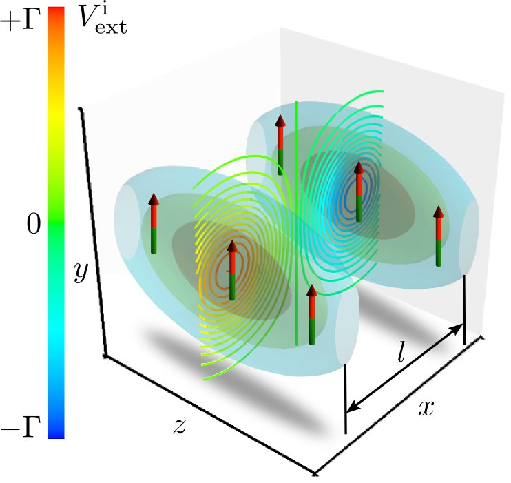
Figure 1: (Color online) Visualization of the $\mathcal{PT}\!$-symmetric double-well potential in the repulsive configuration. The arrows indicate the direction of the dipoles. Isosurfaces show the shape of the real part $V_{\mathrm{ext}}^{\mathrm{r}}$ of the external potential, where $l$ is the inter-well spacing as given in the text. The contour lines show a slice cut through the center of the imaginary part $V_{\mathrm{ext}}^{\mathrm{i}}$ of the external potential, with the corresponding colorbars on the left.

The external potential is modeled in our calculations by

$$V_{\mathrm{ext}}(\bm{r}) =-\left(V_{0}-\mathrm{i}\Gamma\right)g^{+}-\left(V_{0}+\mathrm{i}\Gamma\right)g^{-}\,,$$ (2)

$$\text{with}\quad g^{\pm} =\exp\left(-\frac{(x\pm l/2)^{2}}{2L_{x}^{2}}-\frac{y^{2}}{2L_{y}^{2}}-\frac{z^{2}}{2L_{z}^{2}}\right)\,,$$ (3)

where $V_{0}$ is the depth of the real double-well potential and $\Gamma$ is the strength of the gain and loss terms. We choose the identical parameters as given in Refs. Peter et al. (2012); Fortanier et al. (2013) for a similar triple-well system $V_{0}=80$, $L_{x}=L_{z}=1/4$, and $L_{y}=2$, as these have a reasonable magnitude for a possible corresponding experiment. The contact interaction potential $V_{\mathrm{c}}$ reads

$$V_{\mathrm{c}}=4\pi Na\left|\Psi\left(\bm{r},t\right)\right|^{2}\,,$$ (4)

with the scattering length $a$ and the number of particles $N$. The DDI potential is given by

$$V_{\mathrm{dd}}=3Na_{\mathrm{dd}}\int\mathrm{d}^{3}r^{\prime}\frac{1-3\cos^{2}\theta}{\left|\bm{r}-\bm{r}^{\prime}\right|^{3}}\left|\Psi\left(\bm{r}^{\prime},t\right)\right|^{2}\,,$$ (5)

where $a_{\mathrm{dd}}$ is the dipole strength and $\theta$ is the angle between the vector $\bm{r}-\bm{r}^{\prime}$ and the direction of the dipole alignment. The dipolar interaction breaks the symmetry and provides two possible configurations, namely the repulsive configuration, shown in Fig. 1, where the dipoles are aligned in $y$-direction and the attractive configuration, where the dipoles are aligned in $x$-direction. We will only discuss the repulsive configuration, yet we have also performed calculations in the attractive configuration, but found a qualitatively similar behavior.

II Method

Our method is based on the time-dependent variational principle (TDVP) with the variational ansatz consisting of a linear superposition of two Gaussian wave packets (GWPs), $\Psi=g^{1}+g^{2}$. Details of the method can be found in Eichler et al. (2012), where the same method has been used to describe the collision of quasi-2$d$ anisotropic solitons and in Fortanier et al. (2013), where dipolar BECs in triple-well potentials have been investigated. Yet, we will recapitulate the major steps for the reader’s convenience here. Each of the GWPs has the form

$$g^{k}=\mathrm{e}^{-\left(\left(\bm{x}-\bm{q}^{k}\right)^{T}A^{k}\left(\bm{x}-\bm{q}^{k}\right)-\mathrm{i}\left(\bm{p}^{k}\right)^{T}\left(\bm{x}-\bm{q}^{k}\right)+\gamma^{k}\right)}\,,$$ (6)

where $k=1,2$; the symbol $T$ denotes the transposition and where in general the time-dependent parameters $A^{k}$ are $3\times 3$ complex diagonal matrices, $\bm{p}^{k}$ and $\bm{q}^{k}$ are real 3$d$ vectors, and $\gamma^{k}$ are complex numbers. We assume that the $y$-direction (the direction of the dipole alignment) has a strong confinement due to the external trap and thus ignore translations and rotations in this direction i.e. $q_{y}^{k}\equiv 0$, $A^{k}_{xy}=A^{k}_{yz}\equiv 0$. However, for the other directions we apply no further restrictions, particularly with respect to position and movement of the GWPs in the $x$-direction. It is reasonable to start with one GWP placed at the center of each well.

To determine the time development of the variational parameters we make use of the TDVP in the formulation of McLachlan McLachlan (1964)

$$I=\left|\left|\mathrm{i}\phi-H\Psi(t)\right|\right|^{2}\stackrel{{\scriptstyle!}}{{=}}\min\,,$$ (7)

where $\phi$ is varied and set $\phi\equiv\dot{\Psi}$ afterwards. We then apply the ansatz

$$\Psi =g^{1}+g^{2}$$ (8)

for the variational wave function, which yields the equations of motion (EOM) for the variational parameters

$$\dot{\bm{z}}=\bm{f}\left(\bm{z}(t)\right)=\bm{f}\left(A^{k}(t),\bm{q}^{k}(t),\bm{p}^{k}(t),\gamma^{k}(t)\right)\,,$$ (9)

with $\bm{z}=(\bm{z}^{1},\bm{z}^{2})$ and $k=1,2$.

The stationary states of the GPE are the fixed points of Eq. (9) and can be determined by a nonlinear root search (e.g. Newton-Raphson). An alternative to find the real ground state is the application of imaginary time evolution (ITE) to the EOM. However, the ITE does not always converge to the ground state Fortanier et al. (2013); Menotti et al. (2007). To evolve the EOM in imaginary time as well as in real time, a standard algorithm like Runge-Kutta can be used.

We investigate the linear stability of the fixed points by the calculation of the eigenvalues $\Lambda=\Lambda^{\mathrm{r}}+\mathrm{i}\Lambda^{\mathrm{i}}$ of the Jacobian

$$J=\frac{\partial\left(\mathrm{Re}\,\dot{A}^{k},\mathrm{Im}\,\dot{A}^{k},\dot{\bm{q}}^{k},\dot{\bm{p}}^{k},\mathrm{Re}\,\dot{\gamma}^{k},\mathrm{Im}\,\dot{\gamma}^{k}\right)}{\partial\left(\mathrm{Re}\,A^{j},\mathrm{Im}\,A^{j},{\bm{q}^{j}},{\bm{p}^{j}},\mathrm{Re}\,{\gamma^{j}},\mathrm{Im}\,{\gamma^{j}}\right)}\,,$$ (10)

with $k,j=1,2$. The eigenvalues $\Lambda$ appear in pairs of opposite sign and correspond to excitations described by the Bogoliubov-de Gennes equations Kreibich et al. (2012, 2013a); Rau et al. (2010a, b). If all real parts $\Lambda^{\mathrm{r}}$ vanish, the fixed point is stable, otherwise it is unstable.

The parameter space is essentially spanned by the three parameters $Na_{\mathrm{dd}}$, $Na$, and $\Gamma$, whereas the particle number $N$ is no independent quantity due to the scaling properties of the GPE. For reasons of clearness we keep the dipole strength constant at $Na_{\mathrm{dd}}=0.3$. In order to obtain the states over the range of interest for the remaining two parameters it is reasonable in the numerical computation to start at $Na=0$ and $\Gamma=0$, where the algorithm is most stable and ground states are accessible by an imaginary-time evolution. Afterwards we advance with the result as initial guess for the nonlinear root search. However, it turned out that this method does not guarantee to find the correct states for several reasons. The number of existing states is not constant and, as we will see later on, states emerge and vanish in bifurcations. Furthermore, crossings of states appear. Then, an extrapolation of the previously obtained variational parameters may lead to a unfortunate choice of initial parameters, and only a subtle algorithm is capable to advance them. We use any of the following strategies to obtain results in such cases: we circumvent the crossings by advancing the other parameter, we perform forward-jumps and proceed to calculate backwards, or we perform an extrapolation of the variational parameters close to a bifurcation point depending on the bifurcation type (e.g. square root behavior of a tangent bifurcation).

III Results

The presence of the dipolar interaction strongly influences the results for the stationary states in all kinds of real external potentials. We therefore briefly summarize the picture that one obtains for the case $\Gamma=0$. A BEC in a real double-well potential, with no gain or loss present, exhibits spontaneous symmetry breaking, also known as macroscopic quantum self-trapping, above a critical value of the scattering length. This effect breaks the symmetry of the external trap and occurs both in a system with dipolar and pure contact interactions Xiong et al. (2009); Raghavan et al. (1999); Theocharis et al. (2006). To distinguish between the effects originating from short-ranged and long-ranged interactions in a real external potential it is more appropriate to choose a triple-well system Fortanier et al. (2013); Peter et al. (2012); Zhang and Xue (2012); Lahaye et al. (2010). However, regarding the stationary states, dipolar effects can be identified as we will show in Sec. III.2.

III.1 Stationary states of non-dipolar BECs

It turns out that the spectra we obtain for the dipolar condensate in the $\mathcal{PT}\!$-symmetric double well involve more states than in the non-dipolar case. To understand the influence of the DDI we want to relate our findings to the simpler case of a BEC which only possesses short-ranged interactions. In LABEL:~Dast et al. (2013a) results have been presented for the non-dipolar system, yet within a different unit system and with a different specific form of the external potential. For the convenience of the reader we here qualitatively confirm these results for the potential (2) with the units given above and subsequently compare the findings in the dipolar system with them.

In Fig. 2 real and imaginary parts of the mean-field energy for the non-dipolar case are shown. For vanishing nonlinearity $Na=0$ two $\mathcal{PT}\!$-symmetric states with purely real eigenvalues exist from $\Gamma=0$ up to a critical value of the gain-loss parameter $\Gamma$. At this point, labeled $E$ in Fig. 2, these states vanish in a bifurcation and two $\mathcal{PT}\!$-broken states with complex conjugate energies emerge. For these states only $E^{\mathrm{i}}_{\mathrm{mf}}\geq 0$ is shown. As soon as the nonlinearity is present the tangent bifurcation at point $E$ splits up into a tangent bifurcation $T$, where the $\mathcal{PT}\!$-symmetric states vanish, and a pitchfork bifurcation $P$, where the $\mathcal{PT}\!$-broken states emerge. Note that although being solutions of the time-independent GPE, the $\mathcal{PT}\!$-broken solutions are no true stationary solutions for $\Gamma\neq 0$ due to the imaginary part in their energy eigenvalue. It has been shown in Refs. Heiss et al. (2013); Dast et al. (2013b) that the bifurcation points are exceptional points (EPs) of order 2 and 3. The singular point $E$ has some unique properties as shown in LABEL:~Dast et al. (2013b). There, an analytic continuation of the GPE has been performed. Due to the analytic continuation the number of states does no longer change at the bifurcation points $P$ and $T$. Two analytically continued states appear in addition to those shown in Fig. 2 for $\Gamma$ values below $P$. Similarly two additional analytically continued states are found for $\Gamma$ values above $T$. The extended states always exactly emerge in the bifurcation points, i.e. in the whole range of $\Gamma$ always four eigenstates are present in the shown energy range. In principle, excited states with much higher energies $E_{\mathrm{mf}}^{\mathrm{r}}$ could be found in the region $V_{0}<E_{\mathrm{mf}}^{\mathrm{r}}<0$, yet these states are energetically separated far enough as to influence the states investigated here. This argument can be applied to the dipolar system as well. In the limit $Na\rightarrow 0$ the points $P$ and $T$ merge and it can be shown that structures of a fourth-order EP are revealed. However, these structures are only observable as long as $Na\neq 0$. For $Na=0$ the analytic continuation of the GPE splits into two uncoupled parts that are equivalent to the non-extended GPE. Thus, only two identical spectra on top of each other with two identical second-order EPs at the only remaining bifurcation $E$ are observed.

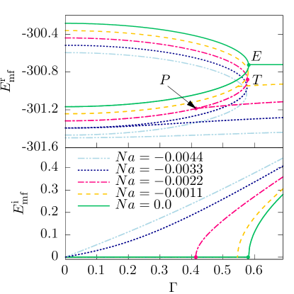
Figure 2: (Color online) Mean-field energy as a function of the gain-loss parameter $\Gamma$ at different values of the nonlinearity $Na$ for the non-dipolar case. The upper panel shows the real and the lower one the imaginary part. For $Na=-0.0022$ the tangent bifurcation is marked by a dot labeled $T$ and the pitchfork bifurcation by a dot labeled $P$. For $Na=0$ both bifurcations merge in the singular point $E$. $E_{\mathrm{mf}}$ and $\Gamma$ are given in the units introduced in Sec. I.

III.2 Stationary states of dipolar BECs

We will now include the dipolar interaction and investigate the system with the results of the non-dipolar case in mind. Although we performed calculations for a wide range of the parameters $Na$ and $\Gamma$ we will concentrate on a domain found to express interesting phenomena. Still, keep in mind that the following effects and characteristics can be present in different parameter regions for a different dipole strength $Na_{\mathrm{dd}}$.

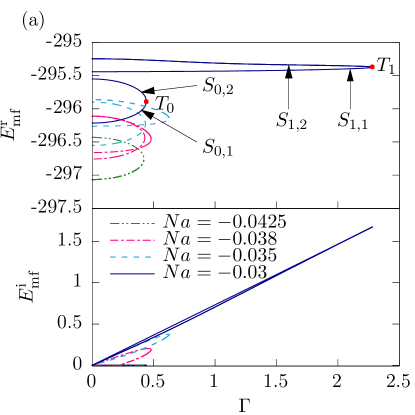
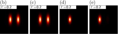
Figure 3: (Color online) (a) Mean-field energy of the stationary states in the repulsive configuration as a function of the gain-loss parameter $\Gamma$ for different values of $Na$. The upper panel shows the real and the lower one the imaginary part. The dipole strength is set to $Na_{\mathrm{dd}}=0.3$. For $Na=-0.03$ the arrows in (a) point at the lines of the states for which in (b) $S_{0,1}$, (c) $S_{0,2}$, (d) $S_{1,1}$, and (e) $S_{1,2}$ the absorption images are shown at $\Gamma=0.2$. The field of view is $1\times 1$ in the units given in the text. In (a) the two tangent bifurcations $T_{0}$ and $T_{1}$ are labeled with red dots.

In Fig. 3 results for $Na_{\mathrm{dd}}=0.3$ and several values of the scattering length $Na$ are given. We show the mean-field energy as a function of the gain-loss parameter $\Gamma$. For $Na=-0.03$ (solid blue line) at $\Gamma=0$ four different states are present. This denotes the situation of a real double-well potential and it is a remarkable result that the number of states is larger in the dipolar system than in the non-dipolar one for the corresponding situation, as shown in Fig. 2 for $Na=-0.0044$ (double-dotted dashed light-blue line) at $\Gamma=0$. Although this might stimulate attempts to gain a more complete picture for the stationary states of non-dipolar and dipolar BEC in a real double-well potential, we will concentrate on the investigation of the effects introduced by gain and loss here. The two states with the higher mean-field energy $S_{1,1}$ and $S_{1,2}$ break the $\mathcal{PT}\leavevmode\nobreak\$symmetry of the external potential as can be seen in Figs. 3(d) and (e). This leads to a finite imaginary part of the mean-field energy for $\Gamma\neq 0$. By the application of the $\mathcal{PT}\leavevmode\nobreak\$operator to these $\mathcal{PT}\!$-broken states $S_{1,\alpha}$; $\alpha=1,2$ two new states $S_{1,\alpha}^{\prime}$ which have complex conjugate $E_{\mathrm{mf}}$ can be generated. These new states $S_{1,\alpha}^{\prime}$ are also solutions of the time-independent GPE. However, we omit the states $S_{1,\alpha}^{\prime}$ in Fig. 3(a) and in the following discussion as the analysis of these states is the same as for the states $S_{1,\alpha}$. Note though that the dynamical behavior is different. The lower states $S_{0,1}$ and $S_{0,2}$ preserve the $\mathcal{PT}\leavevmode\nobreak\$symmetry and thus yield real $E_{\mathrm{mf}}$. Both pairs of states $S_{0,\alpha}$ and $S_{1,\alpha}$ disappear in two separate tangent bifurcations $T_{0}$ and $T_{1}$, respectively. Altogether six different states are present in the energy range of Fig. 2: Two $\mathcal{PT}\!$-symmetric states, and two pairs of $\mathcal{PT}\!$-broken states.

Decreasing the scattering length $Na$ causes $E_{\mathrm{mf}}^{\mathrm{r}}$ of the $\mathcal{PT}\!$-broken states to become smaller and approach the values of the $\mathcal{PT}\!$-symmetric states. In this process the mean-field energy of the state $S_{1,1}$ crosses both of the $\mathcal{PT}\!$-symmetric states $S_{0,\alpha}$ (see e.g. dashed blue curve for $Na=-0.035$ in Fig. 3(a)), yet the crossing point is no exceptional point, i.e. the wave functions are diverse. A further decrease of $Na$ has an effect similar to that observed in Refs. Dast et al. (2013a, b). From here on we include Fig. 4 for a detailed discussion. The state $S_{1,2}$ separates in a pitchfork bifurcation from the $\mathcal{PT}\!$-symmetric state $S_{0,2}$ (see red dashed-dotted line for $Na=-0.038$ in Fig. 4).

Figure 4: (Color online) Mean-field energy as a function of the gain-loss parameter $\Gamma$, where the upper panel shows the real and the lower one the imaginary part. The dipole strength is set to $Na_{\mathrm{dd}}=0.3$. The points $P$ and $P^{\prime}$ denote pitchfork bifurcations for different values of the scattering length. At the point $E$ the pitchfork bifurcation has merged with the tangent bifurcation $T_{0}$ (see Fig. 3) of the $\mathcal{PT}\!$-symmetric states. Note that for $Na=-0.0415$ the $\mathcal{PT}\!$-broken state for values of $\Gamma<P^{\prime}$ has almost the same real part of the energy as the $\mathcal{PT}\!$-symmetric one and lies on top of that in the upper panel.

The pitchfork bifurcation is labeled $P$ in Fig. 4, whereas the tangent bifurcations of the $S_{0,\alpha}$ and $S_{1,\alpha}$ states are denoted $T_{0}$ and $T_{1}$, respectively, in Fig. 3. For the scattering length $Na\approx-0.03985$ (solid green line in Fig. 4) the tangent bifurcation $T_{0}$ of the $\mathcal{PT}\!$-symmetric states and the pitchfork bifurcation $P$ merge in one point, marked with a green dot, labeled $E$ in Fig. 4(a). This behavior in a variation of the scattering length $Na$ is therefore analogous to that in the non-dipolar case. Yet, here the $\mathcal{PT}\!$-broken state vanishes for larger $\Gamma$ in an additional tangent bifurcation $T_{1}$. It is a remarkable fact that here the point $E$ appears at nontrivial parameters and particularly for a finite nonlinearity and we will revisit this point in the outlook. At $E$ the energy eigenvalues obviously become real and the wave function preserves the $\mathcal{PT}\leavevmode\nobreak\$symmetry. Note that the tangent bifurcation $T_{1}$ has not merged with this point and remains separate at a slightly higher value of $\Gamma$.

Decreasing the scattering length further leads $P$ to move down the other $\mathcal{PT}\!$-symmetric state $S_{0,1}$, see e.g. the dashed yellow line for $Na=-0.0415$ in the lower panel of Fig. 4. There, the tangent bifurcation $T_{1}$ has already merged with the pitchfork bifurcation so that the state $S_{1,1}$ has disappeared and the state $S_{1,2}$ (see Fig. 3) is the only remaining $\mathcal{PT}\!$-broken state. If the scattering length is tuned even lower, $P$ is shifted to smaller values of $\Gamma$ until the remaining $\mathcal{PT}\!$-broken state eventually disappears and only $\mathcal{PT}\!$-symmetric states are left (see dashed-double-dotted green line for $Na=-0.0425$ in Fig. 3). If we decrease $Na$ from there on, both $\mathcal{PT}\!$-symmetric solutions would disappear as well. This behavior is well-known for a condensate in a real double-well potential Milburn et al. (1997).

III.3 Stability and dynamics

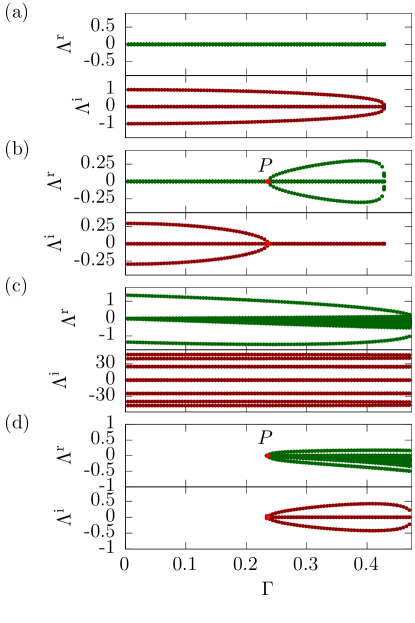
Figure 5: (Color online) Eigenvalues $\Lambda=\Lambda^{\mathrm{r}}+\mathrm{i}\Lambda^{\mathrm{i}}$ of the Jacobian (10) as functions of the gain-loss parameter $\Gamma$ with $Na=-0.038$, and $Na_{\mathrm{dd}}=0.3$. Figs. (a)–(d) show the states $S_{0,1}$, $S_{0,2}$, $S_{1,1}$, and $S_{1,2}$, respectively. In (a) all eigenvalues are imaginary with vanishing real parts implying stable fixed points. The upper state, shown in (b) is stable up to the pitchfork bifurcation $P$. The $\mathcal{PT}\!$-broken states $S_{1,\alpha}$; $\alpha=1,2$ shown in (c) and (d) are unstable in the whole range of $\Gamma$. In (d) the pitchfork bifurcation $P$ can be seen, where for values of $\Gamma<\Gamma_{P}$ only the state $S_{0,2}$ shown in (b) survives.

The linear stability of the stationary points is investigated by the use of the method presented in Sec. II. The vanishing real parts of all stability eigenvalues of the Jacobian (10) correspond to stable fixed points. In Fig. 5 the stability eigenvalues for $Na=-0.038$ (red dashed-dotted line in Fig. 4) are shown for all four states. The discussion of the states obtained by the application of the $\mathcal{PT}\!$-operator is analogous to the one of the states $S_{1,\alpha}$, except for the fact that in one case the norm is increasing and for the other case decreasing for small periods in time. The lowest-lying state $S_{0,1}$ is stable in the whole range of $\Gamma$ as it is not involved in any pitchfork bifurcation with a $\mathcal{PT}\!$-breaking state. This is different for the state $S_{0,2}$ (see Fig. 5(b)) which looses its stability around the pitchfork bifurcation at $\Gamma_{P}\approx 0.24$. The $\mathcal{PT}\!$-broken states shown in Figs. 5(c),(d) are unstable in the whole range, where they exist, as expected due to the complex energy eigenvalues.

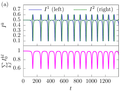
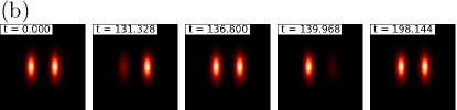
Figure 6: (Color online) Real-time evolution of the state $S_{0,2}$ for $Na_{\mathrm{dd}}=0.3$, $Na=-0.038$, and $\Gamma=0.2$. No additional perturbances other than numerical fluctuations have been added to the initial state. (a) The upper panel shows the populations $I^{k}=\langle g^{k}|g^{k}\rangle$, $k=1,2$ of the left and the right well. The lower panel shows the overall norm of the wave function. In (b) absorption images during the first oscillation are plotted with the parameters given in Fig. 3. It can be seen that during the oscillation the wave function takes the shape of the different $\mathcal{PT}\!$-broken states.

The real-time evolution of the stable state $S_{0,1}$ provides no further insight as all parameters stay constant. Yet, the corresponding evolution of the state $S_{0,2}$ reveals some very interesting effects. In Fig. 6 the real-time evolution of this $\mathcal{PT}\!$-symmetric state with a higher mean-field energy than $S_{0,1}$ is shown. At first the state remains approximately constant. Then a nonlinear oscillation between the wells sets in. The shape of the wave function, which is illustrated by the absorption images in Fig. 6(b), passes through states similar to the states shown in Figs. 3(b)–(e). This behavior can be interpreted in the following way. As $\Gamma<\Gamma_{P}$ the $\mathcal{PT}\!$-broken state has not separated from the state $S_{0,2}$ and the linear stability analysis declares the initial state stable. Yet, in this complex system, where amongst others the loss of norm conservation influences the dynamics, it is not sufficient to monitor the eigenvalues of the linearized problem, but an investigation of the full dynamics is required.

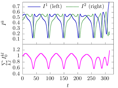
Figure 7: (Color online) Real-time evolution of the state $S_{1,2}$ for $Na_{\mathrm{dd}}=0.3$ and $Na=-0.038$. In contrast to Fig. 6, here $\Gamma=0.25$ is slightly above the value $\Gamma_{P}$ of the pitchfork bifurcation (see Fig. 5(b)), i.e. in the unstable regime. Yet, the nonlinear coupling dynamically stabilizes the state for several oscillations until the condensates finally collapses.

Interestingly, not only the amplitude shows that the oscillations observed in Fig. 6 cannot be classified as small. This is already observable in comparison with the smallest finite eigenvalue $\left|\Lambda^{\mathrm{i}}\left(\Gamma=0.2\right)\right|_{\mathrm{min}}\approx 1$ as the corresponding time scale would be one order of magnitude smaller than the time scale of the oscillations in Fig. 6. This confirms the fact that a strong nonlinear coupling between the $\mathcal{PT}\!$-symmetric and the $\mathcal{PT}\!$-broken states takes place. The strong coupling can already be seen by a close look e.g. at the pitchfork bifurcation $P$. There is a small gap between the values of $\Gamma_{P}$ obtained from the energies and the stability eigenvalues, which has been shown to originate from the nonlinearity in LABEL:~Löhle et al. (2014). The importance of the influences of both the loss of norm conservation and nonlinearity is impressively demonstrated in Fig. 7, where these prevent the collapse of the condensate by a dynamical stabilization mechanism for several oscillations. This is similar to the behavior of the non-dipolar case described in LABEL:~Haag et al. (2014) by a projection on the Bloch sphere, yet, this projection is not possible in the dipolar system. More drastically, we found cases, where a state that is unstable with respect to small perturbations, is dynamically stabilized completely, regarding the collapse. The dynamical behavior in such cases is similar to the nonlinear oscillations shown in Fig. 6. The larger the energetic distance between the states is, the smaller the coupling gets. A further increase of the gain-loss parameter suppresses the stabilization mechanism and for $\Gamma=0.4$ the local collapse is induced already by small perturbations of the stationary state.

IV Conclusion

We have shown that dipolar BECs in a $\mathcal{PT}\!$-symmetric double-well potential feature real stationary solutions in parts of the parameter space. Additionally, $\mathcal{PT}\!$-broken states are present, and in a distinct range of the scattering length $Na$ one more pair of states is present in the corresponding energy range than in the similar non-dipolar system Dast et al. (2013a). The pair of states vanishes in a tangent bifurcation together with the $\mathcal{PT}\!$-broken states observed also in Dast et al. (2013a). Furthermore, in the dipolar system a point is found, where the pitchfork bifurcation of the $\mathcal{PT}\!$-broken states merges with the tangent bifurcation of the $\mathcal{PT}\!$-symmetric ones. This singular point that has been shown in LABEL:~Dast et al. (2013b) to be related to an exceptional point of order 4 is found for a nontrivial value $Na\neq 0$ of the nonlinearity.

We found a strong influence of the nonlinearity on the dynamics of the system. Often a linear stability analysis is not sufficient to describe condensate wave functions close to stationary states. A nonlinear coupling is capable of stabilizing states predicted to be unstable by the linear stability eigenvalues or destabilizing states which are supposed to be stable.

From the fact that we found similar results for the attractive configuration one might ask the question if only the long-range nature of the DDI causes the qualitative picture. Then, such results should be observable e.g. with an isotropic long-range interaction as the $1/r$-interaction O’Dell et al. (2000). Furthermore, an appropriate matrix model has to be developed to describe the additional states and bifurcations. For a deeper understanding of the effects of the DDI the system should be extended to a $\mathcal{PT}\!$-symmetric triple-well potential, where it is easier to distinguish between on-site and long-ranged effects. In the investigation of the singular point $E$ in Fig. 4 an analytic continuation and encircling the point in the complex plane could reveal the properties of this interesting feature. In particular, the encircling will state clearly whether or not a true EP4 has been found.

The non-dipolar system of Refs. Dast et al. (2013a, b) can be regarded as a subsystem of a generic Hermitian system – in that case, e.g. a four-well system Kreibich et al. (2013b). Thereby, the outer wells serve as reservoirs of particles and constitute gain and loss, proposing an experimental realization. However, with the DDI the reservoirs are coupled to the inner wells by the long-ranged DDI and thus the realization of a $\mathcal{PT}\!$-symmetric dipolar system requires a different approach. Yet, this would be an interesting topic to investigate as the correspondence to a larger system might allow for the drawing of conclusions to the answers concerning the mechanisms in large dipolar systems.

References

- Moiseyev (2011) N. Moiseyev, Non-Hermitian quantum mechanics (Cambridge University Press, Cambridge, 2011).
- Köberle et al. (2012) P. Köberle, D. Zajec, G. Wunner, and B. A. Malomed, Phys. Rev. A 85, 023630 (2012).
- Moiseyev and Cederbaum (2005) N. Moiseyev and L. S. Cederbaum, Phys. Rev. A 72, 033605 (2005).
- Schlagheck and Paul (2006) P. Schlagheck and T. Paul, Phys. Rev. A 73, 023619 (2006).
- Paul et al. (2007) T. Paul, M. Hartung, K. Richter, and P. Schlagheck, Phys. Rev. A 76, 063605 (2007).
- Abdullaev et al. (2010) F. K. Abdullaev, V. V. Konotop, M. Salerno, and A. V. Yulin, Phys. Rev. E 82, 056606 (2010).
- Bludov and Konotop (2010) Y. V. Bludov and V. V. Konotop, Phys. Rev. A 81, 013625 (2010).
- Cartarius et al. (2008) H. Cartarius, J. Main, and G. Wunner, Phys. Rev. A 77, 013618 (2008).
- Gutöhrlein et al. (2013) R. Gutöhrlein, J. Main, H. Cartarius, and G. Wunner, J. Phys. A 46, 305001 (2013).
- Bender and Boettcher (1998) C. M. Bender and S. Boettcher, Phys. Rev. Lett. 80, 5243 (1998).
- Bender et al. (1999) C. M. Bender, S. Boettcher, and P. N. Meisinger, J. Math. Phys. 40, 2201 (1999).
- Guo et al. (2009) A. Guo, G. J. Salamo, D. Duchesne, R. Morandotti, M. Volatier-Ravat, V. Aimez, G. A. Siviloglou, and D. N. Christodoulides, Phys. Rev. Lett. 103, 093902 (2009).
- Rüter et al. (2010) C. E. Rüter, K. G. Makris, R. El-Ganainy, D. N. Christodoulides, M. Segev, and D. Kip, Nat. Phys. 6, 192 (2010).
- Regensburger et al. (2012) A. Regensburger, C. Bersch, M.-A. Miri, G. Onishchukov, D. N. Christodoulides, and U. Peschel, Nature 488, 167 (2012).
- Cartarius and Wunner (2012) H. Cartarius and G. Wunner, Phys. Rev. A 86, 013612 (2012).
- Dast et al. (2013a) D. Dast, D. Haag, H. Cartarius, G. Wunner, R. Eichler, and J. Main, Fortschritte der Physik 61, 124 (2013a).
- Dast et al. (2013b) D. Dast, D. Haag, H. Cartarius, J. Main, and G. Wunner, J. Phys. A 46, 375301 (2013b).
- Graefe et al. (2008) E. M. Graefe, U. Günther, H. J. Korsch, and A. E. Niederle, J. Phys. A 41, 255206 (2008).
- Graefe et al. (2010) E.-M. Graefe, H. J. Korsch, and A. E. Niederle, Phys. Rev. A 82, 013629 (2010).
- Griesmaier et al. (2005) A. Griesmaier, J. Werner, S. Hensler, J. Stuhler, and T. Pfau, Phys. Rev. Lett. 94, 160401 (2005).
- Beaufils et al. (2008) Q. Beaufils, R. Chicireanu, T. Zanon, B. Laburthe-Tolra, E. Maréchal, L. Vernac, J.-C. Keller, and O. Gorceix, Phys. Rev. A 77, 061601(R) (2008).
- T. Lahaye et al. (2009) T. Lahaye, C. Menotti, L. Santos, M. Lewenstein, and T. Pfau, Rep. Prog. Phys. 72, 126401 (2009).
- Lu et al. (2010) M. Lu, S. H. Youn, and B. L. Lev, Phys. Rev. Lett. 104, 063001 (2010).
- Lu et al. (2011) M. Lu, N. Q. Burdick, S. H. Youn, and B. L. Lev, Phys. Rev. Lett. 107, 190401 (2011).
- Aikawa et al. (2012) K. Aikawa, A. Frisch, M. Mark, S. Baier, A. Rietzler, R. Grimm, and F. Ferlaino, Phys. Rev. Lett. 108, 210401 (2012).
- Ni et al. (2008) K.-K. Ni, S. Ospelkaus, M. H. G. de Miranda, A. Pe’er, B. Neyenhuis, J. J. Zirbel, S. Kotochigova, P. S. Julienne, D. S. Jin, and J. Ye, Science 332, 231 (2008).
- Asad-uz-Zaman and Blume (2009) M. Asad-uz-Zaman and D. Blume, Phys. Rev. A 80, 053622 (2009).
- Xiong et al. (2009) B. Xiong, J. Gong, H. Pu, W. Bao, and B. Li, Phys. Rev. A 79, 013626 (2009).
- Nath et al. (2009) R. Nath, P. Pedri, and L. Santos, Phys. Rev. Lett. 102, 050401 (2009).
- Peter et al. (2012) D. Peter, K. Pawłowski, T. Pfau, and K. Rzażewski, J. Phys. B 45, 225302 (2012).
- Fortanier et al. (2013) R. Fortanier, D. Zajec, J. Main, and G. Wunner, J. Phys. B 46, 235301 (2013).
- Eichler et al. (2012) R. Eichler, D. Zajec, P. Köberle, J. Main, and G. Wunner, Phys. Rev. A 86, 053611 (2012).
- McLachlan (1964) A. D. McLachlan, Molecular Physics 8, 39 (1964).
- Menotti et al. (2007) C. Menotti, C. Trefzger, and M. Lewenstein, Phys. Rev. Lett. 98, 235301 (2007).
- Kreibich et al. (2012) M. Kreibich, J. Main, and G. Wunner, Phys. Rev. A 86, 013608 (2012).
- Kreibich et al. (2013a) M. Kreibich, J. Main, and G. Wunner, J. Phys. B 46, 045302 (2013a).
- Rau et al. (2010a) S. Rau, J. Main, and G. Wunner, Phys. Rev. A 82, 023610 (2010a).
- Rau et al. (2010b) S. Rau, J. Main, H. Cartarius, P. Köberle, and G. Wunner, Phys. Rev. A 82, 023611 (2010b).
- Raghavan et al. (1999) S. Raghavan, A. Smerzi, S. Fantoni, and S. R. Shenoy, Phys. Rev. A 59, 620 (1999).
- Theocharis et al. (2006) G. Theocharis, P. G. Kevrekidis, D. J. Frantzeskakis, and P. Schmelcher, Phys. Rev. E 74, 056608 (2006).
- Zhang and Xue (2012) A.-X. Zhang and J.-K. Xue, J. Phys. B 45, 145305 (2012).
- Lahaye et al. (2010) T. Lahaye, T. Pfau, and L. Santos, Phys. Rev. Lett. 104, 170404 (2010).
- Heiss et al. (2013) W. D. Heiss, H. Cartarius, G. Wunner, and J. Main, J. Phys. A 46, 275307 (2013).
- Milburn et al. (1997) G. J. Milburn, J. Corney, E. M. Wright, and D. F. Walls, Phys. Rev. A 55, 4318 (1997).
- Löhle et al. (2014) A. Löhle, H. Cartarius, D. Dast, D. Haag, J. Main, and G. Wunner, Acta Polytechnica (2014), in press.
- Haag et al. (2014) D. Haag, D. Dast, A. Löhle, H. Cartarius, J. Main, and G. Wunner, Phys. Rev. A 89, 023601 (2014).
- O’Dell et al. (2000) D. O’Dell, S. Giovanazzi, G. Kurizki, and V. M. Akulin, Phys. Rev. Lett. 84, 5687 (2000).
- Kreibich et al. (2013b) M. Kreibich, J. Main, H. Cartarius, and G. Wunner, Phys. Rev. A 87, 051601 (2013b).