A Combined NNLO Lattice-Continuum Determination of $L_{10}^{r}$

Abstract

The renormalized next-to-leading-order (NLO) chiral low-energy constant, $L_{10}^{r}$, is determined in a complete next-to-next-to-leading-order (NNLO) analysis, using a combination of lattice and continuum data for the flavor $ud$ $V-A$ correlator and results from a recent chiral sum-rule analysis of the flavor-breaking combination of $ud$ and $us$ $V-A$ correlator differences. The analysis also fixes two combinations of NNLO low-energy constants, the determination of which is crucial to the precision achieved for $L_{10}^{r}$. Using the results of the flavor-breaking chiral $V-A$ sum rule obtained with current versions of the strange hadronic $\tau$ branching fractions as input, we find $L_{10}^{r}(m_{\rho})\,=\,-0.00346(32)$. This result represents the first NNLO determination of $L_{10}^{r}$ having all inputs under full theoretical and/or experimental control, and the best current precision for this quantity.

I Introduction

Chiral perturbation theory (ChPT) provides a framework for implementing, in the most general possible way, the constraints placed on the light hadronic degrees of freedom by the symmetries and approximate chiral symmetry of QCD weinberg79 ; gl84 ; gl85 . Because the underlying arguments are symmetry-based, the resulting effective chiral Lagrangian contains as parameters the coefficients (usually called low-energy constants, or LECs) multiplying all terms allowed by the symmetry constraints. The LECs, which are not determined by the symmetry arguments, encode the effects of heavier degrees of freedom such as resonances and are, in principle, calculable in the full underlying theory. A key goal in making the ChPT framework as predictive as possible is the determination of all LECs appearing up to a given order in the chiral expansion. In this paper, we focus on the renormalized $SU(3)\times SU(3)$ NLO LEC $L_{10}^{r}$. $L_{10}^{r}$ is closely related to the $SU(2)\times SU(2)$ LEC $\ell_{5}^{r}$, and thus also determines the small QCD contribution to the $S$-parameter spardefn .

Previous determinations of $L_{10}^{r}$, both continuum dghs98 ; dominguez ; gapp08 ; bgjmp13 and lattice jlqcdvmanlo ; rbcukqcdvmanlo ; boylelatt13vma , were produced by analyses of the low-$Q^{2}$ behavior of the difference of the flavor $ud$ vector ($V$) and axial-vector ($A$) correlators,

$$\Delta\Pi_{V-A}(Q^{2})\equiv\Pi_{ud;V}^{(0+1)}(Q^{2})\,-\,\Pi_{ud;A}^{(0+1)}(Q^{2})\ .$$ (1)

Here $\Pi_{ud;V/A}^{(J)}(Q^{2})$ are the scalar, spin $J$ components of the standard flavor $ud$ $V$ and $A$ current-current two-point functions, $\Pi_{V/A}^{\mu\nu}(Q^{2})$, defined by

$$\Pi_{ud;V/A}^{\mu\nu}(q^{2}) \,\equiv\,i\int\,d^{4}x\,e^{iq\cdot x}\langle 0|T\left(J_{ud;V/A}^{\mu}(x)J_{ud;V/A}^{\dagger\,\nu}(0)\right)|0\rangle$$ (2)

$$\,=\,\left(q^{\mu}q^{\nu}-q^{2}g^{\mu\nu}\right)\,\Pi^{(1)}_{ud;V/A}(Q^{2})\,+\,q^{\mu}q^{\nu}\,\Pi_{ud;V/A}^{(0)}(Q^{2})\ ,$$

where $J_{ud;V}^{\mu}=V^{\mu}$ and $J_{ud;A}^{\mu}=A^{\mu}$ are the standard flavor $ud$ $V$ and $A$ currents, and $Q^{2}\,=\,-q^{2}$. The individual $\Pi^{(0,1)}_{ud;A}$ have kinematic singularities at $Q^{2}=0$, but their sum, $\Pi^{(0+1)}_{ud;A}$, is kinematic-singularity-free. In what follows, the standard notation, $\rho^{(J)}_{ud;V/A}(s)$, with $s\,=\,-Q^{2}$, will be employed for the spectral functions of the $\Pi^{(J)}_{ud;V/A}(Q^{2})$. $\Delta\rho_{V-A}(s)\equiv\rho^{(0+1)}_{ud;V}(s)-\rho^{(0+1)}_{ud;A}(s)$ is then the spectral function of $\Delta\Pi_{V-A}(Q^{2})$. It is also useful to define the $\pi$-pole-subtracted versions, $\overline{\Pi}_{ud;A}$, $\Delta\overline{\Pi}_{V-A}$, $\bar{\rho}^{(J)}_{ud;A}$ and $\Delta\bar{\rho}_{V-A}$, of $\Pi_{ud;A}$, $\Delta\Pi_{V-A}$, $\rho^{(J)}_{ud;A}$ and $\Delta\rho_{V-A}$.

As explained in more detail below, the $\rho^{(J)}_{ud;V/A}(s)$ are determinable from experimental hadronic $\tau$ decay distributions. Since $\Delta\Pi_{V-A}$ satisfies an unsubtracted dispersion relation, this allows a continuum determination of $\Delta\Pi_{V-A}(Q^{2})$, and hence also of $\Delta\overline{\Pi}_{V-A}(Q^{2})$, to be achieved.

For $Q^{2}>0$, $\Delta\Pi_{V-A}(Q^{2})$ can also be determined directly on the lattice. The results of course depend on the input quark masses used in the lattice simulation. The freedom to vary these masses is a useful feature for the purpose of determining chiral LECs. We work below with lattice ensembles covering a range of $m_{u}=m_{d}$ and $m_{s}$. Ensemble $m_{\pi}$ and $f_{\pi}$ values then also yield the corresponding $\Delta\overline{\Pi}_{V-A}(Q^{2})$.

The continuum determination of $\Delta\overline{\Pi}_{V-A}(Q^{2})$ is very precise in the low-$Q^{2}$ region. Since, to NLO in the chiral expansion, the $Q^{2}$-dependence of $\Delta\overline{\Pi}_{V-A}(Q^{2})$ is LEC-independent, the continuum results allow a direct determination of the only free parameter, $L_{10}^{r}$, entering the $Q^{2}$-independent part of the NLO representation. Unfortunately, there is now clear evidence that the NLO representation is inadequate in the low-$Q^{2}$ region bgjmp13 . The $Q^{2}$-independent part of the NNLO representation of $\Delta\overline{\Pi}_{V-A}(Q^{2})$, however, involves two combinations of NNLO LECs, ${\cal C}_{0}^{r}$ and ${\cal C}_{1}^{r}$, in addition to $L_{10}^{r}$, making an NNLO determination of $L_{10}^{r}$ impossible without input on the values of these combinations. While the coefficients of $L_{10}^{r}$, ${\cal C}_{0}^{r}$ and ${\cal C}_{1}^{r}$ depend differently on the pseudoscalar masses, the fact that all three coefficients are independent of $Q^{2}$ means the $Q^{2}$-dependence of the continuum $\Delta\overline{\Pi}_{V-A}(Q^{2})$ data is of no use in disentangling the $L_{10}^{r}$ contribution. This problem precludes the possibility of a fully data-driven continuum NNLO determination of $L_{10}^{r}$.

The fact that the coefficients of $L_{10}^{r}$, ${\cal C}_{0}^{r}$ and ${\cal C}_{1}^{r}$ in the NNLO representation of $\Delta\overline{\Pi}_{V-A}(Q^{2})$ depend differently on the pseudoscalar masses raises the possibility of using lattice data to disentangle the different $Q^{2}$-independent contributions, and hence determine $L_{10}^{r}$. Unfortunately, because the signal for the lattice two-point functions vanish in the limit $Q^{2}\rightarrow 0$, errors on the lattice data for $\Delta\overline{\Pi}_{V-A}(Q^{2})$ are large in the low-$Q^{2}$ region, too large, as it turns out, to allow a purely lattice NNLO analysis to be carried out.

In this paper, we show how the complementary advantages of the continuum and lattice approaches can be combined to produce an NNLO determination of $L_{10}^{r}$ which would not be possible using either approach alone. The rest of the paper is organized as follows. In Sec. II, we expand on the background outlined above, providing technical details and notation of relevance to the analysis to follow. In Sec. III, we recall briefly certain key results from the continuum analysis of $\Delta\overline{\Pi}_{V-A}(Q^{2})$ reported in Ref. bgjmp13 , also of relevance to the analysis below. Details of the lattice simulations are provided in Sec. IV.1, and an outline of the procedure for generating the $V$ and $A$ two-point functions on the lattice in Sec. IV.2. Sec. IV.3 presents the resulting $\Delta\overline{\Pi}_{V-A}(Q^{2})$ lattice data, and provides further detail on the problems encountered in attempting to carry out a NNLO analysis of the lattice data alone. In Sec. V, we discuss how to combine lattice data, continuum data, and a continuum constraint on $\Delta\overline{\Pi}_{V-A}(0)$ to produce determinations of all three LECs $L_{10}^{r}$, ${\cal C}_{0}^{r}$ and ${\cal C}_{1}^{r}$, and how to further improve these determinations by incorporating a constraint from the recent inverse-moment finite energy sum rule analysis of the flavor-breaking difference of $ud$ and $us$ V-A correlators reported in Ref. kmimfesr13 . Finally, in Sec. VI, we provide a brief summary, and discussion of our results.

II Background

Continuum results for $\Delta\Pi_{V-A}(Q^{2})$ can be obtained via the unsubtracted dispersion relation

$$\Delta\Pi_{V-A}(Q^{2})\,=\,\int_{0}^{\infty}ds\,{\frac{\Delta\rho_{V-A}(s)}{s+Q^{2}}}\ .$$ (3)

The corresponding result for $\Delta\overline{\Pi}_{V-A}(Q^{2})$ is obtained by replacing $\Delta\Pi_{V-A}$ with $\Delta\overline{\Pi}_{V-A}(Q^{2})$, $\Delta\rho_{V-A}$ with $\Delta\bar{\rho}_{V-A}$ and the lower limit on the RHS with the continuum threshold, $4m_{\pi}^{2}$, in Eq. (3).

For $s<m_{\tau}^{2}$, the $\rho^{(J)}_{ud;V/A}(s)$ are accessible experimentally through the normalized differential non-strange hadronic $\tau$ decay distributions, $dR_{ud;V/A}/ds$, where

$$R_{ud;V/A}\, \equiv\,\Gamma[\tau^{-}\rightarrow\nu_{\tau}\,{\rm hadrons}_{ud;V/A}\,(\gamma)]/\Gamma[\tau^{-}\rightarrow\nu_{\tau}e^{-}{\bar{\nu}}_{e}(\gamma)]\ .$$ (4)

Explicitly tsai

$${\frac{dR_{ud;V/A}}{ds}}\,=\,{\frac{12\pi^{2}|V_{ud}|^{2}S_{EW}}{m_{\tau}^{2}}}\,\left[w_{\tau}\left(y_{\tau}\right)\,\rho_{ud;V/A}^{(0+1)}(s)\,-\,w_{L}\left(y_{\tau}\right)\,\rho_{ud;V/A}^{(0)}(s)\right]$$ (5)

with $y_{\tau}=s/m_{\tau}^{2}$, $w_{\tau}(y)=(1-y)^{2}(1+2y)$, $w_{L}(y)=2y(1-y)^{2}$, $S_{EW}$ a known short-distance electroweak correction erler , and $V_{ud}$ the flavor $ud$ element of the CKM matrix.

Apart from the $\pi$ pole contribution to $\rho_{ud;A}^{(0)}(s)$, which is not chirally suppressed, all other contributions to $\rho_{ud;V/A}^{(0)}(s)$ are proportional to $(m_{d}\mp m_{u})^{2}$, and hence numerically negligible. The combination $\rho^{(0+1)}_{ud;V+A}(s)$ is thus directly determinable from the non-strange differential decay distribution. To form the $V-A$ difference requires a $V/A$ separation. The bulk of this separation can be performed using G-parity, which is unambiguous for $n\,\pi$ states. The main remaining uncertainty, in the region covered by the $\tau$ decay data, is that associated with contributions to the inclusive spectrum from $K\bar{K}\pi$ states, for which G-parity cannot be used. The separation in this case could, in principle, be accomplished through a relatively simple angular analysis km92 , but this has yet to be done. The publicly accessible OPAL opalud99 versions of the inclusive $V$ and $A$ spectral distributions have been obtained assuming a maximally conservative, fully anticorrelated $50\pm 50\%$ $V/A$ breakdown of the $\bar{K}K\pi$ and much smaller $\bar{K}K\pi\pi$ contributions. ALEPH data is also available, the 2005 version employing an improved $V/A$ separation of $\bar{K}K\pi\pi$ contributions obtained using CVC and isovector $\bar{K}K\pi$ electroproduction cross-section results alephud .

The continuum results we employ below are those reported in Ref. bgjmp13 , obtained using the updated version of the OPAL data opalud99 detailed in Ref. dv72 . (An error in the publicly accessible version of the ALEPH covariance matrix prevented the use of the nominally higher-precision ALEPH data dv7tau10 , the recently released corrected version correctedaleph13 having not been posted until after the work reported here was completed.) The $\tau$ decay data covers the region only up to $s=m_{\tau}^{2}$ in the dispersive representation. Above this point, $\Delta\rho_{V-A}(s)$ was obtained using a phenomenologically successful, experimentally constrained model for duality violations (DVs) investigated extensively in Ref. dv72 ; dv71 . In the region of low $Q^{2}$ relevant to the chiral analysis, the resulting DV contributions to the dispersive result for $\Delta\overline{\Pi}_{V-A}(Q^{2})$ are numerically very small, making the result an essentially entirely experimentally determined one. The key output from this analysis, for our purposes below, is the very precise determination bgjmp13 ,

$$\Delta\overline{\Pi}_{V-A}(0)\,=\,0.0516(7)\ .$$ (6)

The chiral expansion of $\Delta\overline{\Pi}_{V-A}(Q^{2})$ to NLO has the form gl84 ; abt00

$$\left[\Delta\overline{\Pi}_{V-A}(Q^{2})\right]_{NLO}\,=\,-8\,L_{10}^{r}\,+\,{\cal R}_{NLO}(Q^{2})\ ,$$ (7)

where $Q^{2}\,=\,-q^{2}$, and ${\cal R}_{NLO}(Q^{2})$, which contains all contributions from 1-loop graphs with only leading-order (LO) vertices, is completely fixed, for a given $Q^{2}$, by the $\pi$ and $K$ masses and the chiral renormalization scale $\mu$. $L_{10}^{r}$ of course also depends on $\mu$. At NLO, $\Delta\overline{\Pi}_{V-A}(0)$ is thus determined by the single parameter $L_{10}^{r}$, and, as noted above, a determination of $\Delta\overline{\Pi}_{V-A}(0)$ translates into an NLO determination of $L_{10}^{r}$.

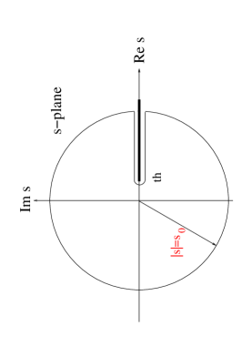
Figure 1: The contour underlying the chiral sum rules of Eq. (8)

$\Delta\overline{\Pi}_{V-A}(0)$ can be obtained either from the dispersive representation, or through the use of inverse-moment finite energy sum rules (IMFESRs). These are sum rules based on the integration, over the contour shown in Fig. 1, of the product $w(s)\,\tilde{\Pi}(s)$, where $w(s)$ is any function analytic in the region of the contour and $\tilde{\Pi}(s)\equiv\Pi(Q^{2})$ (with $Q^{2}\,=\,-s$) any correlator free of kinematic singularities. With $\rho(s)$ the spectral function of $\Pi(Q^{2})$, the resulting IMFESR relation is

$$w(0)\,\Pi(0)\,=\,{\frac{1}{2\pi i}}\,\oint_{|s|=s_{0}}ds\,{\frac{w(s)}{s}}\,\Pi(Q^{2})\ +\ \int_{th}^{s_{0}}ds\,{\frac{w(s)}{s}}\,\rho(s)\ \ ,$$ (8)

where $th$ is the threshold shown in Fig. 1. For large enough $s_{0}$, the Operator Product Expansion (OPE) representation of $\Pi(s)$ can be used in evaluating the first term on the RHS. The IMFESR relation is based on the same analyticity properties as the basic dispersion relation, the information on the integral from $s_{0}$ to $\infty$ in the dispersive representation being replaced, in the IMFESR approach, by the OPE approximation to the integral around the circle $|s|=s_{0}$. The added advantage of the IMFESR formulation lies in the freedom to choose the weight $w(s)$ in such a way as to improve various features of the evaluation of the RHS of Eq. (8).

Early continuum NLO determinations of $L_{10}^{r}$, using the IMFESR approach, were performed in Refs. dghs98 ; dominguez . Two NLO lattice determinations, based on analyses of low-Euclidean-$Q^{2}$ lattice data for $\Delta\Pi_{V-A}(Q^{2})$, also exist jlqcdvmanlo ; rbcukqcdvmanlo . The only $Q^{2}$-dependence of $\Delta\overline{\Pi}_{V-A}(Q^{2})$ at NLO lies in the loop contribution, ${\cal R}_{NLO}(Q^{2})$. It is now known that this dependence provides a very poor representation of the actual low-$Q^{2}$ behavior of $\Delta\overline{\Pi}_{V-A}(Q^{2})$ bgjmp13 (a similar observation was also made regarding the NLO representation of the $ud$ V correlator, $\Pi_{ud;V}(Q^{2})$, relevant to lattice determinations of the LO hadronic vacuum polarization contribution to the muon anomalous magnetic moment ab06 ). This raises obvious questions for the earlier NLO $L_{10}^{r}$ determinations.

The NNLO representation of $\Delta\overline{\Pi}_{V-A}(Q^{2})$, needed to extend the NLO continuum dispersive/IMFESR determinations to NNLO, has the form abt00

$$\left[\Delta\overline{\Pi}_{V-A}(Q^{2})\right]_{NNLO}\,=\,{\cal R}_{NNLO}(Q^{2})\,+\,c_{9}(Q^{2})L^{r}_{9}\,+\,c_{10}L^{r}_{10}\,+\,{\cal C}^{r}_{0}\,+\,{\cal C}^{r}_{1}\,-\,16C_{87}^{r}Q^{2}\ ,$$ (9)

where ${\cal R}_{NNLO}(Q^{2})$ is the sum of 1- and 2-loop contributions involving only LO vertices,

$$c_{10}\,=\,-8\left(1-8\mu_{\pi}-4\mu_{K}\right)\ ,$$ (10)

with $\mu_{P}={\frac{m_{P}^{2}}{32\pi^{2}f_{\pi}^{2}}}\,\log\left({\frac{m_{P}^{2}}{\hat{\mu}^{2}}}\right)$ the usual chiral logarithm and $f_{\pi}\simeq 92.2\ MeV$, $c_{9}(Q^{2})$ involves both chiral log and standard 1-loop, 2-propagator contributions, and

$${\cal C}^{r}_{0}\, =\,32m_{\pi}^{2}\left[C_{12}^{r}-C_{61}^{r}+C_{80}^{r}\right]$$

$${\cal C}^{r}_{1}\, =\,32\left(m_{\pi}^{2}+2m_{K}^{2}\right)\,\left[C_{13}^{r}-C_{62}^{r}+C_{81}^{r}\right]\ .$$ (11)

The $C_{k}^{r}$ here are the renormalized, dimensionful NNLO LECs defined in Ref. bce99 . The expression for ${\cal R}_{NNLO}(Q^{2})$, which is rather lengthy and hence not presented here, is readily reconstructed from the results quoted in Sections 4, 6 and Appendix B of Ref. abt00 , as is that for $c_{9}(Q^{2})$. $c_{10}$ and, for given $Q^{2}$, ${\cal R}_{NNLO}(Q^{2})$ and $c_{9}(Q^{2})$ are all fixed by the chiral scale $\mu$ and pseudoscalar decay constants and masses. The NNLO LECs in ${\cal C}^{r}_{0}$ are LO in $1/N_{c}$, while those in ${\cal C}^{r}_{1}$ are $1/N_{c}$-suppressed.

The NLO LEC $L_{9}^{r}$ has been accurately determined in an NNLO analysis of $\pi$ and $K$ electromagnetic form factors bt02 , and will be considered known in what follows. To simplify notation, we combine the known terms on the RHS of (9), defining

$$\hat{\cal R}_{NNLO}(Q^{2})\equiv{\cal R}_{NNLO}(Q^{2})\,+\,c_{9}(Q^{2})L_{9}^{r}\ .$$ (12)

Even with $L_{9}^{r}$ known, the NNLO representation of $\Delta\overline{\Pi}_{V-A}(0)$ depends on the two NNLO LEC combinations, ${\cal C}_{0}^{r}$ and ${\cal C}_{1}^{r}$, in addition to $L_{10}^{r}$. $L_{10}^{r}$ is thus no longer fixed by a determination of $\Delta\overline{\Pi}(0)_{V-A}$. Considering the $Q^{2}$-dependence of $\Delta\overline{\Pi}_{V-A}(Q^{2})$ does not help resolve this problem since the terms involving $L_{10}^{r}$, ${\cal C}^{r}_{0}$ and ${\cal C}^{r}_{1}$ in Eq. (9) are all $Q^{2}$-independent. Additional input on ${\cal C}_{0}^{r}$ and ${\cal C}_{1}^{r}$ is thus required to achieve a determination of $L_{10}^{r}$.

The ${\cal C}_{0}^{r}$ contribution to $\Delta\overline{\Pi}_{V-A}(0)$ is proportional to $m_{\pi}^{2}$ and expected to be small. In Ref. gapp08 , existing determinations of $C_{12}^{r}$ jopc12 and $C_{61}^{r}$ dk00 , and resonance ChPT (RChPT) estimates for $C_{80}^{r}$ abt00 ; up08 , were used to confirm this expectation. Neglect of the ${\cal C}_{1}^{r}$ contribution is far less safe since the ratio, $(m_{\pi}^{2}+2m_{K}^{2})/m_{\pi}^{2}\simeq 26$, of the prefactors in ${\cal C}_{1}^{r}$ and ${\cal C}_{0}^{r}$ more than compensates for the $1/N_{c}$ suppression of the NNLO LECs $C_{13,62,81}^{r}$ appearing in ${\cal C}_{1}^{r}$. Even more problematic is the fact that previous determinations exist for none of $C_{13,62,81}^{r}$, and that standard RChPT approaches yield no estimates for any of these LECs. This problem was dealt with in Ref. gapp08 by assigning to the $1/N_{c}$-suppressed combination $C_{13}^{r}(\mu_{0})-C_{62}^{r}(\mu_{0})+C_{81}^{r}(\mu_{0})$ (with $\mu_{0}$ the conventional chiral scale choice $\mu=0.77\ GeV$) a central value zero and error equal to $1/3=1/N_{c}$ of the value of the corresponding non-$1/N_{c}$-suppressed combination $C_{12}^{r}(\mu_{0})-C_{61}^{r}(\mu_{0})+C_{80}^{r}(\mu_{0})$ appearing in ${\cal C}_{0}^{r}$. Given the rather strong cancellations in the latter combination, this assumption is a far from conservative one. The uncertainty on the result for $L_{10}^{r}$ obtained after implementing this assumption in the NNLO representation of $\Delta\overline{\Pi}_{V-A}(0)$ turns out to be completely dominated by the assumed error on $C_{13}^{r}(\mu_{0})-C_{62}^{r}(\mu_{0})+C_{81}^{r}(\mu_{0})$. Improvements to this unsatisfactory situation can be achieved only through an independent determination of ${\cal C}_{1}^{r}$.

The fact that the coefficients of $L_{10}^{r}$, $C_{12}^{r}(\mu_{0})-C_{61}^{r}(\mu_{0})+C_{80}^{r}(\mu_{0})$ and $C_{13}^{r}(\mu_{0})-C_{62}^{r}(\mu_{0})+C_{81}^{r}(\mu_{0})$ in Eq. (9) depend differently on the pseudoscalar meson masses suggests disentangling the $L_{10}^{r}$, ${\cal C}_{0}^{r}$ and ${\cal C}_{1}^{r}$ contributions to $\Delta\overline{\Pi}_{V-A}(Q^{2})$ might be possible on the lattice, where variations in the pseudoscalar masses are easily accomplished through variations in the input quark masses. This paper shows how this possibility can be realized practically in an analysis using a combination of lattice and continuum results.

III Information from the Continuum Analysis of $\Delta\overline{\Pi}_{V-A}(Q^{2})$

The LECs $L_{10}^{r}$, ${\cal C}_{0}^{r}$ and ${\cal C}_{1}^{r}$ are very tightly constrained by (6). Inputting the results of Ref. abt00 for ${\cal R}_{NNLO}(0)$, and $L_{9}^{r}(\mu_{0})=0.00593(43)$ from Ref. bt02 , this constraint takes the form bgjmp13

$$L_{10}^{r}(\mu_{0})\,-\,0.0822\left[{\cal C}^{r}_{0}(\mu_{0})+{\cal C}^{r}_{1}(\mu_{0})\right]\,=\,-0.004098(59)_{exp}(74)_{L_{9}^{r}}$$ (13)

where the subscripts $exp$ and $L_{9}^{r}$ label contributions to the error on the RHS associated with that in (6), and the uncertainty on $L_{9}^{r}(\mu_{0})$, respectively.

Other information from the continuum analysis of Ref. bgjmp13 relevant to the analysis below concerns the range of validity of the NNLO representation. Crucial to the use of the lattice data is the ability to perform a chiral fit to the lattice data at non-zero Euclidean $Q^{2}$ and then use the results of that fit to reliably extrapolate to $Q^{2}=0$. This needs to be done for a range of pseudoscalar meson masses in order to allow the contributions of $L_{10}^{r}$, ${\cal C}_{0}^{r}$ and ${\cal C}_{1}^{r}$ to $\Delta\overline{\Pi}_{V-A}(0)$ to be disentangled. One thus needs to restrict one’s attention to lattice data at $Q^{2}$ for which the chiral representation being employed is reliable, and, of particular importance for our purposes, for which one knows the fit will produce a reliable determination of the $Q^{2}$-independent part of the representation, or, equivalently, $\Delta\overline{\Pi}_{V-A}(0)$.

As we will see in the next section, lattice errors on $\Delta\overline{\Pi}_{V-A}(Q^{2})$ turn out to be too large to allow the range of validity to be assessed using lattice data alone. Moreover, because, for Euclidean $Q^{2}$, $Q^{2}=0$ requires all components of $Q$ to be zero, the signal for the current-current two-point function vanishes on the lattice as $Q^{2}\rightarrow 0$. This means that $\Delta\overline{\Pi}_{V-A}(0)$ cannot be measured directly on the lattice, and that errors on $\Delta\overline{\Pi}_{V-A}(Q^{2})$ are necessarily large for very low $Q^{2}$.

The continuum dispersive approach, which produces significantly smaller errors on $\Delta\overline{\Pi}_{V-A}(Q^{2})$ in the low-$Q^{2}$ region relevant to the chiral analysis, and has no problem in determining $\Delta\overline{\Pi}_{V-A}(0)$ directly, is complementary in this regard. From Eq. (9), it is evident that, since ${\cal R}_{NNLO}(Q^{2})$ and $c_{9}(Q^{2})L_{9}^{r}$ are known, the NNLO form is characterized by two parameters, $C_{87}^{r}$ and the combination $c_{10}L_{10}^{r}+{\cal C}_{0}^{r}+{\cal C}_{1}^{r}$. In Ref. bgjmp13 it was found that the NNLO form produces a very accurate fit to the continuum data in a fit window covering the range from $Q^{2}=0$ to $\sim 0.1\ GeV^{2}$, one which, moreover, nicely reproduces the known value of $\Delta\overline{\Pi}_{V-A}(0)$. Extending the upper edge of the fit window beyond $\sim 0.1\ GeV^{2}$, one starts to see signs of curvature with respect to $Q^{2}$ beyond that present in the NNLO representation. This is especially evident in a drift in the fitted value for $C_{87}^{r}(\mu_{0})$ as the fit window is opened up, but also shows up in an accompanying small downward drift in the fitted result for $\Delta\overline{\Pi}_{V-A}(0)$ bgjmp13 . Curvature of $\Delta\overline{\Pi}_{V-A}(Q^{2})$ with respect to $Q^{2}$, beyond that produced by the nearly linear ${\cal R}_{NNLO}(Q^{2})$ contribution, would first appear at NNNLO in the chiral expansion, where it would be represented by a term of the form $CQ^{4}$, with the coefficient $C$ independent of the pseudoscalar meson masses at this order. Adding such a term to the NNLO form, stabilizes the fit results for $C_{87}^{r}$ as a function of the upper edge of the fit window, and restores the success of the resulting representation in reproducing the known value of $\Delta\overline{\Pi}_{V-A}(0)$ for fit windows with upper edges extending up to $\sim 0.3\ GeV^{2}$ bgjmp13 . This information motivates the restriction on the lattice data to be used in our analysis, described in the next section, to $Q^{2}<0.3\ GeV^{2}$.

IV The Lattice Data for $\Delta\overline{\Pi}_{V-A}(Q^{2})$

IV.1 Simulation Details

We consider data on $\Delta\overline{\Pi}_{V-A}(Q^{2})$ obtained from five RBC/UKQCD $n_{f}=2+1$ domain wall fermion (DWF) ensembles, three with Iwasaki gauge action, inverse lattice spacing $1/a\,=\,2.31\ GeV$, pion masses $m_{\pi}\,=\,293$, $349$ and $399\ MeV$, and $m_{\pi}L=4.1$, $4.8$, $5.5$, respectively, and two with Iwasaki+DSDR gauge action, $1/a\,=\,1.37\ GeV$, $m_{\pi}\,=\,171$ and $248\ MeV$ and $m_{\pi}L=4.0,\ 5.5$, respectively.

$Ensemble$	$V$	$\beta$	$a^{-1}\,{[GeV]}$	$Q^{2}_{min}\,{[GeV^{2}]}$	$am_{s}$	$am_{u}$	$m_{\pi}\,{[GeV]}$	$m_{K}\,{[GeV]}$	$F_{\pi}\,{[GeV]}$
E1	$32^{3}\times 64$	1.75	1.37(1)	0.018	0.045	0.001	0.171(1)	0.492(1)	0.130(2)
E2	$32^{3}\times 64$	1.75	1.37(1)	0.018	0.045	0.0042	0.248(1)	0.509(1)	0.139(2)
E3	$32^{3}\times 64$	2.25	2.31(4)	0.05	0.03	0.004	0.293(1)	0.561(1)	0.142(1)
E4	$32^{3}\times 64$	2.25	2.31(4)	0.05	0.03	0.006	0.349(1)	0.578(1)	0.148(1)
E5	$32^{3}\times 64$	2.25	2.31(4)	0.05	0.03	0.008	0.399(1)	0.596(1)	0.154(1)

Table 1: Parameters of the lattice ensembles used in our study. $m_{\pi}$, $m_{K}$ and $F_{\pi}$ are from ainv231 ($E3$-$E5$) and ainv137 ($E1,\,E2$).

The simulation parameters for the lattice calculations are summarized in Table 1. Along with the bare lattice simulation parameters, we also list the associated values of $m_{\pi}$, $m_{K}$ and $F_{\pi}\equiv\sqrt{2}f_{\pi}$, as well as the minimum $Q^{2}$ value attainable for each lattice, which is governed by its physical volume. Further details of the simulations for the three fine and two coarse ensembles may be found in Refs. ainv231 and  ainv137 , respectively.

The fine ensembles provide only three $Q^{2}$ values in the region $Q^{2}<0.3\ GeV^{2}$ employed in the current analysis. At the lowest of these, $Q^{2}\sim 0.05\ GeV^{2}$, the errors on $\Delta\overline{\Pi}_{V-A}(Q^{2})$, moreover, are so large that the result at this $Q^{2}$ plays no functional role in the analysis. The constraints obtained using these ensembles thus come from the two intermediate-$Q^{2}$ points. The coarse ensembles have improved low-$Q^{2}$ coverage, providing seven $Q^{2}$ values below $0.3\ GeV^{2}$, four with errors small enough that the corresponding data plays a role in the analysis.

IV.2 The Current-Current Two-Point Functions on the Lattice

In this work we will need to consider the standard lattice current-current two-point correlation functions, defined, in momentum space, for the $V$ and $A$ currents, by

$$\Pi^{\mu\nu}_{ud;V}(Q^{2}) \equiv Z_{V}\sum_{x}e^{\mathrm{i}Q\cdot x}\langle 0|\mathcal{V}^{\mu}(x)V^{\nu}(0)|0\rangle,$$ (14)

$$\Pi^{\mu\nu}_{ud;A}(Q^{2}) \equiv Z_{A}\sum_{x}e^{\mathrm{i}Q\cdot x}\langle 0|\mathcal{A}^{\mu}(x)A^{\nu}(0)|0\rangle,$$ (15)

where we use the standard flavor $ud$ DWF conserved vector ($\mathcal{V}^{\mu}$) and axial-vector ($\mathcal{A}^{\mu}$) currents Furman:1994ky at the sink. At the source we use the corresponding local currents, $V^{\mu}$ and $A^{\mu}$, and have hence included the vector and axial-vector renormalization constants, $Z_{V}$ and $Z_{A}$, in Eqs. (14) and (15). The values of $Z_{V}$ and $Z_{A}$ for each of our ensembles were determined in ainv231 ; ainv137 .

The two-point functions in Eqs. (14) and (15) can be decomposed into longitudinal ($J=0$) and transverse ($J=1$) components,

$$\Pi^{\mu\nu}_{ud;V/A}=\left(Q^{2}\delta_{\mu\nu}-Q_{\mu}Q_{\nu}\right)\Pi^{(1)}_{ud;V/A}(Q^{2})-Q_{\mu}Q_{\nu}\Pi^{(0)}_{ud;V/A}(Q^{2})\,.$$ (16)

On the lattice momenta are discretised, $Q_{\mu}=\frac{2\pi n_{\mu}}{L_{\mu}}$ where $n_{\mu}$ is a 4-tuple of integers, and $L_{\mu}$ is the length of the lattice in the $\mu$ direction. In what follows, we will use the lattice momentum

$$\hat{Q}_{\mu}=\frac{2}{a}\sin\left(\frac{\pi n_{\mu}}{L_{\mu}}\right).$$ (17)

and associate the quantity $\hat{Q}^{2}=\sum_{\mu}\hat{Q}_{\mu}^{2}$ with the continuum spacelike squared-momentum $Q^{2}$.

The two-point correlators used here are the same as those used previously in studies of the QCD S-parameter rbcukqcdvmanlo and the hadronic contribution to the anomalous magnetic moment of the muon Boyle:2011hu , and we refer the interested reader to those papers for more technical details.

IV.3 The Lattice V-A Results

In Table 1 we provide the values of $m_{\pi}$, $m_{K}$ and $F_{\pi}$ for each of the lattice ensembles. These are needed both for the $\pi$-pole subtraction, required to convert $\Delta\Pi_{V-A}(Q^{2})$ to $\Delta\overline{\Pi}_{V-A}(Q^{2})$, and in evaluating the 1- and 2-loop contributions to the NNLO representation of $\Delta\overline{\Pi}_{V-A}(Q^{2})$ for each of the ensembles. The error on the $\pi$-pole subtraction, produced by uncertainties in the ensemble values of $F_{\pi}$ and $m_{\pi}$, and that on $\Delta\Pi_{V-A}(Q^{2})$, are treated as independent in computing the error on $\Delta\overline{\Pi}_{V-A}(Q^{2})$. Results for further observables for the three fine ensembles may be found in Ref. ainv231 and for the two coarse ensembles in Ref. ainv137 . In what follows, we identify individual ensembles using the labels ($E1$–$E5$) introduced to specify them in the Table.

A comparison of the continuum (dispersive) results for $\Delta\overline{\Pi}_{V-A}(Q^{2})$ to those for ensemble $E1$ (whose $m_{\pi}$ value, $171\ MeV$, lies closest to the physical one) are shown in Fig. 2. We would expect these to be in good agreement, since the $\pi$ pole contribution, which depends more sensitively on $m_{\pi}$, has been subtracted in forming $\Delta\overline{\Pi}_{V-A}(Q^{2})$. The left panel shows the comparison in the low-$Q^{2}$ chiral fit region, $0<Q^{2}<0.3\ GeV^{2}$, the right panel the comparison for $Q^{2}\sim$ a few $GeV^{2}$. The agreement in both regions is good, suggesting lattice artifacts are well under control.

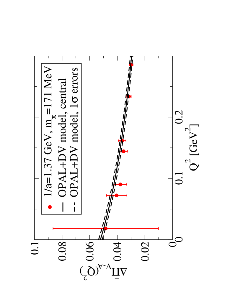
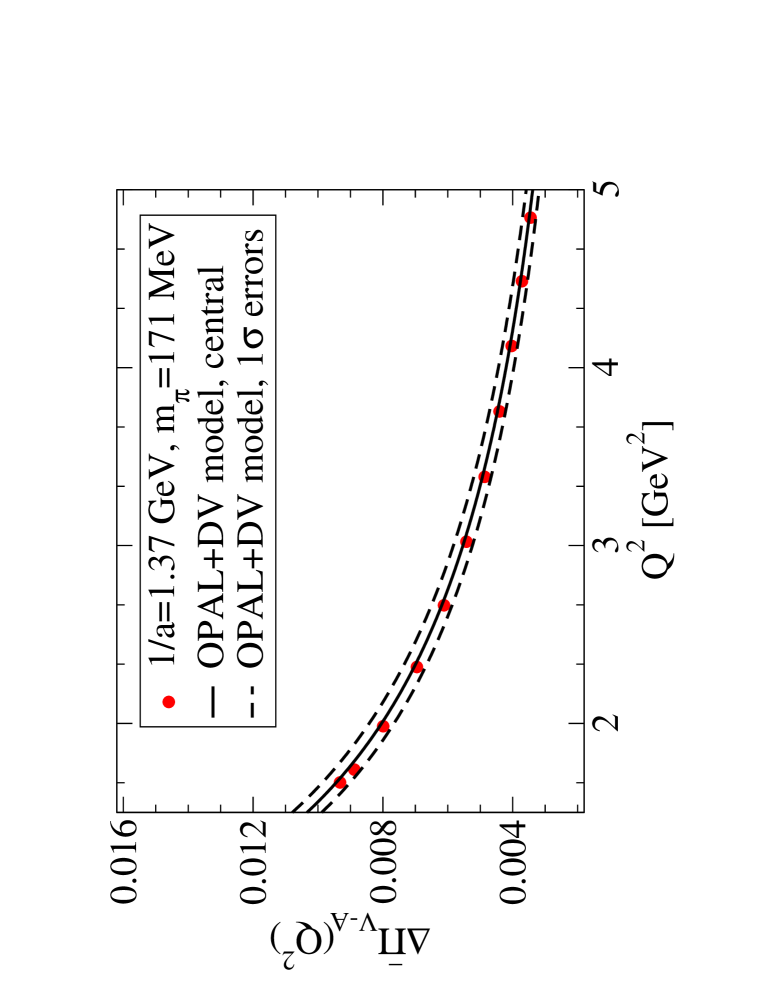
Figure 2: Comparison of continuum and $1/a=1.37\ GeV$, $m_{\pi}=171\ MeV$ ensemble lattice results for $\Delta\overline{\Pi}_{V-A}(Q^{2})$ in the low-$Q^{2}$ (left panel) and high-$Q^{2}$ (right panel) regions

Fig. 3 illustrates the problems that would be encountered if one attempted an NNLO analysis involving lattice data alone. The figure shows the values of $L_{10}^{r}(\mu_{0})$ obtained by assuming the validity of the NLO representation of $\Delta\overline{\Pi}_{V-A}(Q^{2})$ and using it to solve for $L_{10}^{r}$ at each $Q^{2}$. Results are shown for each of the four lightest $m_{\pi}$ ensembles ($E1-E4$). The measured values for the pseudoscalar masses and decay constants for the given ensemble ainv231 ; ainv137 (see Table 1) are taken as inputs in all cases. Also shown, for comparison, are the results obtained from a similar NLO analysis of the continuum results. The uncertainties on the continuum results (not shown explicitly) are small ($\sim 2.5\%$) and strongly correlated in the region of $Q^{2}$ shown in the figure.

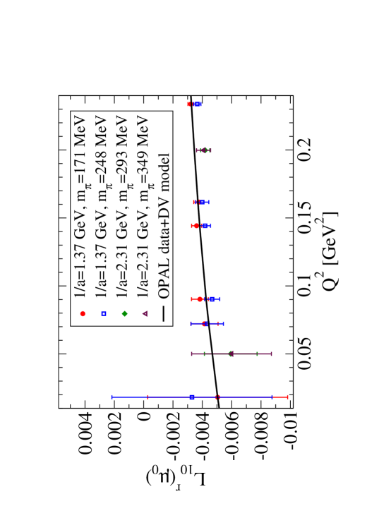
Figure 3: Point-by-point determinations of $L_{10}^{r}(\mu_{0})$, with $\mu_{0}=0.77\ GeV$, obtained assuming the validity of the NLO form, Eq. (7), for $\Delta\overline{\Pi}_{V-A}(Q^{2})$. Points with error bars are obtained from the lattice data discussed in the text, while the continuous curve results from applying the NLO form to the continuum dispersive results for $\Delta\overline{\Pi}_{V-A}(Q^{2})$.

While the incompatibility of the NLO form and the continuum results is immediately evident in the obvious non-constancy, within errors, of $L_{10}^{r}$ with respect to $Q^{2}$, it is far from clear that this would be the case if one had access only to the lattice results. In fact, if one imposes as input the (albeit non-conservative) assessment/assumptions of Ref. gapp08 regarding ${\cal C}_{0}^{r}$ and ${\cal C}_{1}^{r}$, a NNLO fit does become possible, and returns a value for the NNLO LEC $C_{87}^{r}$ (which accounts for the bulk of the $Q^{2}$-dependence of $\Delta\overline{\Pi}_{V-A}(Q^{2})$ in the low-$Q^{2}$ region) which is $\sim 2\sigma$ away from zero boylelatt13vma , showing that the lattice data is capable of distinguishing, to some extent, between the NLO and NNLO forms. The lattice errors are, however, much too large to allow a simultaneous fit of all four unknown LEC combinations $L_{10}^{r}$, $C_{87}^{r}$, ${\cal C}_{0}^{r}$ and ${\cal C}_{1}^{r}$.

To make progress, a way must be found to combine the lattice and continuum results, and take advantage of their complementary strengths. We discuss a practical way of accomplishing this goal in the next section.

V Combining Lattice and Continuum Data to Improve the Determination of $L_{10}^{r}$

It is convenient to reduce the number of unknown LECs to be dealt with by working with the difference of the physical-mass, continuum and corresponding lattice results for $\Delta\overline{\Pi}_{V-A}(Q^{2})$, evaluated at the same $Q^{2}$. With $L_{9}^{r}$ considered known bt02 , the resulting difference

$$\delta\Delta\overline{\Pi}(Q^{2})\equiv\left[\Delta\overline{\Pi}_{V-A}(Q^{2})\right]_{latt}\,-\,\left[\Delta\overline{\Pi}_{V-A}(Q^{2})\right]_{cont}\ ,$$ (18)

depends only on the LECs $L_{10}^{r}$, ${\cal C}_{0}^{r}$ and ${\cal C}_{0}^{r}$. Explicitly

$$\delta\Delta\overline{\Pi}(Q^{2})\,=\,\Delta\hat{\cal R}^{E}(Q^{2})\,+\,\Delta c_{10}^{E}\,L_{10}^{r}\,+\,\delta^{E}_{0}{\cal C}_{0}^{r}\,+\,\delta^{E}_{1}{\cal C}_{1}^{r}\ ,$$ (19)

where

$$\Delta\hat{\cal R}^{E}(Q^{2})\equiv\left[\hat{\cal R}_{NNLO}(Q^{2})\right]_{latt}^{E}\,-\,\left[\hat{\cal R}_{NNLO}(Q^{2})\right]_{phys}$$

$$\Delta c_{10}\equiv\left[c_{10}\right]_{latt}^{E}-\left[c_{10}\right]_{phys}$$

$$\delta_{0}\equiv\left[m_{\pi}^{2}\right]_{latt}^{E}/\left[m_{\pi}^{2}\right]_{phys}$$

$$\delta_{1}\equiv\left[m_{\pi}^{2}+2m_{K}^{2}\right]_{latt}^{E}/\left[m_{\pi}^{2}+2m_{K}^{2}\right]_{phys}\ ,$$ (20)

with the superscript $E$ labelling the ensemble under consideration and the subscripts $phys$ and $latt$ indicating the values of the quantities in question obtained using physical and lattice values for the relevant pseudoscalar masses and decay constants, respectively. $\delta\hat{\cal R}^{E}(Q^{2})$ and $\Delta c_{10}^{E}$ of course also depend on the chiral scale $\mu$.

With this notation, the combined lattice-continuum constraints, for a given ensemble $E$, become

$$\Delta c_{10}^{E}L_{10}^{r}\,+\,\delta_{0}^{E}{\cal C}_{0}^{r}\,+\,\delta_{1}^{E}{\cal C}_{1}^{r}\,=\,\delta\Delta\overline{\Pi}(Q^{2})\,-\,\Delta\hat{\cal R}^{E}(Q^{2})\,\equiv\,\Delta T^{E}(Q^{2})\ .$$ (21)

Since both terms on the RHS are $Q^{2}$-dependent, while the LHS is $Q^{2}$-independent, the versions of these constraints corresponding to different $Q^{2}$, but the same lattice ensemble $E$ can be used to provide checks on the self-consistency of the data employed, as well as on the reliability of the analysis framework. It turns out that the two constraints with reasonable errors obtained for the ensemble $E5$ do not pass this self-consistency test, while all of the available constraints are consistent for the other four ensembles. We thus exclude the ensemble $E5$ from the rest of the analysis. $E5$ is the ensemble with the largest pion mass, $m_{\pi}=399\ MeV$, a value which may, in any case, have been pushing the bounds of the chiral analysis. The consistency of the constraints for the other four ensembles is displayed in Fig. 4, which plots the $\Delta T^{E}(Q^{2})$ for these ensembles for the $Q^{2}$ of interest to the chiral analysis. The left panel shows the results for the fine $1/a=2.31\ GeV$ ensembles $E3$ and $E4$, the right panel the results for the coarse $1/a=1.37\ GeV$ensembles $E1$ and $E2$. The lowest $Q^{2}$ points, at $Q^{2}=0.018\ GeV^{2}$, have been omitted from the right panel since incorporating their absolutely enormous errors would force a dramatic increase in the range displayed on the vertical axis. In both panels, the $Q^{2}$ values for the ensemble with heavier value of $m_{\pi}$ have been shifted slightly to the right for presentational clarity.

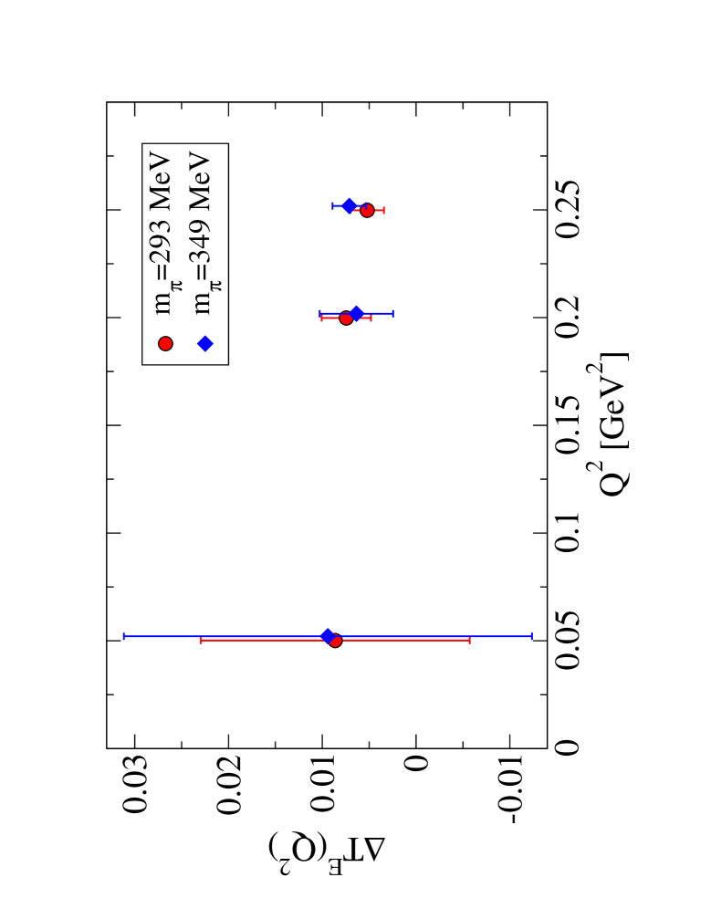
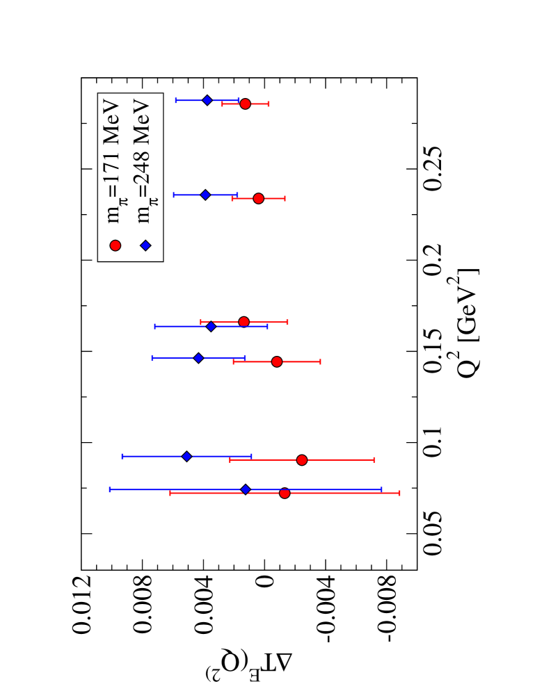
Figure 4: $\Delta T^{E}(Q^{2})$ as a function of $Q^{2}$ for the $1/a=2.31\ GeV$ ensembles $E3$ ($m_{\pi}=293\ MeV$) and $E4$ ($m_{\pi}=349\ MeV$) (left panel) and the $1/a=1.37\ GeV$ ensembles $E1$ ($m_{\pi}=171\ MeV$) and $E2$ ($m_{\pi}=248\ MeV$) (right panel)

For the remaining four ensembles employed in the analysis, a final combined version, $\Delta\overline{T}^{E}$, of the RHS of the constraint for each ensemble is obtained by performing a weighted average, over the points with $Q^{2}<0.3\ GeV^{2}$ available for that ensemble, of the corresponding $Q^{2}$-dependent RHSs. The average is more heavily weighted to the upper portion of the $Q^{2}$ analysis window, where the main source of error, that on $\Delta\overline{\Pi}_{V-A}(Q^{2})$, is smaller, and, given the good self-consistency, we assign to $\overline{T}^{E}$ an uncertainty typical of the errors in this region. The results of this exercise are

$$\Delta\overline{T}^{1}\,=\,0.0007(17)$$

$$\Delta\overline{T}^{2}\,=\,0.0039(21)$$

$$\Delta\overline{T}^{3}\,=\,0.0062(18)$$

$$\Delta\overline{T}^{4}\,=\,0.0070(18)\ .$$ (22)

Performing a combined fit incorporating the continuum $\Delta\overline{\Pi}_{V-A}(0)$ constraint, Eq. (13), and the four lattice-continuum constraints obtained by employing the results of Eqs. (22) on the RHS of Eq. (21), we find

$$L_{10}^{r}(\mu_{0})\,=\,-0.0031(8)$$

$${\cal C}_{0}^{r}(\mu_{0})\,=\,-0.0008(8)$$

$${\cal C}_{1}^{r}(\mu_{0})\,=\,\ \ 0.014(11)\ .$$ (23)

The size of the errors reflects the non-trivial size of the uncertainties on the $\Delta\overline{T}^{E}$ in (22), and the fact that the associated constraints, (21), are being required to provide information on two additional fit parameters. While the resulting errors, especially those on ${\cal C}_{0}^{r}$ and ${\cal C}_{1}^{r}$, are larger than one might hope, they have, at least, the advantage of being data-based.

The errors on the $\Delta\overline{T}^{E}$ in (22) result largely from those on the lattice data for $\Delta\overline{\Pi}_{V-A}(Q^{2})$. It is, unfortunately, difficult to significantly improve these, and thus necessary to look to additional continuum input for any further improvement. The existence of strong correlations amongst the fit parameters in (23) suggests that a single additional constraint should be sufficient to achieve a reduction in the errors for all three fit parameters. Fortunately, such an additional constraint exists.

The source of this constraint is a recent IMFESR analysis kmimfesr13 of the flavor-breaking (FB) correlator difference

$$\delta^{FB}\Delta\overline{\Pi}_{V-A}(Q^{2})\,\equiv\,\overline{\Pi}^{(0+1)}_{ud;V-A}(Q^{2})-\overline{\Pi}^{(0+1)}_{us;V-A}(Q^{2})\ ,$$ (24)

from which the result

$$\delta^{FB}\Delta\overline{\Pi}_{V-A}(0)\,=\,0.0113(15)$$ (25)

was obtained. The analysis employed (i) OPAL non-strange spectral data for the $V$ and $A$ channels opalud99 , updated as in Ref. dv72 ; (ii) $us$ spectral data from ALEPH alephus99 and the recent B-factory results for the exclusive mode $K^{-}\pi^{0}$ babarkmpi0 , $K_{s}\pi^{-}$ bellekspi , $K^{-}\pi^{+}\pi^{-}$ babarkpipiallchg and $K_{s}\pi^{-}\pi^{0}$ bellekspipi invariant mass distributions measured in strange hadronic $\tau$ decays; and (iii) PDG pdg12 , FLAG flag , and additional lattice davies12 ; boyled2convlatt results for the treatment of, and input to, OPE contributions. The $us$ exclusive mode distributions are normalized to current strange $\tau$ branching fractions. We refer the reader to Ref. kmimfesr13 for details of the analysis.

The result given in Eq. (25) is of interest for our purposes because the NNLO LEC contributions to the NNLO representation of $\delta^{FB}\Delta\overline{\Pi}_{V-A}(0)$ appear in precisely the combination ${\cal C}_{0}^{r}$. Explicitly,

$$\left[\delta^{FB}\Delta\overline{\Pi}_{V-A}(0)\right]_{NNLO}\,=\,{\cal R}^{FB}(0)+d^{FB}_{5}L_{5}^{r}+d^{FB}_{9}L_{9}^{r}+d^{FB}_{10}L_{10}^{r}+\left({\frac{m_{K}^{2}-m_{\pi}^{2}}{m_{\pi}^{2}}}\right)\,{\cal C}_{0}^{r}\ ,$$ (26)

where ${\cal R}^{FB}(Q^{2})$ represents the sum of all 1- and 2-loop contributions with only LO vertices. The (rather lengthy) expression for ${\cal R}^{FB}(0)$, as well as those for the $Q^{2}$-independent coefficients $d^{FB}_{5,9,10}$, are obtainable from the results quoted in Ref. abt00 and not presented here. They are fully fixed once the chiral scale $\mu$ and pseudoscalar masses and decay constants are specified.

Unlike the case of the NNLO representation of $\Delta\overline{\Pi}_{V-A}(0)$, where the coefficient $c_{10}$ of $L_{10}^{r}$ in Eq. (9) contains both NLO and NNLO contributions, NLO contributions proportional to $L_{10}^{r}$ cancel in forming the FB difference $\delta^{FB}\Delta\overline{\Pi}_{V-A}(Q^{2})$. The result is that $d^{FB}_{10}$ is purely NNLO, and suppressed numerically compared to $c_{10}$. The coefficient of ${\cal C}_{0}^{r}$ in Eq. (26) is, in contrast, enhanced by the factor $(m_{K}^{2}-m_{\pi}^{2})/m_{\pi}^{2}\simeq 11.6$. The linear combination of $L_{10}^{r}$ and ${\cal C}_{0}^{r}$ appearing in (26) is thus very different from that appearing in the continuum $\Delta\overline{\Pi}_{V-A}(0)$ constraint. Since $L_{9}^{r}$ is well known bt02 , and $L_{5}^{r}$, which is also known bj11 , is such that its contribution to the RHS of (26) is numerically small, the result obtained by combining Eqs.(25), and (26),

$$2.12\,L_{10}^{r}(\mu_{0})\,+\,11.6\,{\cal C}_{0}^{r}(\mu_{0})\,=\,-0.00346\,(161)\ ,$$ (27)

provides the additional independent constraint we need.

We now have the two continuum constraints, Eqs. (13) and (27), and four combined lattice-continuum constraints, Eq. (21). All of these can be cast in the form

$$a_{10}^{(k)}L_{10}^{r}\,+\,a_{0}^{(k)}{\cal C}_{0}^{r}\,+\,a_{1}^{(k)}{\cal C}_{1}^{r}\,=\,d^{(k)}\pm\delta d^{(k)}\,,$$ (28)

with $k$ labelling the different constraints, the $a_{10}^{(k)}$, $a_{0}^{(k)}$ and $a_{1}^{(k)}$ all known, and $\delta d^{(k)}$ the relevant error. For the four lattice-continuum constraints, $\delta d^{(k)}$ is totally dominated by the error on the lattice determination of the $\Delta\overline{\Pi}_{V-A}(Q^{2})$ for the ensemble in question. For the continuum $V-A$ constraint, Eq. (13), $\delta d^{(k)}$ is determined by the experimental errors on the $ud$ $V-A$ spectral distribution. Finally, for the FB continuum constraint, Eq. (27), $\delta d^{(k)}$ is dominated by the experimental errors on the $us$ spectral distribution and $us$ $V/A$ separation uncertainties. Since the dominant sources of error for the different constraints are independent, we fit $L_{10}^{r}(\mu_{0})$, ${\cal C}_{0}(\mu_{0})$ and ${\cal C}_{1}(\mu_{0})$ by minimizing

$$\chi^{2}\,=\,\sum_{k}{\frac{\left[d_{k}\,-\,\left(a_{10}^{(k)}\,L_{10}^{r}(\mu_{0})\,+\,a_{0}^{(k)}\,{\cal C}_{0}(\mu_{0})\,+\,a_{1}^{(k)}\,{\cal C}_{1}(\mu_{0})\right)\right]^{2}}{\left[\delta d^{(k)}\right]^{2}}}\ .$$ (29)

Implementing this six-constraint fit, we find the significantly improved results

$$L_{10}^{r}(\mu_{0})\,=\,-0.00346\,(29)_{fit}(13)_{L_{5,9}^{r}}$$

$${\cal C}_{0}^{r}(\mu_{0})\,=\,-0.00034\,(13)_{fit}(3)_{L_{5,9}^{r}}$$

$${\cal C}_{1}^{r}(\mu_{0})\,=\,\ 0.0081(35)_{fit}(7)_{L_{5,9}^{r}}\ ,$$ (30)

where we have separated out the contributions to the errors from the uncertainties on the input values for $L_{5}^{r}(\mu_{0})$ and $L_{9}^{r}(\mu_{0})$. The resulting ${\cal C}^{r}_{0}(\mu_{0})$-${\cal C}^{r}_{1}(\mu_{0})$, ${\cal C}^{r}_{0}(\mu_{0})$-$L_{10}^{r}(\mu_{0})$ and ${\cal C}^{r}_{1}(\mu_{0})$-$L_{10}^{r}(\mu_{0})$ correlations are $-0.045$, $0.012$ and $0.978$, respectively. The results (30) update the preliminary versions presented in Ref. boyleetalvmalatt13 , and represent the best determination of $L_{10}^{r}$ to date.

VI Summary and Discussion

Our main results are those given in Eq. (30), where the error labelled by the subscript $fit$ is that resulting from the errors on the two continuum and four lattice-continuum constraints employed in the combined fit. The key result is that for $L_{10}^{r}(\mu_{0})$, though that for ${\cal C}_{1}^{r}(\mu_{0})$ provides a further example of a NNLO LEC combination vanishing in the large-$N_{c}$ limit which cannot be neglected for $N_{c}=3$.

It is worth commenting on the absence of constraints from the two RBC/UKQCD ensembles with $1/a=1.75\ GeV$ in our analysis. These ensembles provide five $Q^{2}<0.3\ GeV^{2}$, three with errors small enough to be useful in assessing the self-consistency of the $\Delta T^{E}(Q^{2})$. The three low-error $\Delta T^{E}(Q^{2})$ for the ensemble with $m_{\pi}=333\ MeV$, unfortunately, fail the self-consistency test. Those for the ensemble with $m_{\pi}=423\ MeV$ pass the self-cnsistency test, but correspond to an $m_{\pi}$ which is both potentially rather large for use in an NNLO analysis and significantly larger than the largest value, $m_{\pi}=349\ MeV$, employed in the analysis discussed above. We can, however, use the results for the heavy $m_{\pi}$ ensemble to further test that the $m_{\pi}<350\ MeV$ employed above lie safely within the range of validity of the NNLO analysis framework. To do so we have performed an extended version of the analysis above, adding in the additional combined lattice-continuum constraint $\Delta\bar{T}^{6}=0.0048(17)$ obtained for the $1/a=1.75\ GeV$, $m_{\pi}=423\ MeV$ ensemble. The expanded fit yields results, ${\cal C}_{0}^{r}(\mu_{0})\,=\,-0.0036(12)$, ${\cal C}_{1}^{r}(\mu_{0})\,=\,0.0070(24)$ and $L_{10}^{r}(\mu_{0})\,=\,-0.00355(23)$, in excellent agreement with those of the main analysis. Since $m_{\pi}=423\ MeV$ is rather large, we do not use the results of this extended analysis as our main ones, but do argue that the stability of the results with respect to such a large increase in the maximum $m_{\pi}$ employed provides strong evidence in support of the reliability of our NNLO treatment of the lower-$m_{\pi}$ data.

The only other NNLO determination of $L_{10}^{r}(\mu_{0})$ we are aware of is that of Ref. gapp08 . The central value in this case, $L_{10}^{r}(\mu_{0})\,=\,-0.00406(39)$, differs from ours by $\sim 2\sigma$. The difference results, essentially entirely, from the difference in ${\cal C}_{1}^{r}(\mu_{0})$ values, with ${\cal C}_{1}^{r}(\mu_{0})$ (then unknown) having been assigned the (assumed) central value $0$ in gapp08 , but fit, using lattice data, in our analysis. The error on $L_{10}^{r}(\mu_{0})$ in Ref. gapp08 , as stressed in that reference, is completely dominated by the assumed uncertainty on ${\cal C}_{1}^{r}(\mu_{0})$. This uncertainty is based on the assumption that

$$|C_{13}^{r}(\mu_{0})-C_{62}^{r}(\mu_{0})+C_{81}^{r}(\mu_{0})|\,<\,|C_{12}^{r}(\mu_{0})-C_{61}^{r}(\mu_{0})+C_{80}^{r}(\mu_{0})|/3\ ,$$ (31)

which turns out to be insufficiently conservative, and would be even more so were the data-based result obtained above for ${\cal C}_{0}^{r}(\mu_{0})$ (which is $\sim-0.6$ times that employed in Ref. gapp08 ) to be used on the RHS. Our error has the advantage not only of being smaller, but of being based entirely on lattice and continuum data errors and independent of any additional assumptions.

It is useful to clarify the relative roles of the lattice-continuum and continuum constraint errors, since this determines where best to focus future efforts to further reduce the error on $L_{10}^{r}$. In this context, it is also relevant to bear in mind that the $\delta^{FB}\Delta\overline{\Pi}_{V-A}(0)$ constraint, Eq. (27), which is crucial in achieving the reduced errors in (30), relies on current strange hadronic $\tau$ decay mode branching fractions for the normalizations of the exclusive strange mode contributions to the $us$ $V-A$ spectral function. These branching fractions, as well as the exclusive strange distributions, remain the subjects of ongoing experimental investigation. In addition, the $V/A$ separation of the exclusive $K\pi\pi$ mode spectral contributions, which is currently done only approximately, can, in principle, be improved through angular analyses km92 which are feasible with B-factory data. Improvements to the FB IMFESR analysis, and hence to the associated FB $V-A$ constraint, are thus likely to be accessible in the near future.

In order to illustrate the impact plausible changes in the $us$ $V-A$ spectral data might have on $L_{10}^{r}$, we have rerun the analysis described in Sec. V using as input to the FB $V-A$ IMFESR constraint, the alternate value, $\delta^{FB}\Delta\overline{\Pi}_{V-A}(0)\,=\,0.0098(15)$, obtained in Ref. kmimfesr13 using the alternate, still-preliminary BaBar results for the branching fractions $B[\tau^{-}\rightarrow K^{-}\,n\,\pi^{0}\nu_{\tau}]$, $n=1,2,3$, reported in Ref. adametz . The results of this exercise are $L_{10}^{r}(\mu_{0})\,=\,-0.00356(32)$, ${\cal C}_{0}^{r}(\mu_{0})\,=\,-0.00024(12)$ and ${\cal C}_{1}^{r}(\mu_{0})\,=\,0.0068(32)$. While the input constraint value has been shifted by $1\,\sigma$, $L_{10}(\mu_{0})$ has shifted by only $\sim 1/3$ of the $fit$ component of the error in the main result. We learn from this exercise that, at present, it is the lattice errors on $\Delta\overline{\Pi}_{V-A}(Q^{2})$ which dominate the uncertainty on $L_{10}^{r}$. Improvements in the error on the FB $V-A$ IMFESR constraint (the less precise of the two continuum constraints), though almost certainly feasible in the near future, will not help to significantly reduce the error on $L_{10}^{r}$. Further non-trivial improvement requires instead a reduction in the errors on the lattice determinations of $\Delta\overline{\Pi}_{V-A}(Q^{2})$. A natural target in this regard is a reduction in the errors on the $\pi$ pole subtraction through a reduction in the errors on $f_{\pi}$ for the two coarse $1/a=1.37\ GeV$ ensembles, where these errors on the $f_{\pi}^{2}$ factor entering this subtraction are currently a factor of $\sim 2.3$ larger than those for the fine $1/a=2.31\ GeV$ ensembles.

Our determination of $L_{10}^{r}$ allows us to also fix the corresponding $SU(2)\times SU(2)$ LEC, $\ell_{5}^{r}$, whose relation to $L_{10}^{r}$ at NNLO has been worked out in Ref. ghis07 . With $F_{0}$ the $\pi$ decay constant in the $SU(3)$ chiral limit, $\hat{m}_{K}$ the $K$ mass in the limit $m_{u,d}\rightarrow 0$, $\ell_{K}\equiv\log\left({\frac{\hat{m}_{K}^{2}}{\mu_{0}^{2}}}\right)$, $\nu_{K}\equiv{\frac{1}{32\pi^{2}}}\,\left(\ell_{K}+1\right)$ and $X\equiv{\frac{\hat{m}_{K}^{2}}{16\pi^{2}F_{0}^{2}}}$, this relation takes the form ghis07

$$\ell_{5}^{r}(\mu_{0})\,= \,\left(1-2X\ell_{K}\right)\,L_{10}(\mu_{0})+{\frac{1}{12}}\nu_{K}\,+\,X\,(0.000339+0.002243\ell_{K}-0.000396\ell_{K}^{2})$$ (32)

$$\qquad-\,X\,\ell_{K}\,L_{9}^{r}(\mu_{0})\,-\,8\hat{m}_{K}^{2}\,\left[C_{13}^{r}(\mu_{0})-C_{62}^{r}(\mu_{0})+C_{81}^{r}(\mu_{0})\right]\ ,$$

where, in writing the second line, we have converted the dimensionless versions of the NNLO LECs used in Ref. ghis07 to the dimensionful versions of Ref. bce99 used above. Note that the last term in this relation is proportional to the combination ${\cal C}_{1}^{r}$ determined above. Estimating $\hat{m}_{K}$ using the LO relation $\hat{m}_{K}^{2}=\bar{m}_{K}^{2}-{\frac{1}{2}}m_{\pi}^{2}$ (with $\bar{m}_{K}$ the average of the charged and neutral $K$ masses), and taking $F_{0}\simeq 80\ MeV$ from the $n_{f}=2+1$ lattice results favored by the FLAG assessment flag , we obtain

$$\ell_{5}^{r}(\mu_{0})\,=\,1.430\,L_{10}(\mu_{0})\,-\,0.00046\,+\,0.215\,L_{9}^{r}(\mu_{0})\,-\,{\frac{\hat{m}_{K}^{2}}{4(2m_{K}^{2}+m_{\pi}^{2})}}\,{\cal C}_{1}^{r}(\mu_{0})\ .$$ (33)

With the input of Ref. bt02 for $L_{9}^{r}(\mu_{0})$, we obtain, taking into account the $0.978$ correlation between the fitted values of $L_{10}^{r}(\mu_{0})$ and ${\cal C}_{1}^{r}(\mu_{0})$,

$$\ell_{5}^{r}(\mu_{0})\,=\,-0.00507(10)\ .$$ (34)

The uncertainty on $L_{9}^{r}(\mu_{0})$ plays no role to the number of significant figures quoted for the error. The result (34) corresponds to the value

$$\bar{\ell}_{5}\,=\,13.0\,(2)$$ (35)

for the scale-invariant coupling $\bar{\ell}_{5}$ defined in Ref. gl84 . This is not only in excellent agreement with the results $\bar{\ell}_{6}=16.0(5)(7)$ and $\bar{\ell}_{6}-\bar{\ell}_{5}=3.0(3)$ quoted in Ref. bijnenscd12 , arising from the NNLO $SU(2)\times SU(2)$ analyses of the $\pi$ vector form factor bct98 and $\pi^{+}\rightarrow e^{+}\nu_{e}\gamma$ bt97 , respectively, but, when combined with $\bar{\ell}_{6}-\bar{\ell}_{5}=3.0(3)$, in fact yields the somewhat improved determination $\bar{\ell}_{6}=16.0(4)$ for $\bar{\ell}_{6}$.

We close by comparing our results to RChPT estimates for the LECs/LEC combinations determined in our analysis, RChPT being the framework most often used to make such estimates in the literature. Large-$N_{c}$-based RChPT estimates L10rLONc for $L_{10}^{r}$ are scale-independent, and usually taken to correspond to $\mu\simeq\mu_{0}$. The resulting $L_{10}^{r}(\mu_{0})$ ($\simeq-0.0054$) is significantly more negative than indicated by our determination. The lack of scale-dependence in the large-$N_{c}$ version of the RChPT LEC predictions can be repaired by going beyond leading order in $1/N_{c}$. This has been done for the $V-A$ correlator in Ref. prsc08 , where $1/N_{c}$ corrections were shown to lower the RChPT prediction for $L_{10}^{r}(\mu_{0})$ prsc08 . The resulting prediction, with the scale-dependence now fully under control, is $-0.0044(9)$, compatible within errors with our result above. Large-$N_{c}$ RChPT predictions for the NNLO LECs entering the combination ${\cal C}_{0}^{r}$ abt00 ; up08 ; bj11 ; ceekpp05 ; km06 lead to a result ${\cal C}_{0}^{r}(\mu_{0})\simeq-0.0004$, in good agreement with the result above. This agreement, however, results from a fortuitous cancellation, with RChPT predictions for the individual $C_{12}^{r},\,C_{61}^{r}$ and $C_{80}^{r}$ differing significantly from the coupled channel dispersive result of Ref. jopc12 for $C_{12}^{r}(\mu_{0})$, and the results for $C_{61}^{r}(\mu_{0})$ and $C_{80}^{r}(\mu_{0})$ obtained in Ref. kmimfesr13 using FB IMFESRs in combination with the results of our fit above. The large-$N_{c}$ RChPT prediction for the $1/N_{c}$-suppressed LEC combination ${\cal C}_{1}^{r}$ is, of course, zero. To the best of our knowledge, $1/N_{c}$-corrections have not yet been investigated for any of the NNLO LECs.

- (1) S. Weinberg, Physica A96, 327 (1979).
- (2) J. Gasser and H. Leutwyler, Ann. Phys. 158, 142 (1984).
- (3) J. Gasser and H. Leutwyler, Nucl. Phys. B250, 465 (1985).
- (4) M.E. Peskin and T. Takeuchi, Phys. Rev. Lett. 65, 964 (1990).
- (5) M. Davier, L. Girlanda, A. Höcker and J. Stern, Phys. Rev. D58, 096014 (1998) [hep-ph/9802447].
- (6) C.A. Dominguez and K. Schilcher, Phys. Lett. B448, 93 (1999) [hep-ph/9811261] and ibid. B581, 193 (2004) [hep-ph/0309285]; J. Bordes, C.A. Dominguez, J. Penarrocha and K. Schilcher, JHEP 02, 037 (2006) [hep-ph/0511293].
- (7) M. González-Alonso, A. Pich and J. Prades, Phys. Rev. D78, 116012 (2008) [arXiv:0810.0760 (hep-ph)].
- (8) D. Boito et al., Phys. Rev. D87, 094008 (2013) [arXiv:1212.4471 (hep-ph)].
- (9) E. Shintani, et al., Phys. Rev. Lett. 101, 202004 (2008) [arXiv:0806.4222 (hep-lat)].
- (10) P.A. Boyle, L. Del Debbio, J. Wennekers and J.M. Zanotti [RBC and UKQCD Collaborations], Phys. Rev. D81, 014504 (2010) [arXiv:0909.4931 (hep-lat)].
- (11) P.A. Boyle et al., PoS LATTICE 2012, 156 (2012) [arXiv:1301.2565 (hep-lat)].
- (12) M. Golterman, K. Maltman and S. Peris, Phys. Rev. D89, 054036 (2014) [arXiv:1402.1043 (hep-ph)].
- (13) Y.-S. Tsai, Phys. Rev. D4, 2821 (1971).
- (14) J. Erler, Rev. Mex. Fis. 50, 200 (2004) [hep-ph/0211345].
- (15) J.H. Kühn and E. Mirkes, Z. Phys. C56, 661 (1992); Erratum: ibid. C67, 364 (1995).
- (16) K. Ackerstaff et al. [OPAL Collaboration], Eur. Phys. J. C7, 571 (1999) [hep-ex/9808019].
- (17) R. Barate, et al. [ALEPH Collaboration], Z. Phys. C76, 15 (1997); R. Barate, et al. [ALEPH Collaboration], Eur. Phys. J C4, 409 (1998); S. Schael et al. [ALEPH Collaboration], Phys. Rep. 421, 191 (2005) [hep-ex/0506072].
- (18) D. Boito, it et al., Phys. Rev. D85, 093015 (2012) [arXiv:1203.3146 (hep-ph)].
- (19) D. Boito, et al., Nucl. Phys. Proc. Suppl. 218, 104 (2011) [arXiv:1011.4426 (hep-ph)].
- (20) M. Davier, et al., arXiv:1312.1501 (hep-ex).
- (21) D. Boito, it et al., Phys. Rev. D84, 113006 (2011) [arXiv:1110.1127 (hep-ph)].
- (22) G. Amoros, J. Bijnens and P. Talavera, Nucl. Phys. B568, 319 (2000) [hep-ph/9907264].
- (23) C. Aubin and T. Blum, Phys. Rev. D75, 114502 (2006) [hep-lat/0608011].
- (24) J. Bijnens, G. Colangelo and G. Ecker, JHEP 02, 020 (1999) [hep-ph/9902437]; Ann. Phys. 280, 100 (2000) [hep-ph/9907333].
- (25) J. Bijnens and P. Talavera, JHEP 0203, 046 (2002) [hep-ph/0203049].
- (26) M. Jamin, J.A. Oller and A. Pich, JHEP 0402, 047 (2004) [hep-ph/0401080].
- (27) S. Dürr and J. Kambor, Phys. Rev. D61, 114025 (2000) [hep-ph/9907539].
- (28) R. Unterdorfer and H. Pichl, Eur. Phys. J. C55, 273 (2008) [arXiv:0801.2482 (hep-ph)].
- (29) Y. Aoki et al., Phys. Rev. D83, 074508 (2011) [arXiv:1011.0892 (hep-lat)].
- (30) R. Arthur et al., Phys. Rev. D87, 094514 (2013) [arXiv:1208.4412 (hep-lat)].
- (31) V. Furman and Y. Shamir, Nucl. Phys. B 439, 54 (1995) [hep-lat/9405004].
- (32) P. Boyle, L. Del Debbio, E. Kerrane and J. Zanotti, Phys. Rev. D 85, 074504 (2012) [arXiv:1107.1497 (hep-lat)].
- (33) R. Barate et al., Eur. Phys. J. C11 599 (1999) [hep-ex/9903015].
- (34) B. Aubert, et al. [The BaBar Collaboration], Phys. Rev. D76 051104 (2007) [arXiv:0707.2922 (hep-ex)].
- (35) D. Epifanov, et al. [The Belle Collaboration], Phys. Lett. B654 65 (2007) [arXiv:0706.2231 (hep-ex)].
- (36) I.M. Nugent, arXiv:1301.7105 (hep-ex).
- (37) S. Ryu, for the Belle Collaboration, arXiv:1302.4565 (hep-ex).
- (38) J. Beringer, et al., Phys. Rev. D86 010001 (2012).
- (39) For the main page of the 2013 FLAG compilation, see itpwiki.unibe.ch/ flag/index.php/ Review_of_lattice_result_concerning_low_energy_particle_physics.
- (40) C. McNeile, et al., Phys. Rev. D87 034503 (2013) [arXiv:1211.6577 (hep-lat)].
- (41) P.A. Boyle et al., PoS Confinement X, 100 (2012) [arXiv:1301.4930 (hep-ph)] and arXiv:1312.1716 (hep-ph).
- (42) J. Bijnens and I. Jemos, Nucl. Phys. B854 631 (2012) [arXiv:1103.5945 (hep-ph)].
- (43) P.A. Boyle et al., PoS (Lattice 2013), in press, [arXiv:1311.0397 (hep-ph)].
- (44) C. Allton et al. [RBC-UKQCD Collaboration], Phys. Rev. D78, 114509 (2008) [arXiv:0804.0473 (hep-lat)].
- (45) A. Adametz, “Measurement of decays into charged hadrons accompanied by neutral mesons and determination of the CKM matrix element ”, University of Heidelberg PhD thesis, July 2011, and the BaBar Collaboration, in progress.
- (46) J. Gasser, C. Haefeli, M.A. Ivanov and M. Schmid, Phys. Lett. B652 21 (2007) [arXiv:0706.0955 (hep-ph)].
- (47) J. Bijnens, PoS CD12 002 (2013) [arXiv:1301.6953 (hep-ph)].
- (48) J. Bijnens, G. Colangelo and P. Talavera, JHEP 05 014 (1998) [hep-ph/9805389].
- (49) J. Bijnens and P. Talavera, Nucl. Phys. B489 387 (1997) [hep-ph/9610269].
- (50) G. Ecker, J. Gasser, A. Pich and E. de Rafael, Nucl. Phys. B321 311 (1989); M.Knecht and A. Nyffeler, Eur. Phys. J. C21 659 (2001) [hep-ph/0106034]; V. Cirigliano et al., Nucl. Phys. B753 (2006) 139 [hep-ph/0603205]. See also Ref. abt00 .
- (51) A. Pich, I. Rosell and J.J. Sanz-CIllero, JHEP 07 014 (2008) [arXiv:0803.1567 (hep-ph)].
- (52) V. Cirigliano, et al., JHEP 04 006 (2005) [hep-ph/0503108)].
- (53) K. Kampf and B. Moussallam, Eur. Phys. J. C47 723 (2006) [hep-ph/0604125].