Convective Overstability in radially stratified accretion disks under thermal relaxation

Abstract

This letter expands the stability criterion for radially stratified, vertically unstratified accretion disks incorporating thermal relaxation. We find a linear amplification of epicyclic oscillations in these disks that depends on the effective cooling time, i.e. an overstability. The growth rates of the overstability vanish for both extreme cases, e.g. infinite cooling time and instantaneous cooling, i.e. the adiabatic and fully isothermal cases. However, for thermal relaxation times $\tau$ on the order of the orbital frequency, $\tau\Omega\sim 1$, modes grow at a rate proportional to the square of the Brunt-Väisälä  frequency. The overstability is based on epicyclic motions, with the thermal relaxation causing gas to heat while radially displaced inwards, and cool while radially displaced outwards. This causes the gas to have a lower density when moving outwards compared to when it moves inwards, so it feels the outwards directed pressure force more strongly on that leg of the journey. We suggest the term “Convective Overstability” for the phenomenon that has already been numerically studied in the non-linear regime in the context of amplifying vortices in disks, under the name “Subcritical Baroclinic Instability”. The point of the present paper is to make clear that vortex formation in three-dimensional disks is neither subcritical, i.e. does not need a finite perturbation, nor is it baroclinic in the sense of geophysical fluid dynamics, which requires on vertical shear. We find that Convective Overstability is a linear instability that will operate under a wide range of physical conditions for circumstellar disks.

1 Introduction

The hydrodynamical stability of circumstellar accretion disks has been a long-standing problem in astrophysics because turbulence appears to be needed to drive observed accretion flows (Shakura & Sunyaev, 1973). However, these disks are strongly stabilized by rotation and vertically stable stratification. While the identification of the role of Magneto-Rotational Instability in accretion disks (MRI, Velikhov 1959; Balbus & Hawley 1991) finally provided an incontrovertible linear instability, it was soon noted (Gammie, 1996) that significant portions of circumstellar disks are too poorly ionized to allow the MRI to act. The upper and outer edges for MRI turbulence appear to be set by ambipolar diffusion (Perez-Becker & Chiang, 2011; Bai, 2011) and by the stiffness of the fields at high magnetic pressure (Miller & Stone, 2000; Kim & Ostriker, 2000; Turner et al., 2010). These obstacles of the otherwise robust MRI continue to motivate studies of hydrodynamical instabilities.

The radial temperature structure of modestly accreting circumstellar disks are largely controlled by irradiation from the central star, although any accretion flow will lead to increased heating and dependent on the local opacity to a non trivial radial temperature and density profile (Bell et al., 1995; D’Alessio et al., 2005). The radial temperature gradient can overpower the expected density gradient, leading to a negative radial entropy gradient (Klahr et al., 2013), which can drive the formation of vortices through a baroclinic mechanism, e.g. the non-vanishing baroclinic term in the vorticity equation (Klahr & Bodenheimer, 2003). Disks without thermal relaxation process appear to be linearly stable (Klahr, 2004), but Petersen et al. (2007) showed that vortices will form and grow if, on top of the radial entropy gradient, there is also sufficiently fast thermal relaxation and a strong enough initial perturbation. Lesur & Papaloizou (2010) and Lyra & Klahr (2011) presented 3D results of vortex amplification for vertically unstratified disks with imaginary radial Brunt-Väisälä  (buoyancy) frequencies and short relaxation times on the order of the orbital period. Lesur & Papaloizou (2010) referred to this process as a Subcritical Baroclinic Instability (SBI) because it appeared that one needs finite size perturbations to create the first vortices, which can then be amplified by a convective radial entropy flux. Thus, while the problem of amplifying vortices to sizes and strengths where they could drive significant accretion flows even in MRI-inactive regions was solved, the question of the origin of vortices remained open.

In the present paper we perform a linear stability analysis for radially stratified accretion disks. The results are not suited to explain the results for 2D vertically integrated accretion disks as presented in Petersen et al. (2007) and Raettig et al. (2013) because we need the vertical dimension to achieve pressure equilibrium. However, this paper explains the behavior of the 3D yet vertically unstratified disk models (Lesur & Papaloizou, 2010; Lyra & Klahr, 2011).

Vertical stratification, on the other hand, is accompanied by vertical shear, which introduces additional potential sources of instability in a flow, e.g. the Goldreich-Schubert-Fricke instability. A full 3D stratified analysis is under way and shall be presented in a separate paper.

We will start in section 2 with the linear analysis for an anelastic ansatz, e.g. a disk without pressure fluctuations in which density is a pure function of the background pressure and the local temperature. In this approximation, the continuity equation is incorporated in the equation for the specific entropy. In section 3 we compare with numerical and previous results. Our code and numerical setup is described in the Appendix. We conclude in section 4.

2 Linear Stability Analysis

2.1 Quasi hydrostatic approximation

We consider the inviscid hydrodynamic equations, including thermal relaxation, in polar coordinates $(R,\phi)$ for a vertically unstratified disk. Compressibility effects such as sound waves do not play a role in vortex formation, so we adopt a special form of the anelastic approximation: the pressure $p(R)$ does not change. This requires vertically thin perturbations which can equilibrate pressure vertically on sound crossing times, far faster than the system’s dynamical time scale. This means that the density can be calculated from the background pressure and the local specific entropy using the relation ${\rm d}S=C_{\rm v}{\rm d}\log(p\rho^{-\gamma})$. The adiabatic index $\gamma$ for circumstellar material (e.g. a mixture of Hydrogen and Helium) in 3D is $1.43$.

Our approximation enables us to neglect the continuity equation, but requires that the 3D divergence of velocity stays small. More precisely the divergence of the flow field $\mbox{\boldmath$\nabla$}{}\cdot\mbox{\boldmath$u$}{}$ has to be small in order that the Eulerian pressure perturbations can be neglected:

$$\mbox{\boldmath$\nabla$}{}\cdot\mbox{\boldmath$u$}{}\approx-\gamma^{-1}\mbox{\boldmath$u$}{}\mbox{\boldmath$\nabla$}{}\left(\ln p_{0}\right)\ll|\mbox{\boldmath$k$}{}||\mbox{\boldmath$u$}{}|.$$ (1)

with $k$ being the WKB wave-vector. This implies to the leading order in the ratio of the WKB wavelength to the radial pressure scale length

$$k_{R}u_{R}+\frac{m}{R}u_{\phi}+k_{z}u_{z}\approx 0,$$ (2)

where $m$ is the azimuthal wavenumber. There are now two distinct scenarios that could fulfill this criterion ($k_{z}=0$ and $u_{z}=0$ reduce to the same system). If $u_{z}=0$ then Eq. 1 reduces to $u_{r}\approx-\frac{m}{R}u_{\phi}\ll u_{\phi}$, which means that $k_{r}R/m\gg 1$ and the modes must be strongly elongated in the azimuthal direction. This condition will be invoked later in the tight winding assumption to be able to treat $k_{r}$ and $\omega$ as slowly varying in time. Significantly, the initial vortices one finds in non-linear simulations of radial stratified accretion disks (e.g. Raettig et al. 2013), which tend to grow slowly by the mechanism described in in Lesur & Paploizou (2010), are in fact extremely elongated in the azimuthal direction.The large $u_{\phi}$ of an elongated vortex means that perturbing the azimuthal velocity is energetically expensive compared to perturbing the radial velocity. It follows that strongly elongated modes, which require large energy inputs, will grow slower than derived in this paper for epicyclic motion and are not a suited example for the epicyclic motions discussed in this paper.

We focus on the other possibility is that $v_{z}\neq 0$, allowing for the readjustment of the hydrostatic equilibrium to be maintained by vertical motions. Then we have $k_{z}\gg k_{R},m/R$ as our incompressibility condition with $u_{R}\gg u_{z}$. This implies vertical layers of thin sheets of gas that oscillate against each other, a fact that we were able to confirm in our numerical simulations (see Fig. 4). This situation is very similar to the ideal nonaxisymmetric MRI modes in the presence of a mean toroidal field (Balbus and Hawley 1992). There too, the most strongly amplified perturbations are those for which $k_{z}\gg k_{R},m/R$ during the period of transient exponential growth, because horizontal compressions are not resisted by horizontal pressure gradients.

2.2 Instability Analysis

The equations for radial, vertical and azimuthal velocities $u_{R},u_{z},u_{\phi}$ are:

$$\partial_{t}u_{R}+u_{R}\partial_{R}u_{R}+\frac{u_{\phi}}{R}\partial_{\phi}u_{R}+u_{z}\partial_{z}u_{R}-\frac{u_{\phi}^{2}}{R}=-\frac{1}{\rho}\partial_{R}p+g_{R}$$ (3)

$$\partial_{t}u_{z}+u_{R}\partial_{R}u_{z}+\frac{u_{\phi}}{R}\partial_{\phi}u_{z}+u_{z}\partial_{z}u_{z}=-\frac{1}{\rho}\partial_{z}p$$ (4)

$$\partial_{t}u_{\phi}+u_{R}\partial_{R}u_{\phi}+\frac{u_{\phi}}{R}\partial_{\phi}u_{\phi}+u_{z}\partial_{z}u_{\phi}+\frac{u_{\phi}u_{R}}{R}=-\frac{1}{R\rho}\partial_{\phi}p,$$ (5)

where $g_{R}$ is the radial component of stellar gravity. We use an entropy formulation for the energy equation:

$$\partial_{t}S+u_{R}\partial_{R}S+\frac{u_{\phi}}{R}\partial_{\phi}S+u_{z}\partial_{z}S=-\frac{C_{\rm v}}{T}\frac{T-T_{0}}{\tau}.$$ (6)

The relaxation term on the right side reestablishes the original temperature (entropy) profile of the disk after entropy is radially transported. We can replace temperature in this equation by entropy for small perturbations in temperature $T_{1}=T-T_{0}$ and pressure $p_{1}=p-p_{0}$:

$$\partial_{t}S=\partial_{t}\left(C_{\rm v}\left[(1-\gamma)\frac{p_{1}}{p_{0}}+\gamma\frac{T_{1}}{T_{0}}\right]\right),$$ (7)

and because the pressure is fixed here it follows $p_{1}=0$:

$$\partial_{t}S=\partial_{t}\left(C_{\rm v}\left[\gamma\frac{T_{1}}{T_{0}}\right]\right),$$ (8)

Effectively the thermal relaxation time $\tau$ can be translated into an entropy relaxation time $\tau_{\rm S}=\gamma\tau$. Thus the entropy equation simplifies to:

$$\partial_{t}S+u_{R}\partial_{R}S+\frac{u_{\phi}}{R}\partial_{\phi}S+u_{z}\partial_{z}S=-\frac{S-S_{0}}{\gamma\tau}.$$ (9)

Next we linearize using the ansatz $u_{R}=u_{R}^{\prime},u_{z}=u_{z}^{\prime},u_{\phi}=u^{\prime}_{\phi}+\Omega R,S=S_{0}+S_{1}$, and we drop the primes for the velocity perturbations. Note that $p^{\prime}$ is zero under the quasi hydrostatic condition, and that background quantities are axisymmetric. Eqs 3, 4, 5 and 9 become

$$\partial_{t}u_{R}+\Omega\partial_{\phi}u_{R}-2\Omega u_{\phi}-\frac{\rho_{1}}{\rho_{0}^{2}}\partial_{R}p_{0}=0,$$ (10)

$$\partial_{t}u_{\phi}+\frac{u_{R}}{R}\partial_{R}(R^{2}\Omega)+\Omega\partial_{\phi}u_{\phi}=0,$$ (11)

$$\partial_{t}u_{z}+\Omega\partial_{\phi}u_{z}=0$$ (12)

$$\partial_{t}S_{1}+u_{R}\partial_{R}S_{0}+\Omega\partial_{\phi}S_{1}=-\frac{S_{1}}{\gamma\tau}.$$ (13)

As we already noted, the density $\rho$ depends only on entropy for locally constant pressure, so the entropy fluctuation $S_{1}$ can expressed as:

$$S_{1}=C_{\rm v}\left[-\gamma\frac{\rho_{1}}{\rho_{0}}\right].$$ (14)

Thus we can recast the entropy equation as an evolution equation for the density :

$$\gamma\left(-\partial_{t}-\Omega\partial_{\phi}-\frac{1}{\gamma\tau}\right)\frac{\rho_{1}}{\rho_{0}}+u_{1}\frac{1}{C_{\rm v}}\partial_{R}S_{0}=0.$$ (15)

Following Rüdiger et al. (2002), we perform a local analysis in a small volume around the point $(R_{0},\phi_{0})$, and thus the coefficients in the above equation are constant. We also apply the short wave and small $m$ approximation, e.g. $|k_{z}z|>>|kR|>>m$, which is effectively a WKB approach. We write our perturbation as $\exp[i(kR+m\phi+k_{z}z-\omega t)]$ and arrive at the following system of equations:

$$-i(\omega-m\Omega)u_{R}-2\Omega u_{\phi}-\frac{\rho_{1}}{\rho_{0}^{2}}\partial_{R}p_{0}=0,$$ (16)

$$-i(\omega-m\Omega)u_{\phi}+\frac{u_{R}}{R}\partial_{R}(R^{2}\Omega)=0,$$ (17)

$$-i(\omega-m\Omega)u_{z}=0$$ (18)

and

$$\left(i\omega-im\Omega-\frac{1}{\gamma\tau}\right)\frac{\rho_{1}}{\rho_{0}}+u_{1}\frac{1}{\gamma C_{\rm v}}\partial_{R}S_{0}=0.$$ (19)

It is interesting to note that the vertical velocity is independent from the other three equations and therefore does not have to be considered any further for the purpose of investigating stability. In the final solution the evolution of $u_{z}$ and corresponding wave number $k_{z}$ would be determined via the $p_{1}=0$ condition, see discussion above. We replace $\omega-m\Omega$ by $\omega_{m}$ and write our matrix as

$$\left|\begin{array}[]{ccc}-i\omega_{m}&-2\Omega&-\frac{1}{\rho_{0}}\partial_{R}p_{0}\\ \frac{1}{R}\partial_{R}(R^{2}\Omega)&-i\omega_{m}&0\\ \frac{1}{\gamma C_{\rm v}}\partial_{R}S_{0}&0&+i\omega_{m}-\frac{1}{\gamma\tau}\\ \\ \end{array}\;\;\right|\;\;\;$$ (20a)

For non-trivial solutions, the determinant of the matrix has to vanish, which leads to the dispersion relation:

$$(\omega_{m}^{2}-\kappa_{R}^{2})\left(\omega_{m}+\frac{i}{\gamma\tau}\right)-\omega_{m}N_{R}^{2}=0,$$ (21)

in which we use as abbreviations the epicyclic frequency $\kappa_{R}^{2}=\frac{1}{R^{3}}\frac{\partial\Omega^{2}R^{4}}{\partial R}$, which measures the gradient in specific angular momentum; and the radial buoyancy frequency $N_{R}^{2}=-\frac{1}{\rho_{0}\gamma C_{\rm v}}\partial_{R}p_{0}\partial_{R}S_{0}$.

In the fast cooling limit, $\tau=0$, we recover the Rayleigh criterion in rotating flows:

$$\omega_{m}^{2}=\kappa_{R}^{2}.$$ (22)

In the adiabatic limit, $\tau=\infty$, we find the Solberg-Hoiland Criterion for unstratified disks:

$$\omega_{m}^{2}=\kappa_{R}^{2}+N_{R}^{2}.$$ (23)

However, systems that are stable according to the Solberg-Hoiland Criterion can still be unstable (or rather, overstable) in the presence of finite thermal relaxation ($0<\gamma\tau\Omega<\infty$). To calculate the growthrates we write $\omega_{m}=\omega+i\Gamma$, with $\omega$ and $\Gamma$ real. Then $\omega_{m}^{2}=\omega^{2}-\Gamma^{2}+2i\omega\Gamma$ and thus

$$(\omega^{2}-\Gamma^{2}+2i\omega\Gamma-\kappa_{R}^{2})\left(\omega+i\Gamma+\frac{i}{\gamma\tau}\right)-(\omega+i\Gamma)N_{R}^{2}=0.$$ (24)

Sorting for real and imaginary parts, which have to vanish independently, we can determine $\Gamma$:

$$\Gamma\left(2\Gamma+\frac{1}{\gamma\tau}\right)^{2}+\Gamma(\kappa_{R}^{2}+N_{R}^{2})+\frac{1}{2\gamma\tau}N_{R}^{2}=0, \rm{for~{}}\omega\neq 0,$$ (25)

$$\left(\Gamma^{2}+\kappa_{R}^{2}\right)\left(\Gamma+\frac{1}{\gamma\tau}\right)+\Gamma N_{R}^{2}=0, \rm{for~{}}\omega=0.$$ (26)

Note that $\omega\neq 0$ implies a stable or damped oscillation ($\Gamma\leq 0$) or a growing oscillation, i.e. an overstability ($\Gamma>0$). In the case of $\tau\omega>>1$ the oscillation frequency is approximately given by $\omega\approx\pm\sqrt{\kappa_{R}^{2}+N_{R}^{2}}$, i.e. the epicyclic frequency. If $\omega=0$ the system is either conventionally stable ($\Gamma\leq 0$) or unstable ($\Gamma>0$).

Eq. 25 has two complex roots with negative real parts, which are not relevant for the problem here. The third root is real and can easily be approximated if one assumes that the growth rate $\Gamma$ is smaller than the thermal relaxation rate $\tau^{-1}$:

$$\Gamma=\frac{1}{2}\frac{-\gamma\tau N_{R}^{2}}{1+\gamma^{2}\tau^{2}\left(\kappa_{R}^{2}+N_{R}^{2}\right)},$$ (27)

which demonstrates linear overstability if $N_{R}^{2}<0$. This approximation holds even for buoyancy frequencies close to the Keplerian frequency, which is not a relevant physical condition in circumstellar disks because in general $|\kappa_{R}|\gg|N_{R}|$.

In the other extreme of $\omega=0$ (i.e. an instability, instead of an overstability) and growth rates much larger than the relaxation rate, i.e. the adiabatic limit, we again recover the Solberg-Hoiland result:

$$\Gamma^{2}=-\left(\kappa_{R}^{2}+N_{R}^{2}\right),$$ (28)

the classical growth rate for convection in adiabatic rotating systems.

Figure 1: Analytical predicted growth of perturbations for convective overstability and numerically determined values. The dotted line is the fit of the last 50% of the data, and the dashed line is the growth as analytically determined for the inner edge of the measurement volume inside the simulation region ($R=0.9$). The initial perturbation was $\pm 10^{-8}$ times the speed of sound. The radial powerlaws of temperature and density are q = -2.0 and p = -1.32.

Figure 2: Analytical predicted growth-rates for convective overstability and numerically determined values. Solid line is for q = -2.0 and p = -1.32, dotted line is for q = -1.0 and p = -0.66 and dash dotted line is for q = -0.5 and p = -0.33. Crosses indicate numerical determined growth rates from direct numerical simulations. The vertical line indicates the theoretical maximum of the curves at $\gamma\Omega\tau=1$.

Figure 3: As Fig. 2, except that the analytical growth rates have been reduced by $0.001\Omega$, approximating the numerical dissipation.

3 Comparison to numerical and previous results

3.1 Numerical results

In Fig. 1 we plot the maximum velocity in a very weakly initialized (perturbation amplitude of $10^{-8}c_{s}$) numerical simulation with density and temperature powerlaws $p\equiv\frac{d{\rm\log}\rho}{d{\rm\log}R}=-1.32$ and $q\equiv\frac{d{\rm\log}T}{d{\rm\log}R}=-2$ (details in the appendix). The dotted line is the fit to the last 50 orbits of data, while the dashed line shows the growth rate as analytically predicted at the inner edge of the measurement volume. We can see that the analytical estimate fits the data quite well.

In Fig. 2 we plot the growth rate (Eq. 27) for a range of circumstellar disk parameters, i.e. we vary the radial density power law $p=\left[-0.33,-0.66,-1.32\right]$ and $q=\left[-0.5,-1,-2\right]$. Please note that typical radial temperature gradients in observed disks around young stars should fall in the range of $q=-0.6\pm 0.2$ (Andrews et al., 2010), where as the radial density gradient (as opposed to surface density gradient) is a function of height in the disk above midplane, and thus can easily also obtain the local values as proposed above.

The perturbation is stronger than in Fig. 1, with an amplitude of $10^{-4}c_{s}$ for faster convergence of the models, especially for the weakly stratified cases. The pressure scale height chosen here is $H/R=0.1$, and the epicyclic frequency is very nearly $\kappa_{R}\simeq\Omega\gg N_{R}$. Note that $N_{R}^{2}<0$ requires $(1-\gamma)p+q<0$, which is fulfilled for all three of our cases. The growth rates reach their maximum for $\gamma\tau\Omega=1$, and the maximum growth rates are

$$\Gamma=-\frac{1}{4}N^{2}/\Omega=-\frac{3}{8}Ri\Omega.$$ (29)

While the analytical estimate overstates the growth rate in the latter two curves, their growth rates are low enough that numerical viscosity plays a role. In that case, Eq. 27 becomes

$$\Gamma=\frac{1}{2}\frac{-\gamma\tau N_{R}^{2}}{1+\gamma^{2}\tau^{2}\left(\kappa_{R}^{2}+N_{R}^{2}\right)}-\frac{\nu}{l^{2}},$$ (30)

where $\nu$ is a dissipation coefficient that includes numerical viscosity. In Fig. 3 we show the same data as in Fig 2, except that we plot Eq. 30 with $\nu/l^{2}=0.001\Omega$, demonstrating an excellent fit.

3.2 Comparison to previous results

The cooling time can be approximated from the underlaying radiation energy diffusion process. Thermal relaxation times over one disk pressure scale height via radiative processes are of the order $1<\gamma\tau(H)\Omega<100$ (Klahr et al., 2013) and are calculated using the effective temperature diffusion parameter $\mu=\frac{\lambda 4ca_{R}T^{3}}{\rho\kappa}$ (see for instance Kley et al. (2009)) for typical dust opacities in circumstellar disks (Bell & Lin 1997). We can then derive the cooling time over lengthscale $l$ as

$$\tau(l)=\frac{l^{2}}{\mu}.$$ (31)

The condition $\tau\gamma\Omega=1$ can be interpreted as Peclet number of $1/\gamma$ because $Pe=l^{2}\Omega/\mu=\tau\Omega$.

Plugging Eq. 31 into Eq. 30, we arrive a very similar expression to Eq. (22) in Lesur & Papaloizou (2010), which they derived as estimates for vortex growth. Our equation reads as

$$\Gamma=\frac{1}{2}\frac{-\frac{l^{2}}{\mu}\gamma N_{R}^{2}}{1+\left(\gamma\frac{l^{2}}{\mu}\right)^{2}\left(\kappa_{R}^{2}+N_{R}^{2}\right)}-\frac{\nu}{l^{2}},$$ (32)

whereas Lesur & Papaloizou (2010) derived

$$\Gamma=-\frac{l^{2}}{\mu}N_{R}^{2}\Phi_{\omega}(S\frac{l^{2}}{\mu})-\frac{\nu}{l^{2}},$$ (33)

leaving the phasing mixing term $\Phi_{\omega}$ undefined. Both results are identical if one set the phase mixing term to

$$\Phi_{\omega}(S\frac{l^{2}}{\mu})=\frac{1}{2}\frac{\gamma}{1+\left(\gamma\frac{l^{2}}{\mu}\right)^{2}\left(\kappa_{R}^{2}+N_{R}^{2}\right)}.$$ (34)

As already pointed out by Lesur & Papaloizou (2010), one finds the Rayleigh criterion for $\tau\Omega=\frac{l^{2}}{\mu}\Omega=Pe<<1$ because the growth rates are:

$$\Gamma=-\frac{1}{2}\frac{l^{2}}{\mu}\gamma N_{R}^{2}-\frac{\nu}{l^{2}},$$ (35)

which leads to the condition for growth

$$-\frac{l^{4}}{\nu\mu}N_{R}^{2}=Ra>\frac{2}{\gamma}.$$ (36)

Interestingly the critical Rayleigh number for convective overstability is only $2/\gamma$ instead of $Ra_{c}=1708$ for Rayleigh Bernard Convection. This is now the condition that the smallest epicyclic perturbations or vortices get amplified, because they are the strongest affected by thermal relaxation. We can rescale Eq. 36 to the values at the pressure scale height $H$ using

$$Ra=-\frac{l^{4}}{H^{4}}\frac{H^{4}\Omega^{2}}{\nu\mu}Ri=-\frac{l^{4}}{H^{4}}PeReRi$$ (37)

3.3 New results

With the complete relation of the growth behavior we can also derive general criteria for growth if the the cooling time is not extremely short. From Eq. (29) it follows that growth in the perfect regime $\gamma\tau\Omega=1$ only occurs if

$$-\frac{3}{8}Ri\Omega>\frac{\nu}{l^{2}}$$ (38)

which can be translated into a Reynolds number Criterion:

$$Re>\frac{8}{3Ri}$$ (39)

under the additional condition for the Prandtl number that states the ratio between the viscosity and the heat transfer rate of a fluid, which is given by the ratio of Peclet number over Reynolds number. Thus the critical Prandtl number is

$$Pr=Pe/Re=\frac{3}{8\gamma}Ri.$$ (40)

It follows that to study the the Convective Overstability experimentally, one will have to focus on fluids that have a Pr well below unity; because a fluid with a larger Prandtl number needs a Richardson number larger that 1, in which case one is no longer in the overstable but in the linearly convective unstable regime as indicated by the Solberg-Hoiland criterion.

For cooling times longer than the orbital period the conditon is rendered by

$$\frac{1}{2}\frac{-N_{R}^{2}}{\kappa_{R}^{2}+N_{R}^{2}}\gamma\frac{\mu}{l^{2}}>\frac{\nu}{l^{2}},$$ (41)

and thus the needed minimum Prandtl number for instability is identical to the one obtained in the optimal case explained above.

4 Conclusions

We were able to put forward a linear theory for instability in accretion disks which are radially stratified and subject to radiatively driven thermal relaxation. This is the first analysis to our knowledge that incorporates finite thermal relaxation into the Solberg Hoiland Criteria for rotating fluids as are accretion disks. For realistic parameter ranges of the radial temperature gradient (see Andrews et al. (2010)) and thermal relaxation (Klahr et al., 2013), we find the amplification of radial epicyclic oscillations on a time scale of 100 to 1000 orbits.

We tested our analytic approximations by comparing the results to numerical simulation of the growth of small perturbations in cylindrical unstratified and axis symmetric accretion disks. Most importantly we tested our assumption about the fixed pressure background a posteriori. Pressure fluctuation are measured to be an order of magnitude lower than adiabatic pressure variations following from local compression, e.g. density fluctuations. The compliance of numerical and analytical results is striking, especially when one takes the numerical viscosity of the code into account. Saturation values for the axissymetric and non-axissymmetric cases shall be obtained in future simulations at higher resolution studies, which hopefully will be less hampered by numerical dissipation.

As a result we have shown that the Subcritical Baroclinic Instability is in 3D simulations not necessarily subcritical, nor a baroclinic instability in the traditional sense, nor any kind of stationary instability, but an overstability. As an excerpt from Chandrasekhar’s book (1961) we quote: ‘Eddington explains this choice of terminology as follows: “In the usual kinds of instability, a slightly displacement provokes restoring forces tending away from equilibrium; in an overstability it provokes restoring forces so strong, as to overshoot the corresponding position on the other side of the equilibrium.”’ In stable non-dissipative, conservative systems, all perturbations lead to undamped oscillations. Yet in dissipative systems oscillations can get amplified and, for the convective overstability, the relevant criterion is that the Prandtl number is significantly smaller than 1 but sufficiently larger than 0. In other words, one needs thermal conductivity or equivalently heat transport by radiation that occurs on timescales of the dynamical system, while at the same time acting much more efficient than the viscosity of the underlying fluid.

The destabilizing influence of a finite thermal time on epicyclic oscillations we are describing in this paper is analogous to the usual heat engine explanation of the $\kappa$ and $\epsilon$ mechanisms in stars (Eddington, 1926; Cox, 1980). In the anelastic approximation, if the radial pressure gradient is negative, a fluid element undergoing epicyclic oscillations experiences a negative Lagrangian temperature perturbation ($\delta T$, measured with respect to the element’s initial temperature) when it is displaced outward, and a positive one when displaced inward: i.e. $\delta T\delta R<0$. If the radial gradient of entropy is also negative, however, then the Eulerian temperature perturbation ($T_{1}$, measured with respect to the background gas) has the opposite sign to $\delta T$, so that the element loses heat to its surroundings when $\delta T<0$ and gains it when $\delta T>0$. Thus, if the entropy of the element returns to its original value after a complete oscillation, the element rejects less heat during the outward half of the cycle than it absorbs during the inward part. The difference appears as an increase in the mechanical energy of the oscillation.

As a linear overstability, radial convection offers a route to angular momentum transport and vortex formation even in disks without adequate ionization to support the MRI. The vortices require a negative radial entropy gradient, and their growth rates are quite small. Yet based on the two dimensional radial-vertical runs presented in this paper it is not obvious how the sheetlike (vertically thin) modes could develop nonlinearly into vortices that are coherent structures across a vertical pressure scale height, nor can we right now determine whether these modes should be effective in transporting angular momentum outward: the instability feeds off the entropy gradient rather than orbital energy, so the direction of angular momentum transport is not constrained by energy considerations. Both questions will have to be addressed in 3D simulations currently in preparation.

At the same time other hydrodynamical instabilities may occur in dead zones of accretion disks. One class of instability has its sweet spot for very short cooling times or vertically adiabatically stratified disk, e.g. the Goldreich-Schubert-Fricke (G.S.F.) instability named after the work by Goldreich & Schubert (1967) and Fricke (1968). For a recent discussion of the role of the GSF in accretion disks see the work by Nelson et al. (2013). Another instability prefers vertically isothermal disks with as little cooling as possible, e.g. “critical-layer-instability” (C.L.I., Marcus et al., 2013). Thus the G.S.F. and the C.L.I are mutually exclusive, whereas the convective observability falls in the middle of the parameter range with respect to the cooling time, and has no preference on the vertical stratification of the disk. One can now easily extrapolate that, much like the case in complicated climate systems such as the Earth’s atmosphere, there is not just one single instability responsible for all weather phenomena, but rather a zoo of instabilities that operate both independently and hand-in-hand. Future work on hydrodynamical (as opposed to magneto-hydrodynamical) instabilities and overstabilities in protoplanetary disks has to focus on two questions: 1.) How do the three above mentioned instabilities interact and how far from their sweet spot can they still operate; and 2.) What is the actual occurring range of vertical and radial stratification plus cooling efficiencies in protoplanetary disks.

Appendix A Numerical Simulations

We used the Tramp Code as described in Klahr et al. (1999) and Klahr & Bodenheimer (2003) to perform 2D axissymmetric cylindrical simulations of a vertically unstratified accretion disk. In order to allow for the vortical modes associated with the over-stability we need at least two degrees of freedom. The second dimension could in principle be the azimuthal direction, but based on simulations in the past Petersen et al. (2007) and our considerations in Section 2.1 our derived growth behavior does not hold for vertically integrated disk simulations. We therefore take advantage of the property of the convective overstability that it works in axisymmetric geometries, unlike some other instabilities such as the baroclinic instability. Vertical gravity was excluded from the simulations as it is not included in our analytic work as well. Vertical gravity in combination with a radial temperature gradient would lead to vertical shear and thus make it difficult to separate between effects due to the G.S.F.-instability and the convective overstability.

We used a cylindrical coordinate system that spans from $R_{in}=0.8$ to $R_{out}=1.2$ and from $z_{-}=-0.2$ to $z_{+}=-0.2$. The grid has constant spacing and for the production runs we chose the number of grid cells in the radial and vertical direction to be NX = 256 and NY = 256. The initial density and temperature profile follow radial power laws, set by p and q (see above). The pressure scale height at R = 1 is chosen to be H/R = 0.1, and has a radial powerlaw determined by q. The adiabatic index $\gamma$ for 3D solar nebula gas is $\gamma=1.43$. The azimuthal velocity is initialized at the pressure supported sub-Keplerian value

$$v_{\phi}=\Omega(R)R\sqrt{1+\left(H/R\right)^{2}\left(p+q\right)}.$$ (A1)

The initial velocities in radial, vertical and azimuthal directions are randomly perturbed at a level of $\pm 10^{-8}$ or $\pm 10^{-4}c_{s}$. We have reflecting boundary conditions in the radial direction and periodic boundary conditions in the vertical direction. To minimize the impact of the radial boundary conditions, we only use data from the inner $50\%$ of the simulation volume: $0.9\leq R\leq 1.1$.

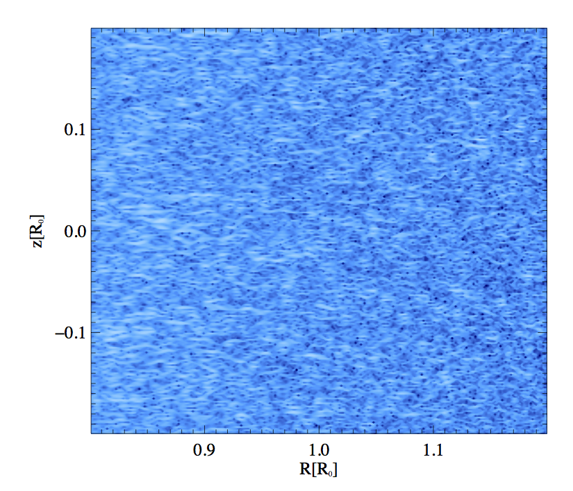
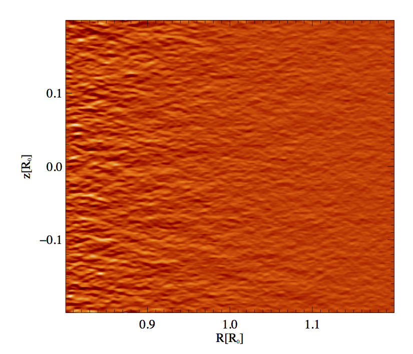
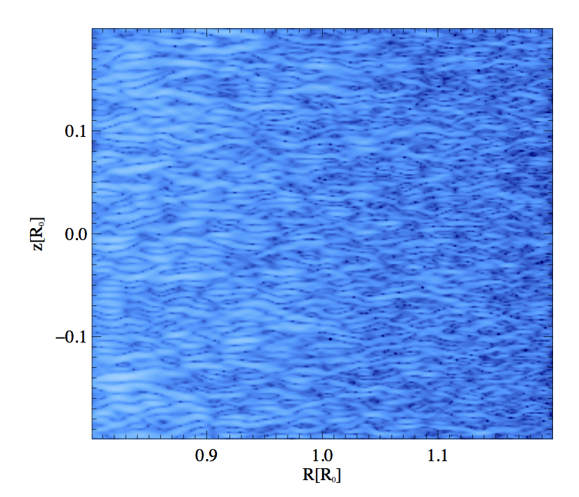
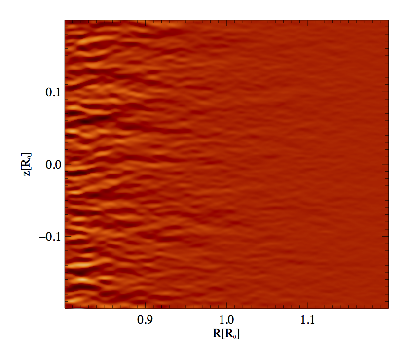
Figure 4: Evolution of the instability for $q=-2;p=-1.32$: From top to bottom at 13 and 65 orbits after initial perturbation. On the left (blue) we plot the absolute value of the velocity in units of the local sound speed and on the right the relative perturbations of the local temperature (red) against the back ground temperature. The colors are scaled to the actual maximum value for better contrast: $v_{\rm max}(t=13,65)/c_{s}=0.0013,0.015;dT_{\rm max}(t=13,65)/T_{0}=0.00012,0.0011$.

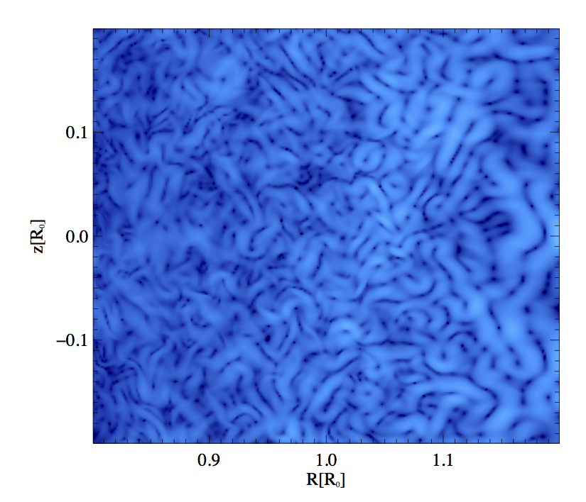
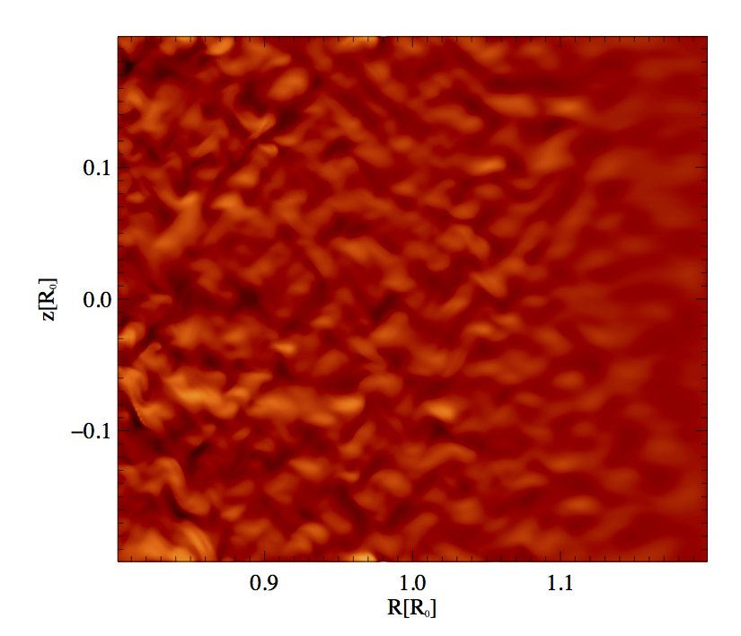
Figure 5: Evolution of the instability for $q=-2;p=-1.32$: 130 orbits after initial perturbation. Colors same as Fig. 4: $v_{\rm max}(t=130)/c_{s}=0.045;dT_{\rm max}(t=130)/T_{0}=0.0036$.

In Figs. 4 and 5 we show three snapshots of the evolution of the instability for the most unstable case $q=-2;p=-1.32;\gamma\Omega\tau=1$. One taken at 13 orbits after the perturbation one after 65 and one after 130 orbits (from top to bottom). On the left we plot the absolute value of the velocity in units of the local sound speed and on the right the relative perturbations of the local temperature against the mean back ground temperature. The density fluctuations have generally the same amplitude as the temperature fluctuations, whereas the measured pressure fluctuations are an order of magnitude smaller than the adiabatic pressure fluctuations corresponding to the density fluctuations. This observation is an a posteriori verification of our quasi-hydrostatic approach. The initial perturbations grow both in amplitude as well as in spatial extent. Test simulations without thermal relaxation or without unstable radial stratification did not show any growth.

References

- Andrews et al. (2010) Andrews, S. M., Wilner, D. J., Hughes, A. M., Qi, C., Dullemond, C. P. 2010. Protoplanetary Disk Structures in Ophiuchus. II. Extension to Fainter Sources. The Astrophysical Journal 723, 1241
- Bai (2011) Bai, X.-N. 2011, ApJ, 739, 50
- Balbus & Hawley (1991) Balbus, S. A., & Hawley, J. F. 1991, ApJ, 376, 214
- Bell et al. (1995) Bell, K. R., Lin, D. N. C., Hartmann, L. W., & Kenyon, S. J. 1995, ApJ, 444, 376
- Bell et al. (1997) Bell, K. R., Cassen, P. M., Klahr, H. H., & Henning, T. 1997, ApJ, 486, 372
- Cox (1980) Cox, J. P. 1980, Research supported by the National Science Foundation Princeton, NJ, Princeton University Press, 1980. 393 p.,
- Eddington (1926) Eddington, A. S. 1926, The Internal Constitution of the Stars, Cambridge: Cambridge University Press, 1926. ISBN 9780521337083.,
- D’Alessio et al. (2005) D’Alessio, P., Calvet, N., & Woolum, D. S. 2005, Chondrites and the Protoplanetary Disk, 341, 353
- Fricke (1968) Fricke, K. 1968, ZAp, 68, 317
- Gammie (1996) Gammie, C. F. 1996, ApJ, 457, 355
- Goldreich & Schubert (1967) Goldreich, P., & Schubert, G. 1967, ApJ, 150, 571
- Kim & Ostriker (2000) Kim, W.-T., & Ostriker, E. C. 2000, ApJ, 540, 372
- Klahr et al. (1999) Klahr, H. H., Henning, T., & Kley, W. 1999, ApJ, 514, 325
- Klahr & Bodenheimer (2000) Klahr, H., & Bodenheimer, P. 2000, Disks, Planetesimals, and Planets, 219, 63
- Klahr & Bodenheimer (2003) Klahr, H. H., & Bodenheimer, P. 2003, ApJ, 582, 869
- Klahr (2004) Klahr, H. 2004, ApJ, 606, 1070
- Klahr et al. (2013) Klahr, H., Raettig, N., & Lyra, W. 2013, European Physical Journal Web of Conferences, 46, 4001
- Kley et al. (2009) Kley, W., Bitsch, B., & Klahr, H. 2009, A&A, 506, 971
- Lesur & Papaloizou (2010) Lesur, G., & Papaloizou, J. C. B. 2010, A&A, 513, A60
- Lyra & Klahr (2011) Lyra, W., & Klahr, H. 2011, A&A, 527, A138
- Marcus et al. (2013) Marcus, P. S., Pei, S., Jiang, C.-H., & Hassanzadeh, P. 2013, Physical Review Letters, 111, 084501
- Miller & Stone (2000) Miller, K. A., & Stone, J. M. 2000, ApJ, 534, 398
- Nelson et al. (2013) Nelson, R. P., Gressel, O., & Umurhan, O. M. 2013, MNRAS, 435, 2610
- Perez-Becker & Chiang (2011) Perez-Becker, D., & Chiang, E. 2011, ApJ, 727, 2
- Petersen et al. (2007) Petersen, M. R., Julien, K., & Stewart, G. R. 2007, ApJ, 658, 1236
- Raettig et al. (2013) Raettig, N., Lyra, W., & Klahr, H. 2013, ApJ, 765, 115
- Shakura & Sunyaev (1973) Shakura, N. I., & Sunyaev, R. A. 1973, A&A, 24, 337
- Turner et al. (2010) Turner, N. J., Carballido, A., & Sano, T. 2010, ApJ, 708, 188
- Rüdiger et al. (2002) Rüdiger, G., Arlt, R., & Shalybkov, D. 2002, A&A, 391, 781
- Velikhov (1959) Velikhov, E. P., 1959, Sov. Phys. JETP, vol. 9 (1959), pp. 995 998 (in Russ.).