The matching problem has no fully-polynomial size
linear programming relaxation schemes

Abstract

The groundbreaking work of Rothvoß (2014) established that every linear program expressing the matching polytope has an exponential number of inequalities (formally, the matching polytope has exponential extension complexity). We generalize this result by deriving strong bounds on the LP inapproximability of the matching problem: for fixed $0<\varepsilon<1$, every $(1-\varepsilon/n)$-approximating LP requires an exponential number of inequalities, where $n$ is the number of vertices. This is sharp given the well-known $\rho$-approximation of size $O(\binom{n}{1/(1-\rho)})$ provided by the odd-sets of size up to $1/(1-\rho)$. Thus matching is the first problem in $P$, which does not admit a fully polynomial-size LP relaxation scheme (the LP equivalent of an FPTAS), which provides a sharp separation from the polynomial-size LP relaxation scheme obtained e.g., via constant-sized odd-sets mentioned above.

Analyzing the size of LP formulations is equivalent to examining the nonnegative rank of matrices. We study the nonnegative rank via an information-theoretic approach, and while it reuses key ideas from Rothvoß (2014), the main lower bounding technique is different: we employ the information-theoretic notion of common information as introduced in Wyner (1975) and used for studying LP formulations in Braun and Pokutta (2013). This allows us to analyze the nonnegative rank of perturbations of slack matrices, e.g., approximations of the matching polytope. It turns out that the high extension complexity for the matching problem stems from the same source of hardness as in the case of the correlation polytope: a direct sum structure.

1 Introduction

In recent years, there has been a significant interest in understanding the expressive power of linear programs. The motivating question is which polytopes or combinatorial optimization problems can be expressed as linear programs with a small number of inequalities. The theory of extended formulations studies this question and the measure of interest is the extension complexity which is the size of the smallest linear programming formulation (in terms of the number of inequalities). This notion of complexity is independent of P vs. NP and is characterized by nonnegative matrix factorizations. We will analyze this factorization problem for the all-important matching problem using information theory.

Most of the recent progress in extended formulations is ultimately rooted in Yannakakis (1988, 1991) seminal paper ruling out symmetric linear programs with a polynomial number of inequalities for the TSP polytope and the matching polytope. It was the innocent question whether the same still holds true when the symmetry assumption is removed that spurred a significant body of work (see Section 1.1 below). Yannakakis’s question was answered in the affirmative in Fiorini et al. (2012b) for the TSP polytope via the correlation polytope, and in Rothvoß (2014) for the matching polytope.

The fact that the matching problem has high extension complexity raises some fundamental questions. After all, matching can be solved in polynomial time. Two key questions are (1) how well we can approximate the matching problem via a linear program (2) what commonality the correlation polytope and the matching problem possess so that both require an exponential number of inequalities. In this work, we answer both of these questions.

We generalize the results in Rothvoß (2014) to show in Theorem 3.1 that the matching problem cannot be approximated within a factor of $1-\Theta(1/n)$ by a linear program with a polynomial number of inequalities. Thus, the matching problem does not admit a fully polynomial-size linear programming relaxation scheme (FPSRS), the linear programming equivalent of an FPTAS, i.e., it cannot be $(1-\varepsilon)$-approximated with a linear program of size $\operatorname{poly}(n,1/\varepsilon)$. This complements the folklore polynomial-sized $(1-1/k)$-approximate linear programming formulation for the matching problem (see Example 2.6), establishing a threshold of $\Theta(1/n)$ between polynomial-size approximability and exponential inapproximability.

Further, our approach is based on a direct information-theoretic argument extending the techniques developed in Braun and Pokutta (2013). This proof exhibits key commonalities with the one for the correlation polytope, revealing that the reason for high complexity of both, the matching problem and the correlation polytope, is an (almost identical) direct sum structure contained in both problems.

1.1 History of extended formulations

We will now provide a brief overview of extended formulations. As mentioned before, the interest in extended formulation was initiated by the question of Yannakakis whether the TSP polytope and the matching polytope have (asymmetric) linear programs with a polynomial number of inequalities. In Kaibel et al. (2010) it was shown that the symmetry actually can make a significant difference for the size of extended formulations. The authors studied the $\ell$-matching polytope (polytope of all matchings with exactly $\ell$ edges), closely related to Yannakakis’s work prompting the question whether every 0/1 polytope has an efficient polyhedral lift (note that this is independent of P vs. NP as we disregard encoding length). This question was answered in the negative in Rothvoß (2012), establishing the existence of 0/1 polytopes requiring an exponential number of inequalities in any of their formulations, and it was recently extended to the case of SDP-based extended formulations in Briët et al. (2013). The same technique was used in Fiorini et al. (2012c) to derive lower bounds on the extension complexity of polygons in the plane, which are of prototypical importance for many related applications; the analogous results for the SDP case have been obtained in Briët et al. (2013).

Shortly after Rothvoß’s result it was shown in Fiorini et al. (2012b) that the first half of Yannakakis’s question is in the affirmative: the TSP polytope requires an exponential number of linear inequalities in any linear programming formulation, irrespective of P vs. NP. In fact, it was shown that the correlation polytope (or equivalently the cut polytope) has extension complexity $2^{\Omega(n)}$ where $n$ is the length of the bit strings, and the stable set polytope (over a certain family of graphs) as well as the TSP polytope have extension complexity $2^{\Omega(n^{1/2})}$ where $n$ is the number of nodes in the graph. In Braun et al. (2012) the result for the correlation polytope was generalized to the approximate case, showing that the CLIQUE polytope, also called the correlation polytope, cannot be approximated with a polynomial-size linear program better than $n^{1/2-\varepsilon}$, which was subsequently improved in Braverman and Moitra (2012) to $n^{1-\varepsilon}$ matching Håstad’s celebrated inapproximability result for the CLIQUE problem (see Håstad (1999)). In Braun and Pokutta (2013) the results for the CLIQUE polytope was further improved to average-case type results via a general information-theoretic framework to lower bound the nonnegative rank of matrices. In Braun et al. (2014a) these average-case arguments were used to show that the average-case (as well as high-probability) extension complexity of the stable-set problem is high. Very recently in Lee et al. (2014) strong explicit lower bounds on the semidefinite extension complexity of the correlation polytope (and many other problems) have been obtained.

Additional bounds for various polytopes including the knapsack polytope have been established in Pokutta and Van Vyve (2013) and Avis and Tiwary (2013) using the reduction mechanism outlined in Fiorini et al. (2012b). Besides CLIQUE and stable set, there are only few results on approximability of problems by linear programs. For any fixed $\varepsilon>0$, a polynomial-sized linear program giving a $(1-\varepsilon)$-approximation of the knapsack problem has been provided in Bienstock (2008). An exponential lower bound on the approximate polyhedral complexity of the metric capacitated facility location problem was established in Kolliopoulos and Moysoglou (2013), however only in the original space; extended formulations were not considered.

Recently, it has been observed that the same techniques (and in fact essentially identical proofs) can be used to obtain results on the size of formulations independent of the actual encoding of the problem as polytope. This generalization was first observed for uniform formulations in Chan et al. (2013), extended to general (potentially non-uniform) problems in Braun et al. (2014a) for analyzing the average case complexity of the stable set problem, and fully generalized to affine functions allowing for approximations and reductions in Braun et al. (2014b) providing inapproximability results for various problems, such as e.g., vertex cover. All these versions are extensions of the initial approach to approximations via polyhedral pairs (see Braun et al. (2012); Pashkovich (2012)).

The main tool for lower bounds is Yannakakis’s celebrated Factorization Theorem stating that the extension complexity of a polytope is equal to the nonnegative rank of any of its slack matrices, which has been extended to the approaches mentioned above. Combinatorial as well as communication based lower bounds for the nonnegative rank have been explored in Faenza et al. (2012); Fiorini et al. (2012a). At the core of all of the above super-polynomial lower bounds on the extension complexity is the all-important UDISJ problem whose partial matrix appears as a pattern in the slack matrix of these problems. The current best lower bound on the nonnegative rank of the UDISJ matrix is established in Kaibel and Weltge (2013) by a remarkably short combinatorial argument.

Two notable exceptions not using UDISJ are Chan et al. (2013); Lee et al. (2014), mentioned above adapting Sherali-Adams and Lasserre separators to obtain lower bounds. Another exception is the very recent result of Rothvoß (2014), which finally answers the second half of Yannakakis’s question, showing that the matching polytope has exponential extension complexity. The proof is based on Razborov’s technique (see Razborov (1992)), and provides the second base matrix with linear rank but exponential nonnegative rank, namely, the slack matrix of the matching problem.

1.2 Related work

We recall the works whose methodology is closely related to ours. The most closely related one is Braun and Pokutta (2013) providing a general information-theoretic framework for lower bounding the extension complexity of polytopes in terms of information, motivated by Braverman et al. (2012) as well as Jain et al. (2013). A dual information-theoretic approach, similar to the one for the fractional rectangle covering number (see e.g., Karchmer et al. (1995)) has been explored in Braun et al. (2013), however, we will stick to the primal approach here, dealing directly with distributions over potential rank-1 matrices. The cornerstone of our framework is the notion of common information introduced by Wyner (1975) for (a completely unrelated) use in information theory. For estimating information, Braun and Pokutta (2013) used Hellinger distance inspired by Bar-Yossef et al. (2004), however here it is more effective to employ Pinsker’s inequality. The model of approximate linear programs is the same as in Braun et al. (2014b) based on Chan et al. (2013); see also Braun et al. (2014a).

1.3 Contribution

Our main result is Theorem 3.1 proving inapproximability of the matching polytope, providing the following three main contributions. We use the term formulation complexity for the complexity of linear programming formulations (again measured in the number of required linear inequalities), as introduced in Braun et al. (2014b). This notion is a natural generalization of extension complexity, not requiring a polytope encoding for optimization problems.

1. Polyhedral inapproximability of the matching problem: As mentioned above, the matching problem can be solved in polynomial time, even though its formulation complexity is exponential. However, it can be $(1-\varepsilon)$-approximated by a linear program of polynomial size for an fixed $\varepsilon>0$, i.e., it admits a polynomial-size linear programming relaxation scheme (PSRS), which is the linear programming equivalent of a PTAS. As a consequence, an important and natural question is whether one can even go a step further and find a linear program of size $\operatorname{poly}(n,1/\varepsilon)$ approximating the matching polytope within a factor of $1-\varepsilon$, i.e., whether it admits a fully polynomial-size linear programming relaxation scheme (FPSRS); the linear programming equivalent of an FPTAS. We resolve this question in the negative, showing that the formulation complexity and (classical) computational complexity are very different notions. The non-existence of an FPSRS for matching can be also interpreted as an indicator that matching might be especially hard from a linear programming point of view, similar to the notion of strong NP-hardness which also precludes the existence of an FPTAS (in most cases) in the computational complexity setup.

2. Information-theoretic proof: We provide an information-theoretic proof for the lower bound on the linear programming complexity of the matching problem and its approximations. The proof is based on an extension of the framework in Braun and Pokutta (2013). By arguing directly via the distribution of potential factorizations, rather than considering single rank-1 factors or rectangles as typically required by Razborov’s method, the setup can be considerably simplified and the information-theoretic framework naturally lends itself to approximations. We obtain a simple and short proof that provides additional insight into the structure of matchings and their linear programming hardness.

3. High complexity implied by direct sum structure: The information-theoretic approach is well suited for proving exponential lower bounds by partitioning the structure $P$ into copies of a fixed-size substructures $P_{0}$, and applying a direct sum argument to show

   $$\log\operatorname{fc}(P)\geq\Theta(n)\cdot\log\operatorname{fc}(P_{0}),$$

   where $\operatorname{fc}(Q)$ denotes the formulation complexity of $Q$ and the bound on $\operatorname{fc}(P_{0})$ is non-trivial. This was already used for the correlation polytope in Braun and Pokutta (2013), and we show that the matching polytope exhibits a similar direct sum structure. The partition we use is a simplified variant of the one in Rothvoß (2014), however it is still slightly more involved than the one for the correlation polytope due to additional structure we need to consider.

In the above direct sum framework, the difficulty arises from actually having an information-theoretic quantity in place of $\log\operatorname{fc}(P_{0})$, which is used to make the direct sum argument work in first place. Thus a positive constant lower bound is not immediate, in particular when considering approximations.

The authors believe that the presented approach can be also used to obtain linear programming inapproximability results for a variety of other problems.

1.4 Outline

We start with preliminaries in Section 2, introducing necessary notions and notations from information theory in Section 2.1 as well as providing a recap of the theory of (approximate) LP formulations in Section 2.2. In Section 2.3 we provide the connection between common information and nonnegative rank, which is subsequently extended to provide bounds for the matching problem in Section 3. We choose notations mostly consistent with Rothvoß (2014) for easy relation of both approaches.

2 Preliminaries

We use $[k]\coloneqq\left\{1,\dots,k\right\}$ as a short-hand. Let $\log$ denote the logarithm to base $2$. We will denote random variables by bold capital letters such as $\mathbf{A}$ to avoid confusion with sets that will also be denoted by capital letters. Events will be denoted by capital script letters such as $\mathscr{E}$ when not written out, but conditions will be denoted by script bold letters such as $\boldsymbol{\mathscr{Z}}$ in conditional probabilities and other conditional quantities: conditions can be events, random variables, or combinations of both types. We use $\perp$ to indicate independence: e.g., $\mathbf{A}\perp\mathbf{B}$.

2.1 Information-theoretic basics

We briefly recall standard basic notions from information theory in this section and we refer the reader to Cover and Thomas (2006) for more details and as an excellent introduction. Information is measured in bits, as is standard for discrete random variables.

We will now recall the notion of mutual information which is at the core of our arguments. The mutual information of two discrete random variables $\mathbf{A},\mathbf{B}$ is defined as

$$\mathbb{I}\left[\mathbf{A};\mathbf{B}\right]\coloneqq\sum_{\begin{subarray}{c}a\in\operatorname{range}(\mathbf{A})\\ b\in\operatorname{range}(\mathbf{B})\end{subarray}}\operatorname{\mathbb{P}}\left[\mathbf{A}=a,\mathbf{B}=b\right]\log\frac{\operatorname{\mathbb{P}}\left[\mathbf{A}=a,\mathbf{B}=b\right]}{\operatorname{\mathbb{P}}\left[\mathbf{A}=a\right]\cdot\operatorname{\mathbb{P}}\left[\mathbf{B}=b\right]}.$$

It captures how much information about $\mathbf{A}$ is leaked by considering $\mathbf{B}$; and vice versa: mutual information is symmetric. We will often have $\mathbf{A}$ and $\mathbf{B}$ being a collection of random variables. We use a comma to separate the components of $\mathbf{A}$ or $\mathbf{B}$, and a semicolon to separate $\mathbf{A}$ and $\mathbf{B}$ themselves, e.g., $\mathbb{I}\left[\mathbf{A}_{1},\mathbf{A}_{2};\mathbf{B}\right]=\mathbb{I}\left[(\mathbf{A}_{1},\mathbf{A}_{2});\mathbf{B}\right]$. We can naturally extend mutual information to conditional mutual information

$$\mathbb{I}\left[\mathbf{A};\mathbf{B}\,\middle|\,\mathbf{C},\mathscr{E}\right]\coloneqq\operatorname{\mathbb{E}}_{\mathbf{C}\mid\mathscr{E}}\left[\mathbb{I}\left[(\mathbf{A}\mid\mathbf{C},\mathscr{E});(\mathbf{B}\mid\mathbf{C},\mathscr{E})\right]\right]$$

by using the respective conditional distributions, where $\mathbf{C}$ is a random variable and $\mathscr{E}$ is an event. Note that the expectation is implicitly taken over random variables in the condition.

We shall use the following bounds on mutual information. An obvious upper bound is

$$\mathbb{I}\left[\mathbf{A};\mathbf{B}\,\middle|\,\boldsymbol{\mathscr{Z}}\right]\leq\log\left|\operatorname{range}(A)\right|,$$

which provides the lower bound on the logarithm of the nonnegative rank in Lemma 2.11.

Exponential lower bounds of the nonnegative rank will be obtained via the direct sum property, which states that for mutually independent random variables $\mathbf{A_{1}},\dotsc,\mathbf{A_{n}}$ given a condition $\boldsymbol{\mathscr{Z}}$ we have

$$\mathbb{I}\left[\mathbf{A_{1}},\dotsc,\mathbf{A_{n}};\mathbf{B}\,\middle|\,\boldsymbol{\mathscr{Z}}\right]\geq\sum_{i\in[n]}\mathbb{I}\left[\mathbf{A_{i}};\mathbf{B}\,\middle|\,\boldsymbol{\mathscr{Z}}\right].$$

In order to lower bound each summand we will use a divergence measure. The relative entropy or Kullback–Leibler divergence measures the difference of two probability distributions. It is always nonnegative, but it is neither symmetric, nor does it satisfy the triangle inequality. For simplicity we only define it for random variables.

Definition 2.1 (Relative entropy).

Let $\mathbf{X},\mathbf{Y}$ be discrete random variables on the same domain. Relative entropy of $\mathbf{X}$ and $\mathbf{Y}$ is

$$\operatorname{\mathbb{D}}\left(\mathbf{X}\,\middle\|\,\mathbf{Y}\right)=\sum_{x\in\operatorname{range}(\mathbf{X})}\operatorname{\mathbb{P}}\left[\mathbf{X}=x\right]\cdot\log\frac{\operatorname{\mathbb{P}}\left[\mathbf{X}=x\right]}{\operatorname{\mathbb{P}}\left[\mathbf{Y}=x\right]}.$$

Here $0\log(0/q)=0$ and $p\log(p/0)=+\infty$ for $p>0$ by convention.

Relative entropy is related to mutual information via the following identity:

$$\mathbb{I}\left[\mathbf{X};\mathbf{Y}\right]=\operatorname{\mathbb{E}}_{\mathbf{Y}}\left[\operatorname{\mathbb{D}}\left(\mathbf{X}\mid\mathbf{Y}\,\middle\|\,\mathbf{X}\right)\right],$$

i.e., mutual information is the expectation of the deviation over $\mathbf{Y}$. Pinsker’s inequality provides a convenient lower bound on the relative entropy (see e.g., (Cover and Thomas, 2006, Lemma 11.6.1)).

Lemma 2.2 (Pinsker’s inequality).

Let $\mathbf{X},\mathbf{Y}$ be discrete random variables with identical domains. Then

$$\operatorname{\mathbb{D}}\left(\mathbf{X}\,\middle\|\,\mathbf{Y}\right)\geq 2(\log e)\left(\max_{\mathscr{E}\colon\textup{ event}}\left|\operatorname{\mathbb{P}}\left[\mathscr{E}(\mathbf{X})\right]-\operatorname{\mathbb{P}}\left[\mathscr{E}(\mathbf{Y})\right]\right|\right)^{2}.$$

The quantity $\max_{\mathscr{E}:\textup{ event}}\left|\operatorname{\mathbb{P}}\left[\mathscr{E}(\mathbf{X})\right]-\operatorname{\mathbb{P}}\left[\mathscr{E}(\mathbf{Y})\right]\right|$ is called the total variation distance between $\mathbf{X}$ and $\mathbf{Y}$, which is the maximal difference of probabilities the distributions of $\mathbf{X}$ and $\mathbf{Y}$ assign to the same event. For mutual information, via Pinsker’s inequality we obtain the lower bound

$$\mathbb{I}\left[\mathbf{X};\mathbf{Y}\right]\geq 2(\log e)\cdot\operatorname{\mathbb{E}}_{\mathbf{Y}}\left[\max_{\mathscr{E}:\textup{ event}}\left|\operatorname{\mathbb{P}}\left[\mathscr{E}(\mathbf{X})\right]-\operatorname{\mathbb{P}}\left[\mathscr{E}(\mathbf{X})\,\middle|\,\mathbf{Y}\right]\right|^{2}\right].$$

2.2 Approximations via linear programs

We will now recall the framework of linear programming formulations from Braun et al. (2014b), subsuming previous approaches via polyhedral pairs, but with the advantage of requiring no linear encoding for the problem statement. It also includes a reduction to matrix factorizations, reducing bounds on the size of linear programming formulations to bounds of nonnegative rank of matrices.

We refer the interested reader to the excellent surveys Conforti et al. (2010) and Kaibel (2011) as well as Pashkovich (2012); Braun et al. (2012) for the approximate extended formulation framework via polyhedral pairs.

We are interested in questions of the following type:

How hard is it to approximate a maximization problem $\operatorname{\mathcal{P}}$ within
a factor of $\rho$ via a linear programming formulation?

One could ask the same question for minimization problems, and the framework below also applies to them, but for simplicity, here we restrict the exposition to maximization problems only.

We start by making the notion of a maximization problem precise. A maximization problem $\operatorname{\mathcal{P}}=(\mathcal{S},\mathcal{F})$ consists of a set of feasible solutions $\mathcal{S}$ and a set of objective functions $\mathcal{F}$ defined on $\mathcal{S}$. The aim is to approximate the maximum value of every objective function in $\mathcal{F}$ over $\mathcal{S}$. An approximation problem $\operatorname{\mathcal{P}}^{*}=(\operatorname{\mathcal{P}},\mathcal{F}^{*})$ is a maximization problem $\operatorname{\mathcal{P}}$ together with a family $\mathcal{F}^{*}=\left\{f^{*}\,\middle|\,f\in\mathcal{F}\right\}$ of numbers called approximation guarantees satisfying $\max f\leq f^{*}$. An algorithm solves $\operatorname{\mathcal{P}}^{*}$ if it computes for every $f\in\mathcal{F}$ an approximate value $\widehat{f}$ satisfying $\max f\leq\widehat{f}\leq f^{*}$. This is a formalization of the traditional notion of approximation algorithms. For example setting $f^{*}=\max f$ we compute the exact maximum values. Often the objective functions are nonnegative, and one wants to approximate the maximum within a factor $0<\rho<1$. Recall that an approximation factor $\rho$ for an approximation algorithm means that the algorithm computes a solution $s$ with $f(s)\geq\rho\max f$, and in order to be compatible with this model we use the equivalent outer approximation in our model, i.e., we choose $f^{*}=\max f/\rho$.

We will consider the matching problem with the following specification.

Definition 2.3 (Matching problem).

The matching problem Matching($n$) has as feasible solutions all matchings $M$ of the complete graph $K_{n}$ on $[n]$. The objective functions $f_{G}$ are indexed by all graphs $G$ with $V(G)\subseteq[n]$ with function values

$$f_{G}(M)\coloneqq\left|M\cap E(G)\right|.$$

Note that $M\cap E(G)$ is a matching of $G$, and a matching $M$ of $G$ is also a matching of $K_{n}$. In particular, $\max f_{G}=\mu(G)$ is the matching number of $G$.

2.2.1 LP formulation

To complete the framework, we will now define linear programming formulations. Given an approximation problem $\operatorname{\mathcal{P}}^{*}=(\operatorname{\mathcal{P}},\mathcal{F}^{*})$ with $\operatorname{\mathcal{P}}=(\mathcal{S},\mathcal{F})$ as above, an LP formulation of $\operatorname{\mathcal{P}}^{*}$ consists of

1. a linear program $Ax\leq b$ with variables $x\in\mathbb{R}^{d}$ for some $d$;

2. a realization $x^{s}\in\mathbb{R}^{d}$ for every feasible solution $s\in\mathcal{S}$ satisfying $Ax^{s}\leq b$;

3. a realization $w^{f}\colon\mathbb{R}^{d}\to\mathbb{R}$ for every objective function $f\in\mathcal{F}$ as an affine map satisfying $w^{f}(x^{s})=f(s)$,

and we require that the linear program maximizing $w^{f}(x)$ subject to $Ax\leq b$ yields a solution within the approximation guarantee $f^{*}$, i.e., $\widehat{f}\coloneqq\max_{x:Ax\leq b}w^{f}(x)\leq f^{*}$.

The size of an LP formulation is the number of inequalities in $Ax\leq b$ and the formulation complexity $\operatorname{fc}(\operatorname{\mathcal{P}}^{*})$ of $\operatorname{\mathcal{P}}^{*}$ is the minimum size of its LP formulations. When approximation guarantees are given via an approximation factor $0<\rho\leq 1$, i.e., $f^{*}=\max f/\rho$, we shall write $\operatorname{fc}(\operatorname{\mathcal{P}},\rho)$ for the formulation complexity.

The matching polytope provides an LP formulation of the exact matching problem:

Example 2.4 (The matching polytope as formulation of the matching problem).

The matching polytope $P_{M}(n)$ is defined as the convex hull of the characteristic vectors $\chi_{M}$ of all matchings $M$:

$$P_{M}(n)\coloneqq\operatorname{conv}\left(\chi_{M}\in\mathbb{R}^{\binom{n}{2}}\,\middle|\,M\text{ is a matching in }K_{n}\right).$$

Recall from Edmonds (1965) that the matching polytope $P_{PM}(n)$ is the solution set of the linear program

$$x(\delta(v)) \leq 1 v \in[n],$$

$$x(E[U]) \leq\frac{\left|U\right|-1}{2} U \subseteq[n],\left|U\right|\text{ odd},$$

$$x \geq 0.$$

Here and below for a vertex set $U\subseteq[n]$, let $E[U]$ denote the set of edges of the graph $K_{n}$ contained in $U$, and let $\delta(U)$ denote the set of edges with one endpoint in $U$ and one in its complement; we use $\delta(v)\coloneqq\left|\delta(\left\{v\right\})\right|$ to denote the degree of $v\in[n]$. Finally, $x(E)\coloneqq\sum_{\{i,j\}\in E}x_{i,j}$ denotes the sum of the coordinates of $x$ from an arbitrary edge set $E$.

This linear program provides an LP formulation for Matching($n$) with realizations $x^{M}=\chi_{M}$ for matchings $M$ and the linear functions $w^{f_{G}}(x)=x(E(G))$ for objective functions $f_{G}$. Observe that most of the inequalities have the form $w^{f_{K_{U}}}(x)\leq\max f_{K_{U}}$, which will be useful later.

2.2.2 Polynomial-size linear programming relaxation schemes

We will also examine the trade-off between approximation factor and size. The following two notions are the linear programming equivalents of PTAS and FPTAS.

Definition 2.5 ((Fully) polynomial-size linear programming relaxation scheme).

Let $\operatorname{\mathcal{P}}_{n}$ with $n\in\mathbb{N}$ be a family of maximization problems. The family $\{\operatorname{\mathcal{P}}_{n}\}_{n\in\mathbb{N}}$ admits a

1. polynomial-size linear programming relaxation scheme (PSRS) if for every fixed $\varepsilon>0$ there is an LP formulation of $\operatorname{\mathcal{P}}_{n}$ with approximation factor $1-\varepsilon$, whose size is bounded by a polynomial in $n$, i.e., $\operatorname{fc}(\operatorname{\mathcal{P}}_{n},1-\varepsilon)\leq\operatorname{poly}(n)$.

2. fully polynomial-size linear programming relaxation scheme (FPSRS) if for every $\varepsilon>0$ there is an LP formulation of $\operatorname{\mathcal{P}}_{n}$ with approximation factor $1-\varepsilon$, whose size is bounded by a polynomial in $n$ and $1/\varepsilon$, i.e., $\operatorname{fc}(\operatorname{\mathcal{P}}_{n},1-\varepsilon)\leq\operatorname{poly}(n,1/\varepsilon)$ for every $\varepsilon>0$ and $n$.

Thus both PSRS and FPSRS require a polynomial $p$ with $\operatorname{fc}(\operatorname{\mathcal{P}}_{n},1-\varepsilon)\leq p(n)$. The difference between PSRSs and FPSRSs is that an FPSRS requires $p$ to depend polynomially on $1/\varepsilon$ as well, whereas for a PSRS the polynomial $p$ is allowed to depend arbitrarily on $1/\varepsilon$.

For example, it is known that the maximum knapsack problem admits a PSRS as shown in Bienstock (2008), however it is not known whether it also admits an FPSRS. The matching problem has the following folklore PSRS:

Example 2.6 (PSRS for matching).

We use the standard realization of the matching problem via the matching polytope $P_{M}(n)$, i.e., represent matchings by their characteristic vectors. We claim that the standard realization with the following linear program is an LP formulation of size $O(n^{1/(1-\rho)})$ for the matching problem with approximation factor $\rho$, for $0<\rho<1$.

$$x(\delta(v)) \leq 1 \forall v \in[n]$$

$$x(E[U]) \leq\frac{\left|U\right|-1}{2\rho} \forall U \subseteq[n],\left|U\right|\text{ odd},\left|U\right|<\frac{1}{1-\rho}$$

$$x \geq 0.$$

Let $K_{n}$ be the polytope defined by these inequalities. For the claim, it is enough to prove $P_{M}(n)\subseteq K_{n}\subseteq\rho^{-1}P_{M}(n)$. The first inequality is obvious, and for the second one, we need to prove that for every $x\in K_{n}$ we have $x(E[U])\leq\frac{\left|U\right|-1}{2\rho}$ for $U\subseteq[n]$ odd and $\left|U\right|\geq\frac{1}{1-\rho}$. This inequality follows by summing up the inequalities $x(\delta(v))\leq 1$ for $v\in U$ and using $x\geq 0$:

$$x(E[U])\leq\frac{1}{2}\sum_{v\in U}x(\delta(v))\leq\frac{\left|U\right|}{2}\leq\frac{\left|U\right|-1}{2\rho}.$$

2.2.3 Slack matrix and factorization

The main tool for lower bounding the formulation complexity is via the nonnegative rank of the slack matrix.

Definition 2.7 (Slack matrix).

Given an approximation problem $\operatorname{\mathcal{P}}^{*}=(\operatorname{\mathcal{P}},\mathcal{F}^{*})$ of a maximization problem $\operatorname{\mathcal{P}}=(\mathcal{S},\mathcal{F})$, the slack matrix $S$ of $\operatorname{\mathcal{P}}^{*}$ is the $\mathcal{F}\times\mathcal{S}$ matrix where $S_{f,s}\coloneqq f^{*}-f(s)$ for all $f,s$.

The nonnegative rank $\operatorname{rk_{+}}S$ of a nonnegative matrix $S$ is the smallest nonnegative integer $r$ such that $M=\sum_{i\in[r]}M_{i}$ is a sum of $r$ nonnegative rank-$1$ matrices $M_{i}$. Yannakakis’s factorization theorem identifies extension complexity of a polytope with the nonnegative rank of any of its slack matrices (see Yannakakis (1988, 1991)). The theorem extends naturally to the notion of formulation complexity:

Theorem 2.8 ((Braun et al., 2014b, Theorem 3.3)).

Let $\operatorname{\mathcal{P}}^{*}$ be an approximation problem with slack matrix $S$. Then $-1+\operatorname{rk_{+}}S\leq\operatorname{fc}(\operatorname{\mathcal{P}}^{*})\leq\operatorname{rk_{+}}S$.

Thus, for a lower bound on formulation complexity, it suffices to lower bound the nonnegative rank of the slack matrix of the problem of interest. We refer the interested reader also to Pashkovich (2012); Braun et al. (2012) for a similar theorem using the classical polyhedral pairs approach. Actually, formulation complexity is equal to a modified version of nonnegative rank, showing that it is completely determined by the slack matrix. However, for our purposes here it will be sufficient to consider the nonnegative rank of the slack matrix.

We will establish the non-existence of an FPSRS for the matching problem by providing a lower bound for $\operatorname{fc}(\textnormal{{Matching($n$)}},\rho)$ for suitably chosen $\rho$. For this, we consider the approximation problem $\textnormal{{Matching($n$)}}^{*}_{\varepsilon}$ with $0<\varepsilon\leq 1$, where the underlying maximization problem is the subproblem of Matching($n$) with objective functions restricted to the $f_{U}$ for complete graphs $K_{U}$ for odd sets $U\subseteq[n]$ and feasible solutions only the perfect matchings $M$. In particular, we assume $n$ is even. The intuition is that every maximal matching $M$ of a graph $G$ arises as the restriction of any perfect matching $M^{\prime}$, obtained by extending $M$, and hence this restriction does not alter the maximum value of functions. The restriction to complete graphs on odd sets is motivated by the LP formulation given by the matching polytope, where the overwhelming majority of facets correspond to such graphs.

We choose approximation guarantees slightly weaker than coming from the approximation factor $1-\varepsilon/(n-1)$, in order to simplify the later analysis:

$$f^{*}_{K_{U}}\coloneqq\frac{\left|U\right|-1+\varepsilon}{2}\geq\frac{\left|U\right|-1}{2(1-\varepsilon/(n-1))},$$

where the inequality is equivalent to $\left|U\right|\leq n-\varepsilon$, which clearly holds. With this choice the slack entries depend only on the number of crossing edges:

$$S_{M,U}^{+\varepsilon}\coloneqq\frac{\left|U\right|-1+\varepsilon}{2}-\left|E[U]\cap M\right|=\frac{\left|\delta(U)\cap M\right|-1+\varepsilon}{2},$$

whereas for an approximation factor $\rho$, the slack entries would also depend on the size of $U$:

$$S_{M,U}^{\rho}\coloneqq\frac{\left|U\right|-1}{2\rho}-\left|E[U]\cap M\right|=\frac{1}{2}\left(\left|\delta(U)\cap M\right|-1+\frac{1-\rho}{\rho}(\left|U\right|-1)\right),$$

which would complicate the analysis.

2.3 Lower bounds on the nonnegative rank via common information

We further extend the common information-based framework that was introduced in Braun and Pokutta (2013) and expanded in Braun et al. (2013). The underlying approach is based on the sampling framework introduced in Braverman and Moitra (2012) and implicitly related to previous lower bounding techniques given in Bar-Yossef et al. (2004). We bound the log nonnegative rank from below by common information, an information-theoretic quantity that was introduced in Wyner (1975). We recall the basic framework here and apply it to the matching problem in Section 3.

Definition 2.9 (Common information).

Let $\mathbf{A},\mathbf{B}$ be random variables, and $\boldsymbol{\mathscr{Z}}$ be a conditional. The common information of $\mathbf{A},\mathbf{B}$ given $\boldsymbol{\mathscr{Z}}$ is the quantity

$$\mathbb{C}\left[\mathbf{A};\mathbf{B}\,\middle|\,\boldsymbol{\mathscr{Z}}\right]\coloneqq\inf_{\begin{subarray}{c}\mathbf{\Pi}\colon\mathbf{A}\perp\mathbf{B}\mid\mathbf{\Pi}\\ \mathbf{\Pi}\perp\boldsymbol{\mathscr{Z}}\mid\mathbf{A},\mathbf{B}\end{subarray}}\mathbb{I}\left[\mathbf{A},\mathbf{B};\mathbf{\Pi}\,\middle|\,\boldsymbol{\mathscr{Z}}\right],$$ (1)

where the infimum is taken over all random variables $\mathbf{\Pi}$ in all extensions of the probability space, so that

1. $\mathbf{A}$ and $\mathbf{B}$ are conditionally independent given $\mathbf{\Pi}$, and

2. $\boldsymbol{\mathscr{Z}}$ and $\mathbf{\Pi}$ are conditionally independent given $\mathbf{A}$ and $\mathbf{B}$.

We refer to $\mathbf{\Pi}$ as seed whenever it satisfies the above properties.

Note that when the condition includes random variables, expectation should be automatically taken over all of them when computing the mutual information. In particular, common information is not a function of the random variables in its condition.

The conditional independence of $\boldsymbol{\mathscr{Z}}$ and $\mathbf{\Pi}$ is to ensure that no information about $\mathbf{\Pi}$ should be leaked from $\boldsymbol{\mathscr{Z}}$. We will link common information to nonnegative matrices, by reinterpreting the latter as probability distributions over two random variables $\mathbf{A}$ and $\mathbf{B}$.

Definition 2.10 (Induced distribution).

Let $M\in\mathbb{R}_{+}^{m\times n}$ be a nonnegative matrix. The induced distribution on $\mathbf{A},\mathbf{B}$ with $\operatorname{range}(\mathbf{A})=[m]$ and $\operatorname{range}(\mathbf{B})=[n]$ via $M$ is given by

$$\operatorname{\mathbb{P}}\left[\mathbf{A}=a,\mathbf{B}=b\right]=\frac{M(a,b)}{\sum_{x,y}M(x,y)}$$

for every row $a$ and column $b$. Slightly abusing notation, we write $(\mathbf{A},\mathbf{B})\sim M$.

For convenience we define the common information of $M$ conditioned on $\boldsymbol{\mathscr{Z}}$ as

$$\mathbb{C}\left[M\,\middle|\,\boldsymbol{\mathscr{Z}}\right]\coloneqq\mathbb{C}\left[\mathbf{A};\mathbf{B}\,\middle|\,\boldsymbol{\mathscr{Z}}\right],$$ (2)

where $(\mathbf{A},\mathbf{B})\sim M$. It can be shown that common information is a lower bound on the log of the nonnegative rank.

Lemma 2.11 (Braun and Pokutta (2013)).

Every nonnegative factorization of a nonnegative matrix $M$ induces a seed with range of size of the number of summands in the factorization. In particular, $\log\operatorname{rk_{+}}M\geq\mathbb{C}\left[M\,\middle|\,\boldsymbol{\mathscr{Z}}\right]$ for any condition $\boldsymbol{\mathscr{Z}}$.

Even though it is not needed in the sequel, for the sake of completeness, we briefly recall the seed $\mathbf{\Pi}$ arising from a nonnegative matrix factorization $M=\sum_{i\in[r]}u_{i}^{\intercal}v_{i}$ of $M$. We start from a probability space $\Omega$ containing the random row $\mathbf{A}$, the random column $\mathbf{B}$, and possibly other random variables, needed to define $\boldsymbol{\mathscr{Z}}$. Given an outcome of $\Omega$, we choose $\mathbf{\Pi}\in[r]$ with conditional distribution

$$\operatorname{\mathbb{P}}\left[\mathbf{\Pi}=i\,\middle|\,\mathbf{A},\mathbf{B}\right]=\frac{u_{i}(\mathbf{A})\cdot v_{i}(\mathbf{B})}{M_{\mathbf{A},\mathbf{B}}}.$$

This choice ensures the conditional independence requirements to make $\mathbf{\Pi}$ a seed: the independence of $\mathbf{\Pi}$ and $\boldsymbol{\mathscr{Z}}$ given $\mathbf{A},\mathbf{B}$, as well as the independence of $\mathbf{A}$ and $\mathbf{B}$ given $\mathbf{\Pi}$.

Clearly, $r\geq\mathbb{H}\left[\mathbf{\Pi}\right]\geq\mathbb{I}\left[\mathbf{A},\mathbf{B};\mathbf{\Pi}\,\middle|\,\boldsymbol{\mathscr{Z}}\right]$, which by taking infimum leads to $\log\operatorname{rk_{+}}M\geq\mathbb{C}\left[M\,\middle|\,\boldsymbol{\mathscr{Z}}\right]$.

3 Formulation complexity of the matching problem

We will now show how to bound the common information of the slack matrix of the matching problem, which leads to a lower bound on the nonnegative rank of the slack matrix and hence the formulation complexity of the matching problem via Theorem 2.8 and Lemma 2.11.

Theorem 3.1.

Let $0<\varepsilon<1$ be fixed and $n$ even. Then $\operatorname{fc}(\textnormal{{Matching($n$)}}^{*}_{\varepsilon})=2^{\Theta(n)}$. In particular, the formulation complexity of the matching problem with approximation factor $1-\varepsilon/n$ is $\operatorname{fc}(\textnormal{{Matching($n$)}},1-\varepsilon/n)=2^{\Theta(n)}$. Therefore the matching problem does not admit an FPSRS.

Establishing Theorem 3.1 reduces to showing that $\mathbb{C}\left[\mathbf{M};\mathbf{U}\,\middle|\,\boldsymbol{\mathscr{Z}}\right]=\Omega(n)$ for $(\mathbf{M},\mathbf{U})\sim S^{+\varepsilon}$ under a suitable condition $\boldsymbol{\mathscr{Z}}$ via Lemma 2.11 and Theorem 2.8.

3.1 Preparation for the proof: probabilistic setup

We need some preparations to introduce $\boldsymbol{\mathscr{Z}}$. We partition the vertices of $K_{n}$ in a manner similar to but simpler than in Rothvoß (2014), see Figure 1. The purpose is to break up the graph into small chunks, in order to amplify the complexity of the chunks.

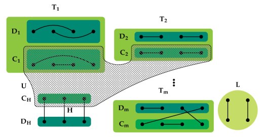
Figure 1: The condition $\mathscr{E}$ together with a partition of $K_{n}$ to reduce formulation complexity to fixed-size small chunks.

First, we choose a $3$-matching $\mathbf{H}$ between two disjoint $3$-element subsets $\mathbf{C_{H}}$ and $\mathbf{D_{H}}$. The intention is to consider only pairs $(\mathbf{M},\mathbf{U})$ with $\mathbf{H}\subseteq\mathbf{M}$ and $\delta(\mathbf{U})\cap\mathbf{M}=\mathbf{H}$, together with $\mathbf{C_{H}}\subseteq\mathbf{U}$ and $\mathbf{U}\cap\mathbf{D_{H}}=\emptyset$. We partition the vertices not covered by $\mathbf{H}$ into equal-sized chunks $\mathbf{T_{1}},\dotsc,\mathbf{T_{m}}$ of even size $2(k-3)$, where $k\geq 7$ is a fixed integer. This might not be possible, and some vertices might be left out, therefore we add a remainder chunk $\mathbf{L}$ (which might be empty) of size $l<2(k-3)$. In particular, $n-6=2(k-3)m+l$. We partition every $\mathbf{T_{i}}$ into a pair of $(k-3)$-element sets $\mathbf{C_{i}},\mathbf{D_{i}}$. We will denote by $\mathbf{T}$ the collection of $\mathbf{C_{1}},\mathbf{D_{1}},\dotsc,\mathbf{C_{m}},\mathbf{D_{m}},\mathbf{C_{H}},\mathbf{D_{H}},\mathbf{L}$. Let $\mathbf{T}$ and $\mathbf{H}$ be jointly uniformly distributed independently of $\mathbf{M},\mathbf{U}$.

Second, we need a collection $\mathbf{N}$ of $m$ mutually independent random fair coins $\mathbf{N_{1}},\dotsc,\mathbf{N_{m}}$, which are also independent of the random variables introduced before. Finally, we introduce the events $\mathscr{E}_{0}$ and $\mathscr{E}$ formalizing the above restrictions of $\mathbf{M},\mathbf{U}$ imposed by $\mathbf{T}$:

$$\mathscr{E}_{0} \coloneqq\left\{\begin{aligned} \mathbf{U}\cap\mathbf{T_{i}}&\in\{\emptyset,\mathbf{C_{i}}\},&\mathbf{C_{H}}\subseteq\mathbf{U}&\subseteq\mathbf{C_{H}}\cup\bigcup_{i\in[m]}\mathbf{C_{i}}\\ \mathbf{H}&\subseteq\mathbf{M},&\mathbf{M}&\subseteq\mathbf{H}\cup E[\mathbf{L}]\cup\bigcup_{i\in[m]}E[\mathbf{T_{i}}]\end{aligned}\right.$$

$$\mathscr{E} \coloneqq\mathscr{E}_{0}\wedge\begin{cases}\mathbf{U}\cap\mathbf{T_{i}}=\emptyset,&\text{if }\mathbf{N_{i}}=0,\\ \delta(\mathbf{C_{i}})\cap\mathbf{M}=\emptyset,&\text{if }\mathbf{N_{i}}=1.\end{cases}$$

In particular, given $\mathscr{E}_{0}$ we have $\mathbf{L}\cap\mathbf{U}=\emptyset$. Actually, the sole role of $\mathbf{L}$ is to collect the vertices not fitting into the scheme. The event $\mathscr{E}$ ensures $\delta(\mathbf{U})\cap\mathbf{M}=\mathbf{H}$.

Now we are in the position to define $\boldsymbol{\mathscr{Z}}$ as $\mathbf{T},\mathbf{H},\mathbf{N},\mathscr{E}$, and hence to formulate the exact lower bound on common information:

Proposition 3.2.

Let $k\geq 7$ be a fixed odd number, $0\leq\varepsilon<1-4/k$, and $n=2(k-3)m+l+3$ for some $l<k$. Consider the complete graph $K_{n}$ on $n$ vertices. Furthermore, let $\mathbf{M}$ be a random perfect matching and $\mathbf{U}$ a random subset of vertices of odd size, with $(\mathbf{M},\mathbf{U})\sim S^{+\varepsilon}$. Then there exists a constant $c_{k,\varepsilon}>0$ depending only on $k$ and $\varepsilon$, so that

$$\mathbb{C}\left[\mathbf{M};\mathbf{U}\,\middle|\,\mathbf{T},\mathbf{N},\mathbf{H},\mathscr{E}\right]=\operatorname{\mathbb{E}}_{\mathbf{T},\mathbf{N},\mathbf{H}\mid\mathscr{E}}\left[\mathbb{C}\left[\mathbf{M};\mathbf{U}\,\middle|\,\mathbf{T},\mathbf{N},\mathbf{H},\mathscr{E}\right]\right]\geq c_{k,\varepsilon}m.$$

With Proposition 3.2, we immediately obtain a proof of Theorem 3.1.

Proof of Theorem 3.1.

The upper bound $2^{O(n)}$ follows from the LP formulation given by the matching polytope. For the lower bounds, note that the first bound implies the second one, as it is for a subproblem with weaker approximation guarantees: Formally, mapping every feasible solution and objective function to itself reduces the first problem to the second one, hence $\operatorname{fc}(\textnormal{{Matching($n$)}},1-\varepsilon/n)\geq\operatorname{fc}(\textnormal{{Matching($n$)}}^{*}_{\varepsilon})$ by (Braun et al., 2014b, Proposition 4.2). The non-existence of an FPSRS follows as for fixed $\varepsilon>0$ we pick the approximation factor $\rho=1-\varepsilon/n$, which requires exponential size formulations.

Thus it remains to establish $\operatorname{fc}(\textnormal{{Matching($n$)}}^{*}_{\varepsilon})=2^{\Omega(n)}$, which is obtained via Theorem 2.8 by lower bounding the nonnegative rank of the slack matrix $S^{+\varepsilon}$ via Lemma 2.11 and Proposition 3.2. ∎

Therefore it is sufficient to prove Proposition 3.2, which we will do in the remainder of this section. The argument follows the framework in Braun and Pokutta (2013): Let $\mathbf{\Pi}$ be a seed for $(\mathbf{M},\mathbf{U})$.

1. Reduction to local case: We first reduce the general case to the case $m=1$ and $l=0$. This follows via a direct sum argument and the partitions from above serve the purpose of creating independent subproblems.

2. Bound from local case: We then analyze the case $m=1$, $l=0$ for fixed $k\geq 7$ and show that

   $$\mathbb{I}\left[\mathbf{M},\mathbf{U};\mathbf{\Pi}\,\middle|\,\mathbf{T},\mathbf{N},\mathbf{H},\mathscr{E}\right]\geq c_{k,\varepsilon},$$

   via Pinsker’s inequality (see Lemma 2.2).

3.2 Reduction to the local case

We will now provide the reduction to the local case below and in Section 3.3 we provide the analysis of the local case.

Proof of Proposition 3.2: reduction to the local case with $m=1$ and $l=0$.

Suppose that the statement of the proposition holds for $m=1$ and $l=0$.

First, observe that the event $\mathscr{E}$ ensures that $\delta(\mathbf{U})\cap\mathbf{M}=\mathbf{H}$. Thus, as the probability of a pair $(\mathbf{M},\mathbf{U})$ depends only on the number of crossing edges, $(\mathbf{M},\mathbf{U})$ is uniformly distributed given $\mathscr{E}$.

The matching $\mathbf{M}$ decomposes into $\mathbf{M_{i}}\coloneqq\mathbf{M}\cap E[\mathbf{T_{i}}]$ for $i\in[m]$, together with $\mathbf{M_{L}}\coloneqq\mathbf{M}\cap E[\mathbf{L}]$ and $\mathbf{H}$. Similarly, the set $\mathbf{U}$ decomposes as $\mathbf{U}=\mathbf{C_{H}}\cup\bigcup_{i\in[m]}\mathbf{U_{i}}$ with $\mathbf{U_{i}}\coloneqq\mathbf{U}\cap\mathbf{T_{i}}$. The pairs $(\mathbf{M_{i}},\mathbf{U_{i}})$ together with $(\mathbf{M_{L}},\emptyset)$ are mutually independent, therefore by the direct sum property

$$\mathbb{I}\left[\mathbf{M},\mathbf{U};\mathbf{\Pi}\,\middle|\,\mathbf{T},\mathbf{N},\mathbf{H},\mathscr{E}\right]\geq\sum_{i\in[m]}\mathbb{I}\left[\mathbf{M_{i}},\mathbf{U_{i}};\mathbf{\Pi}\,\middle|\,\mathbf{T},\mathbf{N},\mathbf{H},\mathscr{E}\right]\geq c_{k,\varepsilon}m,$$

where the last inequality is concluded from the local case as follows.

We prove that every summand is at least $c_{k,\varepsilon}$ via reduction to the local case. Let us consider a fixed $i\in[m]$, and let us also fix $\mathbf{L}$ and $\mathbf{T_{j}},\mathbf{N_{j}}$ for all $j\neq i$. This actually also fixes $\mathbf{T_{i}}$, and hence the $2k$-element subset $V_{i}=\mathbf{T_{i}}\cup\mathbf{C_{H}}\cup\mathbf{D_{H}}$. Only the partition of $V_{i}$ into $\mathbf{C_{i}},\mathbf{D_{i}},\mathbf{C_{H}},\mathbf{D_{H}}$ remains random. Let $\mathscr{E}_{-i}$ be the event $\mathscr{E}$ with the restrictions for $\mathbf{U_{i}}$ and $\mathbf{M_{i}}$ omitted, it ensures that all crossing edges lie inside $V_{i}$. Therefore, given $\mathbf{T_{j}},\mathbf{N_{j}}$ for $j\neq i$ and $\mathscr{E}_{-i}$, the distribution of $\mathbf{M_{i}}\cup\mathbf{H},\mathbf{U_{i}}\cup\mathbf{C_{H}},\mathbf{\Pi},\mathbf{H},\mathbf{N_{i}},\mathbf{C_{i}},\mathbf{D_{i}},\mathbf{C_{H}},\mathbf{D_{H}}$ on the complete graph on $V_{i}$ is exactly the one given in the proposition for the case $m=1$ and $l=0$. The events $\mathscr{E}_{0}$ and $\mathscr{E}$ also have the same interpretation in the local and global case.

We invoke the proposition for the local case, which provides

$$\mathbb{I}\left[\mathbf{M_{i}}\cup\mathbf{H},\mathbf{U_{i}}\cup\mathbf{C_{H}};\mathbf{\Pi}\,\middle|\,\mathbf{C_{i}},\mathbf{D_{i}},\mathbf{C_{H}},\mathbf{D_{H}},\mathbf{N_{i}},\mathbf{H},\mathscr{E}\right]\geq c_{k,\varepsilon}.$$

Here we have explicitly written out the partition of $V_{i}$ in the condition. Replacing $\mathbf{M_{i}}\cup\mathbf{H}$ with $\mathbf{M_{i}}$ $\mathbf{U_{i}}\cup\mathbf{C_{H}}$ with $\mathbf{C_{H}}$ does not alter the mutual information, as given the condition, $\mathbf{M_{i}}\cup\mathbf{H}$ and $\mathbf{M_{i}}$ determine each other, and also $\mathbf{U_{i}}\cup\mathbf{C_{H}}$ and $\mathbf{C_{H}}$ determine each other. Unfixing the $\mathbf{T_{j}},\mathbf{N_{j}}$ and $\mathbf{L}$, and taking expectation over those leads to $\mathbb{I}\left[\mathbf{M_{i}},\mathbf{U_{i}};\mathbf{\Pi}\,\middle|\,\mathbf{T},\mathbf{N},\mathbf{H},\mathscr{E}\right]\geq c_{k,\varepsilon}$, as claimed. ∎

3.3 Proof of Proposition 3.2: The local case

In the local case $m=1$, $l=0$, we first adjust the setup, as illustrated in Figure 2.

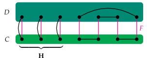
Figure 2: Condition in the local case. The blocks $C$, $D$ and a perfect matching $F$ between them are fixed.

We introduce some auxiliary random variables. Let $\mathbf{C}\coloneqq\mathbf{C_{1}}\cup\mathbf{C_{H}}$ and $\mathbf{D}\coloneqq\mathbf{D_{1}}\cup\mathbf{D_{H}}$. Note that $\mathbf{C},\mathbf{D}$ and $\mathbf{H}$ are uniformly distributed (independently of $\mathbf{M},\mathbf{U},\mathbf{\Pi},\mathbf{N}$), and together determine the $\mathbf{C_{1}},\mathbf{D_{1}},\mathbf{C_{H}},\mathbf{D_{H}}$. Furthermore, we introduce $\mathbf{F}$ as a uniformly random extension of $\mathbf{H}$ into a full matching between $\mathbf{C}$ and $\mathbf{D}$, depending only on $\mathbf{C}$, $\mathbf{D}$ and $\mathbf{H}$. This independence ensures that adding it as condition to the mutual information has no effect:

$$\begin{split}\mathbb{I}\left[\mathbf{M},\mathbf{U};\mathbf{\Pi}\,\middle|\,\mathbf{T},\mathbf{H},\mathbf{N},\mathscr{E}\right]&=\mathbb{I}\left[\mathbf{M},\mathbf{U};\mathbf{\Pi}\,\middle|\,\mathbf{T},\mathbf{H},\mathbf{F},\mathbf{N},\mathscr{E}\right]=\mathbb{I}\left[\mathbf{M},\mathbf{U};\mathbf{\Pi}\,\middle|\,\mathbf{C},\mathbf{D},\mathbf{F},\mathbf{H},\mathbf{N},\mathscr{E}\right]\\ &=\operatorname{\mathbb{E}}_{C\sim\mathbf{C},D\sim\mathbf{D},F\sim\mathbf{F}\mid\mathscr{E}}\left[\mathbb{I}\left[\mathbf{M},\mathbf{U};\mathbf{\Pi}\,\middle|\,\mathbf{C}=C,\mathbf{D}=D,\mathbf{F}=F,\mathbf{H},\mathbf{N},\mathscr{E}\right]\right].\end{split}$$

We show that the inner term is always at least $c_{k,\varepsilon}$. To this end, we fix $C,D,F$, and drop them from the condition to simplify notation. For convenience, we rewrite the events $\mathscr{E}_{0}$ and $\mathscr{E}$ in a simple form:

$$\mathscr{E}_{0} \coloneqq\mathbf{U}\in\{C,C(\mathbf{H})\}\land\mathbf{H}\subseteq\mathbf{M} \mathscr{E} \coloneqq\mathscr{E}_{0}\land\begin{cases}\mathbf{U}=C(\mathbf{H}),&\text{if }\mathbf{N}=0\\ \delta(C)\cap\mathbf{M}=\mathbf{H},&\text{if }\mathbf{N}=1.\end{cases}$$

Here and below for a $3$-matching $h\subseteq F$, let $C(h)$ denote the endpoints of the edges of $h$ lying in $C$. (I.e., $C(\mathbf{H})=\mathbf{C_{H}}$ but we shall use the notation for other $h$, too.) As $\mathbf{N}$ consists of only one coin, we simply identify it with $\mathbf{N}$.

To proceed, we will distinguish two types of pairs $(\pi,h)$: the good pairs are where the conditional distribution $(\mathbf{M},\mathbf{U})\mid\mathbf{\Pi}=\pi,H=h$ is close to the distribution $(\mathbf{M},\mathbf{U})\mid H=h$ with the condition on $\mathbf{\Pi}$ left out. Therefore the contribution of good pairs to mutual information is negligible. The bad pairs are where the two distributions differ significantly, and hence contribute much to mutual information. As we will see in Section 3.4, there are not too many good pairs, and this is the key to the proof.

We now state the exact definitions of goodness and badness, taking also the conditions in the mutual information into account, using a small positive number $\delta>0$ chosen later:

Definition 3.3.

A pair $(\pi,h)$ is $\mathbf{M}$-good if for all matchings $m\supseteq h$

$$1-\delta\leq\frac{\operatorname{\mathbb{P}}\left[\mathbf{M}=m\,\middle|\,\mathbf{\Pi}=\pi,\mathbf{H}=h,\mathbf{N}=0,\mathscr{E}\right]}{\operatorname{\mathbb{P}}\left[\mathbf{M}=m\,\middle|\,\mathbf{H}=h,\mathbf{N}=0,\mathscr{E}\right]}\leq 1+\delta.$$

Otherwise the pair is $\mathbf{M}$-bad, denoted as $\operatorname{\mathbf{M}-BAD}(\pi,h)$. Similarly, a pair $(\pi,h)$ is $\mathbf{U}$-good if for $u=C(h)$ and $u=C$

$$1-\delta\leq\frac{\operatorname{\mathbb{P}}\left[\mathbf{U}=u\,\middle|\,\mathbf{\Pi}=\pi,\mathbf{H}=h,\mathbf{N}=1,\mathscr{E}\right]}{\operatorname{\mathbb{P}}\left[\mathbf{U}=u\,\middle|\,\mathbf{H}=h,\mathbf{N}=1,\mathscr{E}\right]}\leq 1+\delta.$$

Otherwise the pair is $\mathbf{U}$-bad, denoted as $\operatorname{\mathbf{U}-BAD}(\pi,h)$.

The pair $(\pi,h)$ is good if it is both $\mathbf{M}$-good and $\mathbf{U}$-good. It is denoted by $\operatorname{GOOD}(\pi,h)$. The pair is bad, denoted as $\operatorname{BAD}(\pi,h)$ if it is not good.

Now we reduce the proposition to estimating the probability of bad pairs.

Proof of Proposition 3.2: the case $m=1$ and $l=0$.

We will use Pinsker’s inequality (Lemma 2.2) to lower bound the mutual information induced by those $(\pi,h)$ which are $\mathbf{M}$-bad or $\mathbf{U}$-bad (depending on the outcome of the coin $\mathbf{N}$). Therefore we rewrite the mutual information using relative entropy:

$$\mathbb{I}\left[\mathbf{M},\mathbf{U};\mathbf{\Pi}\,\middle|\,\mathbf{H},\mathbf{N},\mathscr{E}\right]=\operatorname{\mathbb{E}}_{\mathbf{\Pi},\mathbf{H},\mathbf{N}\mid\mathscr{E}}\left[\operatorname{\mathbb{D}}\left(\mathbf{M},\mathbf{U}\mid\mathbf{\Pi},\mathbf{H},\mathbf{N},\mathscr{E}\,\middle\|\,\mathbf{M},\mathbf{U}\mid\mathbf{H},\mathbf{N},\mathscr{E}\right)\right]\\ =\sum_{i\in\{0,1\}}\operatorname{\mathbb{P}}\left[\mathbf{N}=i\,\middle|\,\mathscr{E}\right]\cdot\operatorname{\mathbb{E}}_{\mathbf{\Pi},\mathbf{H}\mid\mathbf{N}=i,\mathscr{E}}\left[\operatorname{\mathbb{D}}\left(\mathbf{M},\mathbf{U}\mid\mathbf{\Pi},\mathbf{H},\mathbf{N}=i,\mathscr{E}\,\middle\|\,\mathbf{M},\mathbf{U}\mid\mathbf{H},\mathbf{N}=i,\mathscr{E}\right)\right].$$

By definition of badness, for $\mathbf{M}$-bad pairs there is an $m$ where the probabilities differ by at least

$$\delta\operatorname{\mathbb{P}}\left[\mathbf{M}=m\,\middle|\,\mathbf{H}=h,\mathbf{N}=0,\mathscr{E}\right]=\delta\alpha,$$

where $\alpha=1/(2k-7)!!$, the reciprocal of the number of perfect matchings on $2k-6$ nodes. Similarly, for $\mathbf{U}$-bad pairs, the probabilities differ by at least

$$\delta\operatorname{\mathbb{P}}\left[\mathbf{U}=u\,\middle|\,\mathbf{H}=h,\mathbf{N}=1,\mathscr{E}\right]=\delta\frac{1}{2}.$$

Thus via Lemma 2.2 we have

$$\operatorname{\mathbb{E}}_{\mathbf{\Pi},\mathbf{H}\mid\mathbf{N}=0,\mathscr{E}}\left[\operatorname{\mathbb{D}}\left(\mathbf{M},\mathbf{U}\mid\mathbf{\Pi},\mathbf{H},\mathbf{N}=0,\mathscr{E}\,\middle\|\,\mathbf{M},\mathbf{U}\mid\mathbf{H},\mathbf{N}=0,\mathscr{E}\right)\right]\\ \geq\operatorname{\mathbb{P}}\left[\operatorname{\mathbf{M}-BAD}(\mathbf{\Pi},\mathbf{H})\,\middle|\,\mathbf{N}=0,\mathscr{E}\right]2(\log e)(\delta\alpha)^{2},$$

and

$$\operatorname{\mathbb{E}}_{\mathbf{\Pi},\mathbf{H}\mid\mathbf{N}=1,\mathscr{E}}\left[\operatorname{\mathbb{D}}\left(\mathbf{M},\mathbf{U}\mid\mathbf{\Pi},\mathbf{H},\mathbf{N}=1,\mathscr{E}\,\middle\|\,\mathbf{M},\mathbf{U}\mid\mathbf{H},\mathbf{N}=1,\mathscr{E}\right)\right]\\ \geq\operatorname{\mathbb{P}}\left[\operatorname{\mathbf{U}-BAD}(\mathbf{\Pi},\mathbf{H})\,\middle|\,\mathbf{N}=1,\mathscr{E}\right]2(\log e)\left(\frac{\delta}{2}\right)^{2}.$$

The main part of the proof is to lower bound the probability of being bad. To simplify computations, we rewrite the probabilities appearing above in a more manageable form:

$$\operatorname{\mathbb{P}}\left[\operatorname{\mathbf{M}-BAD}(\mathbf{\Pi},\mathbf{H})\,\middle|\,\mathbf{N}=0,\mathscr{E}\right] =\operatorname{\mathbb{P}}\left[\operatorname{\mathbf{M}-BAD}(\mathbf{\Pi},\mathbf{H})\,\middle|\,\mathbf{U}=C(\mathbf{H}),\mathscr{E}_{0}\right]$$

$$=\frac{\operatorname{\mathbb{P}}\left[\operatorname{\mathbf{M}-BAD}(\mathbf{\Pi},\mathbf{H}),\mathbf{U}=C(\mathbf{H})\,\middle|\,\mathscr{E}_{0}\right]}{\operatorname{\mathbb{P}}\left[\mathbf{U}=C(\mathbf{H})\,\middle|\,\mathscr{E}_{0}\right]}$$

$$\operatorname{\mathbb{P}}\left[\operatorname{\mathbf{U}-BAD}(\mathbf{\Pi},\mathbf{H})\,\middle|\,\mathbf{N}=1,\mathscr{E}\right] =\frac{\operatorname{\mathbb{P}}\left[\operatorname{\mathbf{U}-BAD}(\mathbf{\Pi},\mathbf{H}),\mathbf{H}=\delta(C)\cap\mathbf{M}\,\middle|\,\mathscr{E}_{0}\right]}{\operatorname{\mathbb{P}}\left[\mathbf{H}=\delta(C)\cap\mathbf{M}\,\middle|\,\mathscr{E}_{0}\right]}.$$

We shall obtain a constant $B_{k,\varepsilon}>0$ lower bounding the sum of the probabilities of being $\mathbf{M}$-bad or $\mathbf{U}$-bad

$$\operatorname{\mathbb{P}}\left[\operatorname{\mathbf{M}-BAD}(\mathbf{\Pi},\mathbf{H}),\mathbf{U}=C(\mathbf{H})\,\middle|\,\mathscr{E}_{0}\right]+\operatorname{\mathbb{P}}\left[\operatorname{\mathbf{U}-BAD}(\mathbf{\Pi},\mathbf{H}),\mathbf{H}=\delta(C)\cap\mathbf{M}\,\middle|\,\mathscr{E}_{0}\right]\geq B_{k,\varepsilon}.$$

Note that the probabilities cannot be bounded separately as individually they can be $0$. Once obtained this bound then leads to

$$\begin{split}\mathbb{I}\left[\mathbf{M},\mathbf{U};\mathbf{\Pi}\,\middle|\,\mathbf{H},\mathbf{N},\mathscr{E}\right]&\geq\operatorname{\mathbb{P}}\left[\mathbf{N}=0\,\middle|\,\mathscr{E}\right]\cdot\operatorname{\mathbb{P}}\left[\operatorname{\mathbf{M}-BAD}(\mathbf{\Pi},\mathbf{H})\,\middle|\,\mathbf{N}=0,\mathscr{E}\right]2(\log e)(\delta\alpha)^{2}\\ &+\operatorname{\mathbb{P}}\left[\mathbf{N}=1\,\middle|\,\mathscr{E}\right]\cdot\operatorname{\mathbb{P}}\left[\operatorname{\mathbf{U}-BAD}(\mathbf{\Pi},\mathbf{H})\,\middle|\,\mathbf{N}=1,\mathscr{E}\right]2(\log e)\left(\frac{\delta}{2}\right)^{2}\\ &\geq B_{k,\varepsilon}(2\log e)\delta^{2}\min\left\{\frac{\operatorname{\mathbb{P}}\left[\mathbf{N}=0\,\middle|\,\mathscr{E}\right]\alpha^{2}}{\operatorname{\mathbb{P}}\left[\mathbf{U}=C(\mathbf{H})\,\middle|\,\mathscr{E}_{0}\right]},\frac{\operatorname{\mathbb{P}}\left[\mathbf{N}=1\,\middle|\,\mathscr{E}\right]/4}{\operatorname{\mathbb{P}}\left[\delta(C)\cap\mathbf{M}=\mathbf{H}\,\middle|\,\mathscr{E}_{0}\right]}\right\}\eqqcolon c_{k,\varepsilon}.\end{split}$$

This is a positive constant depending only on $k$ and $\varepsilon$ provided $B_{k,\varepsilon}>0$, which we prove in the next section.

3.4 Bounding probability of being good

To obtain the claimed lower bound $B_{k,\varepsilon}>0$ on the probability of being bad, we investigate how much the good pairs contribute to the distribution of $\mathbf{M},\mathbf{U}$. We start by rewriting goodness into a form with less conditions on probabilities. For any $3$-matching $h$ between $C$ and $D$, any perfect matching $m\supseteq h$ we have

$$\operatorname{\mathbb{P}}\left[\mathbf{M}=m\,\middle|\,\mathbf{\Pi}=\pi,\mathbf{H}=h,\mathbf{N}=0,\mathscr{E}\right] =\operatorname{\mathbb{P}}\left[\mathbf{M}=m\,\middle|\,\mathbf{\Pi}=\pi,\mathbf{H}=h,\mathbf{N}=0,\mathbf{U}=C(h),h\subseteq\mathbf{M}\right]$$

$$=\operatorname{\mathbb{P}}\left[\mathbf{M}=m\,\middle|\,\mathbf{\Pi}=\pi,\mathbf{U}=C(h),h\subseteq\mathbf{M}\right]$$

$$=\operatorname{\mathbb{P}}\left[\mathbf{M}=m\,\middle|\,\mathbf{\Pi}=\pi,h\subseteq\mathbf{M}\right]=\frac{\operatorname{\mathbb{P}}\left[\mathbf{M}=m\,\middle|\,\mathbf{\Pi}=\pi\right]}{\operatorname{\mathbb{P}}\left[h\subseteq\mathbf{M}\,\middle|\,\mathbf{\Pi}=\pi\right]},$$

by first expanding $\mathscr{E}$, then removing $\mathbf{H},\mathbf{N}$ using their independence of $\mathbf{M},\mathbf{\Pi},\mathbf{U}$, and finally removing $\mathbf{U}$, as it is independent of $\mathbf{M}$ given $\mathbf{\Pi}$. Similarly, for $u\in\{C(h),C\}$

$$\operatorname{\mathbb{P}}\left[\mathbf{U}=u\,\middle|\,\mathbf{\Pi}=\pi,\mathbf{H}=h,\mathbf{N}=1,\mathscr{E}\right]=\frac{\operatorname{\mathbb{P}}\left[\mathbf{U}=u\,\middle|\,\mathbf{\Pi}=\pi\right]}{\operatorname{\mathbb{P}}\left[\mathbf{U}\in\{C(h),C\}\,\middle|\,\mathbf{\Pi}=\pi\right]}.$$

This is mostly useful for comparing probabilities for the various values of $m,u$. Let $\beta\coloneqq\left(\frac{1-\delta}{1+\delta}\right)^{2}$. When $(\pi,h)$ is good, we obtain

$$\sqrt{\beta}\operatorname{\mathbb{P}}\left[\mathbf{U}=C\,\middle|\,\mathbf{\Pi}=\pi\right]\leq\operatorname{\mathbb{P}}\left[\mathbf{U}=C(h)\,\middle|\,\mathbf{\Pi}=\pi\right] \leq\frac{1}{\sqrt{\beta}}\operatorname{\mathbb{P}}\left[\mathbf{U}=C\,\middle|\,\mathbf{\Pi}=\pi\right],$$ and

$$\sqrt{\beta}\operatorname{\mathbb{P}}\left[\mathbf{M}=F\,\middle|\,\mathbf{\Pi}=\pi\right]\leq\operatorname{\mathbb{P}}\left[\mathbf{M}=m\,\middle|\,\mathbf{\Pi}=\pi\right] \leq\frac{1}{\sqrt{\beta}}\operatorname{\mathbb{P}}\left[\mathbf{M}=F\,\middle|\,\mathbf{\Pi}=\pi\right], \text{for }h \subseteq m.$$

Let us fix $\pi$, and let $h_{1},\dotsc,h_{N}$ be all the $3$-submatchings of $F$ with $(\pi,h_{i})$ good. Let $u_{i}=C(h_{i})$ denote the vertices of $h_{i}$ in $C$. We divide the $h_{i}$ into two classes: the first class consists of the $h_{i}$ having two common edges with every other $h_{j}$, i.e., the intersection $u_{i}\cap u_{j}$ has $2$ elements for all $j\neq i$. Without loss of generality, the first class is $h_{1},\dotsc,h_{\ell}$. The second class consists of the $h_{i}$ which do not have two common edges with all the other $h_{j}$.

The Erdős–Ko–Rado Theorem (Erdős et al., 1961, Theorem 2) bounds the size of the first class by $\ell\leq k-2$ for $k\geq 6$, (slightly improving over the $3k$ in the combinatorial part of (Rothvoß, 2014, Lemma 8)). We consider matchings $m$ satisfying $h_{i}=\delta(C)\cap m$ for an $i$. For $i\leq\ell$, i.e., $h_{i}$ is in the first class, we estimate

$$\begin{split}\operatorname{\mathbb{P}}\left[\mathbf{M}=F,\mathbf{U}=C\,\middle|\,\mathbf{\Pi}=\pi\right]&=\operatorname{\mathbb{P}}\left[\mathbf{M}=F\,\middle|\,\mathbf{\Pi}=\pi\right]\operatorname{\mathbb{P}}\left[\mathbf{U}=C\,\middle|\,\mathbf{\Pi}=\pi\right]\\ &\geq\sqrt{\beta}\operatorname{\mathbb{P}}\left[\mathbf{M}=m\,\middle|\,\mathbf{\Pi}=\pi\right]\cdot\sqrt{\beta}\operatorname{\mathbb{P}}\left[\mathbf{U}=u_{i}\,\middle|\,\mathbf{\Pi}=\pi\right]\\ &=\beta\operatorname{\mathbb{P}}\left[\mathbf{M}=m,\mathbf{U}=u_{i}\,\middle|\,\mathbf{\Pi}=\pi\right].\end{split}$$

Taking the average over all $m$, we obtain

$$\operatorname{\mathbb{P}}\left[\mathbf{M}=F,\mathbf{U}=C\,\middle|\,\mathbf{\Pi}=\pi\right]\geq\frac{\beta}{A}\operatorname{\mathbb{P}}\left[h_{i}=\delta(C)\cap\mathbf{M},\mathbf{U}=u_{i}\,\middle|\,\mathbf{\Pi}=\pi\right],\qquad i\leq\ell,$$ (3)

with $A\coloneqq(k-4)!!^{2}$ being the number of matchings $m$ with $\delta(C)\cap m=h_{i}$.

For $i>\ell$ there is a $j$ such that $\left|u_{i}\cap u_{j}\right|\leq 1$. Thus there is an edge $e\in E[u_{i}]$ not incident with any vertices of $u_{j}$. We replace the two edges $e_{1},e_{2}$ in $F$ at the endpoints of $e$ by the two edges $e$ and $f$ connecting their endpoints in $C$ and $D$, respectively, see Figure 3.

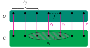
Figure 3: Constructing the matching $m^{\prime}$ by replacing $e_{1}$, $e_{2}$ in $F$ by the dashed edges: $e$ in $u_{i}$ and its counter part $f$ in $D$.

Let $m^{\prime}\coloneqq F\setminus\{e_{1},e_{2}\}\cup\{e,f\}$ be the new matching, it contains $e$. Note that $\left|\delta(u_{i})\cap m^{\prime}\right|=1$ and

$$\begin{split}\operatorname{\mathbb{P}}\left[\mathbf{M}=m^{\prime},\mathbf{U}=u_{i}\,\middle|\,\mathbf{\Pi}=\pi\right]&=\operatorname{\mathbb{P}}\left[\mathbf{M}=m^{\prime}\,\middle|\,\mathbf{\Pi}=\pi\right]\operatorname{\mathbb{P}}\left[\mathbf{U}=u_{i}\,\middle|\,\mathbf{\Pi}=\pi\right]\\ &\geq\sqrt{\beta}\operatorname{\mathbb{P}}\left[\mathbf{M}=F\,\middle|\,\mathbf{\Pi}=\pi\right]\operatorname{\mathbb{P}}\left[\mathbf{U}=u_{i}\,\middle|\,\mathbf{\Pi}=\pi\right]\\ &\geq\beta\operatorname{\mathbb{P}}\left[\mathbf{M}=m\,\middle|\,\mathbf{\Pi}=\pi\right]\operatorname{\mathbb{P}}\left[\mathbf{U}=u_{i}\,\middle|\,\mathbf{\Pi}=\pi\right]\\ &=\beta\operatorname{\mathbb{P}}\left[\mathbf{M}=m,\mathbf{U}=u_{i}\,\middle|\,\mathbf{\Pi}=\pi\right].\end{split}$$

Taking the average over all $m$ provides

$$\begin{split}\operatorname{\mathbb{P}}\left[\left|\delta(\mathbf{U})\cap\mathbf{M}\right|=1,\left|\mathbf{M}\setminus F\right|=2,\mathbf{U}=u_{i}\,\middle|\,\mathbf{\Pi}=\pi\right]&\geq\operatorname{\mathbb{P}}\left[\mathbf{M}=m^{\prime},\mathbf{U}=u_{i}\,\middle|\,\mathbf{\Pi}=\pi\right]\\ &\geq\frac{\beta}{A}\operatorname{\mathbb{P}}\left[h_{i}=\delta(C)\cap\mathbf{M},\mathbf{U}=u_{i}\,\middle|\,\mathbf{\Pi}=\pi\right].\end{split}$$ (4)

Now we add $\mathbf{H}$ to (3) and (4), using its independence of the variables involved there, we have

$$\frac{\beta}{A}\operatorname{\mathbb{P}}\left[\mathbf{H}=\delta(C)\cap\mathbf{M},\mathbf{U}=C(\mathbf{H}),\mathbf{H}=h_{i}\,\middle|\,\mathbf{\Pi}=\pi\right]\\ \leq\begin{cases}\operatorname{\mathbb{P}}\left[\mathbf{M}=F,\mathbf{U}=C\,\middle|\,\mathbf{\Pi}=\pi\right]/\binom{k}{3},&\text{for }i\leq\ell,\\ \operatorname{\mathbb{P}}\left[\left|\delta(\mathbf{U})\cap\mathbf{M}\right|=1,\left|\mathbf{M}\setminus F\right|=2,\mathbf{H}=h_{i},\mathbf{U}=C(\mathbf{H})\,\middle|\,\mathbf{\Pi}=\pi\right],&\text{for }i>\ell.\end{cases}$$ (5)

We sum up over all $i$ to obtain

$$\frac{\beta}{A}\operatorname{\mathbb{P}}\left[\mathbf{H}=\delta(C)\cap\mathbf{M},\mathbf{U}=C(\mathbf{H}),\operatorname{GOOD}(\mathbf{\Pi},\mathbf{H})\,\middle|\,\mathbf{\Pi}=\pi\right]\\ \leq\frac{\ell}{\binom{k}{3}}\operatorname{\mathbb{P}}\left[\mathbf{M}=F,\mathbf{U}=C\,\middle|\,\mathbf{\Pi}=\pi\right]+\operatorname{\mathbb{P}}\left[\left|\delta(\mathbf{U})\cap\mathbf{M}\right|=1,\left|\mathbf{M}\setminus F\right|=2,\mathbf{U}=C(\mathbf{H})\,\middle|\,\mathbf{\Pi}=\pi\right].$$ (6)

We take expectation over $\pi\sim\mathbf{\Pi}$. Recall that $\ell\leq k-2$, hence

$$\begin{split}\frac{\beta}{A}&\left(\operatorname{\mathbb{P}}\left[\mathbf{H}=\delta(C)\cap\mathbf{M},\mathbf{U}=C(\mathbf{H})\right]-\operatorname{\mathbb{P}}\left[\mathbf{H}=\delta(C)\cap\mathbf{M},\mathbf{U}=C(\mathbf{H}),\operatorname{BAD}(\mathbf{\Pi},\mathbf{H})\right]\right)\\ &=\frac{\beta}{A}\operatorname{\mathbb{P}}\left[\mathbf{H}=\delta(C)\cap\mathbf{M},\mathbf{U}=C(\mathbf{H}),\operatorname{GOOD}(\mathbf{\Pi},\mathbf{H})\right]\\ &\leq\frac{k-2}{\binom{k}{3}}\operatorname{\mathbb{P}}\left[\mathbf{M}=F,\mathbf{U}=C\right]+\operatorname{\mathbb{P}}\left[\left|\delta(\mathbf{U})\cap\mathbf{M}\right|=1,\left|\mathbf{M}\setminus F\right|=2,\mathbf{U}=C(\mathbf{H})\right].\end{split}$$ (7)

We compute the values of the various probabilities from $S^{+\varepsilon}$. The probability of a fixed pair $(M,U)$ is proportional to their slack value, i.e.,

$$\operatorname{\mathbb{P}}\left[\mathbf{M}=M,\mathbf{U}=U\right]=(\left|\delta(U)\cap M\right|-1+\varepsilon)\gamma,$$

for some positive constant $\gamma$ depending only on $k$ and $\varepsilon$. In particular,

$$\operatorname{\mathbb{P}}\left[\mathbf{M}=F,\mathbf{U}=C\right]=(k-1+\varepsilon)\gamma.$$

(We do not need the exact value of $\gamma$, but actually $\gamma=\left[\sum_{M,U}(\left|\delta(\mathbf{U})\cap\mathbf{M}\right|-1+\varepsilon)\right]^{-1}=[(k/2-1+\varepsilon)\cdot(2k-1)!!\cdot 2^{2k-1}]^{-1}$, using that there are $(2k-1)!!2^{2k-1}$ pairs $(M,U)$ altogether, and $\binom{2k}{2}$ edges of $K_{2k}$. Each edge belongs to $\delta(U)\cap M$ for exactly an $1/[2(2k-1)]$ part of the pairs $(M,U)$.)

For the other events, it is easier to compute the probability conditioned on $\mathbf{H}$:

$$\operatorname{\mathbb{P}}\left[\mathbf{H}=\delta(C)\cap\mathbf{M},\mathbf{U}=C(\mathbf{H})\right]=\operatorname{\mathbb{E}}_{\mathbf{H}}\left[\operatorname{\mathbb{P}}\left[\mathbf{H}=\delta(C)\cap\mathbf{M},\mathbf{U}=C(\mathbf{H})\,\middle|\,\mathbf{H}\right]\right]=(2+\varepsilon)\gamma A.$$

Recall that $A$ is the number of pairs satisfying the event for $\mathbf{H}$ fixed. Here we have used that $(\mathbf{M},\mathbf{U})$ is independent of $\mathbf{H}$.

The probability of the third event is determined similarly. Note that for any fixed $3$-element $\mathbf{U}$, there are $3$ matchings $m$ with $\left|\delta(\mathbf{U})\cap m\right|=1$ and $\left|m\setminus F\right|=2$, actually arising by an analogous construction depicted in Figure 3.

$$\operatorname{\mathbb{P}}\left[\left|\delta(\mathbf{U})\cap\mathbf{M}\right|=1,\left|\mathbf{M}\setminus F\right|=2,\mathbf{U}=C(\mathbf{H})\right]=\varepsilon\gamma\cdot 3.$$

Substituting the probabilities back into our formula, we obtain

$$\operatorname{\mathbb{P}}\left[\mathbf{H}=\delta(C)\cap\mathbf{M},\mathbf{U}=C(\mathbf{H}),\operatorname{BAD}(\mathbf{\Pi},\mathbf{H})\right]\geq(2+\varepsilon)\gamma A-\left(\frac{6(k-1+\varepsilon)}{k(k-1)}\gamma+\varepsilon\gamma\cdot 3\right)\frac{A}{\beta}.$$

Finally, we add back the event $\mathscr{E}_{0}$ as a condition. Recall that $\varepsilon\leq 1-4/k$, hence

$$\operatorname{\mathbb{P}}\left[\mathbf{H}=\delta(C)\cap\mathbf{M},\mathbf{U}=C(\mathbf{H}),\operatorname{BAD}(\mathbf{\Pi},\mathbf{H})\,\middle|\,\mathscr{E}_{0}\right]\\ \geq\left(2+\varepsilon-\left(\frac{6(k-1+\varepsilon)}{k(k-1)}+\varepsilon\cdot 3\right)\frac{1}{\beta}\right)\frac{\gamma A}{\operatorname{\mathbb{P}}\left[\mathscr{E}_{0}\right]}\\ =\left(2-\left(\frac{6(k-1+\varepsilon)}{k(k-1)}+(3-\beta)\varepsilon\right)\frac{1}{\beta}\right)\frac{\gamma A}{\operatorname{\mathbb{P}}\left[\mathscr{E}_{0}\right]}\\ \geq\left(2-\left(\frac{6(k-1+(1-4/k))}{k(k-1)}+(3-\beta)(1-4/k)\right)\frac{1}{\beta}\right)\frac{\gamma A}{\operatorname{\mathbb{P}}\left[\mathscr{E}_{0}\right]}\\ =\left(2-(3k-4)(1-\beta)-\frac{6(k-4)}{k(k-1)}\right)\frac{\gamma A}{k\beta\operatorname{\mathbb{P}}\left[\mathscr{E}_{0}\right]}.$$

The last expression has a positive lower bound $B_{k,\varepsilon}$ depending only on $k$ and $\varepsilon$. (Note that $\operatorname{\mathbb{P}}\left[\mathscr{E}_{0}\right]/\gamma$ involves $\varepsilon$.) To this end, we choose $\delta$ sufficiently close to $0$, ensuring that $\beta$ is sufficiently close to $1$, making the last parenthesized expression positive. The number $A$ depends just on $k$.

All in all, $\operatorname{\mathbb{P}}\left[\mathbf{H}=\delta(C)\cap\mathbf{M},\mathbf{U}=C(\mathbf{H}),\operatorname{BAD}(\mathbf{\Pi},\mathbf{H})\,\middle|\,\mathscr{E}_{0}\right]\geq B_{k,\varepsilon}>0$. Finally,

$$\operatorname{\mathbb{P}}\left[\mathbf{U}=C(\mathbf{H}),\operatorname{\mathbf{M}-BAD}(\mathbf{\Pi},\mathbf{H})\,\middle|\,\mathscr{E}_{0}\right]+\operatorname{\mathbb{P}}\left[\mathbf{H}=\delta(C)\cap\mathbf{M},\operatorname{\mathbf{U}-BAD}(\mathbf{\Pi},\mathbf{H})\,\middle|\,\mathscr{E}_{0}\right]\\ \geq\operatorname{\mathbb{P}}\left[\mathbf{H}=\delta(C)\cap\mathbf{M},\mathbf{U}=C(\mathbf{H}),\operatorname{BAD}(\mathbf{\Pi},\mathbf{H})\,\middle|\,\mathscr{E}_{0}\right]\geq B_{k,\varepsilon}.$$

∎

4 Concluding remarks

We believe that the information-theoretic framework is general enough to also be able to reproduce the results in Chan et al. (2013) and potentially improving on the strength of the lower bound. Also, recently in Lee et al. (2014) it has been shown that the results in Chan et al. (2013) also extend to the case of semidefinite programming formulation. However, it is open whether the semidefinite formulation complexity of the matching problem is exponential and a careful modification of the presented approach might shed some light on this question.

References

- Avis and Tiwary [2013] D. Avis and H. R. Tiwary. On the extension complexity of combinatorial polytopes. ArXiv e-prints, Feb. 2013.
- Bar-Yossef et al. [2004] Z. Bar-Yossef, T. Jayram, R. Kumar, and D. Sivakumar. An information statistics approach to data stream and communication complexity. Journal of Computer and System Sciences, 68(4):702–732, 2004. doi: 10.1016/j.jcss.2003.11.006. URL http://www.sciencedirect.com/science/article/pii/S0022000003001855.
- Bienstock [2008] D. Bienstock. Approximate formulations for 0-1 knapsack sets. Operations Research Letters, 36(3):317–320, 2008.
- Braun and Pokutta [2013] G. Braun and S. Pokutta. Common information and unique disjointness. Proceedings of FOCS, pages 688–697, 2013.
- Braun et al. [2012] G. Braun, S. Fiorini, S. Pokutta, and D. Steurer. Approximation limits of linear programs (beyond hierarchies). In 53rd IEEE Symp. on Foundations of Computer Science (FOCS 2012), pages 480–489, 2012. ISBN 978-1-4673-4383-1. doi: 10.1109/FOCS.2012.10.
- Braun et al. [2013] G. Braun, R. Jain, T. Lee, and S. Pokutta. Information-theoretic approximations of the nonnegative rank. submitted / preprint available at ECCC http://eccc.hpi-web.de/report/2013/158., 2013.
- Braun et al. [2014a] G. Braun, S. Fiorini, and S. Pokutta. Average case polyhedral complexity of the maximum stable set problem. Proceedings of RANDOM / arXiv:1311.4001, 2014a.
- Braun et al. [2014b] G. Braun, S. Pokutta, and D. Zink. LP and SDP inapproximability of combinatorial problems. arXiv preprint arXiv:1410.8816, 2014b. accepted for STOC 2015.
- Braverman and Moitra [2012] M. Braverman and A. Moitra. An information complexity approach to extended formulations. Electronic Colloquium on Computational Complexity (ECCC), 19(131), 2012.
- Braverman et al. [2012] M. Braverman, A. Garg, D. Pankratov, and O. Weinstein. From information to exact communication. In Electronic Colloquium on Computational Complexity (ECCC), volume 19, page 171, 2012.
- Briët et al. [2013] J. Briët, D. Dadush, and S. Pokutta. On the existence of 0/1 polytopes with high semidefinite extension complexity. Proceedings of ESA / arxiv:1305.3268, 2013.
- Chan et al. [2013] S. O. Chan, J. R. Lee, P. Raghavendra, and D. Steurer. Approximate constraint satisfaction requires large LP relaxations. In IEEE 54th Annual Symp. on Foundations of Computer Science (FOCS 2013), pages 350–359. IEEE, 2013. doi: 10.1109/FOCS.2013.45.
- Conforti et al. [2010] M. Conforti, G. Cornuéjols, and G. Zambelli. Extended formulations in combinatorial optimization. 4OR, 8:1–48, 2010. doi: 10.1007/s10288-010-0122-z.
- Cover and Thomas [2006] T. Cover and J. Thomas. Elements of information theory. Wiley-interscience, 2006.
- Edmonds [1965] J. Edmonds. Maximum matching and a polyhedron with 0, 1 vertices. Journal of Research National Bureau of Standards, 69B:125–130, 1965.
- Erdős et al. [1961] P. Erdős, C. Ko, and R. Rado. Intersection theorems for systems of finite sets. Q. J. Math., Oxf. II. Ser., 12:313–320, 1961. ISSN 0033-5606; 1464-3847/e. doi: 10.1093/qmath/12.1.313.
- Faenza et al. [2012] Y. Faenza, S. Fiorini, R. Grappe, and H. R. Tiwary. Extended formulations, nonnegative factorizations, and randomized communication protocols. In A. Mahjoub, V. Markakis, I. Milis, and V. Paschos, editors, Combinatorial Optimization, volume 7422 of Lecture Notes in Computer Science, pages 129–140. Springer Berlin Heidelberg, 2012. ISBN 978-3-642-32146-7. doi: 10.1007/978-3-642-32147-4_13. URL http://dx.doi.org/10.1007/978-3-642-32147-4_13.
- Fiorini et al. [2012a] S. Fiorini, V. Kaibel, K. Pashkovich, and D. O. Theis. Combinatorial bounds on nonnegative rank and extended formulations, 2012a. arXiv:1111.0444v2.
- Fiorini et al. [2012b] S. Fiorini, S. Massar, S. Pokutta, H. R. Tiwary, and R. de Wolf. Linear vs. semidefinite extended formulations: Exponential separation and strong lower bounds. Proceedings of STOC 2012, 2012b.
- Fiorini et al. [2012c] S. Fiorini, T. Rothvoß, and H. R. Tiwary. Extended formulations for polygons. Discrete & Computational Geometry, 48(3):658–668, 2012c. ISSN 0179-5376. doi: 10.1007/s00454-012-9421-9. URL http://dx.doi.org/10.1007/s00454-012-9421-9.
- Håstad [1999] J. Håstad. Clique is hard to approximate within . Acta Mathematica, 182(1):105–142, 1999.
- Jain et al. [2013] R. Jain, Y. Shi, Z. Wei, and S. Zhang. Efficient protocols for generating bipartite classical distributions and quantum states. Proceedings of SODA 2013, 2013.
- Kaibel [2011] V. Kaibel. Extended formulations in combinatorial optimization. Optima, 85:2–7, 2011.
- Kaibel and Weltge [2013] V. Kaibel and S. Weltge. A short proof that the extension complexity of the correlation polytope grows exponentially. arXiv preprint arXiv:1307.3543, 2013.
- Kaibel et al. [2010] V. Kaibel, K. Pashkovich, and D. Theis. Symmetry matters for the sizes of extended formulations. In Proc. IPCO 2010, pages 135–148, 2010.
- Karchmer et al. [1995] M. Karchmer, E. Kushilevitz, and N. Nisan. Fractional covers and communication complexity. SIAM J. Discrete Math., 8:76–92, 1995. doi: 10.1137/S0895480192238482.
- Kolliopoulos and Moysoglou [2013] S. G. Kolliopoulos and Y. Moysoglou. Exponential lower bounds on the size of approximate formulations in the natural encoding for capacitated facility location. CoRR, abs/1312.1819, 2013.
- Lee et al. [2014] J. Lee, P. Raghavendra, and D. Steurer. Lower bounds on the size of semidefinite programming relaxations. STOC 2015, arXiv:1411.6317, 2014.
- Pashkovich [2012] K. Pashkovich. Extended Formulations for Combinatorial Polytopes. PhD thesis, Magdeburg Universität, 2012.
- Pokutta and Van Vyve [2013] S. Pokutta and M. Van Vyve. A note on the extension complexity of the knapsack polytope. to appear in Operations Research Letters, 2013.
- Razborov [1992] A. A. Razborov. On the distributional complexity of disjointness. Theoret. Comput. Sci., 106(2):385–390, 1992.
- Rothvoß [2012] T. Rothvoß. Some 0/1 polytopes need exponential size extended formulations. Math. Programming, 142(1–2):255–268, 2012. arXiv:1105.0036.
- Rothvoß [2014] T. Rothvoß. The matching polytope has exponential extension complexity. Proceedings of STOC, pages 263–272, 2014.
- Wyner [1975] A. Wyner. The common information of two dependent random variables. Information Theory, IEEE Transactions on, 21(2):163–179, 1975.
- Yannakakis [1988] M. Yannakakis. Expressing combinatorial optimization problems by linear programs (extended abstract). In Proc. STOC 1988, pages 223–228, 1988.
- Yannakakis [1991] M. Yannakakis. Expressing combinatorial optimization problems by linear programs. J. Comput. System Sci., 43(3):441–466, 1991. doi: 10.1016/0022-0000(91)90024-Y.