Multiple transitions of the susceptible-infected-susceptible epidemic model on complex networks

Abstract

The epidemic threshold of the susceptible-infected-susceptible (SIS) dynamics on random networks having a power law degree distribution with exponent $\gamma>3$ has been investigated using different mean-field approaches, which predict different outcomes. We performed extensive simulations in the quasistationary state for a comparison with these mean-field theories. We observed concomitant multiple transitions in individual networks presenting large gaps in the degree distribution and the obtained multiple epidemic thresholds are well described by different mean-field theories. We observed that the transitions involving thresholds which vanishes at the thermodynamic limit involve localized states, in which a vanishing fraction of the network effectively contribute to epidemic activity, whereas an endemic state, with a finite density of infected vertices, occurs at a finite threshold. The multiple transitions are related to the activations of distinct sub-domains of the network, which are not directly connected.

I Introduction

Phase transitions involving equilibrium and non-equilibrium processes on complex networks have begun drawing an increasing interest soon after the boom of network science at late 90’s Dorogovtsev et al. (2008). Percolation Albert et al. (2000), epidemic spreading Pastor-Satorras and Vespignani (2001a, b), and spin systems Dorogovtsev et al. (2002) are only a few examples of breakthrough in the investigation of critical phenomena in complex networks. Absorbing state phase transitions Henkel et al. (2008) have become a paradigmatic issue in the interplay between nonequilibrium systems and complex networks Castellano and Pastor-Satorras (2008); Hong et al. (2007); Juhász et al. (2012); Mata et al. (2014); Ferreira et al. (2011), being the epidemic spreading a prominent example where high complexity emerges from very simple dynamical rules on heterogeneous substrates Pastor-Satorras and Vespignani (2001a, b); Castellano and Pastor-Satorras (2010); Goltsev et al. (2012); Ferreira et al. (2012); Boguñá et al. (2013); Lee et al. (2013a).

The existence or absence of finite epidemic thresholds involving an endemic phase of the susceptible-infected-susceptible (SIS) model on scale-free (SF) networks with a degree distribution $P(k)\sim k^{-\gamma}$, where $\gamma$ is the degree exponent, has been target of a recent and intense investigation Castellano and Pastor-Satorras (2010); Cator and Van Mieghem (2012); Mieghem (2012); Goltsev et al. (2012); Ferreira et al. (2012); Boguñá et al. (2013); Lee et al. (2013a). In the SIS epidemic model, individuals can only be in one of two states: infected or susceptible. Infected individuals become spontaneously healthy at rate $1$ (this choice fixes the time scale), while the susceptible ones are infected at rate $\lambda n_{i}$, where $n_{i}$ is the number of infected contacts of a vertex $i$.

Distinct theoretical approaches for the SIS model were devised to determine an epidemic threshold $\lambda_{c}$ separating an absorbing, disease-free state from an active phase Castellano and Pastor-Satorras (2010); Cator and Van Mieghem (2012); Mieghem (2012); Goltsev et al. (2012); Ferreira et al. (2012); Boguñá et al. (2013); Lee et al. (2013a); Chakrabarti et al. (2008); Mata and Ferreira (2013). The quenched mean-field (QMF) theory Chakrabarti et al. (2008) explicitly includes the entire structure of the network through its adjacency matrix while the heterogeneous mean-field (HMF) theory Pastor-Satorras and Vespignani (2001a, b) performs a coarse-graining of the network grouping vertices accordingly their degrees. The HMF theory predicts a vanishing threshold for the SIS model for the range $2<\gamma\leq 3$ while a finite threshold is expected for $\gamma>3$. Conversely, the QMF theory states a threshold inversely proportional to the largest eigenvalue of the adjacency matrix, implying that the threshold vanishes for any value of $\gamma$ Castellano and Pastor-Satorras (2010). However, Goltsev et al. Goltsev et al. (2012) proposed that QMF theory predicts the threshold for an endemic phase, in which a finite fraction of the network is infected, only if the principal eigenvector of adjacency matrix is delocalized. In the case of a localized principal eigenvector, that usually happens for large random networks with $\gamma>3$ Ódor (2014), the epidemic threshold is associated to the eigenvalue of the first delocalized eigenvector. For $\gamma<3$, there exists a consensus for SIS thresholds: both HMF and QMF are equivalent and accurate for $\gamma<2.5$ while QMF works better for $2.5<\gamma<3$ Ferreira et al. (2012); Mata and Ferreira (2013).

Lee et al. Lee et al. (2013a) proposed that for a range $\lambda_{c}^{QMF}<\lambda<\lambda_{c}$ with a nonzero $\lambda_{c}$, the hubs in a random network become infected generating epidemic activity in their neighborhoods but high-degree vertices produce independent active domains only when they are not directly connected. These independent domains were classified as rare-regions, in which activity can last for very long times (increasing exponentially with the domain size Noest (1986)), generating Griffiths phases (GPs) Noest (1986); Vojta et al. (2009). The sizes of these active domains increase for increasing $\lambda$ leading to the overlap among them and, finally, to an endemic phase for $\lambda>\lambda_{c}$. However, on networks where almost all hubs are directly connected, it is possible to sustain an endemic state even in the limit $\lambda\rightarrow 0$ due to the mutual reinfection of connected hubs. Inspired in the appealing arguments of Lee et al. Lee et al. (2013a), Boguñá, Castellano and Pastor-Satorras (BCPS) Boguñá et al. (2013) proposed a semi-analytical approach taking into account a long-range reinfection mechanism and found a vanishing epidemic threshold for $\gamma>3$. They compared their theoretical predictions with simulations starting from a single infected vertex and a diverging epidemic lifespan was used as a criterion to determine the thresholds. However, the applicability of BCPS theory to determine a phase transition involving an endemic phase has been debated Lee et al. (2013b); *boguna2014reply.

In this work, we performed extensive simulations and found that the SIS dynamics on SF networks with exponent $\gamma>3$ can exhibit multiple transitions, with multiple thresholds, which are clearly resolved when the degree distribution presents outliers separated by large gaps. These gaps permits the formation of non directly connected domains centered on hubs with different connectivity and thus having distinct local activation thresholds. Thresholds consistent with those predicted by QMF, HMF and BCPS theories were found in our analysis. Moreover, our finds indicate that the vanishing thresholds, as those predicted by QMF Castellano and Pastor-Satorras (2010) and BCPS theories Boguñá et al. (2013), involve long-term but still localized epidemics rather than an endemic state, in which a finite fraction of the network has non-vanishing probability to be infected in the thermodynamic limit. We propose that this localized long-term epidemics takes place in domains involving a few hubs with very large degree and their nearest-neighbors. Finally, our numerical results show a transition to the endemic state occurring at a finite threshold, which is intriguingly well described by the classic and simpler HMF theory Pastor-Satorras and Vespignani (2001a, b).

Our paper is organized as follows: in Sec. II we present simulation procedures, discuss important technical details of the quasistationary (QS) method used in this work and provide a comparison between QS method and the lifespan simulation method proposed in Ref. Boguñá et al. (2013). Section III is devoted to describe the numerical results obtained from QS simulations and in Sec. IV we draw our concluding remarks. Finally, an example where the lifespan method does not determine the endemic phase in systems with multiple transitions while the QS method does is presented in Appendix A.

II Simulation methods

We implement the SIS model using a modified Gillespie simulation scheme Gillespie (1976) provided in Ref. Ferreira et al. (2012): At each time step, the number of infected nodes $N_{i}$ and edges emanating from them $N_{k}$ are computed and time is incremented by $\Delta t=1/(N_{i}+\lambda N_{k})$. With probability $N_{i}/(N_{i}+\lambda N_{k})$ one infected node is selected at random and becomes susceptible. With the complementary probability $\lambda N_{k}/(N_{i}+\lambda N_{k})$ an infection attempt is performed in two steps: (i) A infected vertex $j$ is selected with probability proportional to its degree. (ii) A nearest neighbor of $j$ is selected with equal chance and, if susceptible, is infected. If the chosen neighbor is infected nothing happens and simulation runs to the next time step. Notice that $\lambda N_{k}$ is the total infection rate emanating from infected vertices and the frustrated attempts compensate this exceeding rate. The frustrated attempts constitute the central alteration in relation to original Gillespie algorithm. The numbers of infected nodes and related links are updated accordingly, and the whole process is iterated.

The simulations were performed using the QS method  de Oliveira and Dickman (2005); Ferreira et al. (2011) that, to our knowledge, is the most robust approach to overcome the difficulties intrinsic to the stationary simulations of finite systems with absorbing states. In this method, every time the system tries to visit an absorbing state it jumps to an active configuration previously visited during the simulation (a new initial condition). This method reproduces very accurately the standard QS method where averages are performed only over samples that did not visit the absorbing state de Oliveira and Dickman (2005); Dickman and Vidigal (2002) and its convergence to the real QS state was proved Blanchet et al. (2014). To implement the method, a list containing $M=70$ configurations is stored and constantly updated. The updating is done by randomly picking up a stored configuration and replacing it by the current one with probability $p_{r}\Delta t$. We fixed $p_{r}\simeq 10^{-2}$ since no significant dependence on this parameter was detected for a wide range of simulation parameters. After a relaxation time $t_{r}$, the averages are computed over a time $t_{av}$.

The characteristic relaxation time is always short for epidemics on random networks due to the very small average shortest path Newman (2010). Typically, a QS state is reached for $t>10^{4}$ for the simulation parameters investigated. So, we used $t_{r}=10^{5}$. The averaging time, on the other hand, must be large enough to guaranty that epidemics over the whole network was suitably averaged. It means that very long times are required for very low QS density (sub-critical phase in phase transition jargon) whereas relatively short times are sufficient for high density states. Since long times are computationally prohibitive for highly infected QS states, we used averaging times from $10^{5}$ to $10^{9}$, being the larger the average time the smaller the infection rate. Notice that the simulation time step becomes tiny for a very supercritical system (large number of infected vertices) and a huge number of configurations are visited during a unity of time. It is important to notice that the QS method becomes expendable for a large part of our simulations since the system never visits the absorbing state for the considered simulation times.

Both equilibrium and non-equilibrium critical phenomena are hallmarked by simultaneous diverging correlation length and time, which microscopically reflect the divergence of the spatial and temporal fluctuations Henkel et al. (2008), respectively. Even tough a diverging correlation length has little sense on complex networks due to the small-world property Watts and Strogatz (1998), the diverging temporal fluctuation concept is still applicable. We used different criteria to determine the thresholds, relied on the fluctuations or singularities of the order parameters, as explained below.

The QS probability $\bar{P}(n)$, defined as the probability that the system has $n$ occupied vertices in the QS regime, is computed during the averaging time and basic QS quantities, as lifespan and density of infected vertices, are derived form $\bar{P}(n)$ de Oliveira and Dickman (2005). Thus, thresholds for finite networks can be estimated using the modified susceptibility Ferreira et al. (2012)

$$\chi\equiv\frac{\langle{n^{2}}\rangle-\langle{n}\rangle^{2}}{\langle{n}\rangle}=\frac{N(\langle{\rho^{2}}\rangle-\langle{\rho}\rangle^{2})}{\langle{\rho}\rangle},$$ (1)

that does exhibit a divergence at the transition point for SIS Ferreira et al. (2012); Mata and Ferreira (2013); Lee et al. (2013a) and contact process Ferreira and Ferreira (2013); Mata et al. (2014) models on networks. The choice of the alternative definition, Eq. (1), instead of the standard susceptibility $\tilde{\chi}=N(\langle{\rho^{2}}\rangle-\langle{\rho^{2}}\rangle)$ Henkel et al. (2008) is due to the peculiarities of dynamical processes on the top of complex networks.

It is expected that the QS state does not depend on the initial condition. Figure 1 shows a comparison of QS simulations for the same network with different initial densities $\rho(0)=10^{-3}$ to 0.5, randomly distributed. The network was generated with the uncorrelated configuration model (UCM) Catanzaro et al. (2005), where vertex degree is selected from a power-law distribution with a lower bound $k_{0}=3$. The results are independent of the initial condition. Also, the QS method was compared with the so-called $\epsilon$-SIS model Van Mieghem and Cator (2012) where a small rate $\epsilon$ of spontaneous infection is assumed for each network vertex. The thresholds involving long-term epidemics are the same as those of the QS method Sander and Fereira .

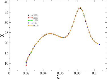
Figure 1: (Color online) Susceptibility against infection rate for SIS model on a single network with different fraction of initially infected vertices, which are randomly distributed in the network. The network parameters are $\gamma=3.5$, $k_{0}=3$ and $N=10^{6}$.

Reference Boguñá et al. (2013) claimed that the QS method is unreliable for networks with degree exponents $\gamma>3$ and proposed a new simulation strategy, which is referred here as lifespan simulation method. In order to draw a comparison with the QS method, we implemented the lifespan method exactly as in Ref. Boguñá et al. (2013): The simulation starts with a single infected vertex located at the most connected vertex of the network and stops when either the system visits the absorbing state or 50% of all vertices (the epidemic coverage) were infected at least once along the simulation. The duration of the epidemic outbreak is computed and only runs that visited the absorbing state are used to compute the average lifespan since those that reached 50% of coverage are assumed as having an infinite lifespan. The number of runs varies from $10^{3}$, for largest $N$ and $\lambda$, to $10^{6}$, for the smallest $\lambda$.

We applied both methods to the SIS model on UCM networks with $\gamma=3.50$, minimum degree $k_{0}=3$, and upper cutoff $k_{max}=\langle{k_{max}}\rangle$, in which $\langle{k_{max}}\rangle$ is the analytically determined mean value of the most connected vertex $k_{max}$ of a random degree sequence with distribution $P(k)$ without upper bounds, to compare with the results of Ref. Boguñá et al. (2013). The constraint $k_{max}=\langle{k_{max}}\rangle$ avoids fluctuations in the most connected vertex and, consequently, in the largest eigenvalue of the adjacency matrix and is useful for comparisons with the QMF theory Ferreira et al. (2012). We remark that the constraint $k_{max}=\langle{k_{max}}\rangle$ is only used in this comparison.

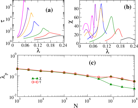
Figure 2: (Color online) Numerical determination of the thresholds for the SIS model on UCM networks with $\gamma=3.50$, $k_{0}=3$ and $k_{max}=\langle{k_{max}}\rangle$ for network sizes $N=10^{3},10^{4},10^{5},10^{6},10^{7},3\times 10^{7}$, and $10^{8}$, increasing from the right. A same network sample for each size was used in both methods. Both (a) lifespan calculated using the method of Ref. Boguñá et al. (2013) and (b) susceptibility via QS method are shown in the top panels. (c) Peak positions as functions of the network size estimated with both methods.

Figures 2(a) and (b) show the lifespan and susceptibility against infection rate for networks of different sizes. The peak positions against network size are compared in Fig 2(c). As can be clearly seen, the right susceptibility peaks are very close to the lifespan ones showing that the susceptibility method is able to capture the same transitions as the lifespan method does but going beyond as discussed in the rest of the paper. It is worth noticing that if larger values of $\lambda$ are simulated, other peaks will emerge in susceptibility curves even using the cutoff $k\leq\langle k_{max}\rangle$. These multiple peaks were not reported in previous works dealing with the same network model Ferreira et al. (2012); Mata and Ferreira (2013); Boguñá et al. (2013).

Moreover, a lifespan is also obtained in the QS method as de Oliveira and Dickman (2005)

$$\tau_{qs}=\frac{1}{\bar{P}(1)}.$$ (2)

We checked that the lifespans obtained in the QS method and those of Ref. Boguñá et al. (2013) diverge around the same threshold; the basic difference is that the former is “infinite” above the threshold whereas the latter remains finite.

In a partial summary, we verified that the lifespan method predicts an epidemic threshold when an activity survives for long times, but there is no guaranty that it is necessarily an endemic phase (see appendix A for a concrete counter-example). On the other hand, the QS analysis is able to simultaneously determine transitions involving endemic as well as localized states and the one involving a diverging lifespan is resolved using Eq. (2). So, we conclude that lifespan method must not be used alone in systems with multiple transitions since it captures the first transition with a long-term activity.

III Numerical Results

Two-peaks on susceptibility against infection rate for SIS were firstly reported in Ref. Ferreira et al. (2012), which focused on the analysis of the peak at low $\lambda$ and showed that it is well described by the QMF theory (see also Ref. Mata and Ferreira (2013)) but did not realize that the peak at higher $\lambda$ is the one associated to a diverging lifespan (Fig. 2). However, depending on the network realization, the susceptibility curves can exhibit much more complex behaviors with multiple peaks for values of $\lambda$ larger than those reported in Refs. Ferreira et al. (2012); Mata and Ferreira (2013). These complex behaviors become very frequent for large networks. From now on, we scrutinize such a complex behavior to unveil its origin and implications to the epidemic activity.

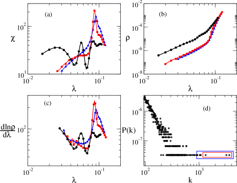
Figure 3: (Color online) (a) Susceptibility, (b) stationary density and (c) its logarithmic derivative versus infection rate for a SF network with $3\times 10^{7}$ vertices, degree exponent $\gamma=3.5$, minimum degree $k_{0}=3$ and $k_{max}$ unconstrained. The degree distribution is shown in panel (d). Different immunization strategies are shown: Black circles represent no immunization; red squares represent the immunization of three largest outliers (inner box in panel (d)); blue triangles represent the immunization of eight most connected vertices (outer box in panel (d)).

Figure 3(a) shows a typical susceptibility curve (black) exhibiting such a complex behavior for an UCM network. The degree distribution is shown in Fig. 3(d). Multiple peaks are observed only if the degree distribution exhibits a few large gaps, in particular in the tails. These few vertices with degree $k\gtrsim\langle{k_{max}}\rangle$ are hereafter called outliers. Notice that the multiple peaks are not detected by the lifespan simulation method Boguñá et al. (2013). The role played by outliers is evidenced by their immunizations as illustrated in Fig. 3. For instance, the immunization of the three most connected vertices is sufficient to destroy two peaks and to enhance others. The stationary density varies abruptly close to the thresholds determined via susceptibility peaks, Figs. 3(b) and (c), which is an evidence of the singular behavior of the order parameter $\rho$.

The presence of gaps is a characteristics of large degree sequences with a power law distribution. The statistical representativity of specific properties of a finite set of networks, generated under the same conditions, in relation to the entire ensemble is a complex issue Del Genio et al. (2010), but the existence of gaps can be understood with a simple non-rigorous reasoning. Using extreme value theory one can show that the most connected vertex has an average $\langle{k_{max}}\rangle\sim N^{1/(\gamma-1)}$ Boguñá et al. (2009). However, this mean value is not representative of the highest degree since the dispersion $\sigma_{max}=\sqrt{\langle{k_{max}^{2}}\rangle-\langle{k_{max}}\rangle^{2}}$ diverges as $\sigma_{max}\sim N^{1/(\gamma-1)}$ for $\gamma>3$. Outliers should behave in this same way and therefore we expect larger dispersion in outlier connectivity as network size increases.

It is interesting to observe that while the peaks at small $\lambda$ can or not appear depending on the presence of outliers and gaps, the rightmost one essentially does not change its position from a network realization to another, such that it should depend on network properties representative of the entire ensemble of networks with a specified set of parameters. Indeed, later we will see that the behavior of the rightmost peak is qualitatively described by the HMF threshold which depends only on $\langle{k^{2}}\rangle$ and $\langle{k}\rangle$.

A deeper physical explanation for the multiple peaks can be extracted using another order parameter in the QS state, the participation ratio (PR), defined as

$$\Phi=\frac{1}{N}\frac{(\sum_{i}\rho_{i})^{2}}{\sum_{i}\rho_{i}^{2}},$$ (3)

where $\rho_{i}$ is the probability that the vertex $i$ is infected in the stationary state. The inverse of the PR is a standard measure for localization/delocalization of states in condensed matter Bell and Dean (1970) and has been applied to statistical physics problems Plerou et al. (1999) including epidemic spreading on networks Goltsev et al. (2012); Barthélemy et al. (2004); Ódor (2013). The limiting cases of totally delocalized ($\rho_{i}=\rho$ $\forall~{}i$) and localized ($\rho_{i}=\rho\delta_{i,0}$ where 0 is the vertex where localization occurs) states are $\Phi=1$ and $\Phi=1/N$, respectively.

The PR as a function of the infection rate is shown in Fig. 4. The PR is an estimate of the fraction of vertices that effectively contribute to the present epidemic activity. Thus, the multiple transitions are related to the rapid delocalization processes of the epidemics as $\lambda$ increases, hallmarked by the singular behavior of $\Phi$ around distinct values of $\lambda$. When the PR corresponds to a finite fraction of the network in an active phase one has an authentic endemic state, since a finite fraction of nodes has a non-vanishing probability of being infected at the same time.

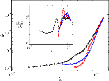
Figure 4: (Color online) Main: PR as a function of the infection rate for the same network and immunization strategies as in Fig. 3. Symbols as in Fig. 3. Inset: Logarithmic derivative of the PR as a function of the infection rate.

The logarithmic derivative of the PR exhibits several peaks in analogy to susceptibility peaks, as shown in the inset of Fig. 4. Indeed, PR can be seen as a susceptibility but from an origin different of $\chi$. The latter is a measure of stochastic fluctuations of the order parameter (density of infected vertices) whereas the former is measure of stationary spatial fluctuations that make sense only for heterogeneous substrates.

The PR against network size for a fixed distance to either $\lambda_{p}^{ls}$ (the threshold marking the lifespan divergence) and $\lambda_{p}^{right}$ (the threshold referent to the rightmost peak observed for susceptibility) are shown in Fig. 5(a). In the presented size range, the PR decays as a power law for a fixed distance to the lifespan peaks. Analogous results are obtained for $\bar{\rho}$ vs $N$ curves (see Fig. 5(b)). The power regressions yield approximately $\Phi\sim N^{-0.8}$ and $N^{-1}$ for $\gamma=3.5$ and 4, respectively, $\rho\sim N^{-0.8}$ for both $\gamma=3.5$ and 4. These decays constitute a strong evidence for epidemics localization at $\lambda\gtrsim\lambda_{p}^{ls}$ whereas the constant dependence on $N$ observed for $\lambda\gtrsim\lambda_{p}^{right}$ represents an endemic phase.

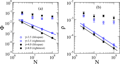
Figure 5: (Color online) (a) PR against size for a fixed distance $\lambda-\lambda_{p}=0.012$ to either lifespan (circles) and rightmost (squares) peaks. (b) The same analysis of panel (a) for QS density. Lines are power regressions. At least 10 network samples were used to perform averages for $\lambda>\lambda_{p}^{right}$ (top curves) and at least 20 for $\lambda_{p}^{ls}<\lambda<\lambda_{p}^{right}$ (bottom curves).

Figure 6 shows the positions $\lambda_{p}^{left}$ (the leftmost peak), $\lambda_{p}^{right}$ and $\lambda_{p}^{ls}$ against the network size. One can see that $\lambda_{p}^{right}$ reaches a constant value for large $N$ whereas the other ones neatly decays with $N$. In a nutshell, our results show that the case $\gamma>3$ may concomitantly exhibit transitions predicted by three competing mean-field theories: (i) At $\lambda=\lambda_{p}^{left}$, one has a transition to an epidemics highly concentrated at the star subgraph containing the most connected vertex and its nearest neighbors. The threshold dependence on size is very well described by QMF theories Castellano and Pastor-Satorras (2010); Ferreira et al. (2012); Mata and Ferreira (2013). (ii) At $\lambda=\lambda_{p}^{ls}$, a transition with a threshold described by the BCPS theory Boguñá et al. (2013) is observed but, our numerics indicate that it is not endemic since PR and $\rho$ decays with $N$ above this threshold. Notice that the threshold $\lambda_{p}^{ls}$ decays with $N$ much slower than $\lambda_{p}^{left}$. This interval is characterized by the mutual activation of stars sub-graphs centered on the outliers by means of reinfection mechanism proposed in the BCSP theory Boguñá et al. (2013). (iii) For $\lambda=\lambda_{p}^{right}$, a transition involving an authentic endemic phase with a finite threshold is observed as formerly, and now surprisingly, predicted by the HMF theory Pastor-Satorras and Vespignani (2001a); *Pastor01b. Here, the bulk of the network acts collectively in the epidemic spreading through the whole network characterizing a real phase transition.

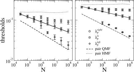
Figure 6: Thresholds for SIS dynamics on SF networks with degree exponents $\gamma=3.5$ (left) and $\gamma=4.0$ (right). The results predicted by pair QMF Mata and Ferreira (2013) and pair HMF Mata et al. (2014) theories are shown as dashed and doted lines, respectively. Solid lines are power law regressions. Averages were done over at least 5 samples for the statistics of the rightmost peaks and at least 20 samples for lifespan and leftmost peaks.

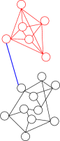
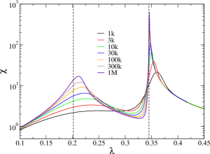
Figure 7: Left: Schematics of a double random regular network (DRRN). Right: Susceptibility against infection rate for DRRNs with using $m_{1}=4$, $m_{2}=6$, $\alpha=1/2$ and different sizes. Dashed lines are thresholds predicted for DRRNs.

The co-existence of localized and endemic transitions in a same network can be explained in a double random regular network (DRRN), Fig. 7. These networks are formed by two random regular networks (RRNs) of sizes $N_{1}$ and $N_{2}=N_{1}^{\alpha}$ ($\alpha<1\Rightarrow N_{2}/N_{1}\rightarrow 0$ in the thermodynamical limit) and degree $m_{1}$ and $m_{2}$, respectively, connected by a single edge. The DRRN has two epidemic thresholds corresponding to the activations of single RRNs. Choosing $m_{1}=4$ and $m_{2}=6$, the thresholds determined for single RRNs are $\lambda_{c}^{(1)}=0.31452$ ($m_{1}=4$, present work) and $\lambda_{c}^{(2)}=0.2026$ ($m_{2}=6$ Ferreira and Ferreira (2013)). By construction, the former involves an endemic and latter a localized transition since the smaller RRN constitutes itself a vanishing fraction of the whole network. Figure 7 shows the susceptibility plots for $\alpha=0.5$ with peaks converging exactly to the expected thresholds. The threshold obtained via lifespan method, which is in principle fitted by the BCPS theory, converges to the localized one (see appendix A for additional data and discussions). This network model can be generalized to produce an arbitrary number of transitions providing a clearer analogy with multiple transitions observed for random networks with $\gamma>3$.

An additional property can be derived for random networks with $\gamma>3$: outliers have negligibly low probability to be connected to each other. Due to the absence of degree correlation, the probability that a vertex of degree $k$ is connected to an outlier of degree $k_{out}$ is given by $P(k|k_{out})=kP(k)/\langle{k}\rangle$ Boguñá et al. (2004) irrespective of the outlier’s degree. Therefore the probability that an outlier is connected to other outlier is given by

$$P_{out}\simeq\int_{k\gtrsim\langle{k_{max}}\rangle}P(k|k_{out})dk\sim\langle{k_{max}}\rangle^{-\gamma+2},$$

which goes to zero for large networks permitting the formation of non directly connected domains centered on the outliers. This conclusion can be obtained rigorously using hidden variable formalism Serrano et al. (2011). We have now a simple physical explanation for multiple thresholds and its connection with the lifespan simulation method: The core containing the outliers plus its nearest neighbors form a subgraph with $N_{2}\sim\sum_{k>\langle{k_{max}}\rangle}NP(k)k\sim N^{1/(\gamma-1)}\ll N$. This domain size diverges as network increases and is able to sustain a long-term epidemic activity, but still represents a vanishing fraction of the whole network. Above the activation of this domain but still below the endemic phase, the epidemics is eventually transmitted to any other vertex of the network due to the small-world property, but this activity dies out quickly outside this core since there the process is locally sub-critical. However, all network vertices will be infected for some while since the active central core acts as a reservoir of infectiousness to the rest of the network.

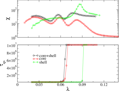
Figure 8: (Color online) Susceptibility (top) and QS lifespan (bottom) against infection rate for SIS dynamics on a network with $N=3\times 10^{7}$, $k_{0}=3$ and degree exponent $\gamma=3.50$ restricted to different domains (see text for definitions). The lifespan is considered infinite if greater than the averaging time $t_{av}=10^{7}$.

Our conjecture is confirmed in Fig. 8 where SIS dynamics in a large network ($N=3\times 10^{7}$ vertices) is compared with the dynamics restricted to either its core of outliers (7 most connected vertices) plus their nearest neighbors ($\approx 13200$ vertices) or to its outer shell excluding the core. The multiple peaks for the core are observed approximately at the same places as those for the whole network but the outer shell exhibits a single peak around $\lambda_{p}^{right}$. However, the lifespan determined via QS method (see section II) diverges at $\lambda\approx\lambda_{p}^{ls}$ for both core and whole network whereas the divergence coincides with $\lambda_{p}^{right}$ for the outer shell.

We also analyzed the lifespan using the QS method, Eq. (2), for a fixed distance to both leftmost and lifespan peaks. For the investigated size range $N<10^{8}$, the lifespan values are relatively short ($<10^{2}$) and increase algebraically with system size in the interval $\lambda_{p}^{left}<\lambda<\lambda_{p}^{ls}$ while long and exponentially diverging lifespans, granting long-term activity for large networks Ganesh et al. (2005), are obtained for $\lambda_{p}^{ls}<\lambda<\lambda_{p}^{right}$. The algebraic dependence for the former case is almost certainly a finite-size effect. We calculated the lifespan for $\lambda_{p}^{left}<\lambda<\lambda_{p}^{ls}$ for the SIS model on star graphs with $k$ leaves and an algebraic growth of the lifespan with $N$ is also obtained for $k<2000$ which coincides with the range size of typical star subgraphs obtained for UCM networks investigated here. However, a crossover to an exponential growth is obtained for larger star graphs ($k>10^{4}$) showing that this structure is itself able to sustain alone a long-term epidemic activity. So, if one could simulate SIS model on much larger UCM networks ($N>10^{12}$) the threshold $\lambda_{p}^{left}$ would define a transition to a localized but long-term epidemics and the lifespan method would detect the transition given by the QMF theory.

Outliers play a central role even not being able to produce separately a genuine endemic phase where the whole network has a non-vanishing probability of being infected. To highlight such a role, we introduce a hard cutoff in the degree distribution as $k_{max}=k_{0}N^{0.75/(\gamma-1)}$, which suppresses the emergence of outliers as shown in Fig. 9(a). This choice is because random networks without a rigid upper bound have a highly fluctuating natural cutoff, as discussed above. Fig. 9(b) compares the QS density for rigid and natural cutoffs. The infectiousness for $\lambda<\lambda_{c}^{endemic}$ is highly reduced in the absence of outliers. The susceptibility no longer exhibits multiple peaks for a hard cutoff, as can be seen in Fig. 10(a), confirming the existence of a single transition. Also, the thresholds for hard cutoff networks are quite close to $\lambda_{p}^{right}$ obtained with the natural cutoff, as shown in Fig. 10(b). Such an observation is in agreement with the HMF theory where the thresholds for $\gamma>3$ are asymptotically independent of how $k_{c}$ diverges Pastor-Satorras and Vespignani (2001a); *Pastor01b; Mata et al. (2014).

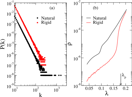
Figure 9: (Color online) (a) The tail of the degree distributions for networks with $\gamma=4$, $k_{0}=3$, and $N=10^{8}$ vertices and either rigid or natural cutoff. The curve for rigid cutoff was shifted to enhance visibility. (b) QS density against infection rate for a network degree exponent $\gamma=4.0$ using different cutoffs.

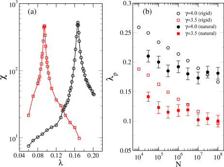
Figure 10: (Color online) (a) Susceptibility curves for two networks with rigid cutoff, $k_{0}=3$, $N=10^{8}$ vertices and different degree exponent (symbols are the same used in panel (b)). (b) Threshold against system size for rigid and natural cutoffs. The averages were done over at least 6 samples for rigid cutoff but error bars are smaller than symbols. Averages for natural cutoffs are the same as in Fig. 6.

IV Conclusions

In summary, we thoroughly simulated the dynamics of the SIS epidemic model on complex networks with power law degree distributions with exponent $\gamma>3$, for which conflicting theories discussing the existence or not of a finite epidemic threshold for the endemic phase have recently been proposed Castellano and Pastor-Satorras (2010); Goltsev et al. (2012); Boguñá et al. (2013); Lee et al. (2013a). We show that the SIS dynamics can indeed exhibit several transitions associated to different epidemiological scenarios. Our simulations support a picture where the threshold obtained recently in the BCPS mean-field theory Boguñá et al. (2013) represents a transition to localized epidemics in random networks wih $\gamma>3$ and that the transition to an authentic endemic state, in which a finite fraction of network is infected, possibly occurs at a finite threshold as formerly and now surprisingly foreseen by the HMF theory Pastor-Satorras and Vespignani (2001a); *Pastor01b. The multiple transitions are associated to large gaps in the degree distribution with a few outliers, which permits the formation of non-directly connected domains of activity centered on these outliers. If the number of hubs is large, as in the case of SF networks with $\gamma<3$, every vertex of the network is “near” to some hub and the activation of hubs implies in the activation of the whole network, as previously reported in Ferreira et al. (2012); Mata and Ferreira (2013). Our finds are consistent with the conjecture proposed by Lee et al. Lee et al. (2013a) since the lifespans of independent domains involving outliers grow exponentially fast with the domain sizes implying that long-term epidemic activity is possible even in non-endemic phase. Our finds also do not rule out the mean-field analysis of Ref. Goltsev et al. (2012). The intermediary transitions can be associated to distinct localized eigenvectors that are centered on the outliers while the endemic threshold involves a delocalized eigenvector with a finite eigenvalue.

Our results are in consonance with a recent line of investigation, in which the topological disorder in networks with heterogeneous degree distribution may produce rare regions and Griffiths phases leading to anomalous behaviors in the subcritical phase Lee et al. (2013a); Muñoz et al. (2010); Buono et al. (2013); Ódor (2013). Such anomaly is characterized by localized activity that survives for long times, even though the network is macroscopically absorbing. Very recently, the possibility of rare regions effects from pure topological disorder in the SIS dynamics on unweighted SF networks as well as multiple transitions were suggested in Ref. Ódor (2014). Our results may, thus, be a fingerprint of GPs. However, more detailed analyses are demanded for a conclusive relation. Also, very recently, multiple phase transitions were found in percolation problems on SF networks with high clustering Colomer-de Simón and Boguñá (2014) and on networks of networks Bianconi and Dorogovtsev (2014). In both cases transitions were hallmarked by multiple singular points in the order parameter in analogy with our results for epidemics.

Our final overview is that apparently competing mean-field theories Pastor-Satorras and Vespignani (2001a); *Pastor01b; Castellano and Pastor-Satorras (2010); Goltsev et al. (2012); Boguñá et al. (2013); Lee et al. (2013a) can be considered, in fact, complementary, describing distinct transitions that may concomitantly emerge depending on the network structure. In particular, the transitions involving localized phases, as possibly the one predicted by the BCPS theory Boguñá et al. (2013), are not negligible since they become long-term and an epidemic outbreak may eventually visit a finite fraction of the network. This peculiar result is unthinkable for other substrates rather than complex networks sharing the small-world and scale-free properties. Actually, it is well known that some computer viruses can survive for long periods (years) in a very low density (below $10^{-4}$) Pastor-Satorras and Vespignani (2004), exemplifying the importance of metastable non-endemic states. Our numerical results call for general theoretical approaches to describe in an unified framework the multiple transitions of the SIS dynamics on SF networks.

Appendix A Quasistationary versus lifespan methods

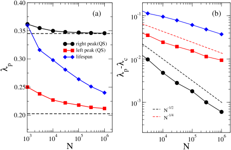
Figure 11: (Color online) Threshold analysis for DRRN with $\alpha=1/2$, $m_{1}=4$, and $m_{2}=6$. (a) The thresholds estimated as the peaks in the susceptibility or lifespan curves. The dashed lines are thresholds obtained on single RRNs with the respective $m_{i}$. (b) Difference between peaks and the thresholds for single RRNs with $m=4$ (lifespan and left susceptibility peaks) or $m=6$ (right susceptibility peak).

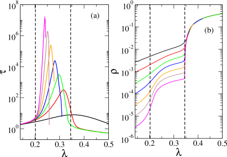
Figure 12: (Color online) (a) The lifespan according Ref. Boguñá et al. (2013) and (b) the QS density of infected vertices against infection rate for SIS model on DRRNs with $\alpha=1/2$, $m_{1}=4$, $m_{2}=6$, $N_{1}=10^{3},~{}3\times 10^{3},~{}10^{4},~{}3\times 10^{4},~{}10^{5},~{}3\times 10^{5},$ and $10^{6}$ (increasing to left or bottom in (a) or (b), respectively). Dashed vertical lines indicate the activation thresholds in each sub-graph.

Lets show that the QS method succeeds whereas lifespan method fails in predicting the endemic phase for a DRRN (Fig. 7). The susceptibility peaks in Fig. 7 clearly converge to the respective thresholds of single RRNs as highlighted in Fig. 11(a) and (b). Notice that the mean-field theory for the finite-size scaling of the contact process, which in the case of strictly homogeneous networks is exactly the same as SIS model with a rescaled infection rate $\lambda/m$, predicts that the threshold approaches its asymptotic values as $\lambda_{p}-\lambda_{c}\sim S^{-1/2}$, where $S$ is the graph size Mata et al. (2014). So, the endemic threshold is expected to scale as $\lambda_{p}-\lambda_{c}^{(1)}\sim N_{1}^{-1/2}\sim N^{-1/2}$ and the localized one as $\lambda_{p}-\lambda_{c}^{(2)}\sim N_{2}^{-1/2}\sim N^{-\alpha/2}$. These power-laws are confirmed in Fig. 11(b). The lifespan curves, obtained using as initial condition only the most connected vertex infected (the one connecting sub-graphs), have single peaks that converge to the threshold corresponding to a localized epidemic and interestingly following the same scaling law as the left QS peak as shown in Figs. 11 and 12(a). The central point here is that the lifespan method detected the first threshold where the absorbing state becomes globally unstable (an exponentially long-term activity) that, in this case, is not the endemic one as shown in Fig. 12(b), in which the QS density is shown as a function of the infection rate.

It is worth noticing that the QS simulations around the peaks are orders of magnitude computationally more efficient than the lifespan method.

References

- Dorogovtsev et al. (2008) S. N. Dorogovtsev, A. V. Goltsev, and J. F. F. Mendes, Rev. Mod. Phys. 80, 1275 (2008).
- Albert et al. (2000) R. Albert, H. Jeong, and A.-L. Barabási, Nature 406, 378 (2000).
- Pastor-Satorras and Vespignani (2001a) R. Pastor-Satorras and A. Vespignani, Phys. Rev. Lett. 86, 3200 (2001a).
- Pastor-Satorras and Vespignani (2001b) R. Pastor-Satorras and A. Vespignani, Phys. Rev. E 63, 066117 (2001b).
- Dorogovtsev et al. (2002) S. N. Dorogovtsev, A. V. Goltsev, and J. F. F. Mendes, Phys. Rev. E 66, 016104 (2002).
- Henkel et al. (2008) M. Henkel, H. Hinrichsen, S. Lübeck, and M. Pleimling, Non-equilibrium phase transitions, Vol. 1 (Springer, Dordrecht, Netherlands, 2008).
- Castellano and Pastor-Satorras (2008) C. Castellano and R. Pastor-Satorras, Phys. Rev. Lett. 100, 148701 (2008).
- Hong et al. (2007) H. Hong, M. Ha, and H. Park, Phys. Rev. Lett. 98, 258701 (2007).
- Juhász et al. (2012) R. Juhász, G. Ódor, C. Castellano, and M. A. Muñoz, Phys. Rev. E 85, 066125 (2012).
- Mata et al. (2014) A. S. Mata, R. S. Ferreira, and S. C. Ferreira, N. J. Phys. 16, 053006 (2014).
- Ferreira et al. (2011) S. C. Ferreira, R. S. Ferreira, and R. Pastor-Satorras, Phys. Rev. E 83, 066113 (2011).
- Castellano and Pastor-Satorras (2010) C. Castellano and R. Pastor-Satorras, Phys. Rev. Lett. 105, 218701 (2010).
- Goltsev et al. (2012) A. V. Goltsev, S. N. Dorogovtsev, J. G. Oliveira, and J. F. F. Mendes, Phys. Rev. Lett. 109, 128702 (2012).
- Ferreira et al. (2012) S. C. Ferreira, C. Castellano, and R. Pastor-Satorras, Phys. Rev. E 86, 041125 (2012).
- Boguñá et al. (2013) M. Boguñá, C. Castellano, and R. Pastor-Satorras, Phys. Rev. Lett. 111, 068701 (2013).
- Lee et al. (2013a) H. K. Lee, P.-S. Shim, and J. D. Noh, Phys. Rev. E 87, 062812 (2013a).
- Cator and Van Mieghem (2012) E. Cator and P. Van Mieghem, Phys. Rev. E 85, 056111 (2012).
- Mieghem (2012) P. V. Mieghem, Eur. Lett. 97, 48004 (2012).
- Chakrabarti et al. (2008) D. Chakrabarti, Y. Wang, C. Wang, J. Leskovec, and C. Faloutsos, ACM Trans. Inf. Syst. Secur. 10, 1 (2008).
- Mata and Ferreira (2013) A. S. Mata and S. C. Ferreira, Eur. Lett. 103, 48003 (2013).
- Ódor (2014) G. Ódor, Phys. Rev. E 90, 032110 (2014).
- Noest (1986) A. J. Noest, Phys. Rev. Lett. 57, 90 (1986).
- Vojta et al. (2009) T. Vojta, A. Farquhar, and J. Mast, Phys. Rev. E 79, 011111 (2009).
- Lee et al. (2013b) H. K. Lee, P.-S. Shim, and J. D. Noh, Preprint , ArXiv:1309.5367 (2013b).
- Boguñá et al. (2014) M. Boguñá, C. Castellano, and R. Pastor-Satorras, preprint arXiv:1403.7913 (2014).
- Gillespie (1976) D. T. Gillespie, J. Comput. Phys. 22, 403 (1976).
- de Oliveira and Dickman (2005) M. M. de Oliveira and R. Dickman, Phys. Rev. E 71, 016129 (2005).
- Dickman and Vidigal (2002) R. Dickman and R. Vidigal, J. Phys. A: Math. Gen. 35, 1147 (2002).
- Blanchet et al. (2014) J. Blanchet, P. Glynn, and S. Zheng, arXiv preprint arXiv:1401.0364 (2014).
- Newman (2010) M. Newman, Networks: An Introduction (Oxford University Press, Inc., New York, NY, USA, 2010).
- Watts and Strogatz (1998) D. J. Watts and S. H. Strogatz, Nature 393, 440 (1998).
- Ferreira and Ferreira (2013) R. S. Ferreira and S. C. Ferreira, Eur. Phys. J. B 86, 1 (2013).
- Catanzaro et al. (2005) M. Catanzaro, M. Boguñá, and R. Pastor-Satorras, Phys. Rev. E 71, 027103 (2005).
- Press et al. (2007) W. H. Press, S. A. Teukolsky, W. T. Vetterling, and B. P. Flannery, Numerical Recipes 3rd Edition: The Art of Scientific Computing, 3rd ed. (Cambridge University Press, New York, NY, USA, 2007).
- Van Mieghem and Cator (2012) P. Van Mieghem and E. Cator, Phys. Rev. E 86, 016116 (2012).
- (36) R. S. Sander and S. C. Fereira, in preparation .
- Del Genio et al. (2010) C. I. Del Genio, H. Kim, Z. Toroczkai, and K. E. Bassler, PLoS ONE 5, e10012 (2010).
- Boguñá et al. (2009) M. Boguñá, C. Castellano, and R. Pastor-Satorras, Phys. Rev. E 79, 036110 (2009).
- Bell and Dean (1970) R. J. Bell and P. Dean, Discuss. Faraday Soc. 50, 55 (1970).
- Plerou et al. (1999) V. Plerou, P. Gopikrishnan, B. Rosenow, L. A. Nunes Amaral, and H. E. Stanley, Phys. Rev. Lett. 83, 1471 (1999).
- Barthélemy et al. (2004) M. Barthélemy, A. Barrat, R. Pastor-Satorras, and A. Vespignani, Phys. Rev. Lett. 92, 178701 (2004).
- Ódor (2013) G. Ódor, Phys. Rev. E 88, 032109 (2013).
- Boguñá et al. (2004) M. Boguñá, R. Pastor-Satorras, and A. Vespignani, Eur. Phys. J. B 38, 205 (2004).
- Serrano et al. (2011) M. A. Serrano, D. Krioukov, and M. Boguñá, Phys. Rev. Lett. 106, 048701 (2011).
- Ganesh et al. (2005) A. Ganesh, L. Massoulié, and D. Towsley, in IEEE INFOCOM (2005) pp. 1455–1466.
- Muñoz et al. (2010) M. A. Muñoz, R. Juhász, C. Castellano, and G. Ódor, Phys. Rev. Lett. 105, 128701 (2010).
- Buono et al. (2013) C. Buono, F. Vazquez, P. A. Macri, and L. A. Braunstein, Phys. Rev. E 88, 022813 (2013).
- Colomer-de Simón and Boguñá (2014) P. Colomer-de Simón and M. Boguñá, Phys. Rev. X 4, 041020 (2014).
- Bianconi and Dorogovtsev (2014) G. Bianconi and S. N. Dorogovtsev, Phys. Rev. E 89, 062814 (2014).
- Pastor-Satorras and Vespignani (2004) R. Pastor-Satorras and A. Vespignani, Evolution and structure of the Internet: A statistical physics approach (Cambridge University Press, Cambridge, 2004).