QMUL-PH-14-03

WITS-CTP-131

CFT₄ as $SO(4,2)$-invariant TFT₂

Robert de Mello Koch ^a, and Sanjaye Ramgoolam ^b,

^a National Institute for Theoretical Physics ,

School of Physics and Centre for Theoretical Physics

University of the Witwatersrand, Wits, 2050,

South Africa

^b Centre for Research in String Theory, School of Physics and Astronomy,

Queen Mary University of London,

Mile End Road, London E1 4NS, UK

ABSTRACT

We show that correlators of local operators in four dimensional free scalar field theory can be expressed in terms of amplitudes in a two dimensional topological field theory (TFT₂). We describe the state space of the TFT₂, which has $SO(4,2)$ as a global symmetry, and includes both positive and negative energy representations. Invariant amplitudes in the TFT₂ correspond to surfaces interpolating from multiple circles to the vacuum. They are constructed from $SO(4,2)$ invariant linear maps from the tensor product of the state spaces to complex numbers. When appropriate states labeled by 4D-spacetime coordinates are inserted at the circles, the TFT₂ amplitudes become correlators of the four-dimensional CFT₄. The TFT₂ structure includes an associative algebra, related to crossing in the 4D-CFT, with a non-degenerate pairing related to the CFT inner product in the CFT₄. In the free-field case, the TFT₂/CFT₄ correspondence can largely be understood as realization of free quantum field theory as a categorified form of classical invariant theory for appropriate $SO(4,2)$ representations. We discuss the prospects of going beyond free fields in this framework.

1 Introduction

In this paper we develop a new perspective on correlators of four dimensional conformal field theory using two dimensional topological field theory. We are primarily concerned with the correlators of local operators in CFT₄ on $\mathbb{R}^{3,1}$ (or the Wick-rotated $\mathbb{R}^{4}$), where the space of states forms representations of the conformal group $SO(4,2)$. The explicit calculations in the paper will start from the simplest CFT₄, namely the free scalar field. We will outline how elements of the discussion generalize in various related free theories, and we will also see that many key elements in the discussion would be sensible for interacting theories. The symmetry $SO(4,2)$ plays the role of a global symmetry in the TFT₂.

The space of local operators of the CFT₄ will determine the state space of the TFT₂. In a TFT₂, we associate a state space $\mathcal{W}$ to a circle, and tensor products $\mathcal{W}^{\otimes k}$ to a disjoint union of $k$ circles. In $G$-invariant TFT₂, the state space is a linear representation of $G$. Here the state space $\mathcal{W}$ is a linear representation of $G=SO(4,2)$. TFT₂ associates, to an interpolating surface (cobordism) from $k$ circles to the vacuum, an $SO(4,2)$ invariant multi-linear map from $\mathcal{W}^{\otimes k}$ to complex numbers. For the case of the free scalar field, we will specify this map explicitly. There are two basic ingredients that go into this map. One is the fact that the 2-point function of the elementary field $\varphi$ of scalar field theory can be viewed as a generator for the matrix elements of the $SO(4,2)$ invariant map from $V_{+}\otimes V_{-}\rightarrow\mathbb{C}$. Here $V_{+}$ is the basic positive energy (lowest weight) representation of $SO(4,2)$ formed by $\varphi$ and its derivatives, while $V_{-}$ is the dual negative energy (highest weight) representation. The other ingredient that goes in the construction of the map from $\mathcal{W}^{\otimes k}\rightarrow\mathbb{C}$ is the combinatorics of Wick contractions. Using this invariant map, we can compute the $k$-point correlation functions of arbitrary composite operators. For the general background on TFT₂, including careful definition of orientations, of ingoing versus outgoing boundaries and of cobordisms and their equivalences, we found [1] to be a very useful reference.

Section 2 starts with the motivations from AdS/CFT leading to this work. It has recently been found that the combinatoric part of extremal correlators, notably three-point functions, of half-BPS operators can be expressed in terms of 2d TFTs built from lattice gauge theories where permutation groups play the role of gauge groups [2, 3, 4, 5, 6]. These belong to the class of theories considered by Dijkgraaf-Witten [7], and form examples of TFTs obeying the axioms stated by Atiyah [8]. This naturally raises the question of whether the full spacetime dependent correlators, not just the combinatoric part, can be understood using an appropriate TFT₂. Since the space-time dependences of three-point correlators are completely determined by the invariance of the theory under the conformal group $SO(4,2)$, the right TFT₂ has to have a global $SO(4,2)$ invariance. The notion of TFT₂ with a global $G$-invariance has been explained in [9]. One subtlety we have to deal with is that standard TFT₂’s have finite dimensional state spaces. This requirement of finite dimensionality follows from the way the axioms are set up, and physically relates to the fact that the TFT₂’s have amplitudes corresponding to surfaces of arbitrary genus. To allow infinite dimensional state spaces, we restrict to genus zero surfaces, so we have a genus zero TFT₂, which involve a genus zero subset of the equations and algebraic structures entering finite TFT₂’s. We describe this genus zero subset of equations and corresponding geometry of two dimensional cobordisms. Key among these properties are the existence of a product, corresponding to the 3-holed sphere with two ingoing and one outgoing boundary. This product is associative. Another key property is the existence of a non-degenerate pairing $\mathcal{W}\otimes\mathcal{W}\rightarrow\mathbb{C}$, which has to be $SO(4,2)$ invariant. The student of perturbative QFT is familiar with the fact that zero-dimensional Gaussian integrals provide a brilliant toy model to learn about QFT. Here the Gaussian integration model is used to provide what is arguably the simplest example of TFT₂, having infinite dimensional state space, associativity and non-degeneracy.

Section 3 describes how the basic two-point function of the elementary scalar in free scalar quantum field theory is understood in terms of $SO(4,2)$ invariants. Let $V_{+}$ be the irreducible representation of $SO(4,2)$, with states of positive scaling dimensions (positive energy in radial quantization), consisting of the field $\varphi$ and its derivatives, with the equations of motion set to zero. $V_{-}$ is the conjugate representation. There is no $SO(4,2)$ invariant in the tensor product $V_{+}\otimes V_{+}$, but there is an $SO(4,2)$ invariant bilinear map $\hat{\eta}:V_{+}\otimes V_{-}\rightarrow\mathbb{C}$. $\hat{\eta}$ is extended to an invariant map from $\hat{\eta}:V\otimes V\rightarrow\mathbb{C}$, where $V=V_{+}\oplus V_{-}$. This bilinear invariant plays a crucial role, so we study some of its properties. We describe the invariant explicitly by exploiting $SU(2)\times SU(2)$ and $SL(2)$ subalgebras of $SO(4,2)$. The $SO(4,2)$ invariance is neatly expressed as a set of partial differential equations obeyed by the generator of matrix elements of $\hat{\eta}$. Some additional representation theoretic constructions are described, notably a map $\rho:V_{+}\rightarrow V_{-}$, which is related to an automorphism of the $so(4,2)$ Lie algebra. By using $\hat{\eta},\rho$, we can construct an inner product $g$ on $V_{+}$ and on $V_{-}$. The positivity of $g$ is related to unitarity of the CFT. The invariance of $\hat{\eta}$ is important in giving a TFT₂ interpretation of the 2-point function in terms of an $SO(4,2)$ invariant map. These ideas can be understood in a simple toy model. Consider the spin half representation of $SU(2)$, denoted $V_{1\over 2}$. A problem in classical invariant theory is to count the number of times the trivial (one-dimensional) representation $\mathbb{C}$ appears in the Clebsch-Gordan decomposition of various tensor powers. If we take $V_{1\over 2}\otimes V_{1\over 2}$ it appears once. A more refined question is to describe the form of this state, which is

$$|{1\over 2},{1\over 2}>\otimes|{1\over 2},-{1\over 2}>~{}-~{}|{1\over 2},-{1\over 2}>\otimes|{1\over 2},{1\over 2}>$$ (1.1)

We are using the usual notation for $SU(2)$ reps where states in an irrep are labeled by $|j,m>$ with $J_{3}=m$ and quadratic Casimir equal to $j(j+1)$. Now if we let $x_{1}^{2J_{3}}\otimes x_{2}^{2J_{3}}$ act on this invariant state, we get back the state with a factor.

$${x_{1}\over x_{2}}-{x_{2}\over x_{1}}$$ (1.2)

The equations (1.1) (1.2) are equivalent ways to describe the form of the invariant state in $V_{1\over 2}\otimes V_{1\over 2}$. In the application to the TFT₂ construction of CFT₄ correlators, these $x_{1},x_{2}$ are replaced by 2 spacetime coordinates, and we are describing the invariant representation $\mathbb{C}$ in $V_{+}\otimes V_{-}$. The precise description of the invariant state in this way is a refinement of the counting of invariants. In this sense, this is a categorification of invariant theory and the TFT₂ construction of free field correlators involves a categorification of invariant theory for certain representations of $SO(4,2)$.

Section 4 describes the state space $\mathcal{W}$ of the TFT₂ corresponding to the free field CFT₄. Loosely speaking $\mathcal{W}$ contains states corresponding to all the composite operators in free field theory. The slight surprise is that it is $V=V_{+}\oplus V_{-}$, rather than $V_{+}$ or $V_{-}$ alone which enters the construction of $\mathcal{W}$. This is related to the fact mentioned above that there is an $SO(4,2)$ invariant in $V_{+}\otimes V_{-}$ but not in $V_{+}\otimes V_{+}$, so a construction of CFT₄ correlators from $SO(4,2)$ invariants in TFT₂ has to involve both $V_{+}$ and $V_{-}$ in the construction of the TFT₂ state space. We have

$$\mathcal{W}=\bigoplus_{n=0}^{\infty}\mathcal{W}_{n}$$ (1.3)

$$\mathcal{W}_{n}=Sym(V^{\otimes n})$$ (1.4)

The $n=0$ subspace $\mathcal{W}_{0}=\mathbb{C}$. The $n$-fold symmetric product arises because of the bosonic statistics of the free scalar. TFT₂ involves assigning $SO(4,2)$ invariant maps to interpolating surfaces (cobordisms) from disjoint unions of circles to the vacuum. We describe such an invariant map from $\mathcal{W}^{\otimes k}\rightarrow\mathbb{C}$ for any $k\geq 0$. It is constructed from the basic invariant $\hat{\eta}$, several copies of which are tensored according to Wick contraction combinatorics of QFT. We identify the basic field as a linear superposition of states, labeled by position $x\in\mathbb{R}^{4}$, living in $V_{+}$ and $V_{-}$,

$$\Phi(x)=\Phi^{+}(x)+\Phi^{-}(x^{\prime})$$ (1.5)

with $x^{\prime}$ related to $x$ by inversion. Using tensor products of this field, we have states corresponding to composite fields living in $\mathcal{W}_{n}$ for all $n$. Choosing coordinates $x_{1},x_{2}\cdots x_{k}$ for the composite fields thus defined, using tensor products and applying the invariant map, we get arbitrary correlators of composite fields at non-coincident points.

In section 5 we focus attention on the 2-point functions of arbitrary composite operators, viewed from the TFT₂ perspective. This is the amplitude for two circles going to the vacuum, denoted $\eta:\mathcal{W}\otimes\mathcal{W}\rightarrow\mathbb{C}$. We show that the non-degeneracy equation is satisfied, i.e. there is an inverse $\tilde{\eta}$ of $\eta$. This equation corresponds to the fact that we can glue a cylinder with two incoming boundaries to one with two outgoing boundaries, along one boundary from each, to give a cylinder with one in and one out boundary (see Figure 2). There is no gluing along two boundaries to produce a torus, which would give infinity because of the infinite dimensionality of the state spaces. This restriction is clear at the level of equations, but subtle at the level of rigorous category theoretic axiomatics. These subtleties are discussed in Section 9. The approach we take in the bulk of the paper is to define TFT₂ in terms of this restricted set of genus zero equations.

In section 6, we discuss 3-point functions and the operator product expansion. The relation between the two is provided by the inverse of $\eta$ discussed in Section 5. The amplitude for 3 circles to vacuum is the 3-point function. The amplitude for 2-circles to one circle is the OPE. The amplitude for one circle to two is the co-product.

In section 7, we discuss crossing and associativity. We explicitly prove the crossing property of the 4-point amplitude of TFT₂. This is related, using the non-degeneracy condition, to associativity, and also to what is sometimes called the Frobenius equation or the nabla-delta equation.

Section 8 looks at a basic problem in free scalar field theory, which is the enumeration of primary fields according to $SO(4,2)$ representation and multiplicity. We find that TFT₂’s with infinite dimensional state spaces, of the kind described in Section 2, play a role in the counting and lead to explicit new results for the case of three primary fields. This shows that the notion of genus zero TFT₂’s, with infinite dimensional state spaces which we have identified, is integral to the architecture of CFTs - not just to the whole CFT, but also to how the whole CFT is assembled from simpler parts. We hope to return to this theme by considering the construction of primary fields in the future. This would be another application of the counting to construction philosophy which finds various applications in the study of BPS states, integrability of giant graviton fluctuations and quiver combinatorics [10, 11, 6]. It is worth elaborating on counting to construction in this free scalar field setting. In the context of a free $O(N)$ vector model, the decomposition of the tensor product of the singleton representation (associated with the free scalar field) with itself into irreducible representations, as decsribed in the Flato-Fronsdal theorem[12], is the kinematics underlying the higher spin holography[13, 14, 15]. The relevance of the tensor product of the singleton with itself follows from the fact that to form $O(N)$ singlets in the vector model, one has to contract a product of two scalars. In the case of the matrix model, since we can take the product of an arbitrary number of matrices and trace to get a scalar, we need a more general version of the Flato-Fronsdal theorem which considers the tensor product of an arbitrary number of singleton representations. The generalized theorem will play a central role in the kinematics underlying the holography of the free CFT. Section 8 represents a concrete framework within which this generalized Flato Fronsdal theorem can be tackled.

Section 9 discusses outstanding problems and future directions. In particular, Section 9.4 considers generalized free fields, where the irrep $V_{+}$ is replaced by a more general irrep of $SO(4,2)$. In this more general set-up, we can still construct an $SO(4,2)$ invariant TFT₂ as defined in section 2. However, there is an additional condition related to having a local stress tensor that is not satisfied in the case of generalized free fields. We outline how this additional stress tensor condition can be expressed in terms of the $SO(4,2)$-invariant TFT₂ data.

The TFT₂ construction we have developed with $SO(4,2)$ can be repeated after replacing $SO(4,2)$ with other groups. If we consider $SO(d,2)$, we can relate CFTs in $d$ dimensions to TFT₂. We can also consider a compact group $G$. This will give $G$-invariant TFT₂’s. A unique invariant map $\hat{\eta}:V\otimes V\rightarrow\mathbb{C}$ can be defined for any finite dimensional representation $V$ of $G$ which contains, with unit multiplicity, the trivial irrep in the tensor product decomposition $V\otimes V$. $V$ can be an irreducible representation if that irrep is self-dual, or it can be a direct sum of some irreducible representation $V_{+}$ with its dual $V_{-}$. We can define the state space

$$\mathcal{W}=\bigoplus_{n=0}^{\infty}Sym(V^{\otimes n})$$ (1.6)

The amplitudes $C_{A_{1},\cdots,A_{k}}$ can be defined using tensor products of the elementary $\hat{\eta}$ as in Section 4. Since the proofs of non-degeneracy in Section 5 and of associativity in Section 7 are purely combinatoric, they will continue to hold in this more general set-up. It would be interesting to investigate applications of this general construction and to find path integral constructions which give rise to these TFT₂’s.

It is worth noting here that connections between 4D quantum field theories and two dimensional topological field theories, in diverse incarnations, have been a fruitful area of research. Superconformal indices of 4D theories have been related to 2D TFT [16]. In such applications the 2D surface has a physical origin as the surface that a 6D theory has to be compactified on to arrive at the 4D theory. Another way to related 4D QFT to 2D TFT is to twist the 4D theory so it becomes topological and then consider the 4D theory on a product of Riemann surfaces [17]. It is instructive to compare the present construction with these precedents. We have a 4D theory, and we are looking at local correlators, with non-trivial spacetime dependences. There is no dimensional reduction and the 2D surface arises as a geometrical device to encode, via its cobordism equivalences, the crossing and non-degeneracy properties of the 4D conformal field theory. The spacetime coordinates of local operators have become labels of states in the state space $\mathcal{W}$ associated boundary circles of the 2D surface. This is somewhat like string theory where spacetime momenta become labels of vertex operators inserted at points on the worldsheet. The observables do not depend on worldsheet metric, because we integrate out the worldsheet metrics, hence the topological nature. In this sense, our construction has some analogies to the twistor string proposal for $\mathcal{N}=4$ SYM [18].

It is also useful to consider the results of the present work in light of the general phenomenon of dualities in string and field theory. For instance T-duality in string theory is constructive and, for toroidal backgrounds, technically very simple : it exchanges the momentum and winding modes of string excitations. At the same time it has a conceptually very important aspect : it exchanges small and large sizes. Strong-weak dualities allow the computation of the strongly coupled theory in terms of its weakly coupled dual, but in most cases the explicit construction of the map is not known. The present CFT₄/TFT₂ correspondence is constructive, so in this sense, more like T-duality than $S$-duality. The construction encodes both the structure of the local operator and the space-time coordinates in the choice of boundary data. The conceptually intriguing part is that the four space-time coordinates of local operators are simply labels of states at the boundaries of the surfaces in two dimensions. So space-time as a stage for propagating fields has disappeared in the TFT₂ picture. This can be viewed as a form of space-time emergence, admittedly only in the context of free CFT₄ at this stage, but this is a proof of principle that space-time emergence (as opposed to just emergence of space) is possible in the world of dualities.

2 Genus zero TFT₂ equations

2.1 Motivations and strategy

The approach to correlators of CFT₄ we develop here, is motivated by studies of extremal correlators of half-BPS operators in $\mathcal{N}=4$ super Yang Mills theory with $U(N)$ gauge group. The half-BPS states correspond to multi-traces of an $N\times N$ complex matrix $Z$. For every positive integer $n$, these are gauge invariant observables which can be constructed using permutations $\sigma\in S_{n}$

$$\mathcal{O}_{\sigma}(x)\equiv Z^{i_{1}}_{i_{\sigma(1)}}(x)\cdots Z^{i_{n}}_{i_{\sigma(n)}}(x)$$ (2.1)

The correlators can be written as [2, 3, 4, 5, 6]

$$\langle\mathcal{O}_{\sigma_{1}}(x_{1})\mathcal{O}_{\sigma_{2}}(x_{2})\rangle={1\over|x_{1}-x_{2}|^{2n}}\sum_{\sigma_{1}^{\prime}\in T_{1}}\sum_{\sigma_{2}^{\prime}\in T_{2}}\sum_{\sigma_{3}\in S_{n}}\delta(\sigma_{1}^{\prime}\sigma_{2}^{\prime}\sigma_{3})N^{C_{\sigma_{3}}}$$ (2.2)

$T_{1}$ is the conjugacy class of the permutation $\sigma_{1}$. $T_{2}$ is the conjugacy class of the permutation $\sigma_{2}$. $C_{\sigma_{3}}$ is the number of cycles in the permutation $\sigma_{3}$. The combinatoric part of the correlator is constructed from a quantity $Z_{{\rm{TFT}}_{2}(S_{n})}(T_{1},T_{2},T_{3})$ which is a function of 3 conjugacy classes

$$Z_{{\rm{TFT}}_{2}(S_{n})}(T_{1},T_{2},T_{3})=\sum_{\sigma_{1}^{\prime}\in T_{2}}\sum_{\sigma_{2}^{\prime}\in T_{2}}\sum_{\sigma_{3}^{\prime}\in T_{3}}\delta(\sigma_{1}^{\prime}\sigma_{2}^{\prime}\sigma_{3}^{\prime})$$ (2.3)

This 2D topological field theory is an example from the class of TFT₂’s associated with finite groups $H$ (here $S_{n}$), which were first discussed by Dijkgraaf and Witten [7]. For closed Riemann surfaces, this sums over homomorphisms from the fundamental group of the surface to the group $H$. For manifolds with boundary, we sum over homomorphisms subject to a condition that the boundary group elements are restricted to some conjugacy classes. In the above case, we have the partition function on a 3-holed sphere, with $T_{1},T_{2},T_{3}$ being the three specified conjugacy classes at the boundaries.

Given that the combinatoric part has an elegant TFT₂ description, it is natural to ask if the same is true for the space-time dependent part of the correlator 2.2. This is known to be determined by the conformal group $SO(4,2)$. The simplest set-up to investigate this question is to consider ordinary (non-matrix) free scalar field theory. The main result of this paper is to describe this as an $SO(4,2)$-invariant TFT₂. We return to matrix scalar field theories briefly in Section 9.3 and outline how the $SO(4,2)$ and $S_{n}$ appear in the TFT₂ description in that case.

A TFT₂ associates a vector space $\mathcal{W}$ to a circle and tensor products of $\mathcal{W}$ to disjoint unions of circles. Cobordisms are associated to homomorphisms between tensor products of the vector spaces. From a physical point of view, once we have chosen a basis, there is discrete data : structure constants $C_{ABC}$ and a bilinear pairing $\eta_{AB}$, which obey some consistency conditions. These consistency conditions correspond to equivalences between different ways to construct cobordisms. They include, importantly, a non-degeneracy condition and an associativity condition.

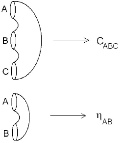
Figure 1: Basic building blocks and corresponding cobordisms

A variation on the above is associated to theories with global symmetry group $G$. Then $\mathcal{W}$ is a representation of $G$. The homomorphisms $\rho_{k_{1},k_{2}}:\mathcal{W}^{\otimes k_{1}}\rightarrow\mathcal{W}^{\otimes k_{2}}$ are $G$-equivariant, that is for any $g\in G$ the homomorphism and $g$ action commute $\rho_{k_{1},k_{2}}\circ g=g\circ\rho_{k_{1},k_{2}}$. So the vector space of states $\mathcal{W}$, whose basis states are labeled by $A,B,\cdots$, form a representation of a group $G$ (or its Lie algebra, when $G$ is a Lie group). The data $\eta_{AB}$ and $C_{ABC}$, are equivariant maps to the trivial representation $\mathbb{C}$, equivalently they are $G$-invariant maps. This notion of TFT₂ with global symmetry group $G$ is mentioned in [9] prior to developing TFT₂ with local $G$- symmetry, where the geometrical category involves circles with $G$-bundles and the cobordisms involve surfaces equipped with $G$-bundles.

2.2 Genus zero restriction and infinite dimensional state spaces

The standard axiomatic approach to TFT2 [1] requires the state spaces to be finite dimensional and includes finite amplitudes for surfaces of arbitrary genus. The first observation is that there is a well-defined subset, which we may call the genus zero subset of the TFT₂ equations, which do not involve summing over states in a (stringy) loop. These genus zero equations consist of a rich algebraic system including an associative product, non-degeneracy, unit, co-unit and co-product. These equations allow solutions involving infinite dimensional state spaces. So the $\eta_{AB},C_{ABC}$ are infinite dimensional arrays of numbers, with $A,B,\cdots$ running over an infinite discrete set of states. We will first write down some of these genus zero equations, and then show that there are simple non-trivial solutions, which we will call toy model solutions. The first toy model can be viewed as quantum field theory reduced to zero dimension and consists of Gaussian integration. A second toy model is related to $SU(2)$ tensor product multiplicities, which has applications in counting primary fields in CFT₄, as we will see in Section 8.

In subsequent sections we will show how these equations - with an appropriate choice of state space - provide a realization of free scalar field CFT₄ as a TFT₂. The equations obeyed by these structure constants have geometrical analogues in terms of equivalences of cobordisms (see [1] for the geometrical definitions and the equations, and a physics presentation in [19]). We write the key genus zero equations.

• Non-degeneracy : The 2-point function $\eta_{AB}$ has an inverse $\tilde{\eta}^{AB}$

  $$\eta_{AB}\tilde{\eta}^{BC}=\delta_{A}^{C}$$ (2.4)

  $\tilde{\eta}^{AB}$ corresponds to the cobordism from vacuum to two circles, while the identity on the RHS corresponds to the cylinder. Corresponding to (2.4) is the relation between cobordisms in Figure 2. In the case of finite dimensional state spaces, we also have $\eta_{AB}\tilde{\eta}^{BA}={\rm Dimension}$, which is closely related to non-degeneracy. This is a genus one cobordism from vacuum to vacuum which is excluded from our genus zero subset of equations.

• $G$ invariance : There invariance under a group $G$, which can be finite or a Lie group. In case of a Lie group, the invariance can be expressed in terms of the Lie algebra. For an element $\mathcal{L}$ in the Lie algebra of $G$, we have

  $$\mathcal{L}_{A}^{A^{\prime}}C_{A^{\prime}BC}+\mathcal{L}_{B}^{B^{\prime}}C_{AB^{\prime}C}+\mathcal{L}_{C}^{C^{\prime}}C_{ABC^{\prime}} = 0$$ (2.5)

  $$\mathcal{L}_{A}^{A^{\prime}}\eta_{A^{\prime}B}+\mathcal{L}_{B}^{B^{\prime}}\eta_{AB^{\prime}} = 0$$ (2.6)

  In our application to CFT₄, $G$ is $SO(4,2)$. In the toy model of Section 2.5, $G$ is trivial.

• Using the inverse $\tilde{\eta}$ of $\eta$, the 3-to-vacuum amplitude $C_{ABC}$ can be related to a 2-to-1 amplitude, which is the structure constant of an algebra.

  $$C_{AB}^{~{}~{}~{}D}=C_{ABC}\tilde{\eta}^{CD}$$ (2.7)

  In the applications to free field theory, this structure constant will be related to the operator product expansion, while $C_{ABC}$ will be related to 3-point correlators. As a relation between cobordisms, this is shown in Figure 3. Note that we might imagine associating one-dimensional pictures to such data, i.e. in this case a trivalent graph, and describing the equations in terms of relations between graphs. However a trivalent graph is not a manifold. Indeed in one dimension, cobordisms exist from one set of points to another only if the numbers of points are both even or both odd [1]. Here we keep as closely as possible to the standard topological field theory framework of cobordisms, hence two dimensions are naturally selected as the right geometrization of the equations.

• Using $\tilde{\eta}$ , we can also relate the 3-to-vacuum amplitude $C_{ABC}$ to a 1-to-2 amplitude, which is called a co-product.

  $$C_{A}^{~{}~{}DE}=C_{ABC}\tilde{\eta}^{BD}\tilde{\eta}^{CE}$$ (2.8)

  The figure corresponding to this is Figure 3.

• Symmetry Relations

  $$C_{ABC}=C_{BAC}=C_{ACB}$$ (2.9)

• Associativity :

  $$C_{AB}^{~{}~{}~{}E}C_{EC}^{~{}~{}~{}D}=C_{BC}^{~{}~{}~{}E}C_{EA}^{~{}~{}~{}D}$$ (2.10)

  This corresponds to the fact that the two different gluings shown in Figure 5 give equivalent cobordisms.

• Crossing :

  $$C_{AB}^{~{}~{}~{}E}C_{CD}^{~{}~{}~{}F}\eta_{EF}=C_{BC}^{~{}~{}~{}E}C_{AD}^{~{}~{}~{}F}\eta_{EF}$$ (2.11)

  Using the non-degeneracy equation, this is equivalent to associativity, which we elaborate on in Section 2.4. We also show there the equivalence to the Frobenius relation.

• $G$-invariance conditions for $\tilde{\eta}^{AB}$ and $C_{AB}^{~{}~{}~{}C}$ follow from the previous equations (2.5)

  $$\mathcal{L}^{A}_{A^{\prime}}\tilde{\eta}^{A^{\prime}B}+\mathcal{L}^{B}_{B^{\prime}}\tilde{\eta}^{AB^{\prime}}=0$$ (2.12)

  $$\mathcal{L}_{A}^{A^{\prime}}C_{A^{\prime}B}^{~{}~{}~{}~{}C}+\mathcal{L}_{B}^{B^{\prime}}C_{AB^{\prime}}^{~{}~{}~{}~{}C}-\mathcal{L}^{C}_{C^{\prime}}C_{AB}^{~{}~{}~{}~{}C^{\prime}}=0$$ (2.13)

• In the context of the TFT₂/CFT₄ construction in Section 3, we will use an automorphism $\rho$ of $G$ to define an inner product $g$ on the state space. The relation is of the form $g(\cdot,\cdot)=\eta(\rho(\cdot),\cdot)$. We can impose a unitarity constraint on the TFT₂ by requiring positivity of this inner product.

  

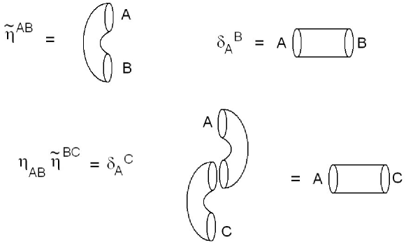
  Figure 2: The non-degeneracy equation and cobordisms.

  

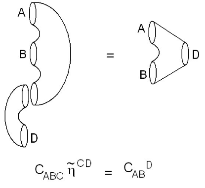
  Figure 3: Relating correlator to product

  

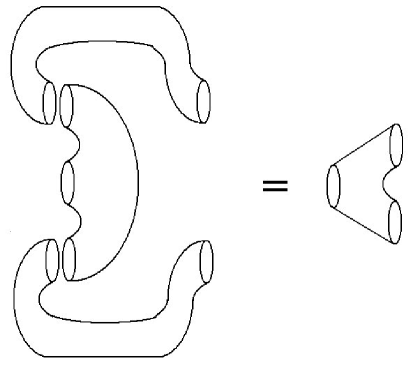
  Figure 4: Relating correlator to co-product

  

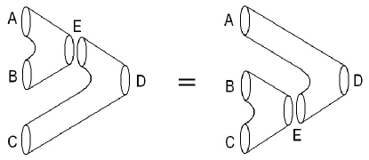
  Figure 5: Associativity and Crossing

• Higher point correlators can be constructed from three-point correlators, e.g

  $$C_{ABCD}=C_{AB}^{~{}~{}~{}E}C_{EC}^{~{}~{}~{}F}\eta_{FD}$$ (2.14)

  There is a similar construction for $n$-point correlators.

We will show that all these equations have realizations in the context of discrete data underlying correlators of CFT₄. These same equations are also realized by simpler toy-models. One of them is Gaussian integration. Another is related to $SU(2)$ fusions and has applications in the counting of primary fields. Both of these toy models have infinite dimensional state spaces. TFT₂ defined by these equations thus contains the discrete structure of CFT₄ as well as the related toy models. We will take these equations for $C_{ABC},\eta_{AB}$ as our definition of TFT₂ - they are essentially genus zero restrictions of standard TFT₂ equations. We have not given an axiomatic definition of the kind that exists for the case of usual TFT₂ (corresponding to Frobenius algebras) where all the possible gluings of the basic $\eta,C,\tilde{\eta}$ are allowed, higher genus surfaces are included and state spaces are constrained to be finite dimensional. Finding the right axiomatic framework for the equations presented here is an interesting problem, which we discuss in section 9.1.

2.3 Equations related to the properties of the vacuum state

As mentioned in the introduction and described in detail in section 4, the state space $\mathcal{W}$ in the case of the TFT₂ construction of CFT₄ is graded by the degree of the symmetric tensors

$$\mathcal{W}=\oplus_{n=0}\mathcal{W}_{n}\qquad\mathcal{W}_{n}=Sym(V^{\otimes n})$$ (2.15)

The pairing $\eta:\mathcal{W}\otimes\mathcal{W}\rightarrow{\bf{C}}$ is diagonal in the grading in the sense that

$$\eta(\mathcal{W}_{n},\mathcal{W}_{m})\propto\delta_{n,m}$$ (2.16)

The case $n=m=1$ is the case of the basic pairing, denoted $\hat{\eta}$. The case $n=m=2$ and higher corresponds to sums over all possible Wick contractions between composite fields, which are quadratic in $\varphi$ etc. The explicit formulae for $n\geq 1$ are in later sections. To describe the degree zero or vacuum sector introduce the state $e^{(0)}$ so that $\mathcal{W}_{0}=\mathbb{C}e^{(0)}$. That is, a general state in $\mathcal{W}_{0}$ is $ae^{(0)}$ for some complex number $a$. This is the one-dimensional representation of $SO(4,2)$. We define

$$\eta(e^{(0)},e^{(0)})=\eta_{00}=1$$ (2.17)

Then bilinearity requires that

$$\eta(a_{1}e^{(0)},a_{2}e^{(0)})=a_{1}a_{2}$$ (2.18)

Let us define the co-unit. This a homomorphism $\epsilon:\mathcal{W}\rightarrow\mathbb{C}$. It corresponds to the cobordism from circle to vacuum. We define

$$\epsilon(ae^{(0)}+e^{(1)}+e^{(2)}+\cdots)=a$$ (2.19)

It just picks up the coefficient of the vector in the trivial representation. Since this is a projector to the trivial irrep of $SO(4,2)$, it is $SO(4,2)$ equivariant. If we denote $e_{A}$ the general basis vectors of $\mathcal{W}$ (say a basis that diagonalizes the CFT inner product - which can be constructed by group theory) and we denote $A=0$ the vector $e^{(0)}$, then we have

$$\epsilon_{A}=\delta_{A,0}$$ (2.20)

Then we have the unit, which is a map $\tilde{\epsilon}:\mathbb{C}\rightarrow\mathcal{W}$. Pictorially it is the map from vacuum to circle.

$$\tilde{\epsilon}(1)=e^{(0)}$$ (2.21)

We define $\tilde{\epsilon}^{A}$ as the coefficient of the $A$’th basis vector in $\tilde{\epsilon}(1)$. Then we can write

$$\tilde{\epsilon}^{A}=\delta_{A,0}$$ (2.22)

And

$$\epsilon_{A}\tilde{\epsilon}^{A}=1$$ (2.23)

This means that the $S^{2}$ partition function of the TFT₂, which is obtained by gluing the vacuum-to-circle amplitude, with the circle-to-vacuum amplitude is $1$.

The definition of $C_{ABD}$ for general degree states is given later in terms of Wick-contractions. Letting $D$ be a degree zero state amounts to only having contractions between $A,B$. It follows that we will have

$$C_{AB0}=\eta_{AB}$$ (2.24)

When both $B,D$ are degree zero states,

$$C_{A00}\equiv\epsilon_{A}=\delta_{A0}$$ (2.25)

With these definitions, the equations corresponding to capping off an incoming circle or an outgoing circle hold.

If we have 3-circles going to vacuum, and cap off one circle, then we get just the amplitude for 2 circles going to vacuum.

$$C_{ABC}\tilde{\epsilon}^{C}=C_{ABC}\delta_{C,0}=C_{AB0}=\eta_{AB}$$ (2.26)

The figure for this equation is Figure 6.

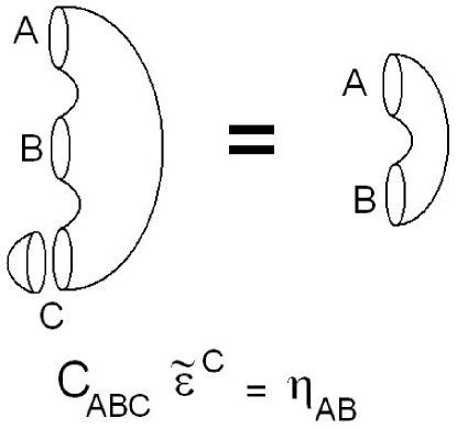
Figure 6: Capping 3-point correlator

For $\tilde{\eta}$, it makes sense to define

$$\tilde{\eta}^{A0}=\delta_{A0}$$ (2.27)

Then the equation

$$\eta_{AB}\tilde{\eta}^{BC}=\delta_{A}^{C}$$ (2.28)

becomes in the case $C=0$,

$$\eta_{AB}\tilde{\eta}^{B0}=\eta_{AB}\delta_{B,0}=\eta_{A,0}=\delta_{A,0}$$ (2.29)

which is consistent with the definition (2.27). We can write this as

$$\eta_{AB}\tilde{\eta}^{BC}\epsilon_{C}=\epsilon_{A}$$ (2.30)

The cobordism equivalence corresponding to this equation is Figure 7.

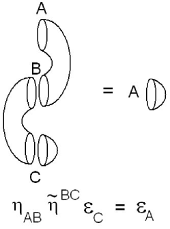
Figure 7: Capping the snake cylinder equation

2.4 Associativity and crossing equations

Here we use the non-degeneracy property (2.4) to show that associativity, crossing and Frobenius equations are equivalent. The Frobenius relation is given in Figure 8.

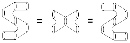
Figure 8: The Frobenius relation

The crossing equation is

$$C_{AB}^{~{}~{}~{}E}C_{CD}^{~{}~{}~{}F}\eta_{EF}=C_{BC}^{~{}~{}~{}E}C_{AD}^{~{}~{}~{}F}\eta_{EF}$$ (2.31)

Using the $\eta$ to lower indices

$$C_{CD}^{~{}~{}~{}F}\eta_{EF}=C_{CDE}=C_{ECD}=\eta_{EF}C^{F}_{~{}~{}CD}$$ (2.32)

The symmetry of $C$ follows because we have a CFT of bosons and is an algebraic property of the Wick contraction map acting on $\mathcal{W}\otimes\mathcal{W}\otimes\mathcal{W}$. We can do the same steps on the RHS and arrive at

$$C_{BC}^{~{}~{}~{}E}C_{EAD}$$ (2.33)

Now raise the $D$ index on both side using $\tilde{\eta}$ and we get the associativity equation is

$$C_{AB}^{~{}~{}~{}E}C_{EC}^{~{}~{}~{}D}=C_{BC}^{~{}~{}~{}E}C_{EA}^{~{}~{}~{}D}$$ (2.34)

We also have the Frobenius equation [1] ( sometimes called the nabla-delta equals delta-nabla relation), which can demonstrated using the existence of the inverse $\tilde{\eta}$ . Start from the nabla-delta equation

$$C_{AB}^{~{}~{}~{}E}C_{E}^{~{}~{}CD}=C_{A}^{~{}~{}ED}C_{EB}^{~{}~{}~{}C}$$ (2.35)

and lower the $C,D$ indices to obtain

$$C_{AB}^{~{}~{}~{}E}C_{ECD}=C_{AED}C^{E}_{~{}~{}~{}BC}$$ (2.36)

The RHS can be rearranged using the symmetry of $C_{...}$ as follows

$$C_{AED}C^{E}_{~{}~{}~{}BC}=C_{ADE}C^{E}_{~{}~{}~{}BC}=C_{AD}^{~{}~{}~{}E}C_{EBC}$$ (2.37)

This proves that the crossing equation implies both associativity and the equality of nabla-delta and delta-nabla. This last equation is called the Frobenius relation. These manipulations use the inverse of $\eta$, without ever encountering $\eta_{AB}\tilde{\eta}^{AB}$ which diverges.

2.5 Toy Model : Gaussian Integration

Our toy model employs the ring of polynomials in one variable. The states of the model are defined by

$$\phi_{n}=:x^{n}:=e^{-{1\over 2}\partial_{x}^{2}}x^{n}$$ (2.38)

It is straight forward to introduce an inner product on this space of states

$$g_{nm}=\langle\phi_{n}|\phi_{m}\rangle={\int dxe^{-x^{2}/2}:x^{n}:~{}:x^{m}:\over\int dxe^{-x^{2}/2}}$$ (2.39)

This inner product will play the role of the bilinear pairing of the TFT. Carrying out the integral above, we find

$$g_{nm}=\langle\phi_{n}|\phi_{m}\rangle=\delta_{nm}n!$$ (2.40)

Since $g_{nm}$ is clearly invertible, we have proved that this model has a non-degeneracy equation. Now, define the TFT structure constants by

$$C_{n_{1},n_{2},n_{3}}=\langle\phi_{n_{1}}\phi_{n_{2}}\phi_{n_{3}}\rangle$$ (2.41)

where

$$\langle\phi_{n_{1}}\phi_{n_{2}}\phi_{n_{3}}\cdots\phi_{n_{p}}\rangle={\int dxe^{-x^{2}/2}:x^{n_{1}}:~{}:x^{n_{2}}:~{}:x^{n_{3}}:~{}\cdots~{}:x^{n_{p}}:\over\int dxe^{-x^{2}/2}}$$ (2.42)

Again, carrying out the integral we find

$$C_{n_{1},n_{2},n_{3}}=\sum_{k=0}\delta(n_{3},n_{1}+n_{2}-2k)k!{n_{1}\choose k}{n_{2}\choose k}n_{3}!$$ (2.43)

The structure constants $C_{ab}^{~{}~{}c}$ give a product and we can get a co-product from $C_{a}^{~{}bc}$

$$\nabla(\phi_{a}\otimes\phi_{b})=C_{ab}^{~{}c}\phi_{c}$$ (2.44)

$$\Delta(\phi_{a})=C_{a}^{~{}bc}\phi_{b}\otimes\phi_{c}$$ (2.45)

The integral expression for $C_{abc}$ prove that the structure constants are symmetric. The above structure constants and bilinear pairing will define a TFT₂ provided the crossing equation

$$\langle\phi_{n_{1}}\phi_{n_{2}}\phi_{n_{3}}\phi_{n_{4}}\rangle=\sum_{m}C_{n_{1},n_{2},m}C_{n_{3},n_{4},m}{1\over m!}=\sum_{m}C_{n_{1},n_{3},m}C_{n_{4},n_{2},m}{1\over m!}$$ (2.46)

holds. Since the numerical values of the structure constants are given in (2.43), it is straightforward to verify (2.46) by plugging numbers in (e.g. with the help of Mathematica). More generally, it is clear that the crossing equation follows from the fact that the two expressions in (2.46) are two ways of calculating the integral (2.42). Thus, this model does indeed define a TFT.

A simple generalization of the above model, is to consider a Gaussian Hermitian matrix model. The natural analog of the observables above are parametrized by $[n,\sigma]$, where $n$ is a positive integer and $\sigma$ is a permutation in $S_{n}$

$$\phi_{[n,\sigma]} =:X^{i_{1}}_{i_{\sigma(1)}}\cdots X^{i_{n}}_{i_{\sigma(n)}}:$$ (2.49)

$$=e^{-{1\over 2}{\rm Tr}\left({d\over dX}{d\over dX}\right)}X^{i_{1}}_{i_{\sigma(1)}}\cdots X^{i_{n}}_{i_{\sigma(n)}}$$

$$\equiv e^{-{1\over 2}{\rm Tr}\left({d\over dX}{d\over dX}\right)}{\rm Tr}(\sigma X^{\otimes\,n})$$

Again, a natural inner product on this set of states ($dX$ is the usual $U(N)$ invariant measure for Hermitian matrices)

$$\langle\phi_{[n,\sigma]}|\phi_{[m,\tau]}\rangle={\int dX\,e^{-{1\over 2}{\rm Tr}(X^{2})}\,:{\rm Tr}(\sigma X^{\otimes\,n}):\,:{\rm Tr}(\tau X^{\otimes\,m}):\over\int dX\,e^{-{1\over 2}{\rm Tr}(X^{2})}}$$ (2.50)

gives us the bilinear pairing of the TFT. Carrying out the integral above, we find

$$\langle\phi_{[n,\sigma]}|\phi_{[m,\tau]}\rangle=\delta_{nm}\sum_{\sigma_{1}^{\prime}\in T_{1}}\sum_{\sigma_{2}^{\prime}\in T_{2}}\sum_{\sigma_{3}\in S_{n}}\delta(\sigma_{1}^{\prime}\sigma_{2}^{\prime}\sigma_{3})N^{C_{\sigma_{3}}}$$ (2.51)

$T_{1}$ is the conjugacy class of the permutation $\sigma$. $T_{2}$ is the conjugacy class of the permutation $\tau$. $C_{\sigma_{3}}$ is the number of cycles in the permutation $\sigma_{3}$. This model again has a non-degeneracy equation. Note however, the pairing (2.51) is not diagonal in this permutation basis. This will obscure the associativity of the model, although it could be verified by explicit computations. A simpler description is obtained by changing basis with a Fourier transform on the symmetric group

$$\phi_{[n,R]} ={1\over n!}\sum_{\sigma\in S_{n}}\chi_{R}(\sigma)\phi_{[n,\sigma]}$$ (2.53)

$$={1\over n!}\sum_{\sigma\in S_{n}}\chi_{R}(\sigma):X^{i_{1}}_{i_{\sigma(1)}}\cdots X^{i_{n}}_{i_{\sigma(n)}}:$$

Above $R\vdash n$ is a Young diagram with $n$ boxes and $\chi_{R}(\sigma)$ is a character of the symmetric group. Our states are now the Schur polynomials for which the pairing is diagonal

$$\langle\phi_{[n,R]}|\phi_{[m,S]}\rangle=\delta_{RS}f_{R}$$ (2.54)

with $f_{R}$ the product of the factors of Young diagram $R$ [4]. The TFT structure constants are now

$$C_{[n,R],[m,S],[p,T]}=\langle\phi_{[n,R]}\phi_{[m,S]}\phi_{[p,T]}\rangle$$ (2.55)

where

$$\langle\phi_{[n_{1},R_{1}]}\cdots\phi_{[n_{p},R_{p}]}\rangle={\int dM\,e^{-{1\over 2}{\rm Tr}(M^{2})}\,\phi_{[n_{1},R_{1}]}\,\cdots\,\phi_{[n_{p},R_{p}]}\over\int dM\,e^{-{1\over 2}{\rm Tr}(M^{2})}}$$

The crossing equation

$$\langle\phi_{[n_{1},R_{1}]}\phi_{[n_{2},R_{2}]}\phi_{[n_{3},R_{3}]}\phi_{[n_{4},R_{4}]}\rangle =\sum_{p=|n_{1}-n_{2}|}^{n_{1}+n_{2}}\sum_{R}C_{[n_{1},R_{1}],[n_{2},R_{2}],[p,R]}C_{[n_{3},R_{3}],[n_{4},R_{4}],[p,R]}{1\over f_{R}}$$ (2.58)

$$=\sum_{p=|n_{1}-n_{3}|}^{n_{1}+n_{3}}\sum_{R}C_{[n_{1},R_{1}],[n_{3},R_{3}],[p,R]}C_{[n_{4},R_{4}],[n_{2},R_{2}],[p,R]}{1\over f_{R}}$$

will hold because, again, the two expressions appearing above are two ways of calculating the integral needed to evaluate the right hand side. The product takes the form

$$\phi_{[n_{1},R_{1}]}*\phi_{[n_{2},R_{2}]}=\sum_{k}C(n_{1},n_{2},k,R_{1},R_{2},R_{1}*_{k}R_{2})\phi_{[n_{1}+n_{2}-2k,R_{1}*_{k}R_{2}]}$$ (2.59)

where $C(n_{1},n_{2},k,R_{1},R_{2},R_{1}*_{k}R_{2})\in\mathbb{Z}$ is a combinatoric factor. We have defined a star-product labeled by $k$. In this Fourier basis of Young diagrams, the $k=0$ product is given by Littlewood-Richardson coefficients. In the original permutation basis this is the outer product which takes $\sigma_{1}\in S_{n_{1}},\sigma_{2}\in S_{n_{2}}$ to give $(\sigma_{1}\circ\sigma_{2})\in S_{n_{1}}\times S_{n_{2}}\in S_{n_{1}+n_{2}}$. For the case, $n_{1}=n_{2}$ and $k=n_{1}=n_{2}$, the product is the ordinary product of permutations. The intermediate cases correspond to products where one permutation acts on a set of $n_{1}$ integers, the second on a subset of $n_{2}$ integers, where the sets overlap over $k$ elements. This structure is readily derived using diagrammatic tensor space techniques [20, 21].

2.6 Zero area YM2 : An example of infinite dimensional state spaces and restricted amplitudes

In the above discussions and in most of the paper, we focus on examples where TFT₂ with infinite dimensional state spaces arise, with a restriction to genus zero. There are also examples where infinite dimensional state spaces arise, and infinities are avoided by restricting to surfaces of genus greater than one. The partition function of YM2 on a surface of genus $G$ with area $A$ [22], with $g_{YM}^{2}$ set to $1$, is

$$Z_{YM2}(G,A)=\sum_{R}(DimR)^{2-2G}e^{-AC_{2}(R)}$$ (2.60)

where the sum is over irreps $R$ of the gauge group, $DimR$ is the dimension of the representation $R$, $C_{2}(R)$ is the quadratic Casimir. In the zero area limit, we have

$$Z_{YM2}(G,A=0)=\sum_{R}(DimR)^{2-2G}$$ (2.61)

This diverges for $G=0,1$ for a Lie group, e.g. $SU(N)$, since there are infinitely many irreps with arbitrarily large dimensions. However the partition function is well defined for $G>1$. The $A=0$ limit is interesting as a topological limit, from the point of view of the moduli space of flat $SU(N)$ connections [23] and also from the large $N$ expansion and gauge-string duality [24, 25].

3 Basic CFT₄ 2-point function as an invariant map in TFT₂

In free massless scalar field theory in four dimensions, all the correlators of composite local operators inserted at distinct points, can be obtained from the basic 2-point function of the elementary field

$$\langle\varphi(x_{1})\varphi(x_{2})\rangle={1\over(x_{1}-x_{2})^{2}}\equiv G(x_{1},x_{2})$$ (3.1)

where $x_{1}^{\mu},x_{2}^{\mu}$ are points in $\mathbb{R}^{4}$. If we transform $\varphi(x_{2})\rightarrow\varphi^{\prime}(x_{2}^{\prime})$ where $x_{2}^{\prime}={x_{2}\over x_{2}^{2}}$ , we encounter

$$\langle\varphi(x_{1})\varphi^{\prime}(x_{2}^{\prime})\rangle=(x_{2})^{2}\langle\varphi(x_{1})\varphi(x_{2})\rangle={1\over(1-2x_{1}\cdot x_{2}^{\prime}+(x_{2}^{\prime})^{2}x_{1}^{2})}\equiv F(x_{1},x_{2}^{\prime})$$ (3.2)

In this section we will show that this quantity encodes the way the one-dimensional representation $\mathbb{C}$ appears inside the tensor product $V_{+}\otimes V_{-}$. The representation $V_{+}$ is the irrep of $SO(4,2)$ where the lowest energy state has dimension $D=1$, corresponding to the state $\varphi$ of CFT₄, and the other states correspond to derivatives of $\varphi$, or equivalently to strings of $P_{\mu}$ acting on the lowest weight state. We use energy/dimension/weight interchangeably in this paper, since we are working with radial quantization. Its conjugate is $V_{-}$ which is the representation with highest weight (energy) having $D=-1$ and where states are generated by $K_{\mu}$.

We start by describing the properties of the bilinear $SO(4,2)$ invariant map $\hat{\eta}:V_{+}\otimes V_{-}\rightarrow\mathbb{C}$. A Lie algebra element $\mathcal{L}\in so(4,2)$ acts on the tensor product as

$$\mathcal{L}\otimes 1+1\otimes\mathcal{L}\equiv\Delta(\mathcal{L})$$ (3.3)

The complex number field is the one-dimensional representation where the Lie algebra acts as zero. An equivariant map $\hat{\eta}$ to $\mathbb{C}$ obeys

$$\Delta(\mathcal{L})\circ\hat{\eta}=\hat{\eta}\circ\Delta(\mathcal{L})$$ (3.4)

The LHS is zero because $\mathbb{C}$ is the trivial irrep, and the expanding the RHS gives

$$\hat{\eta}(\mathcal{L}v_{1},v_{2})+\hat{\eta}(v_{1},\mathcal{L}v_{2})=0$$ (3.5)

This equivariance property exactly fits the definition of what is required in TFT₂ with $SO(4,2)$ as global symmetry.

The requirement that this map is $SO(4,2)$ invariant fixes it up to an overall constant. Equivalently the decomposition of the tensor product $V_{+}\otimes V_{-}$ in terms of irreducible representations contains a unique copy of the trivial one-dimensional representation $\mathbb{C}$, where the Lie algebra elements act as zero. The states in $V_{+}$ are of the form

$$C^{I}_{\mu_{1}\cdots\mu_{n}}P_{\mu_{1}}\cdots P_{\mu_{n}}v^{+}$$ (3.6)

where the $C^{I}$ are symmetric traceless tensors. We will introduce (Euclidean) spacetime coordinates $x^{\mu}$ to keep track of these states. We can think of $x^{\mu}$ as a way to describe the states in $V_{+}$ via a continuous variable as opposed to a discrete variable. Analogously for $V_{-}$ we have states obtained by acting with $K_{\mu}$ and the variable $x^{\prime}$ is the continuous variable. We will show that the invariant map $\hat{\eta}$, described in this spacetime basis is the 2-point function $F(x_{1},x_{2}^{\prime})$. Further, in the spacetime basis, there are a simple set of differential equations expressing the $SO(4,2)$ invariance of $\hat{\eta}$. Finally, using $\hat{\eta}$ and a map $\rho:V_{+}\to V_{-}$ we are able to define an inner product on $V_{+}$ and on $V_{-}$. This is a map from $V_{\pm}\times V_{\pm}$ to $\mathbb{C}$ which is sesquilinear. The inner product obtained in this way is the usual one which is used, for example, to study the bounds unitarity places on operator dimensions[26].

3.1 Flat space quantization and radial quantization

Start from the $so(4,2)$ algebra (we use $g={\rm diag}(-,-,+,...,+)\,\,\,)$

$$\left[S_{MN},S_{PQ}\right]=g_{NP}S_{MQ}+g_{MQ}S_{NP}-g_{MP}S_{NQ}-g_{NQ}S_{MP}$$ (3.7)

The indices $M,N,\cdots$ run over $\{-1,0,1,\cdots d\}$. Note that the structure constants are all real and the generators are all antihermittian $S_{MN}^{\dagger}=-S_{MN}$. We can write this algebra in two different ways, which make different subgroups manifest. For useful background material see [27] and section 2.1.2 of [28].

3.1.1 Manifest $so(3,1)\times so(1,1)$ subgroup

This rewriting is relevant for quantization of the theory on $R^{4}$ or $R^{3,1}$. Each equal time slice is a copy of 3-dimensional Euclidean space, $R^{3}$. Identify

$$M_{\mu\nu}^{\prime} = S_{\mu\nu}\qquad D^{\prime}=S_{-1,d}$$ (3.8)

$$P_{\mu}^{\prime} = S_{\mu,-1}+S_{\mu,d}\qquad K^{\prime}_{\mu}=S_{\mu,-1}-S_{\mu,d}$$ (3.9)

with $\mu\in\{0,1,\cdots,d-1\}$. From the anti-hermiticity of the $S_{MN}$s we find

$$(M_{\mu\nu}^{\prime})^{\dagger} = -M_{\mu\nu}^{\prime}\qquad(D^{\prime})^{\dagger}=-D^{\prime}$$ (3.10)

$$(P^{\prime}_{\mu})^{\dagger} = -P^{\prime}_{\mu}\qquad(K^{\prime}_{\mu})^{\dagger}=-K^{\prime}_{\mu}$$ (3.11)

i.e. all of the generators have pure imaginary eigenvalues. The algebra obeyed by these generators is

$$\big{[}M_{\mu\nu}^{\prime},M^{\prime}_{\alpha\beta}\big{]} = g_{\mu\beta}M^{\prime}_{\nu\alpha}+g_{\nu\alpha}M^{\prime}_{\mu\beta}-g_{\mu\alpha}M^{\prime}_{\nu\beta}-g_{\nu\beta}M^{\prime}_{\mu\alpha}$$ (3.12)

$$\big{[}M_{\mu\nu}^{\prime},D^{\prime}\big{]} = 0\qquad\big{[}D^{\prime},P^{\prime}_{\rho}\big{]}=-P^{\prime}_{\rho}\qquad\big{[}D^{\prime},K^{\prime}_{\rho}\big{]}=K^{\prime}_{\rho}$$ (3.13)

$$\big{[}M_{\mu\nu}^{\prime},P^{\prime}_{\rho}\big{]} = g_{\nu\rho}P^{\prime}_{\mu}-g_{\mu\rho}P^{\prime}_{\nu}\qquad\big{[}M_{\mu\nu}^{\prime},K^{\prime}_{\rho}\big{]}=g_{\nu\rho}K^{\prime}_{\mu}-g_{\mu\rho}K^{\prime}_{\nu}$$ (3.14)

$$\big{[}K_{\mu}^{\prime},P_{\nu}^{\prime}\big{]} = 2M^{\prime}_{\mu\nu}-2g_{\mu\nu}D^{\prime}$$ (3.15)

Notice that the $M_{\mu\nu}^{\prime}$ generate $SO(3,1)$ and $D^{\prime}$ generates $SO(1,1)$.

3.1.2 Manifest $so(4)\times so(2)$ subgroup

This rewriting is relevant for the radial quantization. Equal “time slices” are three-spheres, $S^{3}$. Identify

$$M_{pq} = S_{pq}\qquad D=iS_{-1,0}$$ (3.16)

$$P_{p} = S_{p,-1}+iS_{p,0}\qquad K_{p}=S_{p,-1}-iS_{p,0}$$ (3.17)

with $p\in\{1,\cdots,d\}$. Notice that from the anti-hermitticity of the $S_{MN}$’s we find

$$(M_{pq})^{\dagger} = -M_{pq},\qquad(D)^{\dagger}=D$$ (3.18)

$$(P_{p})^{\dagger} = -K_{p},\qquad(K_{p})^{\dagger}=-P_{p}$$ (3.19)

Thus, $D$ will have real eigenvalues and $M_{pq}$ will have purely imaginary eigenvalues. The algebra obeyed by these generators is

$$\big{[}M_{pq},M_{rs}\big{]} = \delta_{qr}M_{ps}+\delta_{ps}M_{qr}-\delta_{qs}M_{pr}-\delta_{pr}M_{qs}$$ (3.20)

$$\big{[}M_{pq},D\big{]} = 0\qquad\big{[}D,P_{p}\big{]}=P_{p}\qquad\big{[}D,K_{p}\big{]}=-K_{p}$$ (3.21)

$$\big{[}M_{pq},P_{r}\big{]} = \delta_{qr}P_{p}-\delta_{pr}P_{q}\qquad\big{[}M_{pq},K_{r}\big{]}=\delta_{qr}K_{p}-\delta_{pr}K_{q}$$ (3.22)

$$\big{[}K_{p},P_{q}\big{]} = 2M_{pq}-2\delta_{pq}D$$ (3.23)

Clearly then, $M_{pq}$ generate the $SO(4)$ subgroup, while $D$ generates the $SO(2)$ subgroup.

3.2 Invariant pairing

We will use the writing of $so(4,2)$ which makes the $so(4)\times so(2)$ subalgebra manifest. We want to consider two different $so(4,2)$ representations $V_{+}$ and $V_{-}$. $V_{+}$ is built on the lowest weight state $v^{+}$ which obeys

$$Dv^{+}=dv^{+}\qquad M_{pq}v^{+}=0$$ (3.24)

The remaining states in this irrep are constructed by acting with traceless combinations of $P_{p}$s on $v^{+}$. A convenient way to describe this is to write

$$v^{+,I,l}=C^{I}_{p_{1}\cdots p_{l}}P_{p_{1}}\cdots P_{p_{l}}v^{+}$$ (3.25)

where the tensor $C^{I}_{p_{1}\cdots p_{l}}$ is symmetric traceless in the $p_{1},\cdots,p_{l}$ indices. The index $I$ runs over the states in the $SO(4)$ irrep $({l\over 2},{l\over 2})$. We will often trade $I$ for $SU(2)\times SU(2)$ state labels $(m_{L},m_{R})$.

$V^{-}$ is built on the highest weight state $v^{-}$ which obeys

$$Dv^{-}=-dv^{-}\qquad M_{pq}v^{-}=0$$ (3.26)

The remaining states in this irrep are constructed by acting with traceless combinations of $K_{p}$’s on $v^{-}$. The representations that we consider most of the time are relevant for the description of a free massless bosonic scalar field in 4 dimensions, in which case we set $d=1$. For the remainder of this section, we will set $d=1$.

The invariant pairing is $\hat{\eta}:V_{+}\otimes V_{-}\rightarrow\mathbb{C}$. Concretely

$$\hat{\eta}\left(C^{I}_{p_{1}\cdots p_{l}}P_{p_{1}}\cdots P_{p_{l}}v^{+},C^{J}_{q_{1}\cdots q_{l^{\prime}}}K_{q_{1}}\cdots K_{q_{l^{\prime}}}v^{-}\right)=f_{l,m_{L},m_{R};l^{\prime}m_{L}^{\prime},m_{R}^{\prime}}$$ (3.27)

On the right hand side we have traded $I$ for $(m_{L},m_{R})$ and $J$ for $(m_{L}^{\prime},m_{R}^{\prime})$. In the next section we will prove that the requirement of $so(4,2)$ invariance determines $f_{l,m_{L},m_{R};l^{\prime}m_{L}^{\prime},m_{R}^{\prime}}$ up to an overall constant. A convenient way of summarizing the action of $\hat{\eta}$ is in terms of the tensors

$$T_{p_{1}p_{2}\cdots p_{n},q_{1}q_{2}\cdots q_{n}}=\hat{\eta}\left(P_{p_{1}}P_{p_{2}}\cdots P_{p_{n}}v^{+},K_{q_{1}}K_{q_{2}}\cdots K_{q_{n}}v^{-}\right)$$ (3.28)

which are themselves nicely summarized as

$$T_{p_{1}\cdots p_{n},q_{1}\cdots q_{n}}\prod_{a=1}^{n}y^{\prime q_{a}}x^{p_{a}}=2^{n}n!\sum_{l=0}^{\big{[}{n\over 2}\big{]}}(-1)^{l}(x\cdot y^{\prime})^{n-2l}|x|^{2l}|y^{\prime}|^{2l}{(n-l)!n!\over(n-2l)!2^{2l}l!}$$ (3.29)

To evaluate (3.28), we can use the $so(4,2)$ invariance of the pairing to shift (say) $P_{p}$’s from the left slot to the right slot. The action of $P_{p}$ on the state in the right slot is then easily computed by using the $so(4,2)$ algebra as well as the fact that $P_{p}$ annihilates $v^{-}$. In the next section, this logic will be applied also to $SU(2)\times SU(2)$ and $SL(2)$ sub-algebras, to derive an explicit formula for $f_{l,m_{L},m_{R};l^{\prime}m_{L}^{\prime},m_{R}^{\prime}}$. A straight forward computation now gives

$$F(x,y^{\prime}) \equiv\hat{\eta}\left(e^{-ix\cdot P^{\prime}}v^{+},e^{iy^{\prime}\cdot K^{\prime}}v^{-}\right)$$ (3.33)

$$=\sum_{n=0}^{\infty}T_{p_{1}\cdots p_{n},q_{1}\cdots q_{n}}\prod_{a=1}^{n}y^{\prime q_{a}}x^{p_{a}}{1\over(n!)^{2}}$$

$$=\sum_{n=0}^{\infty}2^{n}\sum_{l=0}^{\big{[}{n\over 2}\big{]}}(-1)^{l}(x\cdot y^{\prime})^{n-2l}|x|^{2l}|y^{\prime}|^{2l}{(n-l)!\over(n-2l)!2^{2l}l!}$$

$$={1\over 1-2x\cdot y^{\prime}+x^{2}y^{\prime 2}}$$

For a closely related discussion, see section 3 of [29].

3.2.1 Description of pairing in terms of $SU(2)\times SU(2)$ and $SL(2)$ subalgebras

The requirement of $so(4,2)$ invariance determines $f_{l,m_{L},m_{R};l^{\prime}m_{L}^{\prime},m_{R}^{\prime}}$ up to an overall constant. This is most easily demonstrated by requiring that $\hat{\eta}$ is invariant under $sl(2)$ and $su(2)\times su(2)$ subalgebras. We will prove that the $\hat{\eta}$ obtained in this way enjoys the full $so(4,2)$ invariance.

The complete set of states of $V_{+}$ can be obtained by acting with elements of the $sl(2)$ and $su(2)\times su(2)$ subalgebras on $v^{+}$, and the complete set of states of $V_{-}$ can be obtained by acting with elements of the $sl(2)$ and $su(2)\times su(2)$ algebras on $v^{-}$. This can be seen by considering the $SO(4,2)$ character in equation (B.7) for $V_{+}$. The coefficient of $s^{q+1}$ in this character

$$\chi_{V_{+}}(s,x,y)=\sum_{q=0}^{\infty}s^{q+1}\chi_{q\over 2}(x)\chi_{q\over 2}(y)$$ (3.34)

is $\chi_{q\over 2}(x)\chi_{q\over 2}(y)$. This implies that the states of scaling dimension $q+1$ fill out a multiplet of spin $(j_{L},j_{R})=({q\over 2},{q\over 2})$. This complete multiplet can be generated by applying $SU(2)\times SU(2)$ rotations to $(H_{+})^{q}v^{+}$, which shows that we do indeed generate the complete set of states in $V_{+}$ by acting with the $sl(2)$ and $su(2)\times su(2)$ subalgebras on $v^{+}$. A similar argument shows that we generate the complete set of states of dimension $-q-1$ in $V_{-}$ by acting with elements of $su(2)\times su(2)$ on $(H_{-})^{q}v^{-}$.

Invariance under $sl(2)$ and $su(2)\times su(2)$ leads to

$$f_{l,m_{L},m_{R};l^{\prime},m_{L}^{\prime},m_{R}^{\prime}}=f_{l}\left(SL(2)\right)f_{m_{L}}\left(SU(2)\right)f_{m_{R}}\left(SU(2)\right)\delta_{l,l^{\prime}}\delta_{m_{L},-m_{L}^{\prime}}\delta_{m_{R},-m_{R}^{\prime}}$$ (3.35)

We will demonstrate how invariance under $sl(2)$ fixes $f_{l}\left(SL(2)\right)$. The demonstrations for $f_{m_{L}}\left(SU(2)\right)$ and $f_{m_{R}}\left(SU(2)\right)$ are very similar.

The subalgebra that we study is described in detail in Appendix A. The two $su(2)$ algebras have raising and lowering operators given by $J_{\pm}^{R}$ and $J_{\pm}^{L}$, while the raising and lowering operators of $sl(2)$ are $H_{\pm}$. In terms of these generators, the pairing $\hat{\eta}$ is

$$\hat{\eta}((J_{+}^{R})^{p_{R}}(J_{+}^{L})^{p_{L}}(H_{+})^{l}v^{+},(J_{-}^{R})^{p_{R}^{\prime}}(J_{-}^{L})^{p_{L}^{\prime}}(H_{-})^{l^{\prime}}v^{-})=\delta_{p_{L},p_{L}^{\prime}}\delta_{p_{R},p_{R}^{\prime}}\delta_{l,l^{\prime}}f_{l,p_{L}}^{su(2)}f_{l,p_{R}}^{su(2)}f_{d,l}^{sl(2)}$$ (3.36)

To demonstrate how $sl(2)$ invariance fixes $f_{d,l}^{sl(2)}$, consider the positive discrete series irrep $\tilde{V}_{+}$ of $sl(2)$ and the negative discrete series irrep $\tilde{V}_{-}$

$$\tilde{V}_{+}=Span\{H_{+}^{l}v^{+}~{}~{}:~{}~{}H_{-}v^{+}=0~{}~{},~{}~{}H_{3}v^{+}=dv^{+}\}$$ (3.37)

$$\tilde{V}_{-}=Span\{H_{-}^{l}v^{-}~{}~{}:~{}~{}H_{+}v^{-}=0~{}~{},~{}~{}H_{3}v^{-}=-dv^{-}\}$$ (3.38)

Note that $\tilde{V}_{\pm}$ are subspaces of the irreducible $SO(4,2)$ representations $V_{\pm}$ that we introduced above. Invariance of the pairing $\hat{\eta}(H_{+}^{l}v^{+},H_{-}^{l^{\prime}}v^{-})$ under $H_{3}$ gives

$$\Delta(H_{3})\,\,\hat{\eta}(H_{+}^{l}v^{+},H_{-}^{l^{\prime}}v^{-}) = \hat{\eta}(H_{3}H_{+}^{l}v^{+},H_{-}^{l^{\prime}}v^{-})+\hat{\eta}(H_{+}^{l}v^{+},H_{3}H_{-}^{l^{\prime}}v^{-})$$ (3.39)

$$= ((d+l)-(d+l^{\prime}))\hat{\eta}(H_{+}^{l}v^{+},H_{-}^{l^{\prime}}v^{-})$$ (3.40)

which shows it vanishes unless $l=l^{\prime}$, so that

$$\hat{\eta}(H_{+}^{l}v^{+},H_{-}^{l^{\prime}}v^{-})=f_{d,l}^{sl(2)}\delta_{ll^{\prime}}$$ (3.41)

Then we have

$$\Delta(H_{-})\,\,\hat{\eta}(H_{+}^{l}v^{+},H_{-}^{l^{\prime}}v^{-}) = \hat{\eta}(H_{-}H_{+}^{l}v^{+},H_{-}^{l^{\prime}}v^{-})+\hat{\eta}(H_{+}^{l}v^{+},H_{-}^{l^{\prime}+1}v^{-})$$ (3.42)

$$= \delta_{l,l^{\prime}+1}(\sum_{i=0}^{l-1}(-2i+d)f_{d,l-1}^{sl(2)}+f_{d,l}^{sl(2)})$$ (3.43)

which gives

$$f_{l,d}^{sl(2)}=l(l+d-1)f_{l-1,d}^{sl(2)}$$ (3.44)

This is solved by

$$f_{l,d}^{sl(2)}=l!{(d+l-1)!\over(d-1)!}$$ (3.45)

A very similar argument requiring invariance under $su(2)$, shows that

$$f^{su(2)}_{l,p}=(-1)^{p}{l!p!\over(l-p)!}$$ (3.46)

3.2.2 $so(4,2)$ invariance of the pairing

To obtain the pairing $\hat{\eta}$ we have required invariance under the $sl(2)$ and $su(2)\times su(2)$ algebras. In this section we will show that the pairing we have obtained enjoys the bigger $so(4,2)$ invariance. The requirement of $so(4,2)$ invariance translates into a set of partial differential equations for $F(x,y^{\prime})$. The demonstration then amounts to showing the $F(x,y^{\prime})$ does indeed obey these partial differential equations.

Recall that

$$F(x,y^{\prime})=\hat{\eta}\left(e^{-ix\cdot P}v^{+},e^{iy^{\prime}\cdot K}v^{-}\right)$$ (3.47)

To start, we will consider invariance under dilatations. Towards this end, note that

$$De^{-ix\cdot P}v^{+}=\sum_{n=0}^{\infty}(n+1){(-ix\cdot P)^{n}\over n!}v^{+}=\left(x\cdot{\partial\over\partial x}+1\right)e^{-ix\cdot P}v^{+}$$ (3.48)

and

$$De^{iy^{\prime}\cdot K}v^{-}=-\sum_{n=0}^{\infty}(n+1){(iy^{\prime}\cdot K)^{n}\over n!}v^{-}=-\left(y^{\prime}\cdot{\partial\over\partial y^{\prime}}+1\right)e^{iy^{\prime}\cdot K}v^{-}$$ (3.49)

Thus, the statement of invariance under dilatations

$$\Delta(D)\,\,\hat{\eta}\left(e^{-ix\cdot P}v^{+},e^{iy^{\prime}\cdot K}v^{-}\right)=0$$ (3.50)

is equivalent to the differential equation

$$\left(x\cdot{\partial\over\partial x}-y^{\prime}\cdot{\partial\over\partial y^{\prime}}\right)F(x,y^{\prime})=0$$ (3.51)

It is straightforward to check that the function given in (3.33) obeys this equation.

Next, some algebra shows that

$$P_{p}(y^{\prime}\cdot K)^{n}v^{-}= n(n-1)[(y^{\prime}\cdot K)y_{p}^{\prime}-(y^{\prime})^{2}K_{p}](-iy^{\prime}\cdot K)^{n-2}v^{-}$$ (3.53)

$$+iy_{p}^{\prime}n(n+1)(-iy^{\prime}\cdot K)^{n-1}v^{-}$$

which implies

$$P_{p}e^{iy^{\prime}\cdot K}v^{-}=-\big{[}2iy_{p}^{\prime}y^{\prime}\cdot{\partial\over\partial y^{\prime}}-i(y^{\prime})^{2}{\partial\over\partial y_{p}^{\prime}}+2iy_{p}^{\prime}\big{]}e^{iy^{\prime}\cdot K}v^{-}$$ (3.54)

It is also clear that

$$P_{p}e^{-ix\cdot P}v^{+}=i{\partial\over\partial x^{p}}e^{-ix\cdot P}v^{+}$$ (3.55)

Consequently, the statement

$$\Delta(P_{p})\,\,\hat{\eta}\left(e^{-ix\cdot P}v^{+},e^{iy^{\prime}\cdot K}v^{-}\right)=0$$ (3.56)

is equivalent to the differential equation

$$\left[i{\partial\over\partial x^{p}}-2iy_{p}^{\prime}y^{\prime}\cdot{\partial\over\partial y^{\prime}}+i(y^{\prime})^{2}{\partial\over\partial y_{p}^{\prime}}-2iy_{p}^{\prime}\right]F(x,y^{\prime})=0$$ (3.57)

Again, this equation is obeyed by (3.33).

Finally, note that

$$M_{pq}(iy^{\prime}\cdot K)^{n}v^{-}=in(y_{p}^{\prime}K_{q}-y_{q}^{\prime}K_{p})(iy^{\prime}\cdot K)^{n-1}v^{-}$$ (3.58)

and

$$M_{pq}(-ix\cdot P)^{n}v^{+}=-in(x_{p}P_{q}-x_{q}P_{p})(-ix\cdot P)^{n-1}v^{+}$$ (3.59)

Consequently, the statement

$$\Delta(M_{pq})\,\,\hat{\eta}\left(e^{-ix\cdot P}v^{+},e^{iy^{\prime}\cdot K}v^{-}\right)=0$$ (3.60)

is equivalent to the differential equation

$$\left[x_{p}{\partial\over\partial x_{q}}-x_{q}{\partial\over\partial x_{p}}+y^{\prime}_{p}{\partial\over\partial y^{\prime}_{q}}-y^{\prime}_{q}{\partial\over\partial y^{\prime}_{p}}\right]F(x,y^{\prime})=0$$ (3.61)

This equation is again obeyed by (3.33), which completes the demonstration of $so(4,2)$ invariance.

3.3 Invariant pairing to Inner product via twist map $\rho$

In this section we define an inner product $g:V_{\pm}\times V_{\pm}\to\mathbb{C}$. Since we have the invariant map $\hat{\eta}:V_{+}\times V_{-}\to\mathbb{C}$, if we introduce a map $\rho:V_{+}\rightarrow V_{-}$ we can construct an inner product by composing $\rho$ and $\hat{\eta}$. We will choose the map $\rho$ so that the inner product obtained is the usual inner product of the CFT used to test unitarity. The positivity of this inner product is what puts constraints on dimensions of fields. For example, a scalar should not have dimension lower than $1$, as first proved by Mack [26]. $\hat{\eta}$ is the building block of $SO(4,2)$ invariant maps, which can be used to construct correlators. The $\rho$ map gives the relation between $\hat{\eta}$ and $g$, and is related to an automorphism.

The map $\rho:V_{+}\rightarrow V_{-}$ is given by

$$\rho(P_{\mu_{1}}P_{\mu_{2}}\cdots P_{\mu_{n}}v^{+})=K_{\mu_{1}}\cdots K_{\mu_{n}}v^{-}$$ (3.62)

This map obeys the conditions

$$\rho(\mathcal{L}_{a}v_{1})=-\mathcal{L}_{a}^{\dagger}\rho(v_{1})$$ (3.63)

for any $v_{1}$. The dagger of the generators is given in (3.19). We also define

$$\rho(\lambda v_{1})=\lambda^{*}\rho(v_{1})$$ (3.64)

for complex scalars $\lambda$. The inner product is now given by

$$g(v_{1},v_{2})=\hat{\eta}(\rho(v_{1}),v_{2})$$ (3.65)

This construction of a sesquilinear inner product from a bilinear pairing appears in the context of 3-dimensional TFT in [30]. Consistency is guaranteed by checking that $g(v_{1},v_{2})$ has the properties of the inner product

$$g(v_{1},v_{2})=(g(v_{2},v_{1}))^{*}$$ (3.66)

$$g(v_{1},\lambda v_{2})=\lambda g(v_{1},v_{2})$$ (3.67)

$$g(\lambda v_{1},v_{2})=\lambda^{*}g(v_{1},v_{2})$$ (3.68)

To see the last two of these,

$$g(v_{1},\lambda v_{2})=\hat{\eta}(\rho(v_{1}),\lambda v_{2})=\lambda\hat{\eta}(\rho(v_{1}),v_{2})=\lambda g(v_{1},v_{2})$$ (3.69)

$$g(\lambda v_{1},v_{2})=\hat{\eta}(\rho(\lambda v_{1}),v_{2})=\hat{\eta}(\lambda^{*}\rho(v_{1}),v_{2})=\lambda^{*}g(v_{1},v_{2})$$ (3.70)

We have used the bilinearity of $\hat{\eta}$ and the definition $\rho(\lambda v)=\lambda^{*}\rho(v)$. To see the symmetry consider

$$g(\lambda_{1}P_{\mu_{1}}\cdots P_{\mu_{n}}v^{+},\lambda_{2}P_{\nu_{1}}\cdots P_{\nu_{n}}v^{+})$$ (3.71)

$$=\lambda_{1}^{*}\lambda_{2}\hat{\eta}(K_{\mu_{1}}\cdots K_{\mu_{n}}v^{-},P_{\nu_{1}}\cdots P_{\nu_{n}}v^{+})$$ (3.72)

$$=\lambda_{1}^{*}\lambda_{2}T_{\vec{\mu},\vec{\nu}}$$ (3.73)

and

$$g(\lambda_{2}P_{\nu_{1}}\cdots P_{\nu_{n}}v^{+},\lambda_{1}P_{\mu_{1}}\cdots P_{\mu_{n}}v^{+})$$ (3.74)

$$=\lambda_{2}^{*}\lambda_{1}\hat{\eta}(K_{\nu_{1}}\cdots K_{\nu_{n}}v^{-},P_{\mu_{1}}\cdots P_{\mu_{n}}v^{+}$$ (3.75)

$$=\lambda_{2}^{*}\lambda_{1}T_{\vec{\nu},\vec{\mu}}$$ (3.76)

The explicit formulae (3.29) show that $T_{\vec{\mu},\vec{\nu}}=T_{\vec{\nu},\vec{\mu}}$ and $T_{\vec{\mu},\vec{\nu}}^{*}=T_{\vec{\mu},\vec{\nu}}$. This proves $g(v_{1},v_{2})=(g(v_{2},v_{1}))^{*}$.

It is also useful to note that

$$g(\mathcal{L}_{a}v_{1},v_{2})=\eta(\rho(\mathcal{L}_{a}v_{1}),v_{2})=-\eta(\mathcal{L}_{a}^{\dagger}\rho(v_{1}),v_{2})=\eta(\rho(v_{1}),\mathcal{L}_{a}^{\dagger}v_{2})=g(v_{1},\mathcal{L}_{a}^{\dagger}v_{2})$$ (3.77)

This explains why this inner product has the usual hermiticity property. Finally we observe that the map $\alpha(\mathcal{L}_{a})\equiv-\mathcal{L}_{a}^{\dagger}$ used above is an automorphism of the Lie algebra

$$[\alpha(\mathcal{L}_{a}),\alpha(\mathcal{L}_{b})]=\alpha([\mathcal{L}_{a},\mathcal{L}_{b}])$$ (3.78)

4 State space, amplitudes, and correlators in the TFT₂

In section 3 we have made use of two representations $V_{+}$ and $V_{-}$. This has allowed us to describe the two point function of the basic field of free scalar field theory in four dimensions in terms of the invariant irrep $\mathbb{C}$ of $SO(4,2)$ appearing in the tensor product $V_{+}\otimes V_{-}$. In this section we will consider a larger state space $\mathcal{W}$, which will allow us to extend our discussion to arbitrary correlation functions in CFT₄.

The state space $\mathcal{W}$ is a vector space

$$\mathcal{W}=\mathcal{W}_{0}\oplus V\oplus{\rm Sym}(V^{\otimes 2})\oplus{\rm Sym}(V^{\otimes 3})\oplus\cdots$$ (4.1)

where

$$\mathcal{W}_{0}=\mathbb{C}$$ (4.2)

$$V=V_{+}\oplus V_{-}$$ (4.3)

$V_{+}$ is again the lowest weight representation obtained by acting with some $\mathcal{L}_{a}^{+}$ in the enveloping algebra of $so(4,2)$ on the lowest weight state $v^{+}$. The plus in $\mathcal{L}_{a}^{+}$ indicates that this is the subalgebra generated by the $P_{\mu}$’s. $V_{-}$ is a lowest weight representation obtained by acting with $\mathcal{L}_{a}^{-}$ (products of $K_{\mu}$’s) on the highest weight state $v^{-}$. Our field is represented by the following sum of states in $V_{+}\oplus V_{-}$

$$\Phi(x) ={1\over\sqrt{2}}\left(e^{iP\cdot x}v^{+}+(x^{\prime})^{2}\rho(e^{iP\cdot x^{\prime}}v^{+})\right)={1\over\sqrt{2}}(e^{iP\cdot x}v^{+}+(x^{\prime})^{2}e^{-iK\cdot x^{\prime}}v^{-})$$ (4.5)

$$\equiv\Phi^{+}(x)+\Phi^{-}(x)$$

where a primed coordinate is always related to the unprimed coordinate by inversion

$$x^{\mu}={x^{\prime\,\mu}\over x^{\prime\,2}}$$ (4.6)

This is a key equation translating between fields in CFT₄ and the states in TFT₂. The explicit $(x^{\prime})^{2}$ multiplying the second term is needed to ensure that both terms have the same scaling dimension. If $v^{+}$ has dimension $d$ we would have

$$\Phi_{d}(x)={1\over\sqrt{2}}\left(e^{iP\cdot x}v^{+}+(x^{\prime})^{2d}\rho(e^{iP\cdot x^{\prime}}v^{+})\right)$$ (4.7)

We will demonstrate that the TFT₂ correctly computes arbitrary CFT₄ correlation functions. Our demonstration will build up from the basic two point function in a series of steps. Let us denote by $<\varphi(x_{1})\varphi(x_{2})...\varphi(x_{2k})>_{CFT_{4}}$ the usual 4D CFT free field correlator. We are using the hatted notation for the usual quantum field to distinguish from the sum of states in $V_{+}\oplus V_{-}$ which we use as the foundational equation in our TFT₂ approach (4.5). We want to show that

$$<\varphi(x_{1})\varphi(x_{2})...\varphi(x_{2k})>_{CFT_{4}}=<\Phi(x_{1})\otimes\cdots\otimes\Phi(x_{2k})>_{TFT_{2}}$$ (4.8)

We have already described the two point function as the $SO(4,2)$ invariant. To extend this idea to arbitrary correlation functions, we need a bilinear $so(4,2)$-invariant map

$$\eta:W\otimes W\rightarrow\mathbb{C}$$ (4.9)

The basic building block for this map will be

$$\hat{\eta}_{+-}:V_{+}\otimes V_{-}\rightarrow\mathbb{C}$$ (4.10)

which is the map $\hat{\eta}$, described in section 3. It is used to define

$$\hat{\eta}_{-+}:V_{-}\otimes V_{+}\rightarrow\mathbb{C}$$ (4.11)

by symmetry as

$$\hat{\eta}_{-+}(v_{1}^{-},v_{2}^{+})=\hat{\eta}_{+-}(v_{2}^{+},v_{1}^{-})$$ (4.12)

We may write

$$\hat{\eta}_{-+}=\hat{\eta}_{+-}\circ\sigma$$ (4.13)

where $\sigma:V_{+}\otimes V_{-}\rightarrow V_{-}\otimes V_{+}$ is the twist map. On $V$ we can define

$$\hat{\eta}:V\otimes V\rightarrow\mathbb{C}$$ (4.14)

by the direct sum

$$\hat{\eta}=\hat{\eta}_{+-}\oplus\hat{\eta}_{-+}$$ (4.15)

It is useful to think of this $\hat{\eta}$ as a block off-diagonal matrix. In section 3 we have given a formula for $\hat{\eta}_{a^{+}b^{-}}$, in the basis where $a^{+}=l,p_{L},p_{R}$ and $b^{-}=l^{\prime},q_{L},q_{R}$, as

$$\hat{\eta}_{l,p_{L},p_{R};l^{\prime},q_{L},q_{R}}=f_{l}^{SL(2)}f_{p_{L}}^{SU(2)}f_{p_{R}}^{SU(2)}\delta_{l,l^{\prime}}\delta_{p_{L}p_{R}}\delta_{q_{L}q_{R}}$$ (4.16)

Next, suppose we have a 4-point function. The TFT₂ computes this correlator by mapping the tensor product

$$\Phi(x_{1})\otimes\Phi(x_{2})\otimes\Phi(x_{3})\otimes\Phi(x_{4})$$ (4.17)

to a number. This is accomplished with the map

$$\eta:V\otimes V\otimes V\otimes V\rightarrow\mathbb{C}$$ (4.18)

defined by $\eta=\hat{\eta}^{12}\hat{\eta}^{34}+\hat{\eta}^{13}\hat{\eta}^{24}+\hat{\eta}^{14}\hat{\eta}^{23}$. We are using the products of the basic map (4.15) on $V\otimes V$ to produce a map on $V\otimes V\otimes V\otimes V$. The details of how we do this are fixed so that we reproduce the combinatorics of Wick’s theorem. This action gives

$$<\Phi(x_{1})\otimes\cdots\otimes\Phi(x_{4})>_{TFT_{2}}$$ (4.19)

$$=(\hat{\eta}^{12}\hat{\eta}^{34}+\hat{\eta}^{13}\hat{\eta}^{24}+\hat{\eta}^{14}\hat{\eta}^{23})(\Phi(x_{1})\otimes\Phi(x_{2})\otimes\Phi(x_{3})\otimes\Phi(x_{4}))$$ (4.20)

$$={1\over 2}2G(x_{1},x_{2}){1\over 2}2G(x_{3},x_{4})+{1\over 2}2G(x_{1},x_{2}){1\over 2}2G(x_{3},x_{4})+{1\over 2}2G(x_{1},x_{2}){1\over 2}2G(x_{3},x_{4})$$ (4.21)

(4.22)

The ${1\over 2}$ for each $\hat{\eta}^{ij}$ comes from multiplying the two factors of ${1\over\sqrt{2}}$ appearing in (4.5). The factor of $2$ comes from adding the $\hat{\eta}(\Phi^{+}(x_{1}),\Phi^{-}(x_{2}))=G(x_{1},x_{2})$ and $\hat{\eta}(\Phi^{-}(x_{1}),\Phi^{+}(x_{2}))=G(x_{1},x_{2})$ - where $\Phi^{+}(x)$ and $\Phi^{-}(x)$ live in $V_{+}$ and $V_{-}$. This is in perfect agreement with the usual free field computation

$$<\varphi(x_{1})\varphi(x_{2})\varphi(x_{3})\varphi(x_{4})>_{CFT_{4}}$$ (4.23)

$$=G(x_{1},x_{2})G(x_{3},x_{4})+G(x_{1},x_{3})G(x_{2},x_{4})+G(x_{1},x_{4})G(x_{2},x_{3})$$ (4.24)

In general, to construct the map $\eta:V^{\otimes\,2k}\to\mathbb{C}$ we sum over ${(2k)!\over 2^{k}k!}$ pairings which can be parametrized by choosing $i_{1}<i_{2}\cdots<i_{k}$ and $i_{1}<j_{1},i_{2}<j_{2},\cdots,i_{k}<j_{k}$. The pairings are

$$(i_{1},j_{1})\cdots(i_{k},j_{k})$$ (4.25)

These are determined by permutations $\sigma$ with $n$ cycles of length $2$, which form a conjugacy class denoted as $[2^{k}]$ of $S_{2k}$, so we may write $\{i^{\sigma}_{l},j^{\sigma}_{l}\}$, which is a set of $k$ pairs $(i,j)$ uniquely determined by $\sigma$. Here we start with the state

$$\Phi(x_{1})\otimes\cdots\otimes\Phi(x_{2k})\in V^{\otimes 2k}$$ (4.26)

and then act with the $SO(4,2)$ invariant map

$$\sum_{\sigma\in[2^{k}]}\left(\prod_{l=1}^{k}\hat{\eta}^{i_{l}^{\sigma}j_{l}^{\sigma}}\right)$$ (4.27)

Thus

$$<\Phi(x_{1})\cdots\Phi(x_{2k})>_{TFT_{2}}=\sum_{\sigma\in[2^{k}]}\left(\prod_{l=1}^{k}\hat{\eta}^{i_{l}^{\sigma}j_{l}^{\sigma}}\right)\Phi(x_{1})\otimes\cdots\otimes\Phi(x_{2k})$$ (4.28)

$$=\sum_{\sigma\in[2^{k}]}\prod_{l=1}^{k}{1\over 2}2G(x_{i_{l}^{\sigma}},x_{j_{l}^{\sigma}})$$ (4.29)

$$=\sum_{\sigma\in[2^{k}]}\prod_{l=1}^{k}G(x_{i_{l}^{\sigma}},x_{j_{l}^{\sigma}})$$ (4.30)

The ${1\over 2}$ comes from the normalization factors and the two from the $\hat{\eta}(\Phi^{+},\Phi^{-})$ and $\hat{\eta}(\Phi^{-},\Phi^{+})$. This is the correct CFT₄ correlator.

Consider next correlators of descendents of $\varphi(x)$. Our TFT₂ proposal is to insert the derivatives of the basic $\Phi$ from (4.5)

$${\partial\over\partial x^{\mu}}\Phi(x) = {1\over\sqrt{2}}\left(iP_{\mu}e^{iP\cdot x}v^{+}+2x^{\prime}_{\alpha}{\partial x^{\prime\alpha}\over\partial x^{\mu}}\rho(e^{iP\cdot x^{\prime}}v^{+})-i{\partial x^{\prime\alpha}\over\partial x^{\mu}}(x^{\prime})^{2}\rho(P_{\alpha}e^{iP\cdot x^{\prime}}v^{+})\right)$$ (4.31)

$$= {1\over\sqrt{2}}\left(iP_{\mu}e^{iP\cdot x}v^{+}+2x^{\prime}_{\alpha}I_{\mu}^{\alpha}(x^{\prime})^{2}\rho(e^{iP\cdot x^{\prime}}v^{+})-i(x^{\prime})^{4}I^{\alpha}_{\mu}\rho(P_{\alpha}e^{iP\cdot x^{\prime}}v^{+})\right)$$ (4.32)

where $I_{\mu}^{\rho}$ appearing in

$${\partial x^{\prime\rho}\over\partial x^{\mu}}={1\over x^{2}}\left[\delta^{\rho}_{\mu}-{2x^{\rho}x_{\mu}\over x^{2}}\right]={I_{\mu}^{\rho}\over x^{2}}=I^{\rho}_{\mu}(x^{\prime})^{2}$$ (4.33)

is the local Lorentz transformation for an inversion.

In CFT₄, correlators of descendents follow by taking the appropriate derivatives of the Green’s functions. The TFT₂ applies the map (4.27) after the derivatives of $\Phi(x)$ have been taken. The equality of the TFT₂ and CFT₄ computations follows because taking derivatives of (4.26) and then applying (4.27) is the same as computing the pairings and then doing the derivatives. These commute because things like $x_{1}^{\mu_{1}}\cdots x_{1}^{\mu_{s}}P_{\mu_{1}}\cdots P_{\mu_{s}}v^{+}$ as live in $V_{+}\otimes\mathbb{C}[x_{1}]$, the tensor product of the $SO(4,2)$ irrep with the function space $\mathbb{C}[x_{1}]$. The different orders of taking derivatives commute because $\hat{\eta}$ acts on the $V_{+}\otimes V_{-}$ whereas the derivatives act on the $\mathbb{C}[x_{1}]\otimes\mathbb{C}[x_{2}]$ and operators acting on different tensor factors commute.

As an example consider

$$\hat{\eta}\left(\partial_{\mu}\Phi(y),\partial_{\nu}\Phi(x)\right)=$$ (4.34)

$${1\over 2}\hat{\eta}\left(iP_{\mu}e^{iP\cdot y}v^{+},2x_{\rho}^{\prime}I_{\nu}^{\rho}(x^{\prime})^{2}\rho(e^{iP\cdot x^{\prime}}v^{+})\right)+{1\over 2}\hat{\eta}\left(iP_{\mu}e^{iP\cdot y}v^{+},(x^{\prime})^{4}I_{\nu}^{\rho}\rho(iP_{\rho}e^{iP\cdot x^{\prime}}v^{+})\right)$$ (4.35)

$$+{1\over 2}\hat{\eta}\left(2y_{\rho}^{\prime}I_{\mu}^{\rho}(y^{\prime})^{2}\rho(e^{iP\cdot y^{\prime}}v^{+}),iP_{\nu}e^{iP\cdot x}v^{+}\right)+{1\over 2}\hat{\eta}\left((y^{\prime})^{4}I_{\mu}^{\rho}\rho(iP_{\rho}e^{iP\cdot y^{\prime}}v^{+}),iP_{\nu}e^{iP\cdot x}v^{+}\right)$$ (4.36)

(4.37)

Lets discuss the evaluation of the first term on the RHS. Use the $so(4,2)$ invariance of $\hat{\eta}$ to move the $P_{\mu}$ from the first slot to the second slot. After evaluating the $\rho$ map in the second slot, we have to evaluate $P_{\mu}$ acting on $e^{-iK\cdot x^{\prime}}v^{-}$. This can be done using the $so(4,2)$ algebra, as explained in section 3.2.2. Evaluating all four terms in this way, it is now simple to find

$$\hat{\eta}\left(\partial_{\mu}\Phi(y),\partial_{\nu}\Phi(x)\right) ={1\over 2}{\partial\over\partial y^{\mu}}{\partial\over\partial x^{\nu}}{(x^{\prime})^{2}\over 1-2y\cdot x^{\prime}+y^{2}(x^{\prime})^{2}}+{1\over 2}{\partial\over\partial y^{\mu}}{\partial\over\partial x^{\nu}}{(y^{\prime})^{2}\over 1-2y^{\prime}\cdot x+x^{2}(y^{\prime})^{2}}$$ (4.39)

$$={\partial\over\partial x^{\nu}}{\partial\over\partial y^{\mu}}{1\over|x-y|^{2}}$$

which confirms the argument given earlier that taking derivatives with respect to the spacetime coordinates commutes with the evaluation of $\hat{\eta}$, so that the CFT₄ correlator for scalars with derivatives is reproduced by the TFT₂ construction.

To complete the discussion, consider correlators involving powers of the elementary field.

$$<\varphi^{n_{1}}(x_{1})\cdots\varphi^{n_{k}}(x_{k})>_{CFT_{4}}$$ (4.40)

The starting point to get this on the TFT₂ side is

$$\Phi^{n_{1}}(x_{1})\otimes\Phi^{n_{2}}(x_{2})\cdots\otimes\Phi^{n_{k}}(x_{k})\in Sym(V^{\otimes n_{1}})\otimes\cdots Sym(V^{\otimes n_{k}})$$ (4.41)

We need $n_{1}+n_{2}+\cdots+n_{k}\equiv 2M$ to be even for a non-zero correlator. To this we apply a sum of products of $\hat{\eta}$’s, schematically written as

$$\sum\prod\hat{\eta}^{ij}$$ (4.42)

The sum is over all pairings of $2M$ objects, avoiding cases where $(i,j)$ belong to the same subset of $n_{1}$ or $n_{2}$ etc. integers. To write a more explicit version of (4.42) note that the pairings we are summing over correspond to permutations in the conjugacy class $[2^{M}]$ in the symmetric group $S_{2M}$, but are not in the subgroup $S_{n_{1}}\times S_{n_{2}}\times\cdots\times S_{n_{k}}\equiv S_{\vec{n}}$. Hence the invariant map is

$$\sum_{\begin{subarray}{c}\sigma\in[2^{M}]\in S_{2M}\\ \sigma\notin S_{\vec{n}}\end{subarray}}\prod_{l=1}^{M}\hat{\eta}^{i^{\sigma}_{l}j^{\sigma}_{l}}$$ (4.43)

For each $\hat{\eta}$ factor there is a ${1\over 2}\times 2G(x_{i},x_{j})$ as before. In this way we again see that the TFT₂ correctly computes the CFT₄ correlator

$$<\varphi^{n_{1}}(x_{1})\cdots\varphi^{n_{k}}(x_{k})>_{CFT_{4}}=\sum\prod G(x_{i},x_{j})$$ (4.44)

$$=\sum\prod\hat{\eta}^{ij}\Phi^{n_{1}}(x_{1})\otimes\Phi^{n_{2}}(x_{2})\cdots\otimes\Phi^{n_{k}}(x_{k})$$ (4.45)

$$=<\Phi^{n_{1}}(x_{1})\cdots\Phi^{n_{k}}(x_{k})>_{TFT_{2}}$$ (4.46)

One can also consider applying derivatives in each of the $x_{1},\cdots,x_{k}$. Again the TFT₂ proposal is to apply the derivatives to the state (4.41) which gives, schematically

$$\sum\prod\hat{\eta}^{ij}(\partial_{x_{i}}\Phi(x_{i}),\partial_{x_{j}}\Phi(x_{j}))$$ (4.47)

which is equal to

$$\sum\prod\partial_{x_{i}}\partial_{x_{j}}\hat{\eta}^{ij}(\Phi(x_{i}),\Phi(x_{j}))$$ (4.48)

by using the argument given above.

5 Non-degeneracy of the Invariant Pairing

For $V=V_{+}\oplus V_{-}$, we have described an invariant pairing $\hat{\eta}:V\otimes V\rightarrow\mathbb{C}$.

$$\hat{\eta}(v_{1},v_{2})=0$$ (5.1)

if $v_{1},v_{2}$ are both in $V_{+}$ or both in $V_{-}$. We can explicitly describe the pairing using $SU(2)\times SU(2)$ and $SL(2)$ sub-algebras.

Using the states

$$v^{+}_{l,p_{L},p_{R}}=(J_{+}^{R})^{p_{R}}(J_{+}^{L})^{p_{L}}(H_{+})^{l}v^{+}$$ (5.2)

$$v^{-}_{l^{\prime},p_{L}^{\prime},p_{R}^{\prime}}=(J_{-}^{R})^{p_{R}^{\prime}}(J_{-}^{L})^{p_{L}^{\prime}}(H_{-})^{l^{\prime}}v^{-}$$ (5.3)

we have

$$\hat{\eta}(v^{+}_{l,p_{L},p_{R}},v^{-}_{l^{\prime},p_{L}^{\prime},p_{R}^{\prime}})=\hat{\eta}(v^{-}_{l^{\prime},p_{L}^{\prime},p_{R}^{\prime}},v^{+}_{l,p_{L},p_{R}})=f_{l,p_{L}}^{su(2)}f_{l,p_{R}}^{su(2)}f_{d,l}^{sl(2)}\delta_{p_{L},p_{L}^{\prime}}\delta_{p_{R},p_{R}^{\prime}}\delta_{l,l^{\prime}}$$ (5.4)

The $f$ factors are given earlier in Section 3.2.1.

There is an inverse $\tilde{\hat{\eta}}$ which obeys

$$\hat{\eta}(v_{a},v_{b})\equiv\hat{\eta}_{ab}$$ (5.5)

$$\tilde{\hat{\eta}}(v_{b},v_{c})\equiv\tilde{\hat{\eta}}^{bc}$$ (5.6)

$$\hat{\eta}_{ab}\tilde{\hat{\eta}}^{bc}=\delta_{a}^{c}$$ (5.7)

In the $(SL(2),SU(2)\times SU(2))$ basis, we can describe $\tilde{\hat{\eta}}$ explicitly.

$$\tilde{\hat{\eta}}(v^{+}_{l,p_{L},p_{R}},v^{+}_{l^{\prime},p^{\prime}_{L},p^{\prime}_{R}})=0$$ (5.8)

$$\tilde{\hat{\eta}}(v^{-}_{l,p_{L},p_{R}},v^{-}_{l^{\prime},p^{\prime}_{L},p^{\prime}_{R}})=0$$ (5.9)

$$\tilde{\hat{\eta}}(v^{+}_{l,p_{L},p_{R}},v^{-}_{l^{\prime},p^{\prime}_{L},p^{\prime}_{R}}))=\tilde{\hat{\eta}}(v^{-}_{l,p_{L},p_{R}},v^{+}_{l^{\prime},p^{\prime}_{L},p^{\prime}_{R}})=(f_{l,p_{L}}^{su(2)})^{-1}(f_{l,p_{R}}^{su(2)})^{-1}(f_{d,l}^{sl(2)})^{-1}\delta_{p_{L},p_{L}^{\prime}}\delta_{p_{R},p_{R}^{\prime}}\delta_{l,l^{\prime}}$$ (5.10)

For the space $\mathcal{W}$ given in (4.1) we define $\eta$

$$\eta(v_{1},v_{2})=0$$ (5.12)

if $v_{1},v_{2}$ belong to $\textrm{Sym}(V^{\otimes n_{1}})$ and $\textrm{Sym}(V^{\otimes n_{2}})$ for $n_{1}\neq n_{2}$. Define

$$e_{a_{1}}\circ\cdots\circ e_{a_{n}}={1\over n!}\sum_{\tau\in S_{n}}e_{a_{\tau(1)}}\otimes\cdots\otimes e_{a_{\tau(n)}}=P_{sym}e_{a_{1}}\otimes\cdots\otimes\circ e_{a_{n}}$$ (5.13)

The projector $P_{sym}={1\over n!}\sum_{\sigma\in S_{n}}\sigma$ is the projector for the symmetric part.

For fixed $n$, define

$$\eta_{a_{1},\ldots,a_{n};b_{1},\cdots,b_{n}}\equiv\eta(e_{a_{1}}\circ e_{a_{2}}\cdots\circ e_{a_{n}},e_{b_{1}}\circ\cdots\circ e_{b_{n}})$$ (5.14)

by the equation

$$\eta_{a_{1},\ldots,a_{n};b_{1},\ldots,b_{n}}=\sum_{\sigma\in S_{n}}\prod_{i=1}^{n}\hat{\eta}_{a_{i},b_{\sigma(i)}}$$ (5.15)

There is an inverse, $\tilde{\eta}$, which obeys

$$\eta_{AB}\tilde{\eta}^{BC}=\delta_{A}^{C}$$ (5.16)

where these capital indices run over the states in $\mathcal{W}$. Choose a basis running over the degree $n$ of the symmetric tensor product $Sym(V^{\otimes n})$, and for each $n$, we run over states $v_{a_{1}}\circ\cdots v_{a_{n}}$. We define

$$\tilde{\eta}(v_{1},v_{2})=0$$ (5.17)

for $v_{1}\in Sym(V^{\otimes n_{1}})\subset\mathcal{W},v_{2}\in Sym(V^{\otimes n_{2}})\subset\mathcal{W}$ with $n_{1}\neq n_{2}$. And for $v_{1},v_{2}$ in the same symmetric power,

$$\tilde{\eta}(v_{b_{1}}\circ\cdots\circ v_{b_{n}},v_{c_{1}}\circ\cdots\circ v_{c_{n}})\equiv\tilde{\eta}^{b_{1}\cdots b_{n},c_{1}\cdots c_{n}}={1\over n!}\sum_{\sigma}\tilde{\hat{\eta}}^{b_{1};c_{\sigma(1)}}\cdots\tilde{\hat{\eta}}^{b_{n},c_{\sigma(n)}}$$ (5.18)

With these definitions both $\eta,\tilde{\hat{\eta}}$ are block-diagonal, with blocks labeled by the degree of the symmetric tensors.

The non-trivial part of the check of the inverse property, in each block, involves showing

$$\eta_{a_{1},\cdots,a_{n};b_{1}\cdots b_{n}}\tilde{{\eta}}^{b_{1},\cdots b_{n};c_{1},\cdots,c_{n}}={1\over n!}\sum_{\sigma\in S_{n}}\delta_{a_{1}}^{c_{\sigma(1)}}\cdots\delta_{a_{n}}^{c_{\sigma(n)}}$$ (5.19)

This expresses the fact the LHS is non-zero only when the symmetric part of $e_{a_{1}}\otimes e_{a_{2}}\cdots\otimes e_{a_{n}}$ is identical to the symmetric part of $e_{c_{1}}\otimes\cdots\otimes e_{c_{n}}$. The proof is a simple calculation.

$$\eta_{a_{1},\cdots,a_{n};b_{1}\cdots b_{n}}\tilde{\eta}^{b_{1},\cdots b_{n};c_{1},\cdots,c_{n}}={1\over n!}\sum_{\alpha\in S_{n}}\prod_{i=1}^{n}\hat{\eta}_{a_{\alpha(i)},b_{i}}~{}~{}{1\over n!}\sum_{\beta\in S_{n}}\prod_{i=1}^{n}\tilde{\hat{\eta}}^{b_{i},c_{\beta(i)}}$$ (5.20)

$$={1\over(n!)^{2}}\sum_{\alpha,\beta}\prod_{i=1}^{n}\hat{\eta}_{a_{\alpha(i)},b_{i}}\tilde{\hat{\eta}}^{b_{i},c_{\beta(i)}}={1\over(n!)^{2}}\sum_{\alpha,\beta}\prod_{i=1}^{n}\delta_{a_{\alpha(i)}}^{c_{\beta(i)}}$$ (5.21)

$$={1\over(n!)^{2}}\sum_{\alpha,\beta}\prod_{i=1}^{n}\delta_{a_{\beta^{-1}\alpha(i)}}^{c_{i}}={1\over n!}\sum_{\alpha}\prod_{i=1}^{n}\delta_{a_{\alpha(i)}}^{c_{i}}$$ (5.22)

In the last step we use the invariance of the sum over $S_{n}$, under group multiplication. The final answer on the right is the matrix element of the identity operator on symmetric tensors.

There is a physical way to understand the non-degeneracy we have just described. Let us define the vector space $V_{T}^{+}$ spanned by states of the form

$$P_{\mu_{1}}\cdots P_{\mu_{s}}v^{+}$$ (5.23)

This corresponds to local operators $\partial_{\mu_{1}}\cdots\partial_{\mu_{s}}\varphi$ in CFT. Similarly we have the dual representation $V_{T}^{-}$ spanned by

$$K_{\mu_{1}}\cdots K_{\mu_{s}}v^{-}$$ (5.24)

The map $\hat{\eta}$ can be defined to act on vector space $V_{T}^{+}\otimes V_{T}^{-}$. Using the $SO(4,2)$ algebra as well as the $SO(4,2)$ invariance of $\eta$, it is straight forward to demonstrate that

$$\eta(P_{\mu}P_{\mu}v^{+},K_{\alpha}K_{\beta}v^{-})=0$$ (5.25)

This shows that $P_{\mu}P_{\mu}v^{+}$ is a degenerate state for the invariant pairing. It is also a degenerate state for the inner product $g$ defined in terms of $\eta$ in Section 3.3. This is a purely representation theoretic fact related to the possibility of imposing the equation of motion $\partial_{\mu}\partial_{\mu}\phi=0$ in a way consistent with $SO(4,2)$. The $P_{\mu}P_{\mu}v^{+}$ state, together with all of its descendants, are null. We can quotient $V_{T}^{+}$ by the null states to get $V_{+}$: the space $V_{+}$ is the vector space made from states obtained by acting with symmetric traceless products of $P$’s, i.e products of the form $C^{I}_{\mu_{1}\cdots\mu_{p}}P_{\mu_{1}}\cdots P_{\mu_{p}}$. This corresponds to the derivatives of the elementary scalar $\varphi$, with the equation of motion imposed. The 2-point function $F(x_{1},x_{2}^{\prime})$ derived from the path integral obeys the property $\partial_{x_{1}^{\mu}}\partial_{x_{1}^{\mu}}F=0$, related to the fact that equations of motion are satisfied by the quantum field, inside correlators, as operator equations. From the representation theory point of view, when we work with $V_{+}$ the equation of motion has already been imposed. We then take $V=V_{+}\oplus V_{-}$ to get a self-dual object which has a non-degenerate $SO(4,2)$ pairing. In this section we considered $\mathcal{W}=\bigoplus_{n=0}^{\infty}Sym(V^{\otimes n})$ and demonstrated that the non-degenerate bilinear pairing on $V$ extends to this space. From the physical point of view, this is not surprising. We know that once we have accounted for the equations of motion on the basic field $\varphi$, the construction of composite fields has no further source of null states, than the ones that come from the equations of motion on each elementary field. It is nevertheless useful to exhibit this directly as a fact in representation theory, since the non-degeneracy is a crucial ingredient in the $SO(4,2)$-invariant TFT₂.

6 Three-point functions and OPE

In Section 4 we have described a state space $\mathcal{W}$ (with discrete basis $e_{A}$) and shown how to construct a multi-linear map from the tensor product $\mathcal{W}^{\otimes k}$ to the complex numbers $\mathbb{C}$ using tensor products of the basic invariant map $\hat{\eta}$ according to Wick combinatorics. Insertions of states in $\mathcal{W}$ corresponding to composite scalar field operators, labeled by positions $x_{1},x_{2},\cdots,x_{k}$, gives the $k$-point functions of free 4D scalar field theory. In particular there are $C_{ABC}$ which give the $3$-point function. In TFT₂ we can form $C_{AB}^{~{}~{}~{}C}=C_{ABD}\tilde{\eta}^{DC}$ which gives a product structure to $\mathcal{W}$, i.e. a map $\mathcal{W}\otimes\mathcal{W}\rightarrow\mathcal{W}$.

Given any state $e_{A}\otimes e_{B}$ in $\mathcal{W}\otimes\mathcal{W}$ we have a state $C_{AB}^{~{}~{}~{}D}e_{D}$ in $\mathcal{W}$. This state has the property that the $3$-point function of $e_{A}\otimes e_{B}$ with any $e_{C}$ is just the two-point function $\eta(C_{AB}^{~{}~{}~{}D}e_{D},e_{C})$. Indeed

$$\eta(C_{AB}^{~{}~{}~{}D}e_{D},e_{C})=C_{AB}^{~{}~{}~{}D}\eta(e_{D},e_{C})=C_{ABE}\tilde{\eta}^{ED}\eta_{DC}=C_{ABE}\delta^{E}_{C}=C_{ABC}$$ (6.1)

This is the TFT2 expression of a familiar construction in CFT, the operator product expansion (OPE). For any two local operators at spacetime positions $x_{1}$ and $x_{2}$, the OPE expresses their product as a sum of local operators at $x$ where $x$ may be $x_{1}$, $x_{2}$ or even the midpoint ${x_{1}+x_{2}\over 2}$, according the convention adopted. In conformal field theories this expansion is a convergent expansion [29] and it provides a powerful approach for understanding the correlation functions in the theory. The three point function for operators located at positions $x_{1}$, $x_{2}$ and $x_{3}$ is reduced to the computation of a sum of two point functions, after the OPE is used to take the product of two of the operators in the correlator.

To make this link between product in TFT₂ and operator product in CFT₄ explicit, recall that the basic field $\varphi(x)$ corresponds to the following state

$$\Phi(x)=\Phi^{+}(x)+\Phi^{-}(x)=e^{ix\cdot P}v^{+}+(x^{\prime})^{2}e^{-ix^{\prime}\cdot K}v^{-}$$ (6.2)

in the state space $\mathcal{W}$ of the TFT₂. The composite field $\varphi^{2}(x)$ of QFT corresponds to the tensor product $\Phi(x)\otimes\Phi(x)\in Sym(V^{\otimes 2})$. More generally any local operator corresponds to an expansion of the form

$$\mathcal{O}_{1}(x)=\mathcal{O}_{1}^{A}(x)e_{A}$$ (6.3)

for $e_{A}$ running over a discrete basis in $\mathcal{W}$. Given the way the $C_{ABC}$ are constructed from tensor products of $\hat{\eta}$ (equations (4.27), (4.43)) we see that we may write the operator product of $\mathcal{O}_{1}(x_{1})$ and $\mathcal{O}_{2}(x_{2})$ in the TFT₂ language as a sum of the form $(1+\hat{\eta}+\hat{\eta}\otimes\hat{\eta}+\cdots)$ acting on

$$\mathcal{O}_{1}^{A}(x_{1})\mathcal{O}_{2}^{B}(x_{2})e_{A}\otimes e_{B}$$ (6.4)

We are organizing the product by the number of Wick contractions between the first two operators. The first term in the sum corresponds to the $3$-point function $\langle\mathcal{O}_{1}(x_{1})\mathcal{O}_{2}(x_{2})\mathcal{O}_{3}(x_{3})\rangle$ for an $\mathcal{O}_{3}(x_{3})$ that receives only contribution from terms having no Wick contractions between the first two operators. This is followed by terms with one or more Wick contractions. Hence the first term is the ordinary tensor product, while the subsequent terms involve the application of the invariant map $\hat{\eta}$ which acts on $V_{{\pm}}$ and $V_{\mp}$ factors from $\mathcal{O}_{1}$ and $\mathcal{O}_{2}$. The symmetric role played by positive and negative energy representations in the TFT₂ construction of CFT₄ naturally leads to the correct form of the OPE.

Let us make the discussion even more concrete by taking $\mathcal{O}_{1}$ and $\mathcal{O}_{2}$ to correspond to the quadratic composite field $\varphi^{2}$. Here we will have

$$(1+\hat{\eta}^{13}+\hat{\eta}^{14}+\hat{\eta}^{23}+\hat{\eta}^{24}+\hat{\eta}^{13}\otimes\hat{\eta}^{24}+\hat{\eta}^{13}\otimes\hat{\eta}^{24})\bigl{(}(\Phi(x_{1})\otimes\Phi(x_{1}))\otimes(\Phi(x_{2})\otimes\Phi(x_{2}))\bigr{)}$$ (6.5)

$$=(\Phi(x_{1})\otimes\Phi(x_{1}))\otimes(\Phi(x_{2})\otimes\Phi(x_{2}))+{4\over(x_{1}-x_{2})^{2}}\Phi(x_{1})\otimes\Phi(x_{2})+{2\over(x_{1}-x_{2})^{4}}$$

In this expression we have not chosen whether to expand the RHS around $x_{1}$ or $x_{2}$ or the mid-point. That is a subsequent choice that can be made and the above state in $\mathcal{W}$ expanded accordingly.

7 CFT crossing and associativity

The OPE is associative. Since the OPE can be used to construct correlation functions, associativity of the OPE implies relations among the CFT correlators, namely crossing symmetry. It is known that crossing symmetry implies strict constraints on operator dimensions and OPE coefficients (or equivalently, on the $C_{AB}^{~{}~{}C}$ of TFT₂). In this section we give a combinatoric proof of crossing in the TFT₂ framework. The reader will expect this to work since the TFT₂ framework has already been shown to reproduce correlators of the free CFT₄. It is however useful to give an explicit proof without appealing to the path integral of the free CFT₄. It allows us to see that it continues to work for generalizations where $SO(4,2)$ is replaced by any $G$ and $V$ by any space with a unique invariant in $V\otimes V$.

The correlator is constructed by applying contraction maps to $Sym(V^{\otimes n_{1}})\otimes Sym(V^{\otimes n_{2}})\otimes Sym(V^{\otimes n_{3}})\otimes Sym(V^{\otimes n_{4}})$. Define the sets

$$S_{1}=\{1,2,\cdots,n_{1}\}$$ (7.1)

$$S_{2}=\{n_{1}+1,\cdots,n_{1}+n_{2}\}$$ (7.2)

$$S_{3}=\{n_{1}+n_{2}+1,\cdots,n_{1}+n_{2}+n_{3}\}$$ (7.3)

$$S_{4}=\{n_{1}+n_{2}+n_{3}+1,\cdots,n_{1}+n_{2}+n_{3}+n_{4}\}$$ (7.4)

To compute the correlator, use the contraction maps $\prod\hat{\eta}^{(ij)}$. Each $\hat{\eta}^{(ij)}$ acts on the $V\otimes V$ where the first $V$ is located in the $i$’th slot and the second in the $j$’th slot of

$$V^{\otimes(n_{1}+n_{2}+n_{3}+n_{4})}$$ (7.5)

There are ${n_{1}+n_{2}+n_{3}+n_{4}\over 2}$ of these contractions in the product, and no pair involves two elements from the same subset $S_{a}$.

We can parametrize the sum over contractions by decomposing the sets $S_{a}$ as

$$S_{1}=S_{12}\cup S_{13}\cup S_{14}$$ (7.6)

$$S_{2}=S_{21}\cup S_{23}\cup S_{24}$$ (7.7)

$$S_{3}=S_{31}\cup S_{32}\cup S_{34}$$ (7.8)

$$S_{4}=S_{41}\cup S_{42}\cup S_{43}$$ (7.9)

For a pair of sets $U,V$ of same cardinality $|U|=|V|$, we define the contractor

$$C^{U,V}=\sum_{\sigma\in Sym(V)}\prod_{k=1}^{|U|}\hat{\eta}^{(i_{k}\sigma(j_{k}))}$$ (7.10)

where $Sym(V)$ is the symmetric group of all permutations of the set $V$. So the correlator is computed by applying the map

$$\sum_{S_{ij}}C^{S_{12},S_{21}}C^{S_{13},S_{31}}C^{S_{14},S_{41}}C^{S_{23},S_{32}}C^{S_{24},S_{42}}C^{S_{34},S_{43}}$$ (7.11)

The sum runs over all possible decompositions (7.9).

When we compute the correlator by using the OPE in the $(12)(34)$ channel, we first choose subsets $S_{12},S_{21}$ and $S_{34},S_{43}$ and then do the corresponding contractions. Then we do the contractions between $(S_{1}\setminus S_{12})\cup(S_{2}\setminus S_{21})$ and $(S_{3}\setminus S_{34})\cup(S_{4}\setminus S_{43})$. So we are applying the map

$$\sum_{S_{12},S_{21},S_{34},S_{43}}C^{S_{12},S_{21}}C^{S_{34},S_{43}}C^{(S_{1}\setminus S_{12})\cup(S_{2}\setminus S_{21}),(S_{3}\setminus S_{34})\cup(S_{4}\setminus S_{43})}$$ (7.12)

We will show that

$$C^{(S_{1}\setminus S_{12})\cup(S_{2}\setminus S_{21}),(S_{3}\setminus S_{34})\cup(S_{4}\setminus S_{43})}$$ (7.13)

$$=\sum_{S_{13},S_{31},S_{14},S_{41},S_{23},S_{32},S_{24},S_{42}}C^{S_{13},S_{31}}C^{S_{14},S_{41}}C^{S_{23},S_{32}}C^{S_{24},S_{42}}$$ (7.14)

The correlator computed using the OPE in the $(12)(34)$ channel (7.12) can be obtained from the original expression for the correlator (7.11) by simply reordering sums. To see why (7.14) is true, we consider (7.12) and find that $C^{S_{12},S_{21}}C^{S_{34},S_{43}}$ includes a sum over $Sym(S_{21})\times Sym(S_{43})$ and $C^{(S_{1}\setminus S_{12})\cup(S_{2}\setminus S_{21}),(S_{3}\setminus S_{34})\cup(S_{4}\setminus S_{43})}$ includes a sum over $Sym(S_{2}\setminus S_{21})\times Sym(S_{4}\setminus S_{43}))$. The sum in (7.12) is a sum over the cosets $S_{2}/(Sym(S_{21})\times Sym(S_{2}\setminus S_{21}))$ and $S_{3}/(Sym(S_{43})\times Sym(S_{4}\setminus S_{43}))$. Putting these sums together, we reconstruct the sum in (7.11).

Although we have written $C^{S,T}$ in terms of sums over permutations above, we can also write it without permutations but using lists and give another proof of 7.14. Let $L^{S}$ be a list constructed from the set $S$. A set does not know about any ordering. Let $|S|$ be the cardinality of $S$. Then $|S|!$ is the number of lists constructed from $S$, with list size $|S|$. Let $L_{0}^{S}$ be a fixed list, with some fixed chosen ordering of the elements. We can write

$$C^{S,T}=\sum_{L^{T}}\delta(L_{0}^{S},L^{T})\delta(|S|,|T|)$$ (7.15)

By definition, the delta function on the lists pairs the first from $L_{0}^{S}$ with the first from $L^{T}$, second with second etc. In what follows the delta on the cardinalities is often suppressed. Let us define $U=(S_{1}\setminus S_{12})\cup(S_{2}\setminus S_{21})$ and $V=(S_{3}\setminus S_{34})\cup(S_{4}\setminus S_{43})$. We can write the LHS of (7.14) as

$$C^{U,V}=\sum_{L^{V}}\delta(L_{0}^{U},L^{V})$$ (7.16)

Now a pairing $\delta(L_{0}^{U},L^{V})$ determines

• a subset $S_{13}$ of $(S_{1}\setminus S_{12})$ and a subset $S_{31}$ of $S_{3}\setminus S_{34}$ which are contracted with each other.

• the order in $L_{0}^{U}$ picks an ordered list $L_{0}^{S_{13}}$ from $S_{13}$. The sum over $L^{V}$ includes a sum over all ordered lists $L^{S_{31}}$ in $S_{31}$.

• Similarly $S_{14}$, $S_{41}$ are determined as in Figure 9. $L_{0}^{S_{14}}$ and $L^{S_{41}}$ are also determined.

• Likewise $S_{23},S_{32}$ and $L_{0}^{S_{23}},L^{S_{32}}$.

• Likewise $S_{24},S_{42}$ and $L_{0}^{S_{24}},L^{S_{42}}$.

We conclude that

$$C^{U,V} =\sum_{S_{13},S_{31},S_{14},S_{41}}\sum_{S_{23},S_{32},S_{34},S_{42}}\sum_{L^{S_{31}},L^{S_{41}},L^{S_{32}},L^{S_{43}}}$$ (7.19)

$$\delta(L_{0}^{S_{13}},L^{S_{31}})\delta(L_{0}^{S_{14}},L^{S_{41}})\delta(L_{0}^{S_{23}},L^{32})\delta(L_{0}^{S_{24}},L^{S_{42}})$$

$$=\sum_{S_{13},S_{31},S_{14},S_{41},S_{23},S_{32},S_{24},S_{42}}C^{S_{13},S_{31}}C^{S_{14},S_{41}}C^{S_{23},S_{32}}C^{S_{24},S_{42}}$$

which is the desired identity (7.14). See Figure 9 for a graphical representation of the discussion.

Figure 9: crossing argument with $V$

Computing the correlator by using the OPE in the $(14)(23)$ channel, we first choose subsets $S_{14},S_{41}$ and $S_{32},S_{23}$ and then do the corresponding contractions. Then we do the contractions between $(S_{1}\setminus S_{14})\cup(S_{2}\setminus S_{23})$ and $(S_{3}\setminus S_{32})\cup(S_{4}\setminus S_{41})$. For this channel we are applying the map

$$\sum_{S_{14},S_{41},S_{32},S_{23}}C^{S_{14},S_{41}}C^{S_{32},S_{23}}C^{(S_{1}\setminus S_{14})\cup(S_{2}\setminus S_{23}),(S_{3}\setminus S_{32})\cup(S_{4}\setminus S_{41})}$$ (7.20)

with

$$C^{(S_{1}\setminus S_{14})\cup(S_{2}\setminus S_{23}),(S_{3}\setminus S_{34})\cup(S_{4}\setminus S_{43})}$$ (7.21)

$$=\sum_{S_{13},S_{31},S_{34},S_{43},S_{21},S_{12},S_{24},S_{42}}C^{S_{13},S_{31}}C^{S_{12},S_{21}}C^{S_{43},S_{34}}C^{S_{24},S_{42}}$$ (7.22)

The equality between (7.12) and (7.20) follows simply by swapping the orders of summation.

8 Counting of Primaries

A rather basic question about free scalar field theory is to enumerate the $SO(4,2)$ irreducible representations appearing among the composite fields made out of $n=2,3,\cdots$ fundamental fields. For example, we need these multiplicities to compute the spectrum of primary operators in the CFT₄. This question amounts to decomposing, into irreducible representations, the tensor product $Sym(V_{+}^{\otimes n})$, where $V_{+}=D_{[1,0,0]}$ in the notation of [31]. The three integer labels in $D_{[d,j_{L},j_{R}]}$ are the dimension and two Lorentz spins.

We have seen simple examples of TFT₂ in Section 2, arising from 1-variable Gaussian integration, as well as from matrix integration. In this section we will introduce a simple TFT₂ that organizes the counting of primaries. Our results give a formula for the multiplicities of irreducible representations of $SO(4,2)$ in the tensor product $V_{+}^{\otimes n}$.

Some key results that are needed to reproduce the results of this section have been collected in Appendix B.

8.1 Results on tensor products

It is known that [32]

$$D_{[100]}\otimes D_{[100]}=\mathcal{A}_{[200]}+\sum_{k_{1}=1}D_{[k_{1}+2,{k_{1}\over 2},{k_{1}\over 2}]}$$ (8.1)

where $\mathcal{A}_{d,j_{L},j_{R}}$ is another class of irreducible representation of $SO(4,2)$, see [31] for more details. For $n=3$, we have, using results in [31], or alternatively by manipulating characters,

$$D_{[100]}^{\otimes 3}=\sum_{k_{1}=0}^{\infty}\sum_{k_{2}=0}^{\infty}\mathcal{A}_{[k_{1}+k_{2}+3,{k_{1}+k_{2}\over 2},{k_{1}+k_{2}\over 2}]}$$ (8.2)

$$+\sum_{k_{1}=1}^{\infty}\sum_{k_{2}=1}^{\infty}\mathcal{A}_{[k_{1}+k_{2}+3,{k_{1}-1\over 2}\otimes{k_{2}-1\over 2},{k_{1}+k_{2}\over 2}]}+\mathcal{A}_{[k_{1}+k_{2}+3,{k_{1}+k_{2}\over 2},{k_{1}-1\over 2}\otimes{k_{2}-1\over 2}]}$$ (8.3)

For $n=4$, we get

$$D_{[100]}^{\otimes 4}=\sum_{k_{1},k_{2},k_{3}=0}^{\infty}\mathcal{A}_{[k_{1}+k_{2}+k_{3}+4,{k_{1}+k_{2}\over 2}\otimes{k_{3}\over 2},{k_{1}+k_{2}\over 2}\otimes{k_{3}\over 2}]}+\sum_{k_{1},k_{2}=1}^{\infty}\sum_{k_{3}=0}^{\infty}\mathcal{A}_{[k_{1}+k_{2}+k_{3}+4,{k_{1}+k_{2}\over 2}\otimes{k_{3}\over 2},{k_{1}-1\over 2}\otimes{k_{2}-1\over 2}\otimes{k_{3}\over 2}]}$$ (8.4)

$$+\mathcal{A}_{[k_{1}+k_{2}+k_{3}+4,{k_{1}-1\over 2}\otimes{k_{2}-1\over 2}\otimes{k_{3}\over 2},{k_{1}+k_{2}\over 2}\otimes{k_{3}\over 2}]}$$ (8.5)

This is an easy application of the previously derived formula for $V_{+}^{\otimes 3}$ along with equation (4.7) of [31]. For general $n$, we have

$$D_{[100]}^{\otimes(n+1)}=\sum_{k_{1},\cdots,k_{n}=0}^{\infty}\mathcal{A}_{[n+1+k_{1}+\cdots+k_{n},{k_{1}+k_{2}\over 2}\otimes{k_{3}\over 2}\cdots\otimes{k_{n}\over 2},{k_{1}+k_{2}\over 2}\otimes{k_{3}\over 2}\cdots\otimes{k_{n}\over 2}]}$$ (8.6)

$$+\sum_{k_{1},k_{2}=1}^{\infty}\sum_{k_{3},\cdots,k_{n}=0}^{\infty}\mathcal{A}_{[n+1+k_{1}+\cdots+k_{n},{k_{1}-1\over 2}\otimes{k_{2}-1\over 2}\otimes{k_{3}\over 2}\otimes\cdots\otimes{k_{n}\over 2},{k_{1}+k_{2}\over 2}\otimes{k_{3}\over 2}\otimes\cdots\otimes{k_{n}\over 2}]}$$ (8.7)

$$+\mathcal{A}_{[n+1+k_{1}+\cdots+k_{n},{k_{1}+k_{2}\over 2}\otimes{k_{3}\over 2}\otimes\cdots\otimes{k_{n}\over 2},{k_{1}-1\over 2}\otimes{k_{2}-1\over 2}\otimes{k_{3}\over 2}\otimes\cdots\otimes{k_{n}\over 2}]}$$ (8.8)

8.2 TFT₂ for counting primaries

Consider an algebra of polynomials in variables $X_{j}$ where $j\in\{0,1/2,1,\cdots\}$. The structure constants are given by the fusion rules of $SU(2)$

$$X_{j_{1}}X_{j_{2}} =N_{j_{1}j_{2}}^{j_{3}}X_{j_{3}}$$ (8.10)

$$=\sum_{\begin{subarray}{c}j=|j_{1}-j_{2}|\\ \Delta j=1\end{subarray}}^{j_{1}+j_{2}}X_{j}$$

This is the large $k$ limit of the fusion rule algebra in the $SU(2)$ WZW model. Call this algebra $\mathcal{A}_{su}$. Introduce the pairing

$$<X_{j_{1}},X_{j_{2}}>=\delta_{j_{1}j_{2}}$$ (8.11)

Given the above structure constants and the pairing, we have associativity equations such as

$$\sum_{j}N_{j_{1}j_{2}}^{j}N_{jj_{3}}^{j_{4}}=\sum_{j}N_{j_{1}j_{3}}^{j}N_{jj_{2}}^{j_{4}}$$ (8.12)

Now, take a second copy of this algebra, generated by $Y_{j}$. Introduce the algebra of power series in $s$ with rational coefficients, called ${\mathbb{Q}}[s]$. A pairing on ${\mathbb{Q}}[s]$ is given by

$$<s^{k_{1}},s^{k_{2}}>=\delta_{k_{1}k_{2}}$$ (8.13)

In summary, we have an algebra $\mathcal{A}_{su}\otimes\mathcal{A}_{su}\otimes{\mathbb{Q}}[s]$ which is associative and has a non-degenerate pairing. Thus, we have defined a TFT₂ of the kind we described in Section 2. Let us call this the $SU(2)\times SU(2)$-fusion-TFT₂. Computations of the $SU(2)$ fusion multiplicities can be easily programmed in Mathematica.

We will now explain how this TFT₂ can be used to compute the multiplicities of the primaries in the CFT₄. The character $\chi_{V_{+}}(s,x,y)$ is obtained by computing $tr_{V_{+}}X$ with $X=s^{\Delta}x^{J_{3}^{L}}y^{J_{3}^{R}}$. In computing this trace, the null state associated with the equation of motion for the free massless boson, together with all of its descendents, are subtracted. The character of $V^{\otimes n}$ is then $\chi_{V_{+}}(s^{n},x^{n},y^{n})$. Since the fundamental field of our CFT is a boson, taking a product of $n$ copies gives $Sym(V_{+}^{\otimes n})$. The character $\chi_{Sym(V_{+}^{\otimes n})}(s,x,y)$ can be computed as the trace of a symmetrizer acting on $V^{\otimes n}$ which leads to

$$\chi_{Sym(V_{+}^{\otimes n})}(s,x,y) ={1\over n!}\sum_{\sigma\in S_{n}}tr_{V_{+}^{\otimes n}}(X^{\otimes n}\sigma)$$ (8.15)

$$={1\over n!}\sum_{\sigma\in S_{n}}\prod_{i=1}^{n}\left(\chi_{V_{+}}(s^{i},x^{i},y^{i})\right)^{C_{i}(\sigma)}$$

In the last line, $C_{i}(\sigma)$ is the number of cycles of length $i$ in the permutation $\sigma$. Using the formula (B.4) from the Appendix B, we can express the characters $\chi_{V_{+}}(s^{i},x^{i},y^{i})$ in terms of $\chi_{j_{L}}(x)\chi_{j_{R}}(y)$, which can be replaced by $X_{j_{L}}Y_{j_{R}}$. The result is then simplified using the product (8.10) and written as a sum of characters of $SO(4,2)$ irreducible representations. We will illustrate the procedure for $n=3$ in the next subsection.

Finally, the characters useful for understanding the tensor product decomposition are

$$\mathcal{A}_{[\Delta,j_{L},j_{R}]}(s,x,y)=s^{\Delta}\chi_{j_{L}}(x)\chi_{j_{R}}(y)P(s,x,y)$$ (8.16)

$$D_{[\Delta,j_{L},j_{R}]}(s,x,y)=s^{j_{L}+j_{R}+2}\left(\chi_{j_{L}}(x)\chi_{j_{R}}(y)-s\chi_{j_{L}-1/2}(x)\chi_{j_{R}-1/2}(y)\right)P(s,x,y)$$ (8.17)

$$\chi_{V_{+}}(s^{i},x^{i},y^{i})=D_{[1,0,0]}(s,x,y)=s(1-s^{2})P(s,x,y)$$ (8.18)

where

$$P(s,x,y)={1\over(1-sx^{1/2}y^{1/2})(1-sx^{1/2}y^{-1/2})(1-sx^{-1/2}y^{1/2})(1-sx^{-1/2}y^{-1/2})}$$ (8.19)

$$=\sum_{p,q=0}^{\infty}s^{2p+q}\chi_{{q\over 2}}(x)\chi_{{q\over 2}}(y)$$ (8.20)

8.3 Symmetrized tensor products and primaries in free field theory

In this section we will focus on the case $n=3$. A simple application of (8.15) gives

$$\chi_{Sym(V^{\otimes 3})}={1\over 6}\left((\chi_{V_{+}}(s,x,y))^{3}+3\chi_{V_{+}}(s,x,y)\chi_{V_{+}}(s^{2},x^{2},y^{2})+2\chi_{V_{+}}(s^{3},x^{3},y^{3})\right)$$ (8.21)

The first term above can be simplified using (8.2). For the second and third terms we use the formula (B.4) in Appendix B.2 for $\chi_{V_{+}}(s^{n},x^{n},y^{n})$. In view of (8.18), to identify the sum of characters we obtain we need to have an overall factor of $P(s,x,y)$ appearing. One way to achieve this is to introduce the inverse of $P(s,x,y)$

$$Q=(1+s^{4})-s(1+s^{2})X_{1\over 2}Y_{1\over 2}+s^{2}(X_{1}+Y_{1}),\qquad P(s,x,y)Q=1$$ (8.22)

An overall factor of $P(s,x,y)$ can now be arranged by including a factor of $Q$. For more details see Appendix B.2. With this motivation, consider the following state of the TFT

$${\boldsymbol{\chi}}_{n}=Q\chi_{n}$$ (8.23)

where

$${\chi}_{n}=s^{n}\sum_{q=0}^{\infty}s^{nq}\sum_{l_{1}=0}^{\infty}\left(X_{nq/2-nl_{1}}-\sum_{l_{1}=0}^{\infty}X_{nq/2-nl_{1}-1}\right)\sum_{l_{2}=0}^{\infty}\left(Y_{nq/2-nl_{2}}-\sum_{l_{2}=0}^{\infty}Y_{nq/2-nl_{2}-1}\right)$$

This state is obtained by replacing $SU(2)$ characters $\chi_{j_{L}}(x)\chi_{j_{R}}(y)\to X_{j_{L}}Y_{j_{R}}$ in $\chi_{V_{+}}(s^{n},x^{n},y^{n})$. It is straight forward to compute ${\boldsymbol{\chi}}_{n}$ in Mathematica, with the result

$${\boldsymbol{\chi}}_{n}=\sum_{k,k_{1},k_{2}=0}^{\infty}s^{n+k}X_{k_{1}}Y_{k_{2}}C_{n,k,k_{1},k_{2}}$$ (8.24)

The coefficients of $C_{n,k,k_{1},k_{2}}$ give the multiplicities of $SO(4,2)$ irreducible representations in $V^{\otimes n}$. By computing these numbers explicitly we could for example, derive the results of section 8.1.

We now specialize to the case $n=3$. For fixed $k$, at least one of $k_{1}$ or $k_{2}$ in (8.24) is equal to ${k\over 2}$. Also, ${\boldsymbol{\chi}}_{n}$ is symmetric under exchange of $X$ and $Y$. With these properties in mind, it is useful to introduce the operation $\boldsymbol{S}$ defined by

$$\boldsymbol{S}X_{a}Y_{b}=(X_{a}Y_{b}+X_{b}Y_{a})-\delta_{ab}X_{a}Y_{b}$$ (8.25)

$\boldsymbol{S}$ acts on $\mathcal{A}_{su}\otimes\mathcal{A}_{su}\otimes{\mathbb{Q}}[s]$. In terms of $\boldsymbol{S}$ we can write

$$\chi_{Sym^{3}(V)}(s,x,y)=(Ps^{3}\boldsymbol{S})\left(\sum_{q=0}^{\infty}\sum_{l=0}^{\infty}s^{q}X_{q/2}Y_{q/2-l}\left(\lfloor{q\over 6}\rfloor-\lfloor{l\over 3}\rfloor+A(\mu,\nu)\right)\right)$$ (8.26)

where $\mu$ is the residue of $q$ modulo $6$, $\nu$ is the residue of $l$ modulo $6$ and

$$A(\mu,\nu) =\delta(\mu)\left(\delta(\nu)-\delta(\nu-1)-\delta(\nu-5)\right)+\delta(\mu-2)\left(\delta(\nu)+\delta(\nu-4)-\delta(\nu-5)\right)$$ (8.29)

$$+\delta(\mu-3)(\delta(\nu)+\delta(\nu-3))+\delta(\mu-4)\left(\delta(\nu)+\delta(\nu-4)+\delta(\nu-2)\right)$$

$$+\delta(\mu-5)\left(\delta(\nu)+\delta(\nu-3)+\delta(\nu-1)+\delta(\nu-4)\right)$$

where we have used the Kronecker delta $\delta(x)$ which is 1 if $x=0$ and zero otherwise.

9 Discussion and Future directions

9.1 Genus zero TFT₂ : Equations in search of Axioms

We have given a set of genus zero equations which form part of a truncation of the usual finite dimensional TFT₂ equations. These include a product, co-product, unit, co-unit, associativity and crossing. This construction is realized in ordinary Gaussian integrals, and also as an $SO(4,2)$-covariant TFT₂ which reproduces the correlators and OPE of 4D CFT. It is a genus zero system because of the infinite dimensionality of the state space. A torus amplitude would diverge.

An obvious open problem is to find the axiomatic framework which accommodates this truncated TFT₂ system of equations and which therefore admits solutions in terms of infinite dimensional state spaces. The usual definitions of TFT₂ and Frobenius algebras force the state spaces to be finite dimensional and naturally include amplitudes for all genera.

Infinite dimensionality of the state spaces $\mathcal{W}$ implies some accompanying subtleties. We avoided these issues by focusing attention on a discrete basis, which can be chosen to have nice properties, such as diagonalising the CFT₄ inner product. We gave the equations in terms of arrays of numbers $C_{ABC},\eta_{AB},\tilde{\eta}^{AB}$ with indices labeling this basis set. Going beyond this somewhat basis dependent approach, requires being more careful about specifying what sorts of linear combinations we have in mind when we talk of the vector space $\mathcal{W}$. As a first step let us consider defining as the vector space $\mathcal{W}$ of finite linear combinations of the specified basis set. Since the basis set has an infinite number of elements, this is an infinite dimensional space. For $\mathcal{W}\otimes\mathcal{W}$, we also consider finite linear combinations ${\mathcal{F}}^{AB}e_{A}\otimes e_{B}$. Acting on these $\eta$ is obviously well defined. For generic infinite sums, it would not be well defined. Similarly we can work with $\mathcal{F}^{A_{1}\cdots A_{n}}e_{A_{1}}\otimes e_{A_{2}}\cdots\otimes e_{A_{n}}$, with $\mathcal{F}$ having only finitely many nonzero entries, as our definition of $\mathcal{W}^{\otimes n}$. Then the map from $\mathcal{W}^{\otimes n}\rightarrow\mathbb{C}$ is well defined.

Now consider the amplitude for vacuum going to two circles. Using the discrete data $\tilde{{\eta}}^{AB}$ we can build

$$\tilde{\eta}^{AB}e_{A}\otimes e_{B}$$ (9.1)

But this is an infinite linear combination. So we are not getting a map from $\mathbb{C}\rightarrow\mathcal{W}\otimes\mathcal{W}$, as we might have expected. The infinite dimensionality has thus entered in a crucial way here. Indeed this is expected. If the amplitude for vacuum to 2 circles exists, and 2 circles to vacuum exists, then if we stick with a category theory framework , we can compose these two and get a torus, which looks like it cannot be anything but infinite (hence ill-defined) in the case of infinite dimensional state spaces.

So we conclude that we cannot make sense of the amplitude for the vacuum going to 2 circles in terms of a map $\mathbb{C}\rightarrow\mathcal{W}\otimes\mathcal{W}$. However, we found good uses of $\tilde{\eta}^{AB}$ in our system of equations, e.g. in relating crossing to associativity. How can we modify the axiomatic framework so as to associate some sort of algebraic data to the picture of vacuum going to 2 circles ?

One sensible possibility would be to associate specified finite dimensional subspaces of $\mathcal{W}$ to one of the two outgoing circles corresponding to $\tilde{\eta}^{AB}$. We could think of this as placing a subspace defect on one of the circles. The effect is to restrict one of the indices of $\tilde{\eta}^{AB}$, to run over a specified subset of the basis vectors in $\mathcal{W}$. If we do that to one of the outgoing circles, the torus amplitude is no longer infinite, but depends on the dimension of the chosen subspace. In general, for an amplitude $C_{A_{1},A_{2},\cdots A_{n}}^{B_{1},\cdots,B_{m}}$ corresponding to $n$ incoming circles and $m$ outgoing circles, we would restrict $m-1$ of the outgoing circles with subspace defects.

There are generalizations of TFT₂ as a functor from the geometrical category of cobordisms to a more general target category which replaces the category of vector spaces (e.g. chain complexes) [9]. The target category we need here would be the one where an object is not a vector space, but rather a vector space along with some class of its subspaces. In our applications the vector space would be $\mathcal{W}$ and we would also allow its subspaces. So a circle can be associated to $\mathcal{W}$ or to some subspace thereof.

Subspace defects can be considered even in TFTs with finite dimensional state spaces. They may have interesting combinatoric applications. For the case of 2D TFTs based on lattice constructions with a gauge group $G$, natural observables to consider, with some similarity to subspace defects, include those where the holonomy of a specified boundary is in a subgroup $H\subset G$. Amplitudes including such observables have applications in counting Feynman graphs and BPS states of quiver theories [33, 6].

We believe there is an interesting story with the space of finite linear combinations, with the inclusion of subspace defects. Even if that were solved, there would remain another layer of subtleties involved in giving a complete axiomatic framework for CFT₄, based on the TFT₂ picture developed here. This is because states of interest in computing correlators, namely the $\Phi(x)$ (eq. 4.5) used to construct CFT₄ correlators, are actually infinite linear combinations! Careful treatment of these issues gets into the subject of topological vector spaces. This can be a subtle subject, e.g. how to define tensor products, see for example [34]. The right definition of “tensor product” in our case, would have to take into account the fact that if we insert $\Phi(x)$ at one circle and again the same $\Phi(x)$ at another circle ( with the same $x$ ), then the amplitude is not well-defined. As pragmatic physicists, we can be content with a description of the TFT₂ in terms of genus-restricted version of the usual TFT₂ equations, and this is the point of view we have taken in most of the paper. However, solving the problem of finding the right axiomatic framework for the current TFT₂ formulation of CFT₄ would give an interesting mathematical perspective on AdS/CFT.

9.2 Correlators and Clebsch-Gordan coefficients

We have written

$$\Phi(x)=\Phi^{+}(x)+\Phi^{-}(x)=e^{iP\cdot x}v^{+}+(x^{\prime})^{2}e^{-iK\cdot x^{\prime}}v^{-}$$ (9.2)

Correlators of the type $\langle\Phi(x_{1})\Phi(x_{2})\Phi^{2}(x_{3})\rangle$ involve Wick contractions between the operator at $x_{1}$ and $x_{2}$ with the operator $x_{3}$. This is an invariant in $V^{+}_{[1,0,0]}\otimes V^{+}_{[1,0,0]}\otimes V^{-}_{[2,0,0]}$. Equivalently they are $SO(4,2)$-covariant homomorphisms from $V^{+}_{[1,0,0]}\otimes V^{+}_{[1,0,0]}\rightarrow V_{[2,0,0]}^{+}$. This means that the correlators

$${1\over(x_{1}-x_{2})^{2}(x_{1}-x_{3})^{2}}$$ (9.3)

can be used to generate the matrix elements of this homomorphism, i.e. the Clebsch-Gordan coefficients, which are often of interest as special functions. As far as we are aware, this QFT connection has not been used to develop explicit formulae for $SO(4,2)$ Clebsch-Gordan coefficients in the discrete basis. This would be an interesting exercise.

Similar remarks apply to correlators such as $\langle\Phi^{n_{1}}(x_{1})\Phi^{n_{2}}(x_{2})\cdots\Phi^{n_{k}}(x_{k})\Phi^{n_{1}+n_{2}+\cdots+n_{k}}(x_{k+1})\rangle$ which will generate the Clebsch-Gordan coefficients for coupling $V^{+}_{[n_{1},0,0]}\otimes V^{+}_{[n_{2},0,0]}\otimes\cdots\otimes V_{[n_{k},0,0]}^{+}\rightarrow V^{+}{[n_{1}+n_{2}+\cdots+n_{k},0,0]}$. By inserting more general primary fields we can get Clebsch-Gordan coefficients involving more general irreps of $SO(4,2)$.

9.3 Further examples of CFT₄/TFT₂

Let us recap, from section 2.5, that for the case of the Gaussian integration model, we have a state space

$$\mathcal{W}=\mathcal{W}_{0}\oplus\mathcal{W}_{1}\oplus\cdots=\bigoplus_{n=0}^{\infty}\mathcal{W}_{n}$$ (9.4)

At each level we have a 1-dimensional space, isomorphic to $\mathbb{C}$. $\mathcal{W}_{n}$ corresponds to $\phi^{n}$. The product is given by Gaussian integration. For the free scalar field in four dimensions, we had $\mathcal{W}_{n}=Sym(V^{\otimes n})$, where $V=V_{+}\oplus V_{-}$. For Gaussian Hermitian Matrix model, let us work at large $N$, we have $\mathcal{W}_{0}=\mathbb{C}$. At level $n$, we have a vector space of dimension $p(n)$, the number of partitions of $N$. The basis vectors can be taken to be the multi-traces

$$(\operatorname{tr}\Phi)^{p_{1}}(\operatorname{tr}\Phi^{2})^{p_{2}}\cdots(\operatorname{tr}\Phi^{n})^{p_{n}}$$ (9.5)

The numbers $p_{i}$ for $i\in\{1,\cdots,n\}$ determine a partition of $n$, i.e. $n=\sum_{i}ip_{i}$. We may write

$$\mathcal{W}_{n}=\mathbb{C}^{p(n)}$$ (9.6)

The product is obtained from matrix integration. If can be written neatly in terms of permutations in $S_{n}$. We won’t make that explicit here.

For the 4D CFT of a free hermitian matrix field $\Phi$, in the large $N$ limit, we have for $\mathcal{W}_{n}$, a direct sum over partitions $p$. For each $p$

$$\textrm{Sym}^{p_{1}}(V)\otimes\textrm{Sym}^{p_{2}}(Cyc^{2}(V))\otimes\textrm{Sym}^{p_{n}}(Cyc^{n}(V))=\otimes_{i=1}^{n}\textrm{Sym}^{p_{i}}(Cyc^{i}(V))$$ (9.7)

The $Cyc^{i}(V)$ is defined as the projection of $V^{\otimes i}$ to the subspace invariant under cyclic permutations of the $i$ factors. $\textrm{Sym}^{p_{i}}(W)$ is the subspace of $W^{\otimes p_{i}}$ invariant under symmetric group $S_{p_{i}}$.

If we want to do this at finite $N$, we can use the technology from [35]. The primaries in a scalar field theory are obtained from $\oplus_{n=0}^{\infty}SymV_{+}^{\otimes n}$, where $V_{+}=D_{[1,0,0]}$. For the matrix scalar theory, we need to consider $(V_{+}\otimes V_{N}\otimes\bar{V}_{N})^{\otimes n}$ and project to invariants of $U(timesN)$ and $S_{n}$. We can use the following decompositions

$$V_{+}^{\otimes n}=\oplus_{\Lambda,\Lambda_{1}}V_{\Lambda}^{SO(4,2)}\otimes V_{\Lambda_{1}}^{S_{n}}\otimes V_{\Lambda,\Lambda_{1}}$$ (9.8)

$$V_{N}^{\otimes n}=\oplus_{R}V_{R}^{U(N)}\otimes V_{R}^{S_{n}}$$ (9.9)

$$\bar{V}_{N}^{\otimes n}=\oplus_{S}\bar{V}_{S}^{U(N)}\otimes\bar{V}_{S}^{S_{n}}$$ (9.10)

In the first line we are decomposing $V_{+}^{\otimes n}$ in terms of irreps of $SO(4,2)$ and the commuting $S_{n}$. The vector space $V_{\Lambda,\Lambda_{1}}$ is the space of multiplicities for given irreps of $SO(4,2)$ and $S_{n}$. $U(N)$ invariance forces $R=S$. $S_{n}$ invariants requires that $V_{R}\otimes V_{R}\otimes V_{\Lambda_{1}}$ contains the trivial irrep of $S_{n}$. The multiplicity $C(R,R,\Lambda)$ of this trivial irrep. appears in the construction of the operators.

Let us outline some problems related to the above models and obvious, but interesting, generalizations :

• For the free scalar or hermitian matrix CFT₄, write the products $C_{AB}^{C}$ and corresponding associativity equations explicitly.

• For the extremal correlators of the complex one-matrix model, the description of the state space will follow much the same steps as above for the matrix scalar field. This is relevant to the half-BPS sector in AdS/CFT. The explicit formulae for the invariant maps leading to correlators will need to take into account that the correlators involve insertion of multiple holomorphic operators and a single anti-holomorphic operators.

• Develop the CFT₄/TFT₂ of free Maxwell Gauge fields, including TFT₂ construction of the correlators of $E$ and $B$-fields. Extend this to free non-abelian gauge fields and free fermionic fields. These steps would provide the foundation for approaching perturbative $\mathcal{N}=4$ super-Yang Mills theory as a TFT₂. We give more discussion of going beyond free fields in Section 9.5.

• Conversely, the TFT₂ construction we have developed with $SO(4,2)$ can be modified by replacing $SO(4,2)$ with a compact group $G$. Any finite dimensional irreducible representation $V$ of $G$ which contains the trivial irrep in the tensor product decomposition $V\otimes V$, will allow the definition of an invariant map $\hat{\eta}:V\otimes V\rightarrow\mathbb{C}$. Then we can define the state space

  $$\mathcal{W}=\bigoplus_{n=0}^{\infty}Sym(V^{\otimes n})$$ (9.12)

  and the amplitudes $C_{A_{1},\cdots,A_{k}}$ can be defined using tensor products of the elementary $\hat{\eta}$. This will give $G$-invariant TFT₂’s. Do these constructions have a realization in terms of a path integral ?

9.4 Generalized free fields and the stress tensor condition

Our reformulation of the free scalar field CFT₄ in terms of TFT₂ has started from the representation $V^{+}=V_{\Delta=1,j_{L}=0,j_{R}=0}$ and the dual $V^{-}=(V^{+})^{*}$, has constructed $V=V^{+}\oplus V^{-}$, and then built the state space $\mathcal{W}=\bigoplus_{n=0}^{\infty}Sym(V^{\otimes n})$. There is a basic $SO(4,2)$ invariant map $\hat{\eta}:V\otimes V\rightarrow\mathbb{C}$ which leads to the 2-point function. Multilinear $SO(4,2)$ invariant maps corresponding to the cobordism between $k$ circles and the vacuum in TFT₂, are constructed from $\mathcal{W}^{\otimes k}\rightarrow\mathbb{C}$, using tensor products of the basic invariant $\hat{\eta}$. These include, for the case $k=2$, a bilinear invariant pairing $\eta:\mathcal{W}\otimes\mathcal{W}\rightarrow\mathbb{C}$ with $\eta_{AB}$ in some convenient discrete basis $e_{A}$ of $\mathcal{W}$. For the amplitude for 3-circles to vacuum, we have $C_{ABC}$.

Given this reformulation, it is very natural to ask if all $SO(4,2)$ invariant TFT₂’s lead to some CFT₄. A key result of this section is to construct examples of $SO(4,2)$ invariant TFT₂’s that do not correspond to a CFT₄. Our discussion was motivated by recent activity aimed at solving the constraints imposed by crossing symmetry [36, 37, 38]. By understanding the crossing symmetry constraints one may hope to understand and completely characterize the space of all possible CFTs. In this section we will consider the problem of solving the constraints imposed by crossing, in the framework of our novel approach to CFT₄.

The construction of new solutions might begin by replacing $V^{+}\oplus V^{-}$ above with $V=V_{\Delta,j_{L},j_{R}}\oplus V_{\Delta,j_{L},j_{R}}^{*}$. Since any discrete series lowest weight irrep (having positive energy) has a dual highest weight irrep (having negative energy) such that $V_{\Delta,j_{L},j_{R}}\otimes V_{\Delta,j_{L},j_{R}}^{*}$ contains a unique copy of the identity representation, we know that we will have a unique $\hat{\eta}_{ab}$ as matrix elements of $V\otimes V\rightarrow\mathbb{C}$. Aside from this replacement, the construction of $\mathcal{W},\eta,C$ proceeds as before. This is a generalized free field construction, which, as we will explain, gives an $SO(4,2)$ covariant TFT₂. Further conditions can be imposed, such as unitarity and existence of a stress tensor, which can be reasonably considered necessary for these to be proper CFT₄.

To describe $\hat{\eta}_{ab}$ explicitly, we need a simple generalization of the analysis of section 3. For simplicity we will discuss the case with $j_{L},j_{R}=0$. The generalization to $j_{L},j_{R}\neq 0$ is straight forward. Start from

$$\Phi_{d}(x)={1\over\sqrt{2}}\left(e^{iP\cdot x}v^{+}+(x^{\prime})^{2d}\rho(e^{iP\cdot x^{\prime}}v^{+})\right)$$ (9.13)

where now we have

$$Dv^{+}=dv^{+},\qquad Dv^{-}=-dv^{-}\qquad M_{\mu\nu}v^{+}=M_{\mu\nu}v^{-}=0$$ (9.14)

Again consider the tensor

$$T_{p_{1}p_{2}\cdots p_{n},q_{1}q_{2}\cdots q_{n}}=\eta\left(P_{p_{1}}P_{p_{2}}\cdots P_{p_{n}}v^{+},K_{q_{1}}K_{q_{2}}\cdots K_{q_{n}}v^{-}\right)$$ (9.15)

Using nothing but the $so(4,2)$ algebra and the $so(4,2)$ invariance of the pairing $\eta$, we find

$$T_{p_{1}\cdots p_{n},q_{1}\cdots q_{n}}\prod_{a=1}^{n}y^{\prime q_{a}}x^{p_{a}}=2^{n}n!\sum_{l=0}^{\big{[}{n\over 2}\big{]}}(-1)^{l}(x\cdot y^{\prime})^{n-2l}|x|^{2l}|y^{\prime}|^{2l}{(n-l-1+d)!n!\over(n-2l)!(d-1)!2^{2l}l!}$$ (9.16)

Thus,

$$F(x,y^{\prime}) \equiv\eta\left(e^{-ix\cdot P^{\prime}}v^{+},e^{iy^{\prime}\cdot K^{\prime}}v^{-}\right)$$ (9.20)

$$=\sum_{n=0}^{\infty}T_{p_{1}\cdots p_{n},q_{1}\cdots q_{n}}\prod_{a=1}^{n}y^{\prime q_{a}}x^{p_{a}}{1\over(n!)^{2}}$$

$$=\sum_{n=0}^{\infty}2^{n}\sum_{l=0}^{\big{[}{n\over 2}\big{]}}(-1)^{l}(x\cdot y^{\prime})^{n-2l}|x|^{2l}|y^{\prime}|^{2l}{(n-l-1-d)!\over(d-1)!(n-2l)!2^{2l}l!}$$

$$={1\over(1-2x\cdot y^{\prime}+x^{2}y^{\prime 2})^{d}}$$

and

$$\eta\left(\Phi_{d}(x),\Phi_{d}(y)\right)={(y^{\prime})^{2d}\over(1-2x\cdot y^{\prime}+x^{2}y^{\prime 2})^{d}}={1\over|x-y|^{2d}}$$ (9.21)

The $C_{ABC}$ are constructed from tensor products of the elementary $\eta$’s as before. With these choices, it is now clear that the argument demonstrating crossing from section 7 goes through without modification, so that we have indeed obtained a new TFT₂ and hence a new solution to the crossing constraints.

We will want to place additional constraints on this solution. For example we can ask for a unitary TFT₂. We have explained how to define an inner product $g:V\otimes V\rightarrow\mathbb{C}$, which is sesquilinear and hermitian. This extends to an inner product on $\mathcal{W}$ which coincides with the CFT inner product. If we require that this inner product on the TFT₂ state space is non-degenerate with strictly positive eigenvalues, then we have the usual restriction of unitarity in CFT₄, which leads to constraints on dimensions of fields. For example, for a scalar (where $j_{L},j_{R}=0$) we have $\Delta\geq 1$.

Another natural constraint is to require that the theory contains a stress tensor. For the free scalar field which has $\Delta=1$, $Sym(V^{\otimes 2})$ contains a local stress tensor, for which $V_{\Delta,j_{L},j_{R}}=V_{4,1,1}$.

An interesting case to consider is where the basic free field is itself the representation $V_{4,1,1}$. Now $V$ has the right $SO(4,2)$ transformation properties to be a stress tensor. There is a $T_{\mu\nu}$ which is treated as an elementary field in this generalized free field construction. We want to know whether we can make sense of

$$P_{\mu}=\int T_{\mu 0}(x)d^{4}x$$ (9.22)

$$[P_{\mu},\mathcal{O}]=\partial_{\mu}\mathcal{O}$$ (9.23)

in our TFT₂ approach to this generalized free field system. To define $P_{\mu}$ along the lines of the first equation, we would need to define some sum over states in the representation $V=V^{+}\oplus V^{-}$. This would give $P_{\mu}$ as a state in $\mathcal{W}$. So $P_{\mu}=P_{\mu}^{A}e_{A}$ where $e_{A}$ is a set of basis vectors for $\mathcal{W}$. There is a corresponding operator $(\widehat{P}_{\mu})_{B}^{C}\equiv P_{\mu}^{A}C_{AB}^{~{}~{}~{}C}$ in the endomorphisms of $\mathcal{W}$. The state $\mathcal{O}$ is a general state in $\mathcal{W}$, i.e. $\mathcal{O}=\mathcal{O}^{A}e_{A}$ and there is a corresponding operator $(\widehat{\mathcal{O}})_{B}^{C}\equiv\mathcal{O}^{A}C_{AB}^{~{}~{}~{}C}$. The LHS can be written as

$$(\widehat{P}_{\mu})_{A}^{C}(\widehat{\mathcal{O}})_{C}^{D}-(\hat{\mathcal{O}})_{A}^{C}(\widehat{P}_{\mu})_{C}^{D}$$ (9.24)

The RHS of the second equation is another well defined state in $\mathcal{W}$, so we can consider $(\widehat{\partial_{\mu}\mathcal{O}})_{B}^{C}=(\partial_{\mu}\mathcal{O})^{A}C_{AB}^{C}$. The question is whether there is a good definition of $P_{\mu}$, i.e. whether the description as a sum above can be made precise enough to prove that the equality

$$(\widehat{P}_{\mu})_{A}^{C}(\widehat{\mathcal{O}})_{C}^{D}-(\widehat{\mathcal{O}})_{A}^{C}(\widehat{P}_{\mu})_{C}^{D}=(\widehat{\partial_{\mu}\mathcal{O}})_{A}^{D}$$ (9.25)

holds for arbitrary $\mathcal{O}$.

Since we do not have a Lagrangian for this prospective new generalized free field CFT, we have to formulate the requirement of existence of a good stress tensor along the algebraic lines outlined here. Although this has been instructive as an exercise in using the new TFT language, the above construction does not work, as we now explain. The argument we employ appeared recently in the context of CFT_d in [39]. Our structure constants $C_{ABC}$ are symmetric. By looking at the dimensions of fields, it is clear that the energy momentum tensor does not appear in the product of the field with itself. Equivalently, the field will not appear in the product of the energy momentum tensor with the field which contradicts (9.25). This contradiction rules out generalized free fields in CFT_d unless they have a dimension $\Delta={d-2\over 2}$. Although the generalized free field theories are not CFT’s, our discussion makes it clear what they are: they are $SO(d,2)$ covariant TFT₂’s.

9.5 Beyond free fields

We highlight here some key ingredients in the connection between CFT₄ and TFT₂ we have developed, which will continue to hold beyond the set-up of free fields that we have described explicitly here.

• The description of the state space in terms of discrete series representations of $SO(4,2)$. The description of the two-point function of operators in terms of an invariant pairing between positive and negative energy representations. This is necessitated simply by the fact that there is no $SO(4,2)$ invariant in the tensor product of two positive energy representations.

• The relation of the bilinear invariant pairing $\eta_{AB}$ to a sesquilinear positive definite inner product, via a map $\rho$ between positive and negative energy representations.

• The non-degeneracy of the pairing, i.e existence of $\tilde{\eta}^{AB}$, and its relation to non-degeneracy of the Zamolodchikov metric.

• The OPE and $C_{AB}^{~{}~{}C}=C_{ABD}\tilde{\eta}^{DC}$.

• Relation between crossing and associativity.

One element which needs to be worked out in a case by case basis, is the explicit construction of the correlators in terms of representation theoretic data as we have done for the free field case. Here we have developed the construction by expressing the usual Wick contraction rules of free field theory in terms of applications of a tensor product of elementary invariant pairings.

A very interesting problem is to develop this beyond free fields to perturbative CFTs, e.g. $\mathcal{N}=4$ supersymmetric Yang Mills theory. Elucidating the role of regularization and renormalization in this TFT₂ framework will be a fascinating problem. There is good reason to believe that this problem will have an elegant solution. This expectation comes from the fact that one-loop $\mathcal{N}=4$ SYM has been formulated using representation theory of $PSU(2,2|4)$ via the formalism of the one-loop dilatation operator [40, 41] and this approach is also known to generalize to higher loops[42]. The key elements of the link to TFT₂ have been aspects of $SO(4,2)$ representation theory. In the case of $\mathcal{N}=4$ SYM we would expect a $PSU(2,2|4)$-invariant TFT₂.

Perturbative CFT₄ correlators are constructed by inserting local operators in the path integral and expanding the interaction terms, which are interaction vertices integrated over space-time. The computation involves two steps : the first being the calculation of an integrand by doing Wick contractions involving the inserted operators as well as the interaction vertices. These are free field Wick contractions, which have been interpreted in terms of TFT₂. The next step is the computation of space-time integrals. A key question is whether this step can be incorporated in the framework of $SO(4,2)$ invariant TFT₂, where a correlator is calculated by evaluating $SO(4,2)$ equivariant maps between specified states at the boundaries. Very interestingly some recent mathematical developments starting from a completely different perspective have arrived at an interpretation of integrals in perturbative QFT suggestive of the type of TFT₂ considered here [43, 44]. The motivations of these papers stem from the idea of applying quarternionic analysis to four dimensional quantum field theory, much in the way that complex analysis is a powerful tool in two dimensional CFT. Conformal integrals have been written in terms of $SO(4,2)$-equivariant maps $\rho:V_{+}\otimes V_{+}\rightarrow V_{+}\otimes V_{+}$ - precisely the structure needed for $SO(4,2)$ invariant TFT2. With a view to an $SO(4,2)$-invariant-TFT₂ interpretation for general CFTs beyond the ones accessible as perturbations from free fields, it is also worth noting that these same conformal integrals have played a key role in the analysis of conformal blocks [45]. These recent developments provide good grounds to believe that the TFT₂ perspective developed here has the potential to go beyond free fields. This is a fascinating topic for future research.

Acknowledgements

SR is supported by STFC Grant ST/J000469/1, String Theory, Gauge Theory, and Duality. RdMK is supported by the South African Research Chairs Initiative of the Department of Science and Technology and the National Research Foundation. This project was initiated while both authors were visiting Durham University. RdMK would like to thank Collingwood College, Durham for their support and especially the IAS Durham for a fellowship which made the visit possible. SR thanks Grey College, Durham for a Grey Fellowship and the Department of Mathematical Sciences, Durham for hospitality. RdMK and SR also thank the Perimeter Institute for hospitality while part of this work was done. Research at the Perimeter Institute is supported by the Government of Canada through Industry Canada and by the Province of Ontario through the Ministry of Research and Innovation. We thank Chong Sun Chu, David Garner, Hally Ingram, Dimitri Polyakov, Douglas Smith, Gabriele Travaglini, Rodolfo Russo for discussions.

Appendix A $sl(2)$ and $su(2)\times su(2)$ subalgebras of $so(4,2)$

In this Appendix we will describe the $sl(2)$ and $su(2)\times su(2)$ subalgebras of $so(4,2)$ that were used in section 3.2.1 to construct the invariant pairing $\hat{\eta}$. In terms of the generators of section 3.1.2, introduce

$$K\equiv K_{1}+iK_{2}\qquad P\equiv P_{1}-iP_{2}$$ (A.1)

which obey

$$[K,P]=-4D+4iM_{21},\qquad[M_{21},K]=-iK,\qquad[M_{21},P]=iP$$ (A.2)

Consequently

$$H=D-iM_{21}$$ (A.3)

$$H_{+}={P\over 2}$$ (A.4)

$$H_{-}={K\over 2}$$ (A.5)

obey the standard $SL(2,R)$ relations

$$[H_{+},H_{-}]=H_{3}\qquad[H_{3},H_{+}]=2H_{+}\qquad[H_{3},H_{-}]=-2H_{-}$$ (A.6)

Consider now the $SU(2)\times SU(2)$ subgroup. The generators of the left and right $SU(2)$ subgroups are

$$J_{3}^{L}=-i(M_{12}+M_{34})$$ (A.7)

$$J_{+}^{L}=-{1\over 2}\left((M_{13}-M_{24})+i(M_{14}+M_{23})\right)$$ (A.8)

$$J_{-}^{L}={1\over 2}\left((M_{13}-M_{24})-i(M_{14}+M_{23})\right)$$ (A.9)

$$J_{3}^{R}=-i(M_{12}-M_{34})$$ (A.10)

$$J_{+}^{R}={1\over 2}\left(-(M_{13}+M_{24})+i(M_{14}-M_{23})\right)$$ (A.11)

$$J_{-}^{R}={1\over 2}\left((M_{13}+M_{24})+i(M_{14}-M_{23})\right)$$ (A.12)

One way to understand this formulae is to realize $M_{ij}=x_{i}{\partial\over\partial x_{j}}-x_{j}{\partial\over\partial x_{i}}$ and then convert to complex variables

$$z_{1}=x_{1}+ix_{2}$$ (A.13)

$$z_{2}=x_{3}+ix_{4}$$ (A.14)

$$\bar{z}_{2}=x_{3}-ix_{4}$$ (A.15)

$$\bar{z}_{1}=x_{1}-ix_{2}$$ (A.16)

These complex coordinates have $(J_{3}^{L},J_{3}^{R})$ charges

$$z_{1}\rightarrow(1,1)~{}~{}~{}z_{2}\rightarrow(1,-1)~{}~{}~{}\bar{z}_{2}\rightarrow(-1,1)~{}~{}\bar{z}_{1}\rightarrow(-1,-1)$$ (A.17)

It is straightforward to find

$$[J_{3}^{L},P_{1}-iP_{2}]=-(P_{1}-iP_{2})$$ (A.18)

$$[J_{3}^{L},K_{1}+iK_{2}]=(K_{1}+iK_{2})$$ (A.19)

$$[J_{3}^{R},P_{1}-iP_{2}]=-(P_{1}-iP_{2})$$ (A.20)

$$[J_{3}^{R},K_{1}+iK_{2}]=(K_{1}+iK_{2})$$ (A.21)

Thus the state $(P)^{l}v^{+}$ is a lowest weight state with $(J_{3}^{L},J_{3}^{R})=(-l,-l)$ and the state $(K)^{l^{\prime}}v^{-}$ has $(J_{3}^{L},J_{3}^{R})=(l^{\prime},l^{\prime})$.

Appendix B Useful formulae for deriving counting of primaries

The results given in the Appendix are needed to carry out the counting arguments given in section 8. In the first section we derive a formula for the character $\chi_{{k\over 2}}(x^{n})$ which naturally appears when we consider the character of $V_{+}^{\otimes n}$. In the second section of this Appendix, we derive a number of identities useful for decomposing the character of $V_{+}^{\otimes n}$ into a sum of characters of $SO(4,2)$ irreps.

B.1 Character evaluated at $x^{n}$

The character for spin $j$ is

$$\chi_{j}(x) =x^{j}+x^{j-1}+\cdots+x^{-j+1}+x^{-j}$$ (B.1)

$$={x^{j+{1\over 2}}-x^{-j-{1\over 2}}\over x^{1\over 2}-x^{-{1\over 2}}}$$

Thus, we find

$$\chi_{{k\over 2}}(x^{n}) =x^{nk\over 2}+x^{n(k-2)\over 2}+\cdots+x^{-{n(k-2)\over 2}}+x^{-{nk\over 2}}$$ (B.2)

$$=\left({x^{nk\over 2}+x^{n(k-2)\over 2}+\cdots+x^{-{n(k-2)\over 2}}+x^{-{nk\over 2}}\over x^{1\over 2}-x^{-{1\over 2}}}\right)(x^{1\over 2}-x^{-{1\over 2}})$$

$$=\sum_{l=0,1,...}^{\lfloor k/2\rfloor}\chi_{{{kn\over 2}-nl}}(x)-\sum_{l=0,1,...}^{\lfloor(k-1)/2\rfloor}\chi_{{{kn\over 2}-nl-1}}(x)$$

To obtain the last line, multiply the numerator out and collect terms.

B.2 Inverse of $P$ in terms of characters and reduction to $SU(2)$ fusion multiplicities

Using the formulas for $\chi_{q\over 2}(x^{n})$ derived in the first section of this Appendix, we find

$$P(s^{n},x^{n},y^{n})=\sum_{p,q=0}^{\infty}s^{2np+nq}\chi_{q\over 2}(x^{n})\chi_{q\over 2}(y^{n})$$

$$={1\over 1-s^{2n}}\sum_{q=0}^{\infty}s^{nq}\chi_{q\over 2}(x^{n})\chi_{q\over 2}(y^{n})$$

$$={1\over 1-s^{2n}}\sum_{q=0}^{\infty}s^{nq}\left[\sum_{l=0,1,...}^{\lfloor q/2\rfloor}\chi_{{{qn\over 2}-nl}}(x)-\sum_{l=0,1,...}^{\lfloor(q-1)/2\rfloor}\chi_{{{qn\over 2}-nl-1}}(x)\right]$$

$$\quad\times\left[\sum_{l=0,1,...}^{\lfloor q/2\rfloor}\chi_{{{qn\over 2}-nl}}(y)-\sum_{l=0,1,...}^{\lfloor(q-1)/2\rfloor}\chi_{{{qn\over 2}-nl-1}}(y)\right]$$ (B.3)

Thus,

$$\chi_{V_{+}}(s^{n},x^{n},y^{n}) =P(s^{n},x^{n},y^{n})s^{n}(1-s^{2n})$$ (B.4)

$$=s^{n}\sum_{q=0}^{\infty}s^{nq}\left[\sum_{l=0,1,...}^{\lfloor q/2\rfloor}\chi_{{{qn\over 2}-nl}}(x)-\sum_{l=0,1,...}^{\lfloor(q-1)/2\rfloor}\chi_{{{qn\over 2}-nl-1}}(x)\right]$$

$$\quad\times\left[\sum_{l=0,1,...}^{\lfloor q/2\rfloor}\chi_{{{qn\over 2}-nl}}(y)-\sum_{l=0,1,...}^{\lfloor(q-1)/2\rfloor}\chi_{{{qn\over 2}-nl-1}}(y)\right]$$

It is useful to consider the special case

$$\chi_{V_{+}}(s,x,y) =P(s,x,y)s(1-s^{2})$$ (B.7)

$$=s(1-s^{2})\sum_{p,q=0}^{\infty}s^{2p+q}\chi_{q\over 2}(x)\chi_{q\over 2}(y)$$

$$=\sum_{q=0}^{\infty}s^{1+q}\chi_{q\over 2}(x)\chi_{q\over 2}(y)$$

which contains useful information about the states that appear in $V_{+}$.

We also need an identity which rewrites $\chi_{V_{+}}(s^{n},x^{n},y^{n})$ as $SU(2)$ characters multiplied by $P(s,x,y)$; these can very easily be translated into ${\cal A}_{[\cdot,\cdot,\cdot]}$s. Towards this end, note that

$$1 =P(s,x,y)(1-sx^{1/2}y^{1/2})(1-sx^{1/2}y^{-1/2})(1-sx^{-1/2}y^{1/2})(1-sx^{-1/2}y^{-1/2})$$ (B.8)

$$=P(s,x,y)\big{[}1+s^{4}-s(1+s^{2})\chi_{1\over 2}(x)\chi_{1\over 2}(y)+s^{2}(\chi_{1}(x)+\chi_{1}(y))\big{]}$$

With these formulae in hand, we can write any of the characters in terms of sums of $\chi_{j_{L}}(x)\chi_{j_{R}}(y)P$, the coefficients being determined by computing some $SU(2)$ fusion multiplicities. These fusion multiplicity computations are programmed in Mathematica to yield the results we have given above.

References

- [1] J. Kock, “Frobenius Algebras and 2D Topological Quantum Field Theories,” Cambridge University Press (2004), Cambridge.
- [2] R. de Mello Koch and S. Ramgoolam, “From Matrix Models and Quantum Fields to Hurwitz Space and the absolute Galois Group,” arXiv:1002.1634 [hep-th].
- [3] T. W. Brown, “Complex matrix model duality,” Phys. Rev. D 83 (2011) 085002 [arXiv:1009.0674 [hep-th]].
- [4] S. Corley, A. Jevicki and S. Ramgoolam, “Exact correlators of giant gravitons from dual N=4 SYM theory,” Adv. Theor. Math. Phys. 5 (2002) 809 [hep-th/0111222].
- [5] R. de Mello Koch and S. Ramgoolam, “Strings from Feynman Graph counting : without large N,” Phys. Rev. D 85 (2012) 026007 [arXiv:1110.4858 [hep-th]].
- [6] J. Pasukonis and S. Ramgoolam, “Quivers as Calculators: Counting, Correlators and Riemann Surfaces,” JHEP 1304 (2013) 094 [arXiv:1301.1980 [hep-th]].
- [7] Dijkgraaf Witten, R. Dijkgraaf and E. Witten, “Topological Gauge Theories and Group Cohomology,” Commun. Math. Phys. 129, 393 (1990).
- [8] M. Atiyah, “Topological quantum field theories,” Publications Mathématiques de l’IHÉS, 1988
- [9] G. W. Moore and G. Segal, “D-branes and K-theory in 2D topological field theory,” hep-th/0609042.
- [10] J. Pasukonis and S. Ramgoolam, “From counting to construction of BPS states in N=4 SYM,” JHEP 1102 (2011) 078 [arXiv:1010.1683 [hep-th]].
- [11] R. de Mello Koch and S. Ramgoolam, “A double coset ansatz for integrability in AdS/CFT,” JHEP 1206 (2012) 083 [arXiv:1204.2153 [hep-th]].
- [12] M. Flato and C. Fronsdal, “One Massless Particle Equals Two Dirac Singletons: Elementary Particles in a Curved Space. 6.,” Lett. Math. Phys. 2, 421 (1978).
- [13] E. Sezgin and P. Sundell, “Massless higher spins and holography,” Nucl. Phys. B 644, 303 (2002) [Erratum-ibid. B 660, 403 (2003)] [hep-th/0205131].
- [14] I. R. Klebanov and A. M. Polyakov, “AdS dual of the critical O(N) vector model,” Phys. Lett. B 550, 213 (2002) [hep-th/0210114].
- [15] E. Sezgin and P. Sundell, “Holography in 4D (super) higher spin theories and a test via cubic scalar couplings,” JHEP 0507, 044 (2005) [hep-th/0305040].
- [16] A. Gadde, E. Pomoni, L. Rastelli and S. S. Razamat, “S-duality and 2d Topological QFT,” JHEP 1003 (2010) 032 [arXiv:0910.2225 [hep-th]].
- [17] A. Kapustin and E. Witten, “Electric-Magnetic Duality And The Geometric Langlands Program,” Commun. Num. Theor. Phys. 1 (2007) 1 [hep-th/0604151].
- [18] E. Witten, “Perturbative gauge theory as a string theory in twistor space,” Commun. Math. Phys. 252 (2004) 189 [hep-th/0312171].
- [19] M. Fukuma, S. Hosono and H. Kawai, “Lattice topological field theory in two-dimensions,” Commun. Math. Phys. 161 (1994) 157 [hep-th/9212154].
- [20] S. Corley and S. Ramgoolam, “Finite factorization equations and sum rules for BPS correlators in N=4 SYM theory,” Nucl. Phys. B 641 (2002) 131 [hep-th/0205221].
- [21] D. Bekker, R. de Mello Koch and M. Stephanou, “Giant Gravitons - with Strings Attached. III.,” JHEP 0802 (2008) 029 [arXiv:0710.5372 [hep-th]].
- [22] A. A. Migdal, “Recursion Equations in Gauge Theories,” Sov. Phys. JETP 42 (1975) 413 [Zh. Eksp. Teor. Fiz. 69 (1975) 810].
- [23] E. Witten, “Two-dimensional gauge theories revisited,” J. Geom. Phys. 9 (1992) 303 [hep-th/9204083].
- [24] D. J. Gross and W. Taylor, “Two-dimensional QCD is a string theory,” Nucl. Phys. B 400 (1993) 181 [hep-th/9301068].
- [25] S. Cordes, G. W. Moore and S. Ramgoolam, “Large N 2-D Yang-Mills theory and topological string theory,” Commun. Math. Phys. 185 (1997) 543 [hep-th/9402107].
- [26] G. Mack, “All Unitary Ray Representations of the Conformal Group SU(2,2) with Positive Energy,” Commun. Math. Phys. 55, 1 (1977).
- [27] S. Minwalla, “Restrictions imposed by superconformal invariance on quantum field theories,” Adv. Theor. Math. Phys. 2, 781 (1998) [hep-th/9712074].
- [28] O. Aharony, S. S. Gubser, J. M. Maldacena, H. Ooguri and Y. Oz, “Large N field theories, string theory and gravity,” Phys. Rept. 323, 183 (2000) [hep-th/9905111].
- [29] D. Pappadopulo, S. Rychkov, J. Espin and R. Rattazzi, “OPE Convergence in Conformal Field Theory,” Phys. Rev. D 86, 105043 (2012) [arXiv:1208.6449 [hep-th]].
- [30] V.G.Turaev, “Quantum Invariants of Knots and 3-manifolds,” de Gruyter, Studies in Mathematics, 18.
- [31] F. A. Dolan, “Character formulae and partition functions in higher dimensional conformal field theory,” J. Math. Phys. 47 (2006) 062303 [hep-th/0508031].
- [32] W. Heidenreich, “Tensor Products of Positive Energy Representations of SO(3,2) and SO(4,2),” J. Math. Phys. 22, 1566 (1981).
- [33] R. de Mello Koch and S. Ramgoolam, “Strings from Feynman Graph counting : without large N,” Phys. Rev. D 85 (2012) 026007 [arXiv:1110.4858 [hep-th]].
- [34] http://en.wikipedia.org/wiki/Topological_vector_space ; http://en.wikipedia.org/wiki/Topological_tensor_product
- [35] T. W. Brown, P. J. Heslop and S. Ramgoolam, “Diagonal free field matrix correlators, global symmetries and giant gravitons,” JHEP 0904 (2009) 089 [arXiv:0806.1911 [hep-th]].
- [36] R. Rattazzi, V. S. Rychkov, E. Tonni and A. Vichi, “Bounding scalar operator dimensions in 4D CFT,” JHEP 0812, 031 (2008) [arXiv:0807.0004 [hep-th]].
- [37] F. Caracciolo and V. S. Rychkov, “Rigorous Limits on the Interaction Strength in Quantum Field Theory,” Phys. Rev. D 81, 085037 (2010) [arXiv:0912.2726 [hep-th]].
- [38] R. Rattazzi, S. Rychkov and A. Vichi, “Central Charge Bounds in 4D Conformal Field Theory,” Phys. Rev. D 83, 046011 (2011) [arXiv:1009.2725 [hep-th]].
- [39] A. Dymarsky, K. Farnsworth, Z. Komargodski, M. A. Luty and V. Prilepina, “Scale Invariance, Conformality, and Generalized Free Fields,” arXiv:1402.6322 [hep-th].
- [40] N. Beisert, C. Kristjansen and M. Staudacher, “The Dilatation operator of conformal N=4 superYang-Mills theory,” Nucl. Phys. B 664, 131 (2003) [hep-th/0303060].
- [41] N. Beisert, “The complete one loop dilatation operator of N=4 superYang-Mills theory,” Nucl. Phys. B 676, 3 (2004) [hep-th/0307015].
- [42] N. Beisert and M. Staudacher, “Long-range psu(2,2—4) Bethe Ansatze for gauge theory and strings,” Nucl. Phys. B 727, 1 (2005) [hep-th/0504190].
- [43] Igor Frenkel, Matvei Libine, “Quaternionic Analysis, Representation Theory and Physics,” http://arxiv.org/abs/0711.2699
- [44] Matvei Libine, The Conformal Four-Point Integrals, Magic Identities and Representations of U(2,2), http://arxiv.org/abs/1407.2507
- [45] D. Simmons-Duffin, JHEP 1404 (2014) 146 [arXiv:1204.3894 [hep-th]].