Energy-based modeling of electric motors

Abstract

We propose a new approach to model electrical machines based on energy considerations and construction symmetries of the motor. We detail the approach on the Permanent-Magnet Synchronous Motor and show that it can be extended to Synchronous Reluctance Motor and Induction Motor. Thanks to this approach we recover the usual models without any tedious computation. We also consider effects due to non-sinusoidal windings or saturation and provide experimental data.

I Introduction

Good models of electric motors are paramount for the design of control laws. The well-established linear sinusoidal models may be not accurate enough for some applications. That is why a lot of interest is shown in modeling non-linear and non-sinusoidal effects in electrical machines. Magnetic saturation modeling has become even more critical when considering sensorless control schemes with signal injection [1, 2, 3, 4].

The linear sinusoidal models are usually derived by a microscopic analysis of the machine, see e.g. [5, 6]. Based on such models, there has been some effort aiming at modeling torque ripple [7, 8, 9] and magnetic saturation [10, 11]. One problem is that the models must respect the so-called reciprocity conditions [12] to be physically acceptable. An alternative way to model physical systems is to use the energy-based approach, see e.g. [13, 14], which was applied to electrical machines in [15, 16, 17]. An energetic approach is used to convey the dynamic behavior of the machine.

In this paper we recover the usual linear sinusoidal models of most of the AC machines using a simple macroscopic approach based on energy considerations and construction symmetries. Choosing an adapted frame (which happens to be the usual $dq$ frame) allows us to get simple forms for the energy function. A nice feature of this approach is that it can easily include saturation or non-sinusoidal effects, and that the reciprocity conditions are automatically enforced. We also prove the modeling of saturation can actually be done in the fictitious frames $\alpha\beta$ or $dq$ provided the star-connection scheme is used; this fact is commonly used in practice but apparently never rigorously justified.

This paper is organized as follows: in section II, we apply the energy-based approach to a general Permanent Magnet Synchronous Motor (PMSM). Then in section III, we use the construction symmetries to simplify the energy function of the PMSM. In sections IV and V we develop models for the non-sinusoidal or saturated PMSM. Finally in section VI we shortly show this approach can be directly applied also to the Induction Machine (IM).

II Energy-based modeling of the PMSM

II-A Notations

When $x$ is a vector we denote its coordinates in the $uvw$ frame by $x^{uvw}:={\left(x^{u},x^{v},x^{w}\right)}^{T}$. When $f$ is a scalar function we denote its gradient by $\frac{\partial f}{\partial x^{uvw}}:={\left(\frac{\partial f}{\partial x^{u}},\frac{\partial f}{\partial x^{v}},\frac{\partial f}{\partial x^{w}}\right)}^{T}$; to be consistent when $f$ is a vector function, $\frac{\partial f}{\partial x^{uvw}}$ is the transpose of its Jacobian matrix.

II-B A brief survey of energy-based modeling

The evolution of a physical system exchanging energy through the external forces $Q_{i}$ can be found by applying a variational principle to a function $\mathcal{L}$ –the so-called Lagrangian– of its generalized coordinates $\left\{q_{i}\right\}$ and their derivatives $\left\{\dot{q_{i}}\right\}$, see e.g. [13, 14],

$$\frac{d}{dt}\frac{\partial\mathcal{L}}{\partial\dot{q_{i}}}-\frac{\partial\mathcal{L}}{\partial q_{i}}=Q_{i}.$$ (1)

However (1) is not in state form, which may be inconvenient. Such a state form with  $p_{i}:=\frac{\partial\mathcal{L}}{\partial\dot{q_{i}}}$ and $q_{i}$ as state variables can be obtained by considering the Hamiltonian function, also called the energy function,

$$\mathcal{H}:={p}^{T}\dot{q}-\mathcal{L}.$$ (2)

Indeed the differential of $\mathcal{H}$ is

$$d\mathcal{H} = {p}^{T}d\dot{q}+{\dot{q}}^{T}dp-{\frac{\partial\mathcal{L}}{\partial q}}^{T}dq-{\frac{\partial\mathcal{L}}{\partial\dot{q}}}^{T}d\dot{q}$$ (3)

$$= {\dot{q}}^{T}dp-{\frac{\partial\mathcal{L}}{\partial q}}^{T}dq$$

$$= {\frac{\partial\mathcal{H}}{\partial p}}^{T}dp+{\frac{\partial\mathcal{H}}{\partial q}}^{T}dq,$$

hence $\mathcal{H}$ can be seen as a function of the generalized coordinates $\{q_{i}\}$ and the generalized momenta  $\{p_{i}\}$. As a consequence we find the so-called Hamiltonian equations

$$\frac{dp_{i}}{dt} = -\frac{\partial\mathcal{H}}{\partial q_{i}}+Q_{i}$$ (4a)

$$\frac{dq_{i}}{dt} = \frac{\partial\mathcal{H}}{\partial p_{i}},$$ (5a)

which are in state form.

II-C Application to a PMSM in the $abc$ frame

For a PMSM with three identical windings the generalized coordinates are

$$q={(\theta,q_{s}^{a},q_{s}^{b},q_{s}^{c})}^{T},$$

where $\theta$ is the (electrical) rotor angle and $q_{s}^{abc}$ are the electrical charges in the stator windings. Their derivatives are

$$\dot{q}={(\omega,\imath_{s}^{a},\imath_{s}^{b},\imath_{s}^{c})}^{T},$$

where $\omega$ is the (electrical) rotor velocity and $\imath_{s}^{abc}$ are the currents in the stator windings. The power exchanges are:

• the electrical power ${u_{s}^{abc}}^{T}\imath_{s}^{abc}$ provided to the motor by the electrical source, where $u_{s}^{abc}$ is the vector of voltage drops across the windings; this power is associated with the generalized force $u_{s}^{abc}$

• the electrical power $-R_{s}{\imath_{s}^{abc}}^{T}\imath_{s}^{abc}$ dissipated in the stator resistances $R_{s}$; it is associated with the generalized force $-R_{s}\imath_{s}^{abc}$

• the mechanical power $-T_{L}\frac{\omega}{n}$ dissipated in the load, where $T_{L}$ is the load torque and $n$ the number of pole pairs; it is associated with the generalized force $-T_{L}$.

Applying (1) and noting there is no storage of charges in an electrical motor, hence the Lagrangian function does not depend on $q_{s}^{abc}$, we find

$$\frac{d}{dt}\frac{\partial\mathcal{L}^{abc}}{\partial\imath_{s}^{abc}} = u_{s}^{abc}-R_{s}\imath_{s}^{abc}$$ (6a)

$$\frac{d}{dt}\frac{\partial\mathcal{L}^{abc}}{\partial\omega}-\frac{\partial\mathcal{L}^{abc}}{\partial\theta} = -\frac{T_{L}}{n}.$$ (7a)

We denote the Lagrangian function by $\mathcal{L}^{abc}$ to underline it is considered as a function of the variables $\imath_{s}^{abc}$. We then recover the usual equations of the PMSM, see e.g. [6, 5], by defining

$$\phi_{s}^{abc}(\theta,\omega,\imath_{s}^{abc}) := \frac{\partial\mathcal{L}^{abc}}{\partial\imath_{s}^{abc}}(\theta,\omega,\imath_{s}^{abc})$$ (8)

$$T_{e}^{abc}(\theta,\omega,\imath_{s}^{abc}) := n\frac{\partial\mathcal{L}^{abc}}{\partial\theta}(\theta,\omega,\imath_{s}^{abc});$$ (9)

$\phi_{s}^{abc}$ can be identified with the stator flux and $T_{e}^{abc}$ with the electro-mechanical torque. Hence the specification of the Lagrangian function yields not only the dynamical equations but also the current-flux relation and the electro-mechanical coupling.

To get a system in state form we define as in (2) the Hamiltonian function

$$\mathcal{H}^{abc}:=\omega\frac{\partial\mathcal{L}^{abc}}{\partial\omega}+{\imath_{s}^{abc}}^{T}\frac{\partial\mathcal{L}^{abc}}{\partial\imath_{s}^{abc}}-\mathcal{L}^{abc}.$$ (10)

$\mathcal{H}^{abc}$ can be seen as a function of the angle $\theta$, the rotor kinetic momentum $\rho:=\frac{\partial\mathcal{L}^{abc}}{\partial\omega}$ and the stator flux $\phi_{s}^{abc}:=\frac{\partial\mathcal{L}^{abc}}{\partial\imath_{s}^{abc}}$; $\mathcal{H}^{abc}$ of course does not depend on $q_{s}^{abc}$. By (3) and (4a) we then find the state form

$$\frac{d\phi_{s}^{abc}}{dt} = u_{s}^{abc}-R_{s}\imath_{s}^{abc}$$ (11a)

$$n\frac{d\rho}{dt} = T_{e}^{abc}-T_{L},$$ (12a)

with

$$\imath_{s}^{abc}(\theta,\rho,\phi_{s}^{abc}) = \frac{\partial\mathcal{H}^{abc}}{\partial\phi_{s}^{abc}}(\theta,\rho,\phi_{s}^{abc})$$ (13)

$$T_{e}^{abc}(\theta,\rho,\phi_{s}^{abc}) = -n\frac{\partial\mathcal{H}^{abc}}{\partial\theta}(\theta,\rho,\phi_{s}^{abc}).$$ (14)

In the next subsections we show this Hamiltonian formulation can be simplified by expressing it in the $\alpha\beta$ and $dq$ frames.

II-D Hamiltonian formulation in the $\alpha\beta$ frame

Figure 1: Star-connected motor electrical circuit

The stator windings of the PMSMs are usually star-connected, see figure 1. This implies

$$\imath_{s}^{a}+\imath_{s}^{b}+\imath_{s}^{c}=0.$$ (15)

This algebraic relation can easily be taken into account after a change of coordinates. Indeed we change variables to the $\alpha\beta 0$ frame with $x^{\alpha\beta 0}:=\mathcal{C}x^{abc}$, thanks to the orthogonal matrix (i.e. $\mathcal{C}^{-1}={\mathcal{C}}^{T}$)

$$\mathcal{C}:=\sqrt{\frac{2}{3}}\begin{pmatrix}1&-\frac{1}{2}&-\frac{1}{2}\\ 0&\frac{\sqrt{3}}{2}&-\frac{\sqrt{3}}{2}\\ \frac{1}{\sqrt{2}}&\frac{1}{\sqrt{2}}&\frac{1}{\sqrt{2}}\end{pmatrix}.$$

We then define the Hamiltonian function in the $\alpha\beta 0$ variables by

$$\mathcal{H}^{\alpha\beta 0}(\theta,\rho,\phi_{s}^{\alpha\beta 0}):=\mathcal{H}^{abc}(\theta,\rho,{\mathcal{C}}^{T}\phi_{s}^{\alpha\beta 0}).$$

This transformation preserves (11a), (13) and (14); for instance

$$\imath_{s}^{\alpha\beta 0}=\mathcal{C}\imath_{s}^{abc}=\mathcal{C}\frac{\partial\mathcal{H}^{abc}}{\partial\phi_{s}^{abc}}=\frac{\partial\mathcal{H}^{\alpha\beta 0}}{\partial\phi_{s}^{\alpha\beta 0}}$$

and

$$T_{e}^{\alpha\beta 0}(\theta,\rho,\phi_{s}^{\alpha\beta 0}) := T_{e}^{abc}(\theta,\rho,\mathcal{C}\phi_{s}^{\alpha\beta 0})$$

$$= -n\frac{\partial\mathcal{H}^{abc}}{\partial\theta}(\theta,\rho,\mathcal{C}\phi_{s}^{\alpha\beta 0})$$

$$= -n\frac{\partial\mathcal{H}^{\alpha\beta 0}}{\partial\theta}(\theta,\rho,\phi_{s}^{\alpha\beta 0}).$$

The constraint (15), i.e. $\imath_{s}^{0}(\theta,\rho,\phi_{s}^{\alpha\beta 0})=0$, and the assumption of a non-degenerated Hamiltonian function implies $\phi_{s}^{0}$ is a function of $(\theta,\rho,\phi_{s}^{\alpha},\phi_{s}^{\beta})$ by the implicit function theorem. Hence we can define the star-connection-constrained Hamiltonian function

$$\mathcal{H}^{\alpha\beta}(\theta,\rho,\phi_{s}^{\alpha\beta}):=\mathcal{H}^{\alpha\beta 0}\Bigl{(}\theta,\rho,\bigl{(}\phi_{s}^{\alpha\beta},\phi_{s}^{0}(\theta,\rho,\phi_{s}^{\alpha\beta})\bigr{)}\Bigr{)}.$$

Obviously, the system can be decomposed into

$$\frac{d\phi_{s}^{\alpha\beta}}{dt} = u_{s}^{\alpha\beta}-R_{s}\imath_{s}^{\alpha\beta}$$ (16a)

$$n\frac{d\rho}{dt} = T_{e}^{\alpha\beta}-T_{L}$$ (17a)

$$\frac{d\phi_{s}^{0}}{dt} = u_{s}^{0};$$ (18)

moreover

$$\frac{\partial\mathcal{H}^{\alpha\beta}}{\partial\phi_{s}^{\alpha\beta}} = \frac{\partial}{\partial\phi_{s}^{\alpha\beta}}\mathcal{H}^{\alpha\beta 0}\Bigl{(}\theta,\rho,\bigl{(}\phi_{s}^{\alpha\beta},\phi_{s}^{0}(\theta,\rho,\phi_{s}^{\alpha\beta})\bigr{)}\Bigr{)}$$ (19)

$$= \frac{\partial\mathcal{H}^{\alpha\beta 0}}{\partial\phi_{s}^{\alpha\beta}}+\frac{\partial\mathcal{H}^{\alpha\beta 0}}{\partial\phi_{s}^{0}}\frac{\partial\phi_{s}^{0}}{\partial\phi_{s}^{\alpha\beta}}$$

$$= \frac{\partial\mathcal{H}^{\alpha\beta 0}}{\partial\phi_{s}^{\alpha\beta}}$$

$$=: \imath_{s}^{\alpha\beta}(\theta,\rho,\phi_{s}^{\alpha\beta})$$

$$-n\frac{\partial\mathcal{H}^{\alpha\beta}}{\partial\theta} = -n\frac{\partial}{\partial\theta}\mathcal{H}^{\alpha\beta 0}\Bigl{(}\theta,\rho,\bigl{(}\phi_{s}^{\alpha\beta},\phi_{s}^{0}(\theta,\rho,\phi_{s}^{\alpha\beta})\bigr{)}\Bigr{)}$$ (20)

$$= -n\frac{\partial\mathcal{H}^{\alpha\beta 0}}{\partial\theta}-n\frac{\partial\mathcal{H}^{\alpha\beta 0}}{\partial\phi_{s}^{0}}\frac{\partial\phi_{s}^{0}}{\partial\theta}$$

$$= -n\frac{\partial\mathcal{H}^{\alpha\beta 0}}{\partial\theta}$$

$$=: T_{e}^{\alpha\beta}(\theta,\rho,\phi_{s}^{\alpha\beta}),$$

where we used $\frac{\partial\mathcal{H}^{\alpha\beta 0}}{\partial\phi_{s}^{0}}\Bigl{(}\theta,\rho,\bigl{(}\phi_{s}^{\alpha\beta},\phi_{s}^{0}(\theta,\rho,\phi_{s}^{\alpha\beta})\bigr{)}\Bigr{)}=\imath_{s}^{0}=0$. This means the current-flux and electromechanical relations are also decoupled from the $0$-axis.

Therefore we have simplified the equation coming from the Hamiltonian formulation by decoupling from the $0$-axis (there are less equations and less variables). The derivation is valid for any Hamiltonian function, which is usually not acknowledged in the literature.

II-E Hamiltonian formulation in the $dq$ frame

We can further simplify the formulation by expressing variables in the $dq0$ frame, i.e. $\phi_{s}^{dq0}:={\mathcal{R}(\theta)}^{T}\phi_{s}^{\alpha\beta 0}$ with

$$\mathcal{R}(\theta):=\begin{pmatrix}\operatorname{cos}\theta&-\operatorname{sin}\theta&0\\ \operatorname{sin}\theta&\operatorname{cos}\theta&0\\ 0&0&1\\ \end{pmatrix},$$

and defining

$$\mathcal{H}^{dq0}(\theta,\rho,\phi_{s}^{dq0}):=\mathcal{H}^{\alpha\beta 0}(\theta,\rho,\mathcal{R}(\theta)\phi_{s}^{dq0}).$$

Unfortunately this transformation does not preserve the Hamiltonian equations. However the flavor of the Hamiltonian formulation is preserved; indeed on the one hand

$$\frac{d\phi_{s}^{dq0}}{dt} = \frac{d}{dt}\left({\mathcal{R}(\theta)}^{T}\phi_{s}^{\alpha\beta 0}\right)$$ (21a)

$$= {\mathcal{R}(\theta)}^{T}\frac{d\phi_{s}^{\alpha\beta 0}}{dt}+\frac{d{\mathcal{R}(\theta)}^{T}}{dt}\phi_{s}^{\alpha\beta 0}$$

$$= {\mathcal{R}(\theta)}^{T}(u_{s}^{\alpha\beta 0}-R_{s}\imath_{s}^{\alpha\beta 0})+\omega{\mathcal{R}^{\prime}(\theta)}^{T}\mathcal{R}(\theta)\phi_{s}^{dq0}$$

$$= u_{s}^{dq0}-R_{s}\imath_{s}^{dq0}-\mathcal{J}_{3}\omega\phi_{s}^{dq0}$$

$$n\frac{dp}{dt} = T_{e}^{dq0}-T_{L},$$ (22a)

where

$$\mathcal{J}_{3}:=-{\mathcal{R}^{\prime}(\theta)}^{T}\mathcal{R}(\theta)=\begin{pmatrix}0&-1&0\\ 1&0&0\\ 0&0&0\\ \end{pmatrix}.$$

On the other hand

$$\frac{\partial\mathcal{H}^{dq0}}{\partial\phi_{s}^{dq0}} = \frac{\partial\phi_{s}^{\alpha\beta 0}}{\partial\phi_{s}^{dq0}}\frac{\partial\mathcal{H}^{\alpha\beta 0}}{\partial\phi_{s}^{\alpha\beta 0}}$$

$$= {\mathcal{R}(\theta)}^{T}\imath_{s}^{\alpha\beta 0}$$

$$=: \imath_{s}^{dq0}$$

$$\frac{\partial\mathcal{H}^{dq0}}{\partial\theta} = \frac{\partial\mathcal{H}^{\alpha\beta 0}}{\partial\theta}+{\frac{\partial\phi_{s}^{\alpha\beta 0}}{\partial\theta}}^{T}\frac{\partial\mathcal{H}^{\alpha\beta 0}}{\partial\phi_{s}^{\alpha\beta 0}}$$

$$= \frac{\partial\mathcal{H}^{\alpha\beta 0}}{\partial\theta}+{\left(\mathcal{R}^{\prime}(\theta)\phi_{s}^{dq0}\right)}^{T}\mathcal{R}(\theta)\frac{\partial\mathcal{H}^{dq0}}{\partial\phi_{s}^{dq0}}$$

$$= \frac{\partial\mathcal{H}^{\alpha\beta 0}}{\partial\theta}-{\phi_{s}^{dq0}}^{T}\mathcal{J}_{3}\imath_{s}^{dq0},$$

hence the current-flux relation and electro-mechanical torque are

$$\imath_{s}^{dq0}(\theta,\rho,\phi_{s}^{dq0}) = \frac{\partial\mathcal{H}^{dq0}}{\partial\phi_{s}^{dq0}}(\theta,\rho,\phi_{s}^{dq0})$$ (23)

$$T_{e}^{dq0}(\theta,\rho,\phi_{s}^{dq0}) := T_{e}^{\alpha\beta 0}(\theta,\rho,\mathcal{R}(\theta)\phi_{s}^{dq0})$$ (24)

$$= -n\frac{\partial\mathcal{H}^{dq0}}{\partial\theta}+n{\imath_{s}^{dq0}}^{T}\mathcal{J}_{3}\phi_{s}^{dq0}.$$

Since $\imath_{s}^{0}(\theta,\rho,\phi_{s}^{dq0})=0$ when evaluated under the constraint (15), the $0$-axis can be decoupled as in section II-D:

$$\frac{d\phi_{s}^{dq}}{dt} = u_{s}^{dq}-R_{s}\imath_{s}^{dq}-\mathcal{J}\omega\phi_{s}^{dq}$$ (25a)

$$n\frac{d\rho}{dt} = T_{e}^{dq}-T_{L}$$ (26a)

$$\frac{d\phi_{s}^{0}}{dt} = u_{s}^{0},$$ (27)

with current-flux relation and electro-mechanical torque given by

$$\imath_{s}^{dq}(\theta,\rho,\phi_{s}^{dq}) = \frac{\partial\mathcal{H}^{dq}}{\partial\phi_{s}^{dq}}(\theta,\rho,\phi_{s}^{dq})$$ (28)

$$T_{e}^{dq}(\theta,\rho,\phi_{s}^{dq}) = -n\frac{\partial\mathcal{H}^{dq}}{\partial\theta}+n{\imath_{s}^{dq}}^{T}\mathcal{J}\phi_{s}^{dq}$$ (29)

where $\mathcal{J}:=\begin{pmatrix}0&-1\\ 1&0\\ \end{pmatrix}$.

We will see in the next section that the construction symmetries of the PMSM are more easily expressed in the $dq$ frame, resulting in simpler Hamiltonian functions.

II-F Partial conclusion

The whole model of the PMSM can thus be obtained with the specification of only one energy function, yet to be defined. Since no assumption was made on the motor, this approach applies to any PMSM. In particular this implies that modeling the saturation in the $dq$ frame is equivalent to modeling it in the physical frame $abc$ if the motor is star-connected; to our knowledge this had never been proven before though the conclusion is widely used.

Besides the reciprocity condition [12] of the flux-current relation $\frac{\partial\phi_{s}^{d}}{\partial\imath_{s}^{q}}=\frac{\partial\phi_{s}^{q}}{\partial\imath_{s}^{d}}$ directly stems from the energy formulation. Indeed, as $\imath_{s}^{d}=\frac{\partial\mathcal{H}^{dq}}{\partial\phi_{s}^{d}}$ and $\imath_{s}^{q}=\frac{\partial\mathcal{H}^{dq}}{\partial\phi_{s}^{q}}$, we have

$$\frac{\partial\imath_{s}^{d}}{\partial\phi_{s}^{q}}=\frac{\partial^{2}\mathcal{H}}{\partial\phi_{s}^{q}\partial\phi_{s}^{d}}=\frac{\partial^{2}\mathcal{H}}{\partial\phi_{s}^{d}\partial\phi_{s}^{q}}=\frac{\partial\imath_{s}^{q}}{\partial\phi_{s}^{d}},$$

which is equivalent to the reciprocity condition.

III Construction symmetry considerations

To restrict the number of possible Hamiltonian functions we now put constraints on the form of these functions. To do so we use three simple and general geometric symmetries enjoyed by any well-built PMSM.

III-A Phase permutation symmetry

Circularly permuting the phases, then rotating the rotor by $\frac{2\pi}{3}$ leaves the motor unchanged, hence the energy. Thus

$$\mathcal{H}^{abc}(\theta,\rho,\phi_{s}^{abc}) = \mathcal{H}^{abc}(\theta+\frac{2\pi}{3},\rho,\mathcal{P}\phi_{s}^{abc}),$$ (30)

where

$$\mathcal{P}:=\begin{pmatrix}0&1&0\\ 0&0&1\\ 1&0&0\end{pmatrix}.$$

Writing this relation in the $\alpha\beta 0$ and $dq0$ frames yields

$$\mathcal{H}^{\alpha\beta 0}(\theta,\rho,\phi_{s}^{\alpha\beta 0}) = \mathcal{H}^{\alpha\beta 0}(\theta+\frac{2\pi}{3},\rho,\mathcal{C}\mathcal{P}{\mathcal{C}}^{T}\phi_{s}^{\alpha\beta 0})$$ (31)

$$\mathcal{H}^{dq0}(\theta,\rho,\phi_{s}^{d},\phi_{s}^{q},\phi_{s}^{0}) = \mathcal{H}^{dq0}(\theta+\frac{2\pi}{3},\rho,\phi_{s}^{d},\phi_{s}^{q},\phi_{s}^{0}).$$ (32)

III-B Central symmetry

Reversing the currents in the phases, then rotating the rotor by $\pi$ leaves the motor unchanged, hence the energy. Thus

$$\mathcal{H}^{abc}(\theta,\rho,\phi_{s}^{abc}) = \mathcal{H}^{abc}(\theta+\pi,\rho,-\phi_{s}^{abc}).$$ (33)

Writing this relation in the $\alpha\beta 0$ and $dq0$ frames yields

$$\mathcal{H}^{\alpha\beta 0}(\theta,\rho,\phi_{s}^{\alpha\beta 0}) = \mathcal{H}^{\alpha\beta 0}(\theta+\pi,\rho,-\mathcal{C}{\mathcal{C}}^{T}\phi_{s}^{\alpha\beta 0})$$ (34)

$$\mathcal{H}^{dq0}(\theta,\rho,\phi_{s}^{d},\phi_{s}^{q},\phi_{s}^{0}) = \mathcal{H}^{dq0}(\theta+\pi,\rho,\phi_{s}^{d},\phi_{s}^{q},-\phi_{s}^{0}).$$ (35)

III-C Orientation symmetry

Permuting the phases $b$ and $c$ preserves the energy, then changing direction. the direction of rotation leaves the motor unchanged, hence the energy. Thus

$$\mathcal{H}^{abc}(\theta,\rho,\phi_{s}^{abc}) = \mathcal{H}^{abc}(-\theta,-\rho,\mathcal{O}\phi_{s}^{abc}),$$ (36)

where

$$\mathcal{O}:=\begin{pmatrix}1&0&0\\ 0&0&1\\ 0&1&0\end{pmatrix}.$$

Writing this relation in the $\alpha\beta 0$ and $dq0$ frames yields

$$\mathcal{H}^{\alpha\beta 0}(\theta,\rho,\phi_{s}^{\alpha\beta 0}) = \mathcal{H}^{\alpha\beta 0}(-\theta,-\rho,\mathcal{C}\mathcal{O}{\mathcal{C}}^{T}\phi_{s}^{\alpha\beta 0})$$ (37)

$$\mathcal{H}^{dq0}(\theta,\rho,\phi_{s}^{d},\phi_{s}^{q},\phi_{s}^{0}) = \mathcal{H}^{dq0}(-\theta,-\rho,\phi_{s}^{d},-\phi_{s}^{q},\phi_{s}^{0}).$$ (38)

III-D Partial conclusion

Gathering (32), (35) and (38) and decoupling the $0$-axis, we eventually find

$$\mathcal{H}^{dq}(\theta,\rho,\phi_{s}^{d},\phi_{s}^{q}) = \mathcal{H}^{dq}(\theta+\frac{\pi}{3},\rho,\phi_{s}^{d},\phi_{s}^{q})$$ (39a)

$$\mathcal{H}^{dq}(\theta,\rho,\phi_{s}^{d},\phi_{s}^{q}) = \mathcal{H}^{dq}(-\theta,-\rho,\phi_{s}^{d},-\phi_{s}^{q}).$$ (40a)

In other words, $\mathcal{H}^{dq}$ is $\frac{\pi}{3}$-periodic with respect to $\theta$ and satisfies a parity condition on $\theta$, $\rho$ and $\phi_{s}^{q}$. These symmetries constrains the possible energy functions as shown in the next sections.

III-E The linear sinusoidal model

As an example we consider the simplest case, namely a PMSM whose magnetic energy in the $dq$ frame is a second-order polynomial not depending on the position $\theta$ nor on the kinetic momentum $\rho$. This means we assume a sinusoidally wound motor with a first-order flux-current relation. Moreover, as we are not modeling mechanics, we take the simplest kinetic energy. That is to say

$$\mathcal{H}_{l}^{dq}:=\frac{\rho^{2}}{2Jn^{2}}+a+b\phi_{s}^{d}+c\phi_{s}^{q}+\frac{d}{2}{\phi_{s}^{d}}^{2}+e\phi_{s}^{d}\phi_{s}^{q}+\frac{f}{2}{\phi_{s}^{q}}^{2},$$ (41)

where J is the rotor inertia moment and $a,b,c,d,e,f$ are some constants.

The symmetry (40a) implies $c=e=0$. As the the energy function $\mathcal{H}^{dq}$ is defined up to a constant we can freely change $a$, in particular set $a=\frac{b^{2}}{2}$. Defining

• the $d$-axis inductance $L^{d}:=\frac{1}{d}$

• the $q$-axis inductance $L^{q}:=\frac{1}{f}$

• the permanent magnet flux $\phi_{M}:=L^{d}b$,

(41) eventually reads

$$\mathcal{H}_{l}^{dq}=\frac{1}{2Jn^{2}}\rho^{2}+\frac{1}{2L^{d}}(\phi_{s}^{d}-\phi_{M})^{2}+\frac{1}{2L^{q}}{\phi_{s}^{q}}^{2}.$$ (42)

As a consequence (25a), (28) and (29) become

$$\frac{d\phi_{s}^{dq}}{dt} = u_{s}^{dq}-R_{s}\imath_{s}^{dq}-\mathcal{J}\omega\phi_{s}^{dq}$$ (43a)

$$n\frac{d\rho}{dt} = T_{e}^{dq}-T_{L}$$ (44a)

$$\imath_{s}^{d} = \frac{1}{L^{d}}(\phi_{s}^{d}-\phi_{M})$$

$$\imath_{s}^{q} = \frac{1}{L^{q}}\phi_{s}^{q}$$

$$T_{e}^{dq} = n{\imath_{s}^{dq}}^{T}\mathcal{J}\phi_{s}^{dq}=n\left(\frac{1}{L^{q}}-\frac{1}{L^{d}}\right)\phi_{s}^{d}\phi_{s}^{q}+\frac{n}{L^{d}}\phi_{s}^{q}\phi_{M},$$

which is the usual model for PMSM, see e.g. [5, 6]. It is remarkable that this model can be recovered without the rather traditional microscopic approach. We have simply followed a standard energy approach with simplest possible energy function, and taken into account very general construction symmetries.

Notice the model of the Synchronous Reluctance Motor can be obtained in exactly the same way. Indeed since the rotor is not oriented, we have the extra symmetry

$$\mathcal{H}^{dq0}(\theta,\rho,\phi_{s}^{d},\phi_{s}^{q},\phi_{s}^{0})=\mathcal{H}^{dq0}(\theta,\rho,-\phi_{s}^{d},-\phi_{s}^{q},-\phi_{s}^{0}),$$ (45)

which implies $b=0$ in (41) hence $\phi_{M}=0$.

IV A non-sinusoidal PMSM model

One interest of the energy approach is to provide models more general than the usual sinusoidal and saturated PMSM, simply by considering more general energy functions. In particular it easily explains the so-called torque ripple phenomenon, i.e. the $\frac{\pi}{3}$-periodicity of the torque with respect to $\theta$, see e.g. [8, 7]. We still assume the magnetic energy does not depend on the kinetic momentum $\rho$, and the simplest possible kinetic energy.

By (39a) $\mathcal{H}^{dq}$ is $\frac{\pi}{3}$-periodic with respect to $\theta$ hence can be expended in Fourier series

$$\mathcal{H}^{dq}(\theta,\rho,\phi_{s}^{d},\phi_{s}^{q})=\frac{1}{2Jn^{2}}\rho^{2}+\mathcal{H}^{dq}_{0}(\phi_{s}^{d},\phi_{s}^{q})\\ +\sum\limits_{k=1}^{\infty}\underbrace{a_{6k}(\phi_{s}^{d},\phi_{s}^{q})\operatorname{cos}6k\theta+b_{6k}(\phi_{s}^{d},\phi_{s}^{q})\operatorname{sin}6k\theta}_{\mathcal{H}^{dq}_{6k}}.$$ (46)

Thanks to symmetry (38) $\mathcal{H}_{0}^{dq}$ and $\left\{a_{6k}\right\}$ are even functions of $\phi_{s}^{q}$, and $\left\{b_{6k}\right\}$ are odd functions of $\phi_{s}^{q}$. Particularizing (28)-(29) to this energy function gives

$$\imath_{s}^{dq}(\theta,\rho,\phi_{s}) = \frac{\partial\mathcal{H}^{dq}_{0}}{\partial\phi_{s}}(\rho,\phi_{s}^{dq})+\sum\limits_{k=1}^{\infty}\frac{\partial\mathcal{H}^{dq}_{6k}}{\partial\phi_{s}}(\theta,\rho,\phi_{s}^{dq})$$

$$T_{e}^{dq}(\theta,\rho,\phi_{s}) = -n\sum\limits_{k=1}^{\infty}\frac{\partial\mathcal{H}^{dq}_{6k}}{\partial\theta}(\theta,\rho,\phi_{s}^{dq})+n{\imath_{s}^{dq}}^{T}\mathcal{J}\phi_{s},$$

which shows $\imath_{s}^{dq}$ and $T_{e}^{dq}$ are also $\frac{\pi}{3}$-periodic.

We experimentally checked this phenomenon on a test bench featuring current, position and torque sensors. We used two test motors, a Surface Permanent Magnet (SPM) and an Interior Permanent Magnet (IPM) PMSM, see characteristics in table I. As expected the experimental plots in figure 2 exhibit a $\frac{\pi}{3}$-periodicity with respect to $\theta$. The experiments were done at low velocity and no load so that this effect is well-visible.

PMSM kind	IPM	SPM
Rated power	$750W$	$1500W$
Rated current (peak)	$4.51A$	$5.19A$
Rated voltage (peak)	$110V$	$245V$
Rotor flux (peak)	$196mWb$	$155mWb$
Rated speed	$1800rpm$	$3000rpm$
Rated torque	$3.98Nm$	$6.06Nm$
Pole number ($n$)	$3$	$5$

Table I: Test motor parameters.

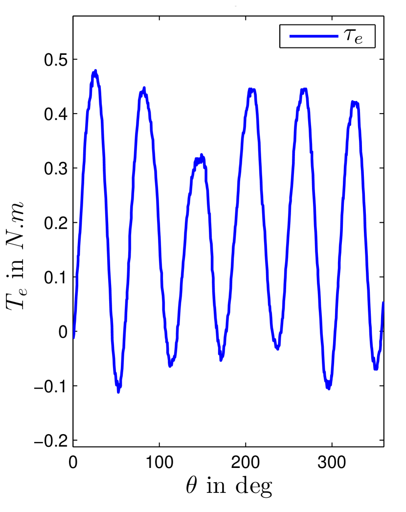
(a) SPM torque measurement

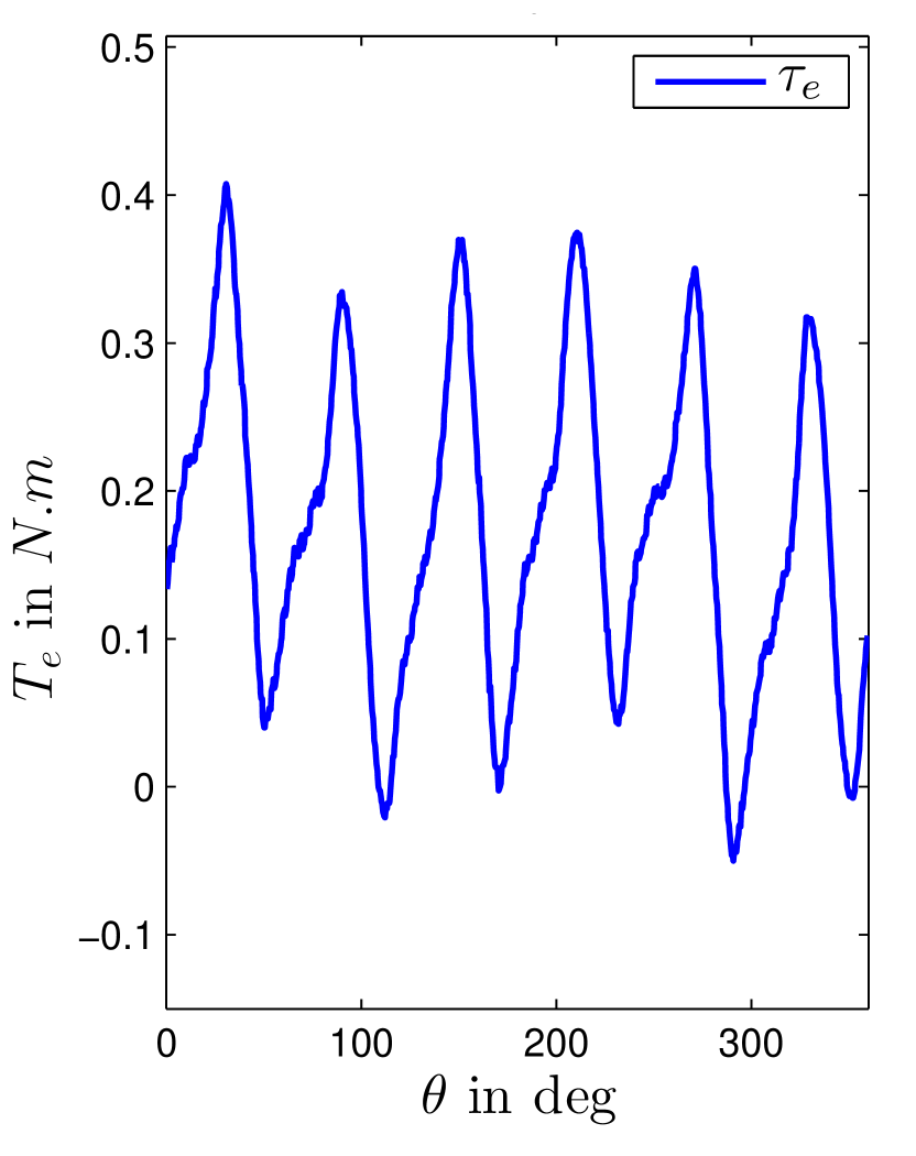
(b) IPM torque measurement

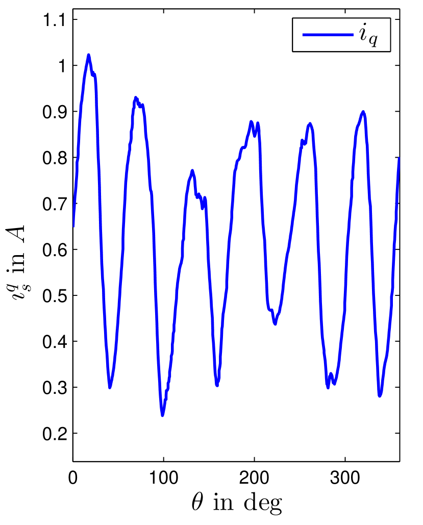
(c) SPM current $\imath_{s}^{q}$ measurement

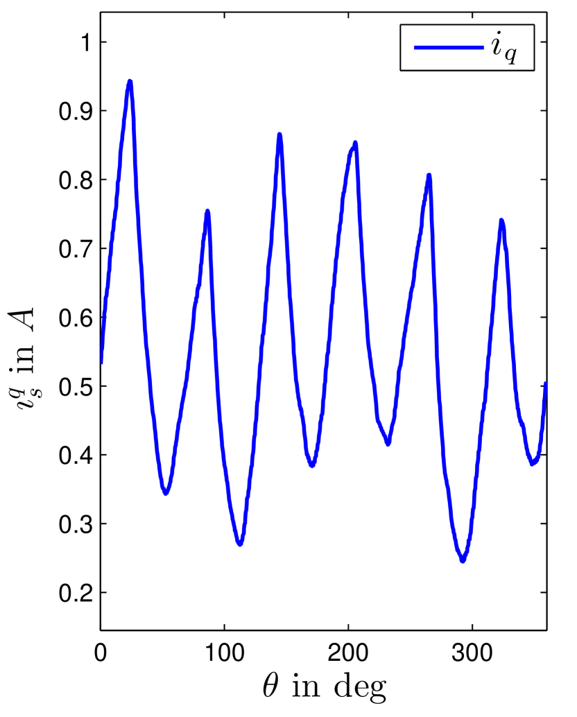
(d) IPM current $\imath_{s}^{q}$ measurement

Figure 2: Stator current and torque measurements diverse kinds of PMSM

Moreover if we consider the $0$-axis, the symmetries III-A implies $\mathcal{H}^{dq0}$ hence $\phi_{s}^{0}$ is only $\frac{2\pi}{3}$-periodic with respect to $\theta$. This effect can be experimentally seen on the potential $v_{N}$ of the point $O$ in figure 1, thanks to (27)

$$\frac{d\phi_{s}^{0}}{dt}(\theta,\rho,\phi_{s}^{dq})=u_{s}^{0}=v_{s}^{0}-\sqrt{3}v_{N};$$

here $v_{s}^{0}:=\frac{1}{\sqrt{3}}(v_{s}^{a}+v_{s}^{b}+v_{s}^{c})$ is as usual set to $0$ by the inverter. Therefore $v_{N}$ will exhibit a $\frac{2\pi}{3}$-periodicity with respect to $\theta$, which was also measured on the test bench.

V Modeling of magnetic saturation

We now investigate the effect of magnetic saturations; this very important when trying to control the motor at low velocity and high load, see e.g. [1, 2, 3, 4]. We consider only sinusoidal motors (i.e. the energy function $\mathcal{H}^{dq}$ is independent of $\theta$) since the non-sinusoidal effects in well-wound PMSMs are experimentally small in the presence of magnetic saturation. We still assume the magnetic energy does not depend on the kinetic momentum $\rho$, and the simplest possible kinetic energy.

In normal operation $\phi_{s}^{d}$ is close to the permanent magnet flux $\phi_{M}$, while $\phi_{s}^{q}$ is small with respect to $\phi_{M}$. It is thus natural to expand $\mathcal{H}^{dq}$ as a Taylor series in the variables $(\phi_{s}^{d}-\phi_{M})$ and $\phi_{s}^{q}$

$$\mathcal{H}^{dq}=\mathcal{H}_{l}^{dq}+\sum\limits_{n=3}^{\infty}\sum\limits_{k=0}^{n}\alpha_{n-k,k}(\phi_{s}^{d}-\phi_{M})^{n-k}{\phi_{s}^{q}}^{k},$$ (47)

where $\mathcal{H}_{l}^{dq}$ is given by (42). Moreover, all odd powers of $\phi_{s}^{q}$ have by (40a) null coefficients, hence

$$\mathcal{H}^{dq}=\mathcal{H}_{l}^{dq}+\sum\limits_{n=3}^{\infty}\sum\limits_{m=0}^{\lfloor\frac{n}{2}\rfloor}\alpha_{n-2m,2m}(\phi_{s}^{d}-\phi_{M})^{n-2m}{\phi_{s}^{q}}^{2m}.$$ (48)

We experimentally checked the validity of this conclusion on the two motors described in table I. We first obtained the flux-current relation by integrating the back-electromotive force when applying voltage steps, see figure 3. We then truncated the series at $n=4$ and experimentally identified $L^{d},L^{q},\alpha_{3,0},\alpha_{1,2},\alpha_{4,0},\alpha_{2,2},\alpha_{0,4}$, see [18] for details. The agreement between the flux-current relation obtained from $\mathcal{H}^{dq}$ and the experimental flux-current relation is excellent. Notice the linear model using only $\mathcal{H}_{l}^{dq}$ is good only at low current.

Motor	IPM	SPM
Measured $R_{s}$	$1.52\Omega$	$2.1\Omega$
$\frac{\phi_{M}^{2}}{L^{d}}$	$4.20\pm 0.12A.Wb$	$3.06\pm 0.08A.Wb$
$\frac{\phi_{M}^{2}}{L^{q}}$	$2.83\pm 0.12A.Wb$	$2.94\pm 0.08A.Wb$
$\phi_{M}^{3}\alpha_{3,0}$	$0.770\pm 0.007A.Wb$	$0.655\pm 0.006A.Wb$
$\phi_{M}^{3}\alpha_{1,2}$	$0.702\pm 0.009A.Wb$	$0.617\pm 0.010A.Wb$
$\phi_{M}^{4}\alpha_{4,0}$	$0.486\pm 0.012A.Wb$	$0.724\pm 0.010A.Wb$
$\phi_{M}^{4}\alpha_{2,2}$	$0.734\pm 0.015A.Wb$	$1.010\pm 0.025A.Wb$
$\phi_{M}^{4}\alpha_{0,4}$	$0.175\pm 0.004A.Wb$	$0.262\pm 0.006A.Wb$

Table II: Experimental magnetic parameters

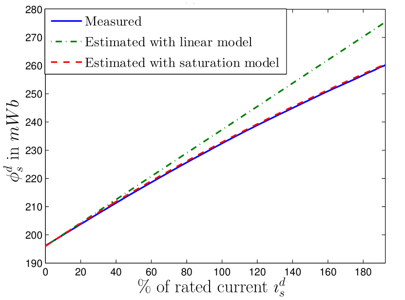
(a) IPM motor

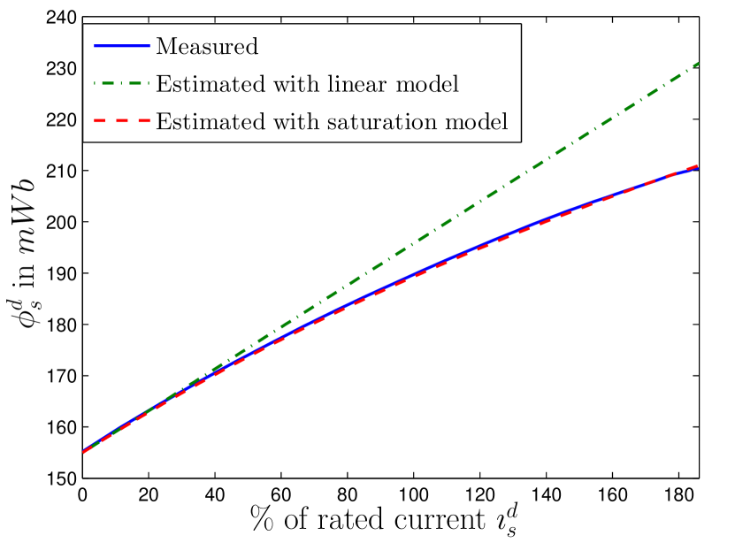
(b) SPM motor

Figure 3: Experimental and fitted flux-current relations.

VI Energy-based modeling for the induction motor

We now apply our approach to the Induction Motor (IM). We show that taking the most basic assumptions (sinusoidal and linear motor) we find again the linear model as we did in section III-E.

VI-A Deploying the formalism

Assuming the squirrel-cage rotor is actually equivalent to three identical wound phases, the generalized coordinates of an IM with three identical stator windings are

$$q={(\theta,q_{s}^{a},q_{s}^{b},q_{s}^{c},q_{r}^{a},q_{r}^{b},q_{r}^{c})}^{T},$$

where $\theta$ is the (electrical) rotor angle and $q_{s}^{abc}$ and $q_{r}^{abc}$ are the electrical charges in the stator and rotor windings respectively. Their derivatives are

$$\dot{q}={(\omega,\imath_{s}^{a},\imath_{s}^{b},\imath_{s}^{c},\imath_{r}^{a},\imath_{r}^{b},\imath_{r}^{c})}^{T},$$

where $\omega$ is the (electrical) rotor velocity and $\imath_{s}^{abc}$ and $\imath_{r}^{abc}$ are the currents in stator and rotor windings respectively. Proceeding as in II-C, the generalized momenta are

$$p={(\rho,\phi_{s}^{a},\phi_{s}^{b},\phi_{s}^{c},\phi_{r}^{a},\phi_{r}^{b},\phi_{r}^{c})}^{T},$$

where $\rho$ is the kinetic momentum and $\phi^{abc}$ and $\phi_{r}^{abc}$ are the flux produced by stator and rotor windings respectively. The power exchanges are:

• the electrical power ${u_{s}^{abc}}^{T}\imath_{s}^{abc}$ provided to the motor by the electrical source, where $u_{s}^{abc}$ is the vector of voltage drops along the stator winding; this power is associated with the generalized force $u_{s}^{abc}$

• the electrical power $-R_{s}{\imath_{s}^{abc}}^{T}\imath_{s}^{abc}$ dissipated in the stator resistances $R_{s}$; it is associated with the generalized force $-R_{s}\imath_{s}^{abc}$.

• the electrical power $-R_{r}{\imath_{r}^{abc}}^{T}\imath_{r}^{abc}$ dissipated in the rotor resistances $R_{r}$; it is associated with the generalized force $-R_{r}\imath_{r}^{abc}$.

• the mechanical power $-T_{L}\frac{\omega}{n}$ dissipated in the load, where $T_{L}$ is the load torque and $n$ the number of pole pairs; it is associated with the generalized force $-T_{L}$.

Using the same method as in II-C, we find

$$\frac{d\phi_{s}^{abc}}{dt} = u_{s}^{abc}-R_{s}\imath_{s}^{abc}$$ (49a)

$$\frac{d\phi_{r}^{abc}}{dt} = -R_{r}\imath_{r}^{abc}$$ (50a)

$$n\frac{d\rho}{dt} = T_{e}^{abc}-T_{L},$$ (51a)

where the stator variables are expressed in the stator frame and the rotor variables are expressed in the rotor frame. The current-flux and electro-mechanical relations are also similar,

$$\imath_{s}^{abc}(\theta,\rho,\phi_{s}^{abc},\phi_{r}^{abc}) := \frac{\partial\mathcal{H}^{abc}}{\partial\phi_{s}^{abc}}(\theta,\rho,\phi_{s}^{abc},\phi_{r}^{abc})$$ (52)

$$\imath_{r}^{abc}(\theta,\rho,\phi_{s}^{abc},\phi_{r}^{abc}) := \frac{\partial\mathcal{H}^{abc}}{\partial\phi_{r}^{abc}}(\theta,\rho,\phi_{s}^{abc},\phi_{r}^{abc})$$ (53)

$$T_{e}^{abc}(\theta,\rho,\phi_{s}^{abc},\phi_{r}^{abc}) := -n\frac{\partial\mathcal{H}^{abc}}{\partial\theta}(\theta,\rho,\phi_{s}^{abc},\phi_{r}^{abc}).$$ (54)

Due to the connection scheme of the rotor,

$$\imath_{r}^{a}+\imath_{r}^{b}+\imath_{r}^{c}=0$$ (55)

and the fact that most stators are star-connected (see figure 1), it is still interesting to change frame and decouple the $0$-axis as was done in II-D. It is also interesting to express all the variables in the same frame rotating at the synchronous speed $\omega_{s}$. To do so we define $x_{s}^{dq0}:={\mathcal{K}(\theta_{s})}^{T}x_{s}^{abc}$ and $x_{r}^{dq0}:={\mathcal{K}(\theta_{s}-\theta)}^{T}x_{r}^{abc}$ where $\frac{d\theta_{s}}{dt}:=\omega_{s}$ and

$$\mathcal{K}(\theta):=\sqrt{\frac{2}{3}}\begin{pmatrix}\operatorname{cos}\theta&\operatorname{cos}\theta-\frac{2}{3}&\operatorname{cos}\theta-\frac{4}{3}\\ -\operatorname{sin}\theta&-\operatorname{sin}\theta-\frac{2}{3}&-\operatorname{sin}\theta-\frac{4}{3}\\ \frac{1}{\sqrt{2}}&\frac{1}{\sqrt{2}}&\frac{1}{\sqrt{2}}\\ \end{pmatrix}$$

Even through the equation will not be preserved, as in II-E, we can get similar relations

$$\frac{d\phi_{s}^{dq}}{dt} = u_{s}^{dq}-R_{s}\imath_{s}^{dq}-\mathcal{J}\omega_{s}\phi_{s}^{dq}$$ (56a)

$$\frac{d\phi_{r}^{dq}}{dt} = -R_{r}\imath_{r}^{dq}-\mathcal{J}(\omega_{s}-\omega)\phi_{r}^{dq}$$ (57a)

$$n\frac{d\rho}{dt} = T_{e}^{dq}-T_{L}$$ (58a)

These are the usual dynamic equations for the IM (see e.g. [5, 6]).

In the $dq$ frame the current-flux and electromechanical relations then read

$$\imath_{s}^{dq}(\theta,\rho,\phi_{s}^{dq},\phi_{r}^{dq}) := \frac{\partial\mathcal{H}^{dq}}{\partial\phi_{s}^{dq}}(\theta,\rho,\phi_{s}^{dq},\phi_{r}^{dq})$$ (59)

$$\imath_{r}^{dq}(\theta,\rho,\phi_{s}^{dq},\phi_{r}^{dq}) := \frac{\partial\mathcal{H}^{dq}}{\partial\phi_{r}^{dq}}(\theta,\rho,\phi_{s}^{dq},\phi_{r}^{dq})$$ (60)

$$T_{e}^{dq}(\theta,\rho,\phi_{s}^{dq},\phi_{r}^{dq}) := -n\frac{\partial\mathcal{H}^{dq}}{\partial\theta}+n{\imath_{r}^{dq}}^{T}\mathcal{J}\phi_{r}^{dq}.$$ (61)

VI-B Symmetries

We now use the motor construction symmetries as in section III considering only the case of a sinusoidal induction machine.

So, whatever the angle $\theta$ of the rotor, the energy will be the same, as long as the relative position of the rotor flux space vector with respect to stator flux space vector remains the same. Thus the energy function in the $dq$ frame does not depend on $\theta$.

Rotating the stator and rotor flux space vectors by the same angle $\eta$ preserves the energy, so

$$\mathcal{H}^{dq}(\rho,\phi_{s}^{dq},\phi_{r}^{dq})=\mathcal{H}^{dq}(\rho,\mathcal{R}(\eta)\phi_{s}^{dq},\mathcal{R}(\eta)\phi_{r}^{dq}).$$ (62)

Exchanging two phases on the stator and the rotor and symmetrizing the rotor position also preserves the energy so

$$\mathcal{H}^{dq}(\rho,\phi_{s}^{dq},\phi_{r}^{dq})=\mathcal{H}^{dq}(-\rho,\mathcal{S}\phi_{s}^{dq},\mathcal{S}\phi_{r}^{dq}),$$ (63)

with

$$\mathcal{S}:=\begin{pmatrix}1&0\\ 0&-1\end{pmatrix}.$$

VI-C The linear sinusoidal model

We consider a second order-polynomial energy function independent on $\theta$ and with magnetic part independent on $\rho$. We keep the simplest expression of the kinetic energy. Such a model is of the form

$$\mathcal{H}_{l}^{dq} := \frac{1}{2Jn^{2}}\rho^{2}+a+b\phi_{s}^{dq}+c\phi_{r}^{dq}$$ (64)

$$+ {\phi_{s}^{dq}}^{T}D\phi_{s}^{dq}+{\phi_{s}^{dq}}^{T}E\phi_{r}^{dq}+{\phi_{r}^{dq}}^{T}F\phi_{r}^{dq},$$

where $a\in\mathbb{R}$, $(b,c)\in(\mathbb{R}^{2})^{2}$ and $(D,E,F)\in(\mathcal{M}_{2}(\mathbb{R}))^{3}$.

The equation (62) implies that $b=c=(0,0)$ and $D$, $E$ and $F$ commute with the rotations. So $(D,E,F)\in\left\{\alpha\mathcal{I}+\beta\mathcal{J},(\alpha,\beta)\in\mathbb{R}^{2}\right\}$ where $\mathcal{I}\in\mathcal{M}_{2}(\mathbb{R})$ is the identity matrix and $\mathcal{J}$ was defined in II-E. Due to (63) $D$, $E$ and $F$ are colinear with $\mathcal{I}$ because $\mathcal{J}$ does not commute with $\mathcal{S}$, hence the energy function is of the form

$$\mathcal{H}_{l}^{dq}:=\frac{1}{2Jn^{2}}\rho^{2}+a+d{\phi_{s}^{dq}}^{T}\phi_{s}^{dq}+e{\phi_{s}^{dq}}^{T}\phi_{r}^{dq}+f{\phi_{r}^{dq}}^{T}\phi_{r}^{dq}.$$ (65)

We can choose freely $a=0$ as the energy function is defined up to a constant. We define $\sigma$, $L_{m}$, $L_{s}$ and $L_{r}$ by the implicit relations (it can be checked that it is invertible when it is defined)

$$L_{r}L_{s}\sigma=L_{s}L_{r}-L_{m}^{2}$$

$$d=\frac{1}{2L_{s}\sigma}\qquad e=-\frac{2L_{m}}{2L_{r}L_{s}\sigma}\qquad f=\frac{1}{2L_{r}\sigma}$$

Thus, the energy function reads

$$\mathcal{H}^{dq} := \frac{1}{2Jn^{2}}\rho^{2}+\frac{L_{m}}{2L_{s}L_{r}\sigma}{(\phi_{s}^{dq}-\phi_{r}^{dq})}^{T}(\phi_{s}^{dq}-\phi_{r}^{dq})$$ (66)

$$+ \frac{L_{r}-L_{m}}{2L_{s}L_{r}\sigma}{\phi_{s}^{dq}}^{T}\phi_{s}^{dq}+\frac{L_{s}-L_{m}}{2L_{s}L_{r}\sigma}{\phi_{r}^{dq}}^{T}\phi_{r}^{dq}.$$

Applying (59) and (60) one gets the current-flux relations

$$L_{s}L_{r}\sigma\imath_{s}^{dq}=L_{m}(\phi_{s}^{dq}-\phi_{r}^{dq})+(L_{r}-L_{m})\phi_{s}^{dq}$$

$$L_{s}L_{r}\sigma\imath_{r}^{dq}=L_{m}(\phi_{r}^{dq}-\phi_{s}^{dq})+(L_{s}-L_{m})\phi_{r}^{dq}.$$

Inverting these equations and taking into account the electro-mechanical torque is $T_{e}=n{\imath_{r}^{dq}}^{T}\mathcal{J}\phi_{s}^{dq}$, the usual relations (see e.g. [5, 6]) are easily identified. Therefore we recovered the linear sinusoidal model for the IM without the tedious microscopic approach.

References

- [1] N. Bianchi, E. Fornasiero, and S. Bolognani, “Effect of stator and rotor saturation on sensorless rotor position detection,” in Energy Conversion Congress and Exposition (ECCE), 2011 IEEE, 2011, pp. 1528–1535.
- [2] F. M. L. L. De Belie, J. A. A. Melkebeek, L. Vandevelde, R. Boel, K. Geldhof, and T. Vyncke, “A nonlinear model for synchronous machines to describe high-frequency signal based position estimators,” in Electric Machines and Drives, 2005 IEEE International Conference on, 2005, pp. 696–703.
- [3] D. Reigosa, P. Garcia, D. Raca, F. Briz, and R. Lorenz, “Measurement and adaptive decoupling of cross-saturation effects and secondary saliencies in sensorless-controlled IPm synchronous machines,” in Industry Applications Conference, 2007. 42nd IAS Annual Meeting. Conference Record of the 2007 IEEE, 2007, pp. 2399–2406.
- [4] P. Sergeant, F. De Belie, and J. Melkebeek, “Effect of rotor geometry and magnetic saturation in sensorless control of pm synchronous machines,” Magnetics, IEEE Transactions on, vol. 45, no. 3, pp. 1756–1759, 2009.
- [5] J. Chiasson, Modeling and high performance control of electric machines. Wiley-IEEE Press, 2005, vol. 24.
- [6] P. Krause, O. Wasynczuk, and S. Sudhoff, Analysis of Electrical Machinery and Drive Systems, 2nd ed. Wiley-IEEE Press, 2002.
- [7] N. Bianchi and S. Bolognani, “Design techniques for reducing the cogging torque in surface-mounted pm motors,” Industry Applications, IEEE Transactions on, vol. 38, no. 5, pp. 1259–1265, Sep 2002.
- [8] V. Petrovic, R. Ortega, A. Stankovic, and G. Tadmor, “Design and implementation of an adaptive controller for torque ripple minimization in pm synchronous motors,” Power Electronics, IEEE Transactions on, vol. 15, no. 5, pp. 871–880, Sep 2000.
- [9] Z. Zhu and D. Howe, “Analytical prediction of the cogging torque in radial-field permanent magnet brushless motors,” Magnetics, IEEE Transactions on, vol. 28, no. 2, pp. 1371–1374, Mar 1992.
- [10] E. Levi, “Saturation modelling in d-q axis models of salient pole synchronous machines,” Energy Conversion, IEEE Transactions on, vol. 14, no. 1, pp. 44–50, Mar 1999.
- [11] B. Stumberger, G. Stumberger, D. Dolinar, A. Hamler, and M. Trlep, “Evaluation of saturation and cross-magnetization effects in interior permanent-magnet synchronous motor,” Industry Applications, IEEE Transactions on, vol. 39, no. 5, pp. 1264–1271, Sept 2003.
- [12] J. Melkebeek and J. Willems, “Reciprocity relations for the mutual inductances between orthogonal axis windings in saturated salient-pole machines,” Industry Applications, IEEE Transactions on, vol. 26, no. 1, pp. 107–114, Jan 1990.
- [13] E. Whittaker, A Treatise on the Analytical Dynamics of Particules and Rigid Bodies (4th edition). Cambridge University Press, Cambridge, 1937.
- [14] L. Landau and E. Lifshitz, Mechanics, 4th ed. Mir, Moscow, 1982.
- [15] D. C. White and H. H. Woodson, Electromechanical energy conversion. Wiley, 1959.
- [16] R. Ortega, Passivity-based control of Euler-Lagrange systems: mechanical, electrical and electromechanical applications. Springer, 1998.
- [17] P. Nicklasson, R. Ortega, G. Espinosa-Perez, and C. G. J. Jacobi, “Passivity-based control of a class of blondel-park transformable electric machines,” Automatic Control, IEEE Transactions on, vol. 42, no. 5, pp. 629–647, May 1997.
- [18] A. Jebai, F. Malrait, P. Martin, and P. Rouchon, “Estimation of saturation of permanent-magnet synchronous motors through an energy-based model,” in IEEE International Electric Machines Drives Conference, 2011, pp. 1316 –1321.