The secular evolution of the Kuiper belt after a close stellar encounter
Abstract
We show the effects of the perturbation caused by a passing by star on the Kuiper belt objects (KBOs) of our Solar System. The dynamics of the Kuiper belt (KB) is followed by direct -body simulations. The sampling of the KB has been done with up to , setting the KBOs on initially nearly circular orbits distributed in a ring of surface density . This modelization allowed us to investigate the secular evolution of the KB upon the encounter with the perturbing star. Actually, the encounter itself usually leads toward eccentricity and inclination distributions similar to observed ones, but tends also to excite the low-eccentricity population ( around from the Sun), depleting this region of low eccentricities. The following long-term evolution shows a “cooling” of the eccentricities repopulating the low-eccentricity area. In dependence on the assumed KBO mass spectrum and sampled number of bodies, this repopulation takes place in a time that goes from 0.5 Myr to 100 Myr. Due to the unavoidable limitation in the number of objects in our long-term simulations (), we could not consider a detailed KBO mass spectrum, accounting for low mass objects, thus our present simulations are not reliable in constraining correlations among inclination distribution of the KBOs and other properties, such as their size distribution. However, our high precision long term simulations are a starting point for future larger studies on massively parallel computational platforms which will provide a deeper investigation of the secular evolution (Myr) of the KB over its whole mass spectrum.
keywords:
Kuiper belt: general; methods: numerical; planets and satellites: dynamical evolution and stability.MNRAS Accepted 2014 August 11th. Received 2014 July 14th; in original form 2014 March 21th.
1 Introduction
The Solar System is hedged by a ring composed of a huge number of small bodies: the Edgeworth-Kuiper belt (Jewitt & Luu, 1993) (hereafter briefly called Kuiper belt, or KB). The Kuiper belt bears the signature it the early evolution of the Solar System, and a contains records of the end-state of the accretion processes occurred in that region. Therefore, the knowledge of the history of the Kuiper belt objects (KBOs) is relevant to be able to develop a full consensus of the formation of the Solar System.
The majority of the KBOs are located between about 30 and 90 from the Sun, but most are around the 2:3 resonance with Jupiter, at 39.5 and at its 1:2 resonance, roughly around 48 . The total mass is estimated from to M⊕ (Luu & Jewitt, 2002). There are several, indirect, arguments suggesting that this is just a small fraction of its initial mass because most of it has been lost (see Kenyon & Luu (1999)). The size distribution of the KBOs is, usually, assumed as a power law , where and are constants. The exponent is estimated (Bernstein et al., 2004; Fraser & Kavelaars, 2009). For a more detailed description of the Kuiper belt we refer, e.g., to Luu & Jewitt (2002).
The KB has a bimodal inclination distribution resulting of two separate populations (Brown, 2001). The dynamically cold population refers to objects moving on almost planar orbits with relatively low inclinations (up to about 10∘) respect to the ecliptic. On the other side, the dynamically hot population is characterized by highly inclined orbits (up to 40∘) with respect to the ecliptic. Note that these two populations are different from what we call, in this paper, the low-eccentricity population, which are objects on nearly circular orbits (orbital eccentricities ) and the high-eccentricity population (eccentricities 0.1.
In Fig. 1 the eccentricities and inclinations are plotted as function of the semi-major axis for KBOs observed from the Minor Planet Center (MPC) (Marsden, 1980) which is the center of the Smithsonian Astrophysical Observatory (SAO) dedicated to tracking, monitoring, calculating and disseminating data from asteroids and comets.
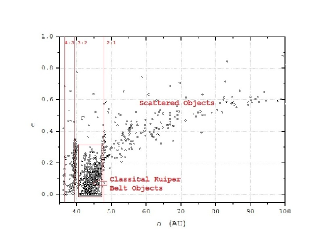
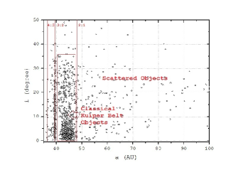
The KBOs have been sub-categorized in three groups:
-
1.
classical KBOs ( , , );
-
2.
scattered KBOs ( , , );
-
3.
main resonant KBOs :
-
•
4:3 resonance (, , );
-
•
3:2 resonance, Plutino’s (, ,);
-
•
2:1 resonance (, , ).,
-
•
where semimajor axes, , are in .
These sub-populations have been explain through a phase of planet migration and a phase of clearing of the environment during the evolution of the early Solar System Malhotra (1993, 1995). In the latter phase the resonance population was formed by sweeping resonance capture in which the Jovian planets withstand considerable orbital migration as a result of encounters with residual planetesimals. While Neptune moved outwards, a small body like Pluto in an initially circular orbit could have been captured into the 3:2 resonance. The high orbital eccentricity would subsequently be induced by repeated orbital crossings with Neptune.
Many others studies have attempted to better understand the properties of the KBOs. Gomes (2003) investigated how the outward migration of Neptune, as proposed by Malhotra (1993, 1995), could have scattered objects from onto high- orbits leading to the current classical Kuiper belt region. He concluded that the high- population was formed closer to the Sun and brought into the classical Kuiper belt during planetary migration, whereas the cold population represents a primordial, relatively undisturbed population. This also led to the speculation that other mechanisms, such as planetary migration, have been the cause of the correlation between inclinations and colors in the classical Kuiper belt rather than environmental effects like the collisions among the KBOs (see Doressoundiram et al. (2008)). Detailed discussions about the correlation of the inclination with the color, size and binary of the KBOs are given by Levison & Stern (2001); Brucker et al. (2009); Noll et al. (2008); Volk & Malhotra (2011). More recently a model, called the Nice model, has been proposed (Levison et al., 2008), which argues that the giant planets migrated from an initial compact configuration into their present orbits, long after the dissipation of the initial protoplanetary gas disk. The Nice model seems to provide a acceptable explanation for the formation of the classical and scattered populations, and for the correlation between inclinations and colors (for more detail see Levison et al. (2008)). The Nice model, however, predicts a higher eccentricities in classical KBO orbits than is observed.
An interaction between a passing field star and the the Solar System could also be responsible for some of the orbital families observed in the KBO, which is the main topic of this paper.
2 The fly-by star perturbation and the -body scheme
An encounter between a passing star and the Solar System is quite likely, considering that the Solar System was probably formed in an open star cluster (Portegies Zwart, 2009). The hypothesis of a closely passing star has been hypothesized before, and used to explain KBO families (Ida et al., 2000; Kobayashi & Ida, 2001; Kobayashi et al., 2005; Melita et al., 2005; Malmberg et al., 2011). The cost of such calculations, however, prevented earlier research on the secular evolution of the KBO by mean of high resolution simulations.
We focus our attention on the investigation of the effects of the long-term evolution of the Kuiper belt after a close stellar encounter on the structure of the Kuiper belt. We adopt a direct -body treatment in which the mutual, pair-wise, interactions between KBOs, planets and stars are taken into account self-consistently. Due to the computational expense of this method we are limited to about total bodies.
We modeled the early Solar System as composed by the Sun, the eight major planets, Pluto and the Kuiper belt. Each object was considered a point-mass; we did not account for collisions. The KBOs were initially moving in circular orbits in a flat ring in the plane of the ecliptic. This corresponds to an initially cold population, without a component in their motion. We adopted a surface density , where is the heliocentric distance (see Holman (1995)).
We studied two possible configurations:
-
•
(i) model A, with a radial extension in the range from to and four different values of the total mass of the KB, M⊕;
-
•
(ii) model B, with a radial extension in the range from to and a total mass M⊕.
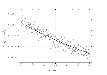
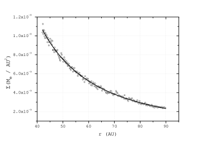
The mass function of the KBOs was derived from the conversion in mass of the size () distribution, assuming a constant KBO density (i.e. kg/m3), which results in with a cut at M⊕ (corresponding to km) and M⊕ (corresponding to km). In Fig. 2 we present the surface density of the models A and B as a function of the heliocentric distance for KBOs with the same individual mass, . Here is the total mass of the Kuiper belt and the number of KBOs. With this choice we have a good sampling of the KB without an exceedingly large number () of particles.
We integrate the equations of motion by direct summation -body codes running on Graphics Processing Units (GPUs). For the gravitational -body problem these accelerators give a manifold speed increase with respect to code running on CPU (Nyland et al., 2007; Portegies Zwart et al., 2007; Bédorf & Portegies Zwart, 2012). Parallel computers equipped more than one hundred GPUs have been utilized for various studies (Capuzzo-Dolcetta et al., 2013; Capuzzo-Dolcetta & Spera, 2013; Berczik et al., 2011, 2013) have been run efficiently in parallel to provide the computational power necessary to perform direct many body simulations. Access to such large GPU-equipped supercomputers, however, is not easy, in particular when the computations required a considerable fraction of the available hardware. We therefore mainly ran our simulation on the Little Green Machine, a at the Sterrewacht Leiden built dedicated GPU-equipped supercomputer, specifically built for performing GPU-related calculations. Even with this machine, we had to limit the number of bodies to about a hundred thousand, but we performed several simulations (of models A and B) for each realization of the initial conditions in order to assure that the results of our calculations were not a statistical anomaly. Recently Portegies Zwart & Boekholt (2014) demonstrated that performing multiple simulations with the same initial conditions provide a statistically correct sampling of the real solutions. In these runs we varied the mass, impact parameter and the inclination of the incoming star.
| (1) |
where are in and velocities in km/s. The system of reference was centered on the Sun, and the impact parameters and inclination characterize the orbit of the encountering star. The incoming star was placed in a ring of radius at a distance of 500 in the -direction parallel to the plane. In Tab. 1 we present the initial conditions for our simulations. In order to have a full coverage of the parameter space, and should be varied as free parameters. However, a systematic set of body simulations is computational expensive (at least when considering large enough to guarantee a good sampling) forced us to reduce the investigation in the parameter space. Consequently, we considered that the most relevant thing to do was exploring the role of the initial spatial coordinates. Actually, the variation of two free parameters are enough for exploring encounters with different strength (see Sect. 3). Of course, a more extended study of the other free parameters could allow a wider comprehension of the role of stellar encounters on the KB structure.
| index | index | ||||||||
| 1 | 140 | 90 | 0.000 | 140.000 | 33 | 200 | 30 | 173.205 | 100.000 |
| 2 | 140 | 100 | -24.311 | 137.873 | 34 | 200 | 60 | 100.000 | 173.205 |
| 3 | 140 | 110 | -47.883 | 131.557 | 35 | 200 | 70 | 68.404 | 187.939 |
| 4 | 150 | 30 | 129.904 | 75.000 | 36 | 200 | 75 | 51.764 | 193.185 |
| 5 | 150 | 60 | 75.000 | 129.904 | 37 | 200 | 80 | 34.730 | 196.962 |
| 6 | 150 | 90 | 0.000 | 150.000 | 38 | 200 | 90 | 0.000 | 200.000 |
| 7 | 150 | 100 | -26.047 | 147.721 | 39 | 200 | 105 | -51.764 | 193.185 |
| 8 | 150 | 110 | -51.303 | 140.954 | 40 | 200 | 120 | -100.000 | 173.205 |
| 9 | 150 | 120 | -75.000 | 129.904 | 41 | 200 | 135 | -141.421 | 141.421 |
| 10 | 150 | 150 | -129.904 | 75.000 | 42 | 200 | 150 | -173.205 | 100.000 |
| 11 | 160 | 90 | 0.000 | 160.000 | 43 | 212.5 | 60 | 106.250 | 184.030 |
| 12 | 160 | 100 | -27.784 | 157.569 | 44 | 212.5 | 75 | 54.999 | 205.259 |
| 13 | 160 | 110 | -54.723 | 150.351 | 45 | 212.5 | 90 | 0.000 | 212.500 |
| 14 | 170 | 90 | 0.000 | 170.000 | 46 | 212.5 | 105 | -54.999 | 205.259 |
| 15 | 170 | 100 | -29.520 | 167.417 | 47 | 212.5 | 120 | -106.250 | 184.030 |
| 16 | 170 | 110 | -58.143 | 159.748 | 48 | 212.5 | 135 | -150.260 | 150.260 |
| 17 | 170 | 90 | 0.000 | 170.000 | 49 | 212.5 | 150 | -184.030 | 106.250 |
| 18 | 170 | 100 | -29.520 | 167.417 | 50 | 225 | 30 | 194.856 | 112.500 |
| 19 | 170 | 110 | -58.143 | 159.748 | 51 | 225 | 60 | 112.500 | 194.856 |
| 20 | 175 | 30 | 151.554 | 87.500 | 52 | 225 | 75 | 58.234 | 217.333 |
| 21 | 175 | 60 | 87.500 | 151.554 | 53 | 225 | 90 | 0.000 | 225.000 |
| 22 | 175 | 70 | 59.854 | 164.446 | 54 | 225 | 105 | -58.234 | 217.333 |
| 23 | 175 | 80 | 30.388 | 172.341 | 55 | 225 | 120 | -112.500 | 194.856 |
| 24 | 175 | 90 | 0.000 | 175.000 | 56 | 225 | 135 | -159.099 | 159.099 |
| 25 | 175 | 120 | -87.500 | 151.554 | 57 | 225 | 150 | -194.856 | 112.500 |
| 26 | 175 | 150 | -151.554 | 87.500 | 58 | 237.5 | 60 | 118.750 | 205.681 |
| 27 | 180 | 70 | 61.564 | 169.145 | 59 | 237.5 | 75 | 61.470 | 229.407 |
| 28 | 180 | 80 | 31.257 | 177.265 | 60 | 237.5 | 90 | 0.000 | 237.500 |
| 29 | 180 | 90 | 0.000 | 180.000 | 61 | 237.5 | 105 | -61.470 | 229.407 |
| 30 | 190 | 70 | 64.984 | 178.542 | 62 | 237.5 | 120 | -118.750 | 205.681 |
| 31 | 190 | 80 | 32.993 | 187.113 | 63 | 237.5 | 135 | -167.938 | 167.938 |
| 32 | 190 | 90 | 0.000 | 190.000 | 64 | 237.5 | 150 | -205.681 | 118.750 |
Calculations were performed using the direct summation code HiGPUs (Capuzzo-Dolcetta et al., 2013), which is publicly available via the Astronomical Multipurpose Software Environment (AMUSE) (Portegies Zwart et al., 2009; Pelupessy et al., 2013; Portegies Zwart et al., 2013).
This code uses its own kernels to implement at best a 6th-order Hermite’s integrator (Nitadori & Makino, 2008) with block time-steps (Aarseth, 2003) method.
We tested the accuracy of HiGPUs in getting the results of interest here through comparison with two symplectic -body codes, NBSymple (Capuzzo-Dolcetta et al., 2011), which is based on a symplectic second and sixth order method for the time integration of the equations of motion and HUAYNO (Pelupessy et al., 2012), which uses recursive-Hamiltonian splitting to generate multiple-timestep integrators that conserve momentum to machine precision. The comparison indicates as fully reliable the simulations done with the (much faster) HiGPUs code.
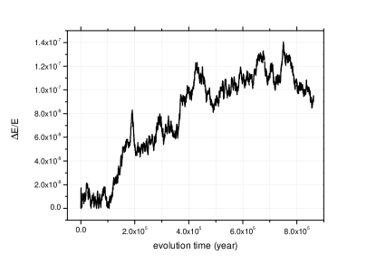
All the simulations were performed using a softening parameter, , in the pairwise Newtonian potential , where is the to particle distance. The value was set to , which is times smaller than the initial average distance to the nearest neighbour in our sampling, and times bigger than the radius of Pluto. This choice guarantees the preservation of the newtonian behaviour of the interobject force while keeping under control spurious fluctuations over the mean field (see following Subsect. 2.1). The maximum time step for the hierarchical block time steps was . The energy conservation was checked along the system evolution by its fractional time variation defined as
| (2) |
At the end of the simulations it was always below the value , which is more than sufficient to assure that we statistically correctly sample the result of a true (converged) solution to the -body problem (Portegies Zwart & Boekholt, 2014).
2.1 The role of softening
The real KB is likely composed of various thousands objects. The study of the secular evolution of the KB with a high-precision, direct summation, -body code after the encounter with a passing-by star is out of reach with our available hardware. For this reason, to represent the KBOs we limited to values of just below , taking as reference value (ten bodies represent the incoming star, the Sun and the planets) which showed to be a good compromise between accuracy (resolution) and computational speed. Of course, to give physical reliability to our results obtained by such subsampling, we needed the introduction of a softening parameter (, as described above) whose size must be calibrated. Actually, the role of softening parameter in the N-body simulation is a long, highly debated question. It is well known that a softening parameter in the Newtonian particle-particle force has the double role of i) avoiding the ultraviolet singularity in the closest interaction and ii) reducing the spurious granularity effects induced by the use of a sub sampled N-body set of particles to reproduce the evolution of a large stellar system. The choice of the softening length, , is characterized by a proper balance between the width of the softening length, to be small enough to preserve the Newtonian behaviour and, at the same time, large enough to avoid spurious collisionally in the evolutionary behaviour of the system. To fulfil the second requirement above, is necessarily much larger than the average KBO radius but this is not a serious issue because the average close neighbour distance, , in the simulated KB system is the average KB radius. On the other hand, the first requirement above (preserve Newtonian behaviour of the force) requires an sufficiently smaller than . Actually, we tested the simulations with two values of the softening ( and for ), which are both significantly smaller than which is for . As additional, practical, confirmation that the range of explored corresponds to reliable results, we saw that overall results remain almost unchanged with the two different choices for the value. So, we feel quite confident that our body results are solid in stating about KB secular evolution after the stellar encounter.
3 Results
Here we report on the results of the simulations using our two initial conditions, model A and model B.
3.1 Model A
In model A we adopted a radial extension of the KBO between 42 to 48 using a total mass of , 3, 6 and 30 M⊕. The mass and encounter parameters of the incoming star are presented in Tab. 1. The simulations are carried out until the perturbation induced by the passing star is negligible, even compared to the inter KBO forces (the gravitational contribute on the total force on a generic KBO due to the passing star is five magnitude lower respect the Sun and one magnitude comparing with the nearest KBO neighbour).
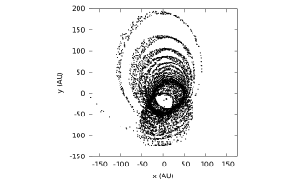
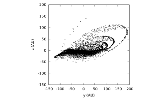
In Fig. 3 we give the distribution of the KB as obtained by model A. The figure presents the projection of the sampled system onto the and the planes yr after the closest approach between the Sun and the perturbing star. Some KBOs were scattered out to a heliocentric distances exceeding 200 , and with very high eccentricities, but the majority () of objects remains bound. Moreover the KBOs are distributed in over densities triggered by the passing of the star which are resonances due to the planets contribution.
In Figs. 4 and 5 we show the distributions for eccentricity and inclination as a function of the semi-major axis for the KBOs from model A. Here we varied the impact parameter parameters and inclination of the encounter. The mass of the passing-by star was 1 M⊙ for these simulations and the total mass of the KB was M⊕. These simulations were performed with KBOs and run up to yr.
In the Figures we have identified three main regimes, which we colored red, green and blue, indicating the highly, intermediate and relatively little perturbed system, respectively.
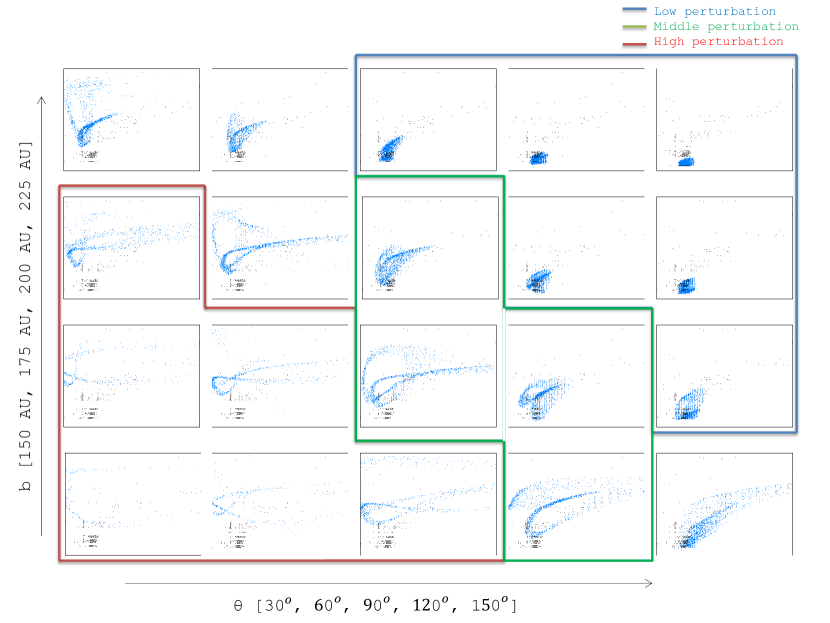
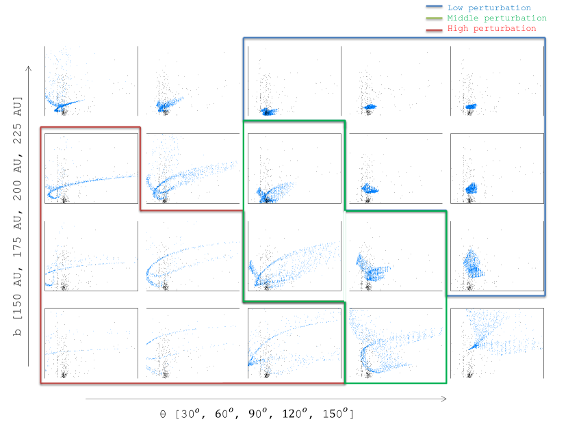
In the highly perturbing encounter (red zone in figs. 4 and 5) the KB is almost completely destroyed. In the moderately perturbing encounter (blue zone) the post-encounter KBO is characterized by that the majority of objects remain confined in the classical region but with slightly elevated eccentricities and inclinations. These distributions are most comparable to the observed eccentricities and inclinations in the classic (observed) regions. However, the resonance regions and the scattered region are notoriously depleted compared to the observations. In particular, the distribution in inclinations is too much concentrated around a mean value, whereas the observed inclinations are distributed more evenly between to .
The distribution of eccentricities in the mildly perturbed encounters (green zone in figs. 4 and 5) has almost vanished and some objects have scattered to very small semi-major axes. The general shape of the KBO, however, seems to follow the data more closely that those that result from the other more strongly perturbed interactions. The majority of bodies resides in the classical part of the KB with an extended tail of monotonically increasing eccentricities with the semi-major axis, indicating an almost constant periastron distance. On the down-side, however, the distribution of inclinations is distinctively different than the observations.
We compare the distributions in eccentricities and inclinations of the KBOs at yr after the encounter changing the total mass of the KB with values and M⊕ and the sampling of the KBOs with in range [8182, 131,062] fixing the and parameters. This comparison is performed using the two-dimensional Kolmogorv-Smirnov tests (Press et al., 2002). The tests give probabilities for eccentricity as well as inclination . The K-S test is a measure of the difference in the two distributions. The high values of these K-S test is an indication that the distributions, obtained varying the principal parameters of the sampling of the KB, show very small differences. Therefore, a small variation of the initial conditions for the KB gives rise to only small changes in final distribution, and on the short time frame of the encounter, the effect of the passing star is considerably stronger than any internal dynamical effect inside the KB. The effect the passing star has on the KB is almost impulsive, and variations in the mass of the passing star strongly affects the eccentricities and inclinations of the KBOs. These distributions therefore provide a sensitive characterization to constrain the mass and orbital parameters of the incoming star.
It may be relevant noting that some of the consequences of the encounter of star with the KB can be reliably predicted by the much simpler test particle approach, i.e. neglecting the internal interactions between the KBOs. Actually, a comparison of our results with test-particle simulations (Ida et al., 2000; Kobayashi & Ida, 2001; Kobayashi et al., 2005; Melita et al., 2005) show a certain level of similarities:
-
1.
a stellar encounter pumps up strongly the eccentricities and inclinations of objects in the outer region of a planetesimal disk. Moreover, if the classical KBOs acquire high eccentricities their perihelia migrate to the inside.
-
2.
a strong stellar encounter (corresponding to star passing close to the KB disk) may deplete the original, flat, KBO distribution up to 95. However, contrary to Kobayashi et al. (2005), we find that a strong depletion correspond to a full destruction of the Solar system structure. On the other hand, we found also reasonable initial encounter conditions leading to “intermediate” cases, where a significant depletion (at about level) is compatible with the observed distributions of eccentricities and inclinations.
-
3.
it is not possible to populate the observed resonances reproducing exactly the overdensity in the eccentricity and inclination distributions invoking only a fly-by star perturbation (see Ida et al. (2000)).
The strong effect of the incoming star is clearly depicted in Figs. 4 and 5. Varying the mass of the encountering star cases a migration in both and . The low-mass star (0.5 M⊙) gives rise to a shift to smaller values of and , whereas a higher mass star (2 M⊙) causes a shift toward larger values of both parameters.
The early evolution of the system strongly depends on the initial conditions of the passing star. We therefore decided to run more simulations in the middle regime (green zone) in the range and , and in a the second regime of and . All the simulations show a characteristic tail to a monotonically increasing eccentricities; quite similar to the distribution of the eccentricities of the observed scattered KBOs. This tail is characteristic for the relatively close encounter with a stellar perturber, and we confirm the earlier made conjecture of such an encounter (Ida et al., 2000). The distribution in inclination, however, is still to easily reproduced.
To validate our visual comparison we performed a statistical cross-comparison between the observational and computational data for each of the simulations in Tab. 1 using the Hotelling’s two sample test (Hotelling, 1931), which is a generalization of the Student’s test, where
| (3) |
with the Fisher-Snededecor random variable and is defined as:
| (4) |
where is the pooled sample covariance matrix of and , namely,
| (5) |
where is the covariance matrix of the sample for , is the mean of the sample, and the sample for each random variable in has elements, and similarly is the covariance matrix of the sample for , is the mean of the sample, and the sample for each random variable in has elements. The Hotelling’s test states that two population are indistinguishable if
| (6) |
where is the number of parameters, the significance level of the test and is the theoretical value of -distribution. In Tab. 2 we present the values for . Each -value is the comparison between two samples: the observed KBOs and the computational one. In order to calculate the variable we compute it using the JD2000 Ephemeris (Right Ascension and Declination coordinates) of the observed KBOs and on the coordinates of the computational KBOs converted in equatorial coordinates. We have normalized the values with (where is our number of KBOs parameter and is the number of observed KBOs (Marsden, 1980)). In the table (Tab. 2) we have subtracted one from the result to make the clearer distinction that negative values represent results for which the computational and the observational distributions are statistically indistinguishable. We did not perform the Hotelling’s test directly on the eccentricity and inclination distributions because the test can be calculated only on two samples that have a normal distributions. On the other hand, (,) are not independent from (,) values, therefore a negative value in Tab. 2 tells also information about the eccentricity and inclination distributions.
This test suggests that encounters with a large impact parameter or large inclination are favored (strictly speaking, the other runs are rejected on this statistical). Although this method does not makes a distinction in quality of the results, other than accepting or rejecting it, the area of parameter space that give small perturbations (blue zone) seems to be favored. These simulations show a cold and low-eccentricity population of KBOs.
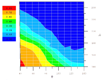
In Fig. 6 we present the fraction of KBOs that escaped the Solar System as a result of the stellar encounter. Based on these results we prefer the highly scattered regime, with a low value for and (red zone). In fact only in the highly perturbed regime there is a substantial loss of mass which can reconcile the difference of two magnitude between the total mass observed and the total mass predicted by Solar System formation models (Luu & Jewitt, 2002).
These contradicting results let us to perform a second series of simulations in which we adopted a wider range of semi-major axis, this we called model B.
| 30 | 60 | 70 | 80 | 90 | 100 | 110 | 120 | 150 | |
|---|---|---|---|---|---|---|---|---|---|
| 225 | -0.1 | -0.7 | - | - | -0.8 | - | - | -0.9 | -0.8 |
| 200 | 7.0 | 1.3 | 0.8 | 0.2 | 0.0 | - | - | -0.7 | -0.6 |
| 190 | - | - | 1.6 | 0.9 | 0.1 | - | - | - | - |
| 180 | - | - | 2.0 | 1.3 | 0.8 | - | - | - | - |
| 175 | 4.7 | 2.3 | 1.3 | 0.3 | 0.4 | - | - | -0.6 | 0.0 |
| 170 | - | - | - | - | 0.5 | 0.7 | -0.4 | - | - |
| 160 | - | - | - | - | -0.5 | 0.1 | -0.2 | - | - |
| 150 | 2.3 | 1.1 | - | - | -0.1 | 0.1 | -0.1 | -0.3 | 0.1 |
| 140 | - | - | - | - | -0.5 | 0.0 | 0.5 | - | - |
3.2 Model B
In model B we adopted a wider radial extension of the KBO, 42 to 90 with a total mass of M⊕. The mass and encounter parameters of the incoming star are presented in Tab. 1. The success of model A in reproducing the observed parameters for the KBO led us to limit our parameter search this more extended distribution to and . The results of the Hotelling test are presented in Tab. 3.
| 60 | 75 | 90 | 105 | 120 | 135 | 150 | |
|---|---|---|---|---|---|---|---|
| 237.5 | -0.6 | -0.8 | -0.8 | -0.9 | -0.8 | -0.4 | -0.7 |
| 225 | -0.2 | -0.8 | -0.6 | -0.7 | -0.9 | -0.2 | -0.7 |
| 212.5 | -0.3 | -0.5 | -0.7 | -0.7 | -0.8 | -0.9 | -0.4 |
| 200 | 0.1 | -0.3 | -0.7 | -0.8 | -0.5 | -0.9 | -0.4 |
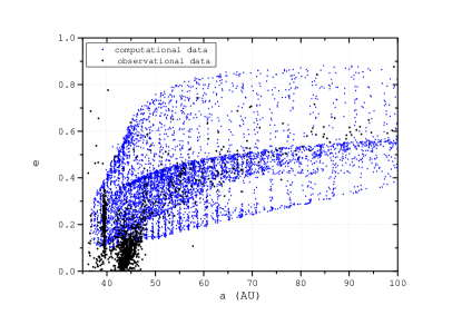
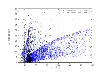
In Fig. 7 we present the distributions for eccentricity and inclination for and . We determine it as the best model which gives a much better match with the observed inclinations; with value ranging from roughly up to in the classical regime and up to in the scattered regime whereas the eccentricities of the scattered population and the high-eccentricity population in the classical region are consistent with the observational data. With these parameters the initial KB lost of its mass in the encounter, which is quite small compared to the predictions (Luu & Jewitt, 2002).
The parameters for this particular encounter has trouble reproducing the low-eccentricity population; in fact, the minimum value of the eccentricities in the classical regime . For this reason we started a series of simulations in which we study the long-term secular evolution of the KB, on which we report in § 3.3.
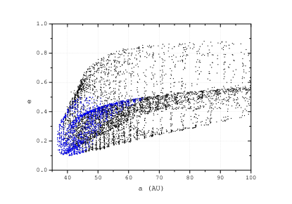
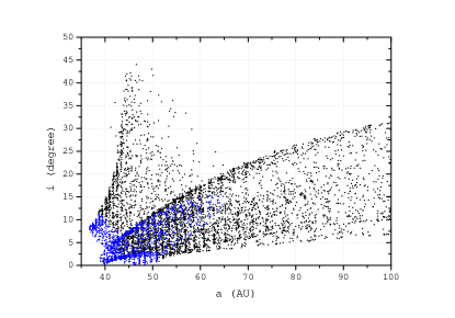
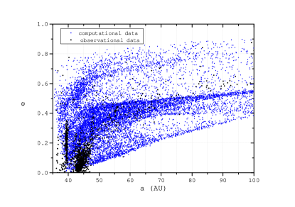
For comparison we highlighted, in Fig. 8 the eccentricities after the encounter for model A and model B for one particular encounter. For the range where the initial conditions of model A and B overlap, the post-encounter distributions in eccentricity and inclination also overlap. This supports the earlier argument that inter-KBO dynamics is not important during the encounter.
3.3 Long term evolution
The main result for model A and B has been that an encounter in the early history of the Solar System can reproduce the high-eccentricity KB population as well as the majority of the scattered population, but the currently observed low-eccentricity population and part of the resonant populations are absent after the encounter. We will now investigate if these missing populations can be regrown by the long-term evolution of the KB.
We adopt model A with a 1 encountering star with an impact parameter and inclination for this follow-up study. Ideally, we should have taken the best model B, but because the missing populations are reachable with the limited range in semi-major axes in model A, we decided that the benefit of the higher local resolution of this model outweighs the more extended width of model B. We restart the simulation at yr after the encounter. For convenience we removed the encountering star, because it would cause numerical problems if we allowed it to continue to move further away from the Solar System, whereas it would no longer perturb the KB.
a) 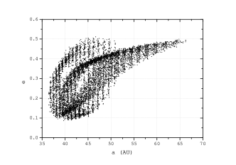
b) 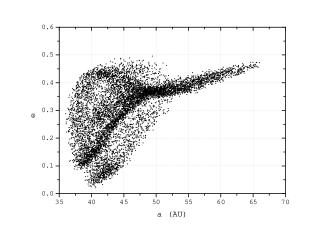
c) 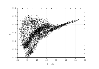
d) 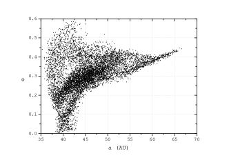
In Fig. 9 we present the evolution of the eccentricities and semi-major at four moments in time. This illustrates the effect of the secular evolution of the KBOs, due to their self gravity and the influence of the planets. Whereas the encounter with the star completely removes the low-eccentricity population, the subsequent long-term evolution within the KB regrows this population. During the secular evolution the high eccentricity orbits contained between and “cool” to lower eccentricities. In this model we considered KBOs () with a total mass of 30 M⊕; each KBO, then, has the mass M⊕.
An important test of the importance of mutual gravitational interactions between KBOs in determining the KB secular evolution has been done through the expedient of “switching off” the pair interaction. We saw that these simulations did not show the “cooling” of the KB populations, with eccentricities which remained too high compared to the observations. We were driven to conclude that the mutual interactions among the KBOs are responsible of the secular evolution to the partial repopulation of the low-eccentricity distribution after a stellar encounter.
In Tab. 4 we present a summary of results of several simulations at varying and the KBO radius, which correspond to a variation of the individual KBO mass. Initial conditions are those of model A. We noted that, as expected, the time needed to repopulate the low-eccentricity KBO distribution ( in the right most column of Tab. 4) scales roughly as the two body relaxation time scale, which, in a virialized system, has the following dependence on and (Binney & Tremaine, 1987):
| (7) |
| label | M | (km) | (Myr) | |
|---|---|---|---|---|
| 1 | 1741 | 0.50 | ||
| 2 | 808 | 1.58 | ||
| 3 | 375 | 5.00 | ||
| 4 | 1741 | 0.77 | ||
| 5 | 1741 | 1.15 | ||
| 6 | 808 | 3.64 | ||
| 7 | 100 | 91.56 |
After establishing the initial conditions which we considered to produce the observed KB, we run one more simulations, with and a total mass of 30 M⊕ (35% of the KBOs have a mass identical to Pluto, while the others have only one-fifth of this mass). The incoming 1 star has approaches the Sun with impact parameter and inclination . We continue this simulation for 0.9 Myr.
In Fig. 10 we present the energy conservation and the total number of escapers in function of time. The distribution of the eccentricities at 0.9 Myr after the encounter is shown in Fig.11.

4 Conclusions
We investigated the effect of an encounter between a passing star on the morphology of the Kuiper belt, and its subsequent long-term evolution. Using the current morphology of the KB we constrained the parameter of the incoming star. The orbit of the encountering star, the planets and those of the KBOs were integrated directly, as was the subsequent evolution of the internal dynamics of the KB and planets. The initial conditions for the Solar System ware taken from Ito & Tanikawa (2002), and the Kuiper belt objects were distributed in a flat disk between 42 and 90 in the plane of the Ecliptic, and with a power law density distribution with exponent . The total mass of Kuiper belt ranged between 1 and 30 M⊕, and the mass of the incoming star was chosen to be 0.5 1.0 and 2.0 .
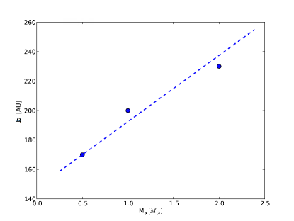
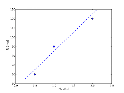
We compared the morphology of the KB directly after the encounter with the passing star, and after a secular evolution of up to 0.9 Myr. The best results, directly after the encounter, are obtained when the incoming star approached the ecliptic plane with an impact parameter of 170-220 and an inclination above the Ecliptic of to . The lower (best) values of both and are for the 0.5 , encountering star whereas the upper values correspond to the 2.0 intruder. We summarize these results in Tab. 5. In Fig. 12 we present the impact parameter and the angle of the incoming star as a function of its mass. A correlation between these parameters is evident and shows a degeneration in the parameters space. In fact, using different parameters is possible to reproduce an encounter with the same strength and find similar proprieties in the final KBOs distributions.
During this encounter about 13% of the Kuiper belt is lost from the Solar system. Actually, results do not show a depletion of the original flat distribution up to as suggested by the observed total mass of the KB, evaluated in the range M⊕, and the mass estimation from Solar system formation model, M⊕, (Luu & Jewitt, 2002) and match the eccentricity and inclination distributions with the observation at the same time. On the other hand, a better coverage of the initial conditions of the incoming star can very likely enhance the possibility of finding an intermediate case, where a strong depletion can be compatible with the observed distributions in eccentricities and inclinations.
The morphology of the high-eccentricity and scattered population of the KB are well represented directly after the encounter. The low-eccentricity population, around and with eccentricities is almost completely absent directly after the encounter. This mismatch in the morphology can be resolved by taking the secular evolution of the Kuiper belt into account. The low-eccentricity population is reinstated within a million years. Our models did not show any particular correlation between the inclinations distributions and the mass of the KBOs. However, due to the limited number of objects in our simulations, we could run only almost single-mass particle simulations. For example in our best model the gap in mass between the two population is only a factor 5 and the ratio between the radius is 1.7. Due to this limitation it is not possible to constrain any significant correlations among inclination and other properties, such as the size distribution of the KBOs and the number of KBO binaries. In conclusion, the sampling limiting our model and the relatively short time-scale of our simulations cannot give reliable results on that (actually, our finest simulation involved 16384 KBOs and was carried up to 0.9 Myear).
We expect that a more sophisticated investigation of the long-term (Myr) evolution of the KB, with a proper population over the whole KBO mass spectrum will show the “relaxation” of the eccentricities to low values as it happens in the case of mass monodisperse-particle simulations. Such detailed studies would thus provide important information about the final distribution of the KBOs, which will allow a complete comparison with observable such as the size-inclination relation, but unfortunately it is hard to achieve at the moment without the access to a very large GPUs cluster.
While the secular evolution repopulated the low-eccentricity population, it triggered the further KB causing the depletion of the resonance population, which was initiated by the passing star. This loss of the resonant population can be due to the insufficient sampling of the KB in our simulations. Alternatively, the early migration of the planets is driving the repopulation of the resonant families (Malhotra, 1995; Ida et al., 2000). Such planetary reordering would be a natural consequence of the Nice model (Levison et al., 2008). Moreover, the resonances, that we have suddenly after the passage of the fly-by star, do not show an eccentricity and inclination distributions compatible with the observations.
| M | 0.5 | 1.0 | 2.0 |
|---|---|---|---|
5 Acknowledgments
D. Punzo thanks the Leiden Observatory (University of Leiden) for a period of hospitality. This work was made possible also thanks to a financial contributions from the Dept. of Physics (Sapienza, University of Rome), from the Netherlands Research Council NWO (grants #643.200.503, #639.073.803 and #614.061.608), from the Netherlands Research School for Astronomy (NOVA), and from the HPC-EUROPA2 project (project number: 1249) with the support of the European Commission - Capacities Area - Research Infrastructures. Most of the computations were carried out on the computers owned by the ASTRO research group (Dep. of Physics, Sapienza, Univ. of Roma) and on the Little Green Machine at Leiden University and on the Lisa cluster at SURFSara in Amsterdam and by. We finally thank M. Spera for his help in porting the code to various architectures.
References
- Aarseth (2003) Aarseth S. J., 2003, Gravitational N-Body Simulations
- Bédorf & Portegies Zwart (2012) Bédorf J., Portegies Zwart S., 2012, European Physical Journal Special Topics, 210, 201
- Berczik et al. (2011) Berczik P., Nitadori K., Zhong S., Spurzem R., Hamada T., Wang X., Berentzen I., Veles A., Ge W., 2011, in International conference on High Performance Computing, Kyiv, Ukraine, October 8-10, 2011., p. 8-18 High performance massively parallel direct N-body simulations on large GPU clusters.. pp 8–18
- Berczik et al. (2013) Berczik P., Spurzem R., Wang L., 2013, in Third International Conference ”High Performance Computing”, HPC-UA 2013, p. 52-59 Up to 700k GPU cores, Kepler, and the Exascale future for simulations of star clusters around black holes.. pp 52–59
- Bernstein et al. (2004) Bernstein G. M., Trilling D. E., Allen R. L., Brown M. E., Holman M., Malhotra R., 2004, Astronomical Journal, 128, 1364
- Binney & Tremaine (1987) Binney J., Tremaine S., 1987, Galactic dynamics
- Brown (2001) Brown M. E., 2001, Astronomical Journal, 121, 2804
- Brucker et al. (2009) Brucker M. J., Grundy W. M., Stansberry J. A., Spencer J. R., Sheppard S. S., Chiang E. I., Buie M. W., 2009, Icarus, 201, 284
- Capuzzo-Dolcetta et al. (2011) Capuzzo-Dolcetta R., Mastrobuono-Battisti A., Maschietti D., 2011, New Astronomy, 16, 284
- Capuzzo-Dolcetta & Spera (2013) Capuzzo-Dolcetta R., Spera M., 2013, Computer Physics Communications, 184, 2528
- Capuzzo-Dolcetta et al. (2013) Capuzzo-Dolcetta R., Spera M., Punzo D., 2013, Journal of Computational Physics, 236, 580
- Doressoundiram et al. (2008) Doressoundiram A., Boehnhardt H., Tegler S. C., Trujillo C., 2008, Color Properties and Trends of the Transneptunian Objects. pp 91–104
- Fraser & Kavelaars (2009) Fraser W. C., Kavelaars J. J., 2009, Astronomical Journal, 137, 72
- Gomes (2003) Gomes R. S., 2003, Icarus, 161, 404
- Holman (1995) Holman M. J., 1995, in Kinoshita H., Nakai H., eds, 27th Symposium on Celestial Mechanics, The Distribution of Mass in the Kuiper Belt. p. 116
- Hotelling (1931) Hotelling H., 1931, Annals of Mathematical Statistics, 2, 360
- Ida et al. (2000) Ida S., Larwood J., Burkert A., 2000, The Astrophysical Journal, 528, 351
- Ito & Tanikawa (2002) Ito T., Tanikawa K., 2002, Monthly Notices of the Royal Astronomical Society, 336, 483
- Jewitt & Luu (1993) Jewitt D., Luu J., 1993, Nature, 362, 730
- Kenyon & Luu (1999) Kenyon S. J., Luu J. X., 1999, Astronomical Journal, 118, 1101
- Kobayashi & Ida (2001) Kobayashi H., Ida S., 2001, Icarus, 153, 416
- Kobayashi et al. (2005) Kobayashi H., Ida S., Tanaka H., 2005, Icarus, 177, 246
- Levison et al. (2008) Levison H. F., Morbidelli A., Van Laerhoven C., Gomes R., Tsiganis K., 2008, Icarus, 196, 258
- Levison & Stern (2001) Levison H. F., Stern S. A., 2001, Astronomical Journal, 121, 1730
- Luu & Jewitt (2002) Luu J. X., Jewitt D. C., 2002, Astronomy and Astrophysics, 40, 63
- Malhotra (1993) Malhotra R., 1993, Nature, 365, 819
- Malhotra (1995) Malhotra R., 1995, Astronomical Journal, 110, 420
- Malmberg et al. (2011) Malmberg D., Davies M. B., Heggie D. C., 2011, Monthly Notices of the Royal Astronomical Society, 411, 859
- Marsden (1980) Marsden B. G., 1980, Celestial Mechanics, 22, 63
- Melita et al. (2005) Melita M. D., Larwood J. D., Williams I. P., 2005, Icarus, 173, 559
- Nitadori & Makino (2008) Nitadori K., Makino J., 2008, New Astronomy, 13, 498
- Noll et al. (2008) Noll K. S., Grundy W. M., Stephens D. C., Levison H. F., Kern S. D., 2008, Icarus, 194, 758
- Nyland et al. (2007) Nyland L., Harris M., Prins J., , 2007, Fast N-Body Simulation with CUDA
- Pelupessy et al. (2012) Pelupessy F. I., Jänes J., Portegies Zwart S., 2012, New Astronomy, 17, 711
- Pelupessy et al. (2013) Pelupessy F. I., van Elteren A., de Vries N., McMillan S. L. W., Drost N., Portegies Zwart S. F., 2013, Astronomy and Astrophysics, 557, A84
- Portegies Zwart & Boekholt (2014) Portegies Zwart S., Boekholt T., 2014, ArXiv e-prints
- Portegies Zwart et al. (2009) Portegies Zwart S., McMillan S., Harfst S., Groen D., Fujii M., Nualláin B. Ó., Glebbeek E., Heggie D., Lombardi J., Hut P., Angelou V., Banerjee S., Belkus H., Fragos T., Fregeau J., Gaburov E., Izzard R., 2009, New Astronomy, 14, 369
- Portegies Zwart et al. (2013) Portegies Zwart S., McMillan S. L. W., van Elteren E., Pelupessy I., de Vries N., 2013, Computer Physics Communications, 183, 456
- Portegies Zwart (2009) Portegies Zwart S. F., 2009, The Astrophysical Journal, 696, L13
- Portegies Zwart et al. (2007) Portegies Zwart S. F., Belleman R. G., Geldof P. M., 2007, New Astronomy, 12, 641
- Press et al. (2002) Press W. H., Teukolsky S. A., Vetterling W. T., Flannery B. P., 2002, Numerical recipes in C++ : the art of scientific computing
- Volk & Malhotra (2011) Volk K., Malhotra R., 2011, The Astrophysical Journal, 736, 11