ABSTRACT

Metastable excited states ${}^{3}P_{2},{}^{3}P_{0}$ of heavy alkaline earth atoms of even isotopes are studied for parity violating (PV) effects in radiative emission of neutrino pair (RENP). PV terms arise from interference between two diagrams containing neutrino pair emission of valence spin current and nuclear electroweak charge density proportional to the number of neutrons in nucleus. This mechanism gives large PV effects, since it does not suffer from the suppression of 1/(electron mass) usually present for non-relativistic atomic electrons. A controllable magnetic field is crucial to identify RENP process by measuring PV observables. Results of PV asymmetries under the magnetic field reversal and the photon circular polarization reversal are presented for an example of Yb atom.

Key words

Neutrino mass, Parity violation, Majorana particle, Beyond the standard gauge theory

I Introduction

For an unambiguous test of the weak nature of interaction it is crucial to directly observe odd quantities under parity operation. Parity violation in atomic transitions has been one of the key steps towards verification of the neutral current structure in electron interaction with nucleus. Mixture of different parity states in heavy atoms [1] is caused by Z-boson exchange interaction with nucleus and its existence has been verified in atomic parity violation experiments [2], [3], [4].

A hint of new physics beyond the standard gauge theory of $SU(3)\times SU(2)\times U(2)$ has been found in neutrino oscillation experiments, establishing finite neutrino masses with mixing. The first stage of oscillation experiments has been able to determine two mass squared differences and three mixing angles [5]. The next important steps are to determine (1) the mass difference pattern, the normal vs inverted mass hierarchical pattern, (2) the absolute neutrino mass scale or the smallest neutrino mass, and (3) determination of the nature of mass terms, Majorana or Dirac mass, along with their CP properties. Besides the oscillation experiments nuclear targets are main tools of ongoing experiments [6], [7].

We proposed a new method towards a future neutrino physics; the use of atoms. Parity violation is important to the new proposed process of macro-coherent radiative emission of neutrino pair (RENP), $|e\rangle\rightarrow|g\rangle+\gamma+\nu\nu$ from metastable atomic state $|e\rangle$ [8], [9], to demonstrate that the weak interaction is involved, thereby establishing experimental identification of RENP under a possible presence of QED backgrounds. We advanced a step forward towards this direction, and studied PV effects in alkaline earth atoms of odd isotopes [10]. Alkaline earth atoms are excellent for the purpose of PV effects, since two low lying metastable states of ${}^{3}P_{2},{}^{3}P_{0}$ for the initial RENP $|e\rangle$ state have different parity from the ground $|g\rangle$ state, which is required for PV effects. PV arises from interference between parity odd (PO) and parity even (PE) amplitudes. In the scheme of [10] hyperfine interaction with nucleus of odd isotopes has been used in the PE amplitude. In the present work we shall examine alkaline earth atoms of even isotopes where hyperfine interaction is absent.

We rely on an external magnetic field for even isotopes to mix $J=2,0$ state with $J=1$ state necessary for PE amplitude of intermediate transition ${}^{3}P_{2,0}\rightarrow{}^{\pm}P_{1}\rightarrow{}^{1}S_{0}$ (${}^{\pm}P_{1}$ is the mixture of ${}^{3}P_{1}$ and ${}^{1}P_{1}$ caused by spin-orbit interaction). The mixing amplitude by the magnetic field is of order $\mu_{B}B\sim 50\mu{\rm eV}B/{\rm Tesla}$ divided by energy difference of levels, to be compared with hyperfine mixing of $O(\mu{\rm eV})$ [10]. The advantage of the external magnetic field in alkaline earth atoms of even isotopes has been demonstrated in another context, the clock transition of Yb atom [11]. It turns out that the required Coulomb interaction with nucleus for RENP PE amplitude gives rise to a large amplitude in accordance with discussion in [12]. Thus, the magnetic field application may also be important to achieve a large enhancement for alkaline earth atoms of odd isotopes, but we shall discuss only even isotopes in order to avoid unnecessary complications of the mechanism. Another merit of the applied magnetic field in even isotopes is its controllability of magnitudes and direction in measurement of PV observables. It should thus help much in identification of RENP process in experiments.

In a series of theoretical papers we developed and gradually refined a new, systematic experimental method to probe the neutrino mass matrix using RENP. Following the initial idea [8], we first discussed how to enhance otherwise small neutrino pair emission rates [13], [9], and then how to extract neutrino parameters from the photon energy spectrum [14], [9]. In the most recent work we pointed out how to obtain a much larger RENP rate [12] using a coherent neutrino pair emission from nucleus where the zero-th component of vector current operates much like the enhanced admixture of different parity states in atomic PV experiments. Our experimental efforts towards RENP are briefly described in [9]. Clearly, investigation of PV effects is the next important step in RENP.

The rest of this work is organized as follows. In Section II how PV observables may arise in the standard electroweak theory (with finite neutrino masses) by listing all PO and PE pair emission vertexes to the leading and the next sub-leading orders of 1/mass. Some technical details on the phase space integral of neutrino pair variables (helcities and momenta) that have a direct relevance to emergence of parity odd quantities are relegated to Appendix A. We then calculate in Section III amplitudes of RENP, emphasizing how the magnetic field dependence is disentangled. In Section IV RENP rates, both parity conserving (PC) and PV, are calculated. PC rates and PV asymmetries are given in analytic forms using explicitly known elementary functions: dependences on parameters of the neutrino mass matrix elements are thereby clearly worked out. We then illustrate results of numerical computations on PV observables and its asymmetry under the magnetic field and the photon circular polarization reversals, taking the example of the Yb $J=2\rightarrow 0$ transition. (PV effects are found to vanish for ${}^{3}P_{0}$.) The rates have an overall uncertain factor subject to detailed numerical simulations dependent on experimental conditions. The spectral shape is however determined unambiguously as function of neutrino parameters. We are able to present spectral shapes and PV asymmetries assuming a single unknown parameter of smallest neutrino mass and taking other parameters consistent with the present oscillation data [5]. Rates related to PV are insensitive to Majorana CP phases, but PV observables can measure the smallest mass, and make distinction of normal and inverted hierarchical mass pattern, and distinction of Majorana and Dirac neutrino, The rest of this work consists of summary and Appendices.

We are bound to calculate amplitudes using perturbation theory in non-relativistic quantum mechanics, hence the time ordering in higher orders of perturbation should be treated with care. This gives rise to cancellations of a few added contributions.

Throughout this work we use the natural unit of $\hbar=c=1$.

II Candidate search for parity odd and even amplitudes

Typical RENP experiments use several lasers for trigger and excitation. For instance, two continuous wave (CW) lasers of different frequencies $\omega_{i},i=1,2$ where $\omega_{1}<\omega_{2}\,,\omega_{1}+\omega_{2}=\epsilon_{eg}$ and $\epsilon_{eg}$ is the energy difference between the initial $|e\rangle$ state and the final $|g\rangle$ state, are used as triggers in counter propagating directions (taken along z-axis), while two excitation lasers of Raman type of frequencies, $\omega_{p}\,,\omega_{s}$ with $\omega_{p}-\omega_{s}=\epsilon_{eg}$ are irradiated in pulses. Measured variables at the time of excitation pulse irradiation are the number of events at each trigger frequency $\omega_{1}$. By repeating measurements at different trigger frequency combinations, one obtains the photon energy spectrum at different frequencies $\omega=\omega_{1}$ accompanying the invisible neutrino pair. If PV effects are large, measurements of PV asymmetries help reject QED backgrounds, the largest being two-photon emission.

The macro-coherent three-body RENP process $|e\rangle\rightarrow|g\rangle+\gamma+\nu\nu$ conserves both the energy and the momentum, giving continuous photon energy spectrum with thresholds. Note that the spontaneous decay of dipole transition from excited atoms conserves the energy alone, hence their spectrum is continuous despite of a single particle decay. In RENP there are six photon energy thresholds at $\omega_{ij}=\epsilon_{eg}/2-(m_{i}+m_{j})^{2}/2\epsilon_{eg}$ with $m_{ij}\,(i,j=1,2,3)$ three neutrino masses of mass eigenstates. Decomposition into six different threshold regions is made possible by excellent energy resolution of trigger laser frequencies.

PV effects arise from interference of two RENP amplitudes of parity even (PE) and parity odd (PO). Note that both rates arising from the squared PO and the squared PE amplitudes give PC rates. There are two types of neutrino pair emission amplitudes with regard to spatial behavior, $A_{0}\nu_{i}^{\dagger}\nu_{j}$, and $\vec{A}\cdot\nu_{i}^{\dagger}\vec{\sigma}\nu_{j}$, where $A_{0}$ is atomic matrix element relevant to the nuclear mono-pole current of neutrino pair emission, and $\vec{A}$ is the one relevant to the spin current from valence electron. Each of $A_{\alpha},\alpha=0,1,2,3$ contains product of E1 matrix elements, couplings and energy denominators in perturbation theory. We use two component notation for electron operators in the neutrino emission vertex of $A_{\alpha}$, following the $\gamma_{5}$-diagonal representation of [8]. Relevant leading terms for PO and PE terms for pair emission of mass eigenstates $ij$ are given by

$$A_{0}\propto e^{\dagger}\left(b_{ij}+\delta_{ij}2\sin^{2}\theta_{w}\vec{\sigma}\cdot\frac{\vec{p}}{m_{e}}+O(\frac{1}{m_{e}^{2}})\right)e+\delta_{ij}j_{q}^{0}\,,\hskip 14.22636ptj_{q}^{0}=-\frac{1}{2}j_{n}^{0}+\frac{1}{2}(1-4\sin^{2}\theta_{w})j_{p}^{0}\,,$$ (1)

$$\vec{A}\propto e^{\dagger}\left(a_{ij}\vec{\sigma}+\delta_{ij}2\sin^{2}\theta_{w}\frac{1}{m_{e}}(\vec{p}-i\vec{\sigma}\times\vec{p})+O(\frac{1}{m_{e}^{2}})\right)e\,,$$ (2)

$$a_{ij}=-U_{ei}^{*}U_{ej}+\frac{1}{2}\delta_{ij}\,,\hskip 14.22636ptb_{ij}=U_{ei}^{*}U_{ej}-\frac{1}{2}\delta_{ij}(1-4\sin^{2}\theta_{w})\,,$$ (3)

where necessary neutrino mixing matrix elements $U_{ei}$ have been determined experimentally [5] whose values we use in our following analysis. The weak mixing angle is determined experimentally; $\sin^{2}\theta_{w}\sim 0.238$. The term $j_{q}^{0}$ is the nuclear mono-pole current contribution which gives rise to coherently added constituent numbers [12]. We disregarded terms of orders of $1/m_{e}^{2}$ and $1/m_{N}$,

In order to calculate parity conserving (PC) and parity violating (PV) rates, added amplitudes are squared, and one proceeds to calculate summation over neutrino helicities and momenta, since neutrino variables are impossible to measure under usual circumstances. Thus, using formulas in [8], we find that PV parts of rates are proportional to

$$\int d{\cal P}_{\nu}\sum_{h_{k}}\Re(A_{0}\vec{A}^{*})\propto\int d{\cal P}_{\nu}\sum_{h_{k}}(\frac{\vec{p}_{i}}{E_{i}}+\frac{\vec{p}_{j}}{E_{j}})=\vec{k}\frac{J_{ij}(\omega)}{\omega}\,,$$ (4)

$$d{\cal P}_{\nu}=\frac{d^{3}p_{i}d^{3}p_{j}}{(2\pi)^{2}}\delta(\omega+E_{i}+E_{j}-\epsilon_{eg})\delta(\vec{k}+\vec{p}_{i}+\vec{p}_{j})\,.$$ (5)

The photon momentum vector $\vec{k}$ is thus multiplied to give PV operator of the form, $\vec{k}\cdot\vec{\sigma}$ where $\vec{\sigma}$ is the electron spin operator $\times 2$. The explicit form of function $J_{ij}(\omega)$ is given in eq.(54) of Appendix A.

This conclusion is consistent with the ordinary view that PV effects must arise from interference of parity odd combination of $V\cdot A$ in the product of electron and quark 4-currents. The spin current of electron $\propto\vec{\sigma}$ arises from the spatial component of 4-axial vector $A\propto\gamma^{\alpha}\gamma_{5}$ in the non-relativistic limit, while the nuclear mono-pole current $\propto j_{q}^{0}$ arises from the time component of 4-vector current $V\propto\gamma_{\alpha}$. It is the unique combination of electron and nuclear current operators that gives rise to large PV terms without the suppression of $1/$mass order, which became possible only with the advent of nuclear mono-pole contribution given in [12].

Alkaline earth atoms are two-electron system of the angular momentum combination of parity odd orbitals, $sp$. This combination of angular momenta appears as the first excited group of levels in alkaline earth atoms. Two electrons may be either in the spin triplet or the spin singlet state in the terminology of the $LS$ coupling scheme. Thus, one has four different states (with the usual magnetic degeneracy of energies), ${}^{3}\!P_{2},^{3}\!P_{1},^{3}\!P_{0},^{1}\!P_{1}$, the atomic notation of ${}^{2S+1}L_{J}$ being used [15].

Another important consideration is that it is better to use heavy (large atomic number) atoms for large RENP rates [12]. This poses a problem of state mixing in the $LS$ scheme, which requires the use of intermediate coupling scheme [16]. The $LS$ coupling scheme is based on the assumption that electrostatic interaction between electrons is much larger than the spin-orbit interaction $\sum_{i}\xi(r_{i})\vec{l}_{i}\cdot\vec{s}_{i}$, which however becomes larger for heavier atoms. In the heaviest atoms such as Pb the $jj$ coupling scheme becomes a better description [16], but most of heavy atoms is well described by the intermediate coupling scheme using the $LS$ basis.

In the intermediate coupling scheme applied to heavy alkaline earth atoms one considers the mixing among states of the same total angular momentum, since the total angular momentum is conserved under the presence of the spin-orbit interaction. These are ${}^{3}P_{1}$ and ${}^{1}P_{1}$ in the $LS$ scheme. Energy eigenstates are given in terms of the $LS$ basis [17],

$$|{}^{+}P_{1}\rangle=\cos\theta|^{1}P_{1}\rangle+\sin\theta|{}^{3}P_{1}\rangle\,,\hskip 14.22636pt|{}^{-}P_{1}\rangle=\cos\theta|{}^{3}P_{1}\rangle-\sin\theta|{}^{1}P_{1}\rangle\,,$$ (6)

(with $\pm$ denoting larger/smaller energy state) where the angle $\theta$ is determined by the strength of spin-orbit interaction in the system and is related to experimental data of level energies. In the Yb case $\sin\theta\sim 0.16$ [10]. Dipole moments $d(|{}^{\pm}P_{1}\rangle\rightarrow|{}^{1}S_{0}\rangle$ needed for RENP calculation are induced by a non-vanishing value of $\theta$.

We now turn to a concrete explanation of how PO amplitude arises, corresponding to the left diagram of Fig(1). An electron in the $ns_{1}$ level of the two-electron system of excited $ns_{1},n^{\prime}p$ state first makes a virtual transition to a vacant level in $ns_{2}$ by neutrino pair emission operator $\propto e^{\dagger}\vec{\sigma}e\cdot\nu_{i}^{\dagger}\vec{\sigma}\nu_{j}$. Another electron in the excited level $n^{\prime}p$ then fills the hole in $ns_{1}$ by a photon emission, completing the transition $|ns_{1}n^{\prime}p\rangle\rightarrow|ns_{2}ns_{1}\rangle+\gamma+\nu_{i}\nu_{j}$. One might think that another, equally contributing possibility is a process in which the neutrino pair emission and the photon emission vertexes are interchanged in the time sequence. This is the diagram in the right of Fig(1), but the quantum numbers of two-electron system changes according to ${}^{3}P_{2}\rightarrow{}^{\pm}P_{1}\rightarrow{}^{1}S_{0}$, thus this contribution is highly forbidden both by E1 and the spin operators involved.

We now turn to PE amplitude that may have a large interference with this PO amplitude. In a recent work [12] we discussed a possibility of largest PC rate using the nuclear mono-pole current (time component of 4-vector part) for neutrino pair emission. A candidate set of PE amplitude might arise from diagrams of Fig(3) and Fig(3). The neutrino pair emission $\propto Q_{w}$ occurs from the nuclear line, and the rest consists of the Coulomb interaction $\propto Z\alpha/r$ and E1 emission. The quantum numbers of atomic transition, ${}^{3}P_{2}\rightarrow{}^{\pm}P_{1}\rightarrow{}^{1}S_{0}$, dictates the time sequence of the Coulomb interaction first and E1 emission next, thus rejecting the possibility of Fig(3).

Contribution from Fig(3) is calculated as follows. Combined with the time of nuclear pair emission, there are three types of diagrams giving different energy denominators. Each of these contain numerator factors of the form,

$$\langle{}^{1}S_{0}|\vec{E}\cdot\vec{D}|{}^{\pm}P_{1}\rangle\langle{}^{\pm}P_{1}|\frac{Z\alpha}{r}|{}^{3}P_{2}\rangle=\pm\sin\theta\cos\theta\langle{}^{1}S_{0}|\vec{E}\cdot\vec{D}|{}^{1}P_{1}\rangle\langle{}^{3}P_{1}|\frac{Z\alpha}{r}|{}^{3}P_{2}\rangle\equiv\pm{\cal N}_{0}\,.$$ (7)

Amplitudes consist of six terms, considering different $|^{\pm}P_{1}\rangle$ intermediate states. Three contributions from each of $|{}^{\pm}P_{1}\rangle$, using the energy conservation $\epsilon({}^{3}P_{2})=E_{2\nu}+\omega$, add to a common factor $\pm{\cal N}_{0}$ times

$$\frac{1}{(\epsilon_{3}-\omega)(\epsilon_{\pm}-\omega)}-\frac{1}{(\epsilon_{\pm}-\epsilon_{3}\,)(\epsilon_{3}-\omega)}+\frac{1}{(\epsilon_{\pm}-\epsilon_{3}\,)(\epsilon_{\pm}-\omega)}=0\,,$$ (8)

with $\epsilon_{3}=\epsilon({}^{3}P_{2})-\epsilon({}^{1}S_{1})$. Thus, we conclude that the lowest order contribution given by Fig(3) and Fig(3) to PE amplitude vanishes and the magnetic field assistance as described in the next section is required for non-vanishing contribution.

We shall not apply external static electric field, because it may induce an instrumental parity mixture difficult to disentangle from the intrinsic parity violation of fundamental theory [18].

IV Zeeman mixing and magnetic factors

The Zeeman mixing caused by the magnetic field is described by the interaction vertex $\mu_{B}(2\vec{S}+\vec{L})\cdot\vec{B}$ [15]. This Zeeman mixing applied to our problem gives perturbed states,

$$|e\rangle^{\prime}=|e\rangle+\delta_{+e}|^{+}{}P_{1}\rangle+\delta_{-e}|^{-}{}P_{1}\rangle\,,\hskip 14.22636pt\delta_{\pm e}=\frac{\langle^{\pm}{}P_{1}|\mu_{B}(2\vec{S}+\vec{L})\cdot\vec{B}|e\rangle}{\epsilon_{\pm e}}\,.$$ (9)

The mixing amplitude $\delta_{\pm e}$, with $\mu_{B}B\sim 5.8\times 10^{-5}$eV/T, gives a small, but important transition between different $J$ states. With the Zeeman mixing inserted in diagrams of Fig(5), the product of atomic matrix elements ${\cal N}_{0}$ above is modified to

$$\pm{\cal N}\,,\hskip 14.22636pt{\cal N}=\sin\theta\cos\theta\langle{}^{1}S_{0}|\vec{E}\cdot\vec{D}|{}^{1}P_{1}\rangle\langle{}^{3}P_{1}|\mu_{B}(2\vec{S}+\vec{L})\cdot\vec{S}|{}^{3}P_{2}\rangle\langle nP|\frac{Z\alpha}{r}|nP\rangle\,.$$ (10)

The last factor $\propto Z\alpha/r$ of Coulomb energy is estimated using Thomas-Fermi model as done in [12], giving $\sim 31{\rm eV}Z^{4/3}$.

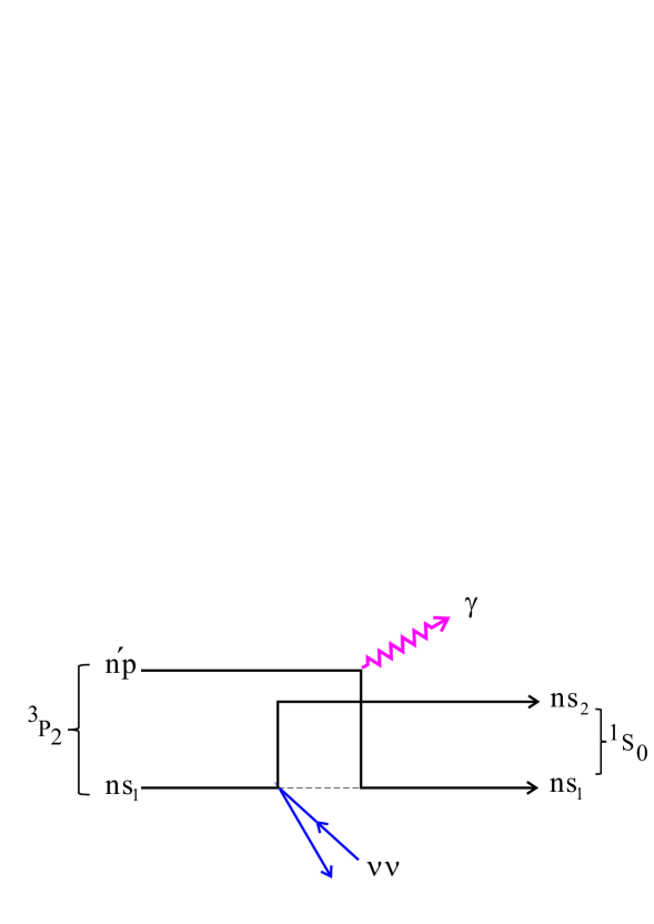
Figure 1: Parity odd contribution of valence electron exchange. Neutrino pair emission contains the PE part of vertex, as described in the text.

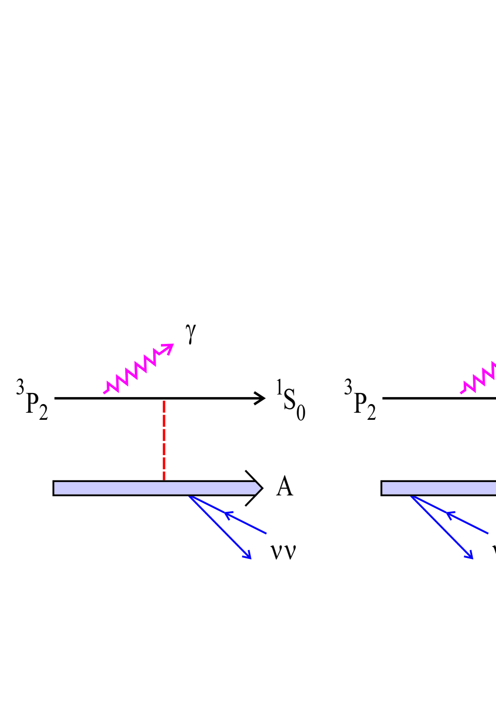
Figure 2: Rejected PE diagrams that give vanishing contribution.

 

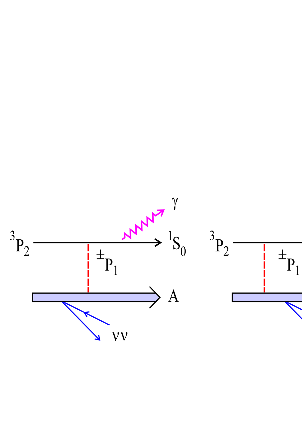
Figure 3: Candidate PE diagrams.

We now turn to detailed description of this unique candidate for PV effect. There are five vertexes to be considered and we shall treat these basic interaction units as shown in Fig (4) on an equal footing. Five types of interactions have to be considered; valence transition by Zeeman field $\mu_{B}(2S+L)\cdot B$ of Fig (4) (a), E1 photon emission $d\cdot E$ (b), neutrino pair emission from valence electron which leads to parity violation (c), neutrino pair emission from nucleus (by the mono-pole current as described in [12]) (d), and Coulomb interaction between valence electron and nucleus $V_{C}$ (e).

Five units of interaction along the valence electron line are given by five vertex matrix elements of operators,

$$\mu_{B}(2\vec{S}+\vec{L})\cdot\vec{B}\,,\hskip 8.5359pt\vec{d}\cdot\vec{E}\,,\hskip 8.5359pta_{ij}\vec{\sigma}_{e}\nu_{i}^{\dagger}\vec{\sigma}\nu_{j}\,,\hskip 8.5359ptQ_{w}\nu_{i}^{\dagger}\nu_{j}\,,\;(Q_{w}\equiv N-0.044Z)\,,\hskip 8.5359pt\frac{Z\alpha}{r}\,.$$ (11)

RENP amplitudes consist of factors of these basic units, energy denominators in perturbation theory, and coupling factors. Neutrino pair emission gives rise to product of two plane wave functions of definite helicities. For Majorana pair emission the wave function of two neutrinos must be anti-symmetrized, since Marjorana particles are identical to their own anti-particles and effects of identical fermions work, to give rise to the principle of Majorana-Dirac distinction [8].

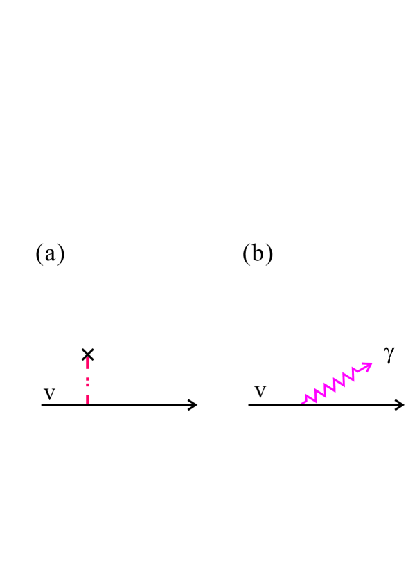
Figure 4: Five basic units of interaction. Cross is for Zeeman field, dotted line for instantaneous Coulomb interaction. v means the valence electron line and A is atomic nucleus.

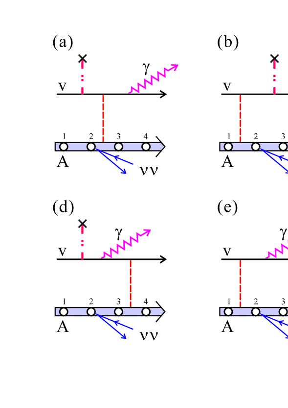
Figure 5: 24 PC RENP diagrams. Along the nuclear line neutrino pair emission may occur in four places in time sequence relative to three vertexes along the valence line, four different nuclear vertex locations giving different amplitudes. In our 3-level approximation only (a) and (c) contribute.

It is important, and experimentally useful, to work out effects of magnetic field directional dependence. This magnetic field dependence of amplitudes and rates is called the magnetic factor generically in the following. We consider the experimental setup in which a static magnetic field is applied in a general direction tilted by an angle $\theta_{m}$ from the trigger z-axis (which is also the direction of emitted photon). Magnetic quantum numbers $M$ of states are defined as components of $\vec{J}$ along the quantization axis, namely the magnetic field direction. To emphasize directionality we denote states by the notation of tilde, hence

$$\widetilde{|J,M\rangle}=e^{-i\theta_{m}J_{y}}|J,M\rangle=\sum_{M^{\prime}}d^{J}_{M,M^{\prime}}(\theta_{m})|J,M^{\prime}\rangle\,,$$ (12)

where $d^{J}_{M,M^{\prime}}(\theta_{m})$ is the Wigner d-function or the rotation matrix in the terminology of [20].

Let us first work out the magnetic factor associated with the PE (parity even) amplitude. The magnetic factor for emission of the photon circular polarization $h=\pm$ is given by

$$\sum_{M}\langle{}^{1}S_{0}|erY_{1,\pm 1}\widetilde{|{}^{\pm}P_{1}M\rangle}\langle{}^{\pm}P_{1}\tilde{M}|(2\tilde{S}+\tilde{L})_{z}\widetilde{|{}^{3}P_{2}M^{\prime}\rangle}\,,$$ (13)

$$\sum_{M}\langle{}^{1}S_{0}|erY_{1,\pm 1}\widetilde{|{}^{\pm}P_{1}M\rangle}\widetilde{\langle{}^{\pm}P_{1}M|}(2\tilde{S}+\tilde{L})_{z}\widetilde{|{}^{3}P_{0}M^{\prime}\rangle}\,.$$ (14)

The operator $erY_{1,\pm}$ is the atomic dipole transition operator for emission of the specified photon circular polarization $h=\pm$. Since summation over magnetic quantum numbers in intermediate states can be taken along any axis, we took the axis along the magnetic field, which makes calculations easier. (The magnetic quantum number in the initial state is taken along with the magnetic field, which is dictated in the experimental setup.)

The magnetic field mixes states of ${}^{3}P_{2,0}$ and ${}^{\pm}P_{1}$ by the atomic operator $2\vec{S}+\vec{L}=\vec{J}+\vec{S}$. The total angular momentum $\vec{J}$ here does not contribute since $\Delta J\neq 0$ in two involved states. This implies that only ${}^{3}P_{1}$ components of ${}^{\pm}P_{1}$ have non-vanishing matrix element of

$$\widetilde{\langle{}^{3}P_{1},M_{J}|}(2\tilde{\vec{S}}+\tilde{\vec{L}})_{q}\widetilde{|{}^{3}P_{2}\rangle}\langle{}^{3}P_{1},M_{J}|(2\vec{S}+\vec{L})_{q}|{}^{3}P_{2}\rangle=\sqrt{\frac{5}{2}}(-1)^{1-M_{J}}\left(\begin{array}[]{ccc}1&1&2\\ -M_{J}&q&M_{J}-q\end{array}\right)$$ (17)

A similar relation exists for the transition from ${}^{3}P_{0}$. Reduced matrix element, $\langle{}^{3}P_{1}||\vec{S}||{}^{3}P_{2}\rangle=\sqrt{5/2}$ was used. Thus, the magnetic factor associated with PE amplitude is given by

$$\sum_{M}\langle{}^{1}S_{0}|Y_{1,\pm 1}\widetilde{|{}^{\pm}P_{1}M\rangle}\langle{}^{\pm}P_{1}\tilde{M}|(2\tilde{S}+\tilde{L})_{z}\widetilde{|{}^{3}P_{2}M^{\prime}\rangle}$$

$$=\pm\sqrt{\frac{5}{2}}\langle{}^{1}S_{0}|er|{}^{1}P_{1}\rangle\sin\theta\cos\theta d^{1}_{M^{\prime},\mp 1}(-1)^{1-M^{\prime}}\left(\begin{array}[]{ccc}1&1&2\\ -M^{\prime}&0&M^{\prime}\end{array}\right)\,,$$ (20)

$$\sum_{M}\langle{}^{1}S_{0}|Y_{1,\pm 1}\widetilde{|{}^{\pm}P_{1}M\rangle}\widetilde{\langle{}^{\pm}P_{1}M|}(2\tilde{S}+\tilde{L})_{z}\widetilde{|{}^{3}P_{0}M^{\prime}\rangle}$$

$$=\pm\sqrt{\frac{5}{2}}\langle{}^{1}S_{0}|er|{}^{1}P_{1}\rangle\sin\theta\cos\theta d^{1}_{M^{\prime},\mp 1}(-1)^{1-M^{\prime}}\delta_{M^{\prime},0}\left(\begin{array}[]{ccc}1&1&0\\ 0&0&0\end{array}\right)\,.$$ (23)

We may define the magnetic factors for amplitudes by extracting out dipole matrix element $\langle{}^{1}S_{0}|er|{}^{1}P_{1}\rangle\sin\theta\cos\theta$, which is related to measured A-coefficient and energy difference of atomic levels, The magnetic factor for ${}^{3}P_{2}$ is

$$W_{1,\pm}^{M}(x)=\sqrt{\frac{5}{2}}(-1)^{1-M}\left(\begin{array}[]{ccc}1&1&2\\ -M&0&M\end{array}\right)d^{1}_{M,\mp 1}(x)\,.$$ (26)

Similar magnetic factor for PO amplitude is defined by taking into account of the neutrino phase space integration which gives $\vec{k}$, the wave vector of emitted photon. It is for ${}^{3}P_{2}$ RENP

$$\sum_{M}\langle{}^{1}S_{0}|Y_{1,\pm 1}\widetilde{|{}^{\pm}P_{1}M\rangle}\widetilde{\langle{}^{\pm}P_{1}M}|(2S+L)_{z}\widetilde{|{}^{3}P_{2}M^{\prime}\rangle}\,.$$ (27)

Note that the definite field direction along the trigger axis (fixed as parallel to $z$ axis) is selected, hence no tilde operation in this formula of angular momenta. Thus, the magnetic factor for PO is more complicated;

$$W_{2,\pm}^{M}(x)=-\sqrt{\frac{5}{2}}\sum_{M_{1},M_{2}}(-1)^{1-M_{1}}\left(\begin{array}[]{ccc}1&1&2\\ -M_{1}&0&M_{1}\end{array}\right)d^{2}_{M,M_{1}}(x)d^{1}_{M_{2},M_{1}}(x)d^{1}_{M_{2},\pm 1}(x)\,.$$ (30)

Explicit forms of these functions are given in Appendix B. They are simple linear combinations of sinusoidal functions.

PV odd rates are given by differences of the product of magnetic factors for PO and PE amplitudes. It turns out that the PO product magnetic factor for ${}^{3}P_{0}$ RENP vanishes, and we shall work out quantities for ${}^{3}P_{2}$ RENP in the following. There are two kinds of PV asymmetries one can calculate from these magnetic factors: the first one is PV asymmetry under the magnetic field reversal, $x\rightarrow\pi-x$, and the other is the asymmetry under the reversal of the photon circular polarization, $h=\pm\rightarrow\mp$, for which all angle dependences may be integrated out. PV asymmetry under field reversal is dictated by the magnetic factor,

$${\cal M}^{M}(x)\equiv\sum_{\pm}{\cal M}^{M}_{\pm}(x)\,,\hskip 14.22636pt{\cal M}^{M}_{\pm}(x)=W_{1,\pm}^{M}(x)W_{2,\pm}^{M}(x)-W_{1,\pm}^{M}(\pi-x)W_{2,\pm}^{M}(\pi-x)\,.$$ (31)

Explicitly worked out, these are

$${\cal M}^{\pm 1}(x)=-\frac{1}{2}\cos^{3}x\,,\hskip 14.22636pt{\cal M}^{0}(x)=\sin^{2}x\cos x\,.$$ (32)

Non-vanishing values at various angles may be taken as indication of parity violation in RENP. The simplest PV asymmetry of this kind is the forward-backward asymmetry given by ${\cal M}_{1}^{0}(0)=0$ and ${\cal M}_{1}^{\pm}(0)=-\frac{1}{2}$. For normalized asymmetries rate differences should be divided by PE combinations of angular factors,

$${\cal M}_{1}^{M}(x)\equiv\sum_{\pm}(W_{1,\pm}^{M}(x)\,)^{2}+(W_{1,\pm}^{M}(\pi-x)\,)^{2}\,,$$ (33)

$${\cal M}_{2}^{M}(x)\equiv\sum_{\pm}W_{1,\pm}^{M}(x)W_{2,\pm}^{M}(x)+W_{1,\pm}^{M}(\pi-x)W_{2,\pm}^{M}(\pi-x)\,.$$ (34)

Explicit forms of these are listed in Appendix B.

The other PV asymmetry under the reversal of the photon circular polarization is given by

$$\int_{-\pi}^{\pi}dx\left({\cal M}_{+}^{\pm 1}(x)-{\cal M}_{-}^{\pm 1}(x)\right)=\pm 0.39\,,\hskip 14.22636pt\int_{-\pi}^{\pi}dx\left({\cal M}_{+}^{0}(x)-{\cal M}_{-}^{0}(x)\right)=0\,.$$ (35)

These magnetic factors are plotted for magnetic quantum numbers of $M=\pm 1,0$ in Fig(6). Directional dependence of PV asymmetries is large and should help much in proving the weak origin of RENP process.

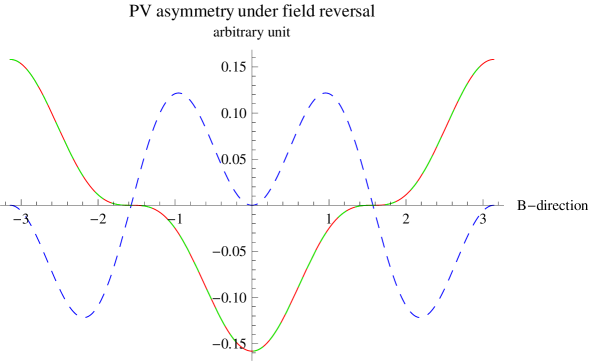
Figure 6: ${}^{3}P_{2}\rightarrow^{1}\!S_{0}$ PV asymmetry under field reversal for the sum of two circular polarizations vs B-direction measured from the trigger axis. Initial magnetic quantum number of $M=\pm 1$ (the degenerate case) is depicted in solid red and dash-dotted green, and $M=0$ in dashed blue.

V PV interference, PC rate and PV asymmetry

RENP spectral rates may be expressed by two formulas $\Gamma_{2\nu\gamma}^{\pm}(\omega)$ which are interchanged by reversal of instrumental polarity; the magnetic field direction and the direction of circular polarizations. Rates may be written as

$$\Gamma_{2\nu\gamma}^{\pm}(\omega)=\Gamma_{2\nu\gamma}^{PC1}(\omega)+\Gamma_{2\nu\gamma}^{PC2}(\omega)\pm\Gamma_{2\nu\gamma}^{PV}(\omega)\,.$$ (36)

The last term is the interference term arising from the product of PE and PO amplitudes, while the first two terms result from the squared PE and PO amplitudes. We decompose these three spectral rates, both parity conserving (PC) and parity violating (PV), into an overall factor denoted by $\Gamma_{0}$, various spectral shape functions of kinematical nature, atomic factors, and the dynamical factor $\eta_{\omega}(t)$. We shall use a unit of 100 MHz for A-coefficients (decay rates) and eV for all energies. We give rates appropriate for Yb $J=2\rightarrow 0$ RENP. The conversion factor in our natural unit is $\hbar c=1.97\times 10^{-5}{\rm eV}\cdot{\rm cm}$.

The overall rate is given by

$$\Gamma_{0}=\frac{3}{4}G_{F}^{2}\epsilon_{eg}n^{3}V\frac{\gamma_{+g}}{\epsilon_{+g}^{3}}(\sin\theta\cos\theta)^{2}\eta_{\omega}(t)$$ (37)

$$\sim 54{\rm mHz}(\frac{n}{10^{21}{\rm cm}^{-3}})^{3}\frac{V}{10^{2}{\rm cm}^{3}}\frac{\epsilon_{eg}}{{\rm eV}}\frac{\gamma_{pg}{\rm eV}^{3}}{\epsilon_{pg}^{3}{\rm 100MHz}}(\sin\theta\cos\theta)^{2}\eta_{\omega}(t)\,.$$ (38)

The factor $\sin\theta\cos\theta$ reflects the strength of the spin-orbit interaction in heavy atoms. As representative values of atomic data we may take the dominant dipole strength $d_{pg}=\sqrt{3\pi\gamma_{pg}/\epsilon_{pg}^{3}}$, of state $|p\rangle=^{+}\!P_{1}$ for Yb. Electric field strength of emitted photons has been written as $|E|^{2}=\epsilon_{eg}n\eta_{\omega}(t)$ where $\epsilon_{eg}n$ is the maximum stored energy density stored in the upper level $|e\rangle$. Thus, one may regard $\eta_{\omega}(t)$ as the fraction of extractable energy density within the target. This quantity may be computed numerically using the PSR master equation [9].

Individual contributions are given as follows. We present results for PV asymmetry under field reversal using ${\cal M}_{i}=\sum_{M}{\cal M}_{i}^{M}(\theta_{m})$ for the magnetic factor. For the asymmetry under polarization reversal this function should be replaced by the integrated quantity (35).

(1) PC rate from squared PE amplitudes is given by

$$\Gamma_{2\nu\gamma}^{PC1}=\Gamma_{0}Q_{w}^{2}V_{C}^{2}\left(\sum_{p=\pm}\epsilon_{pe}\delta_{pe}F_{C}(\omega;\epsilon_{p})\right)^{2}I(\omega){\cal M}_{1}(\theta_{m})\,,\hskip 14.22636ptI(\omega)=\sum_{i}I_{ii}(\omega)\theta(\omega_{ii}-\omega)\,,$$ (39)

$$I_{ii}(\omega)=\frac{1}{2}(\,C_{ii}(\omega)+A_{ii}(\omega)+\delta_{M}m_{1}m_{2}D_{ii}(\omega)\,)\,,\hskip 14.22636ptV_{C}\sim 31{\rm eV}Z^{4/3}\,,\hskip 14.22636ptQ_{w}=N-0.044Z\,,$$ (40)

$$F_{C}(\omega;\epsilon_{p})=\frac{1}{(\epsilon_{eg}-\omega)(\epsilon_{pg}-\omega)^{2}}+\frac{1}{\epsilon_{pe}(\epsilon_{pg}-\omega)^{2}}+\frac{1}{\epsilon_{pe}^{2}(\epsilon_{pg}-\omega)}+\frac{1}{\epsilon_{pe}^{2}(\epsilon_{pe}+\omega)}\,.$$ (41)

We refer to Appendix A for all spectral shape functions here and in the follwoing,
$A_{ii}(\omega)\,,B_{ii}(\omega)\,,C_{ii}(\omega)\,,D_{ii}(\omega)\,,J_{ii}(\omega)$ that arise from the neutrino phase space integration.

(2) PC rate arising from squared valence PO amplitude is

$$\Gamma_{2\nu\gamma}^{PC2}=\Gamma_{0}f_{vc}^{2}H(\omega;\theta_{m}){\cal M}_{2}(\theta_{m})\,,\hskip 14.22636ptH(\omega;\theta_{m})=\sum_{i}a_{ii}^{2}H_{ii}(\omega)\theta(\omega_{ii}-\omega)\,,$$ (42)

$$H_{ii}(\omega)=\frac{1}{2}\left(C_{ii}(\omega)-A_{ii}(\omega)-\delta_{M}m_{i}^{2}D_{ii}(\omega)\right)+\frac{B_{ii}(\omega)}{\omega^{2}}\,,\hskip 14.22636ptf_{v}(\omega)=-\frac{1}{\epsilon_{+g}-\omega}-\frac{\gamma_{-g}\epsilon_{+g}^{3}}{\gamma_{+g}\epsilon_{-g}^{3}}\frac{1}{\epsilon_{-g}-\omega}\,.$$ (43)

(3) Interference term between PO and PE amplitudes is given by

$$\Gamma_{2\nu\gamma}^{PV}=\Gamma_{0}Q_{w}f_{v}(\omega)V_{C}\left(\sum_{p=\pm}\epsilon_{pe}\delta_{pe}F_{C}(\omega;\epsilon_{p})\right)J(\omega){\cal M}(\theta_{m})\,,$$ (44)

$$J(\omega)=\sum_{i}a_{ii}J_{ii}(\omega)\theta(\omega_{ii}-\omega)\,,\hskip 14.22636ptJ_{ii}(\omega)=-\frac{\Delta_{ii}(\omega)}{4\pi}\omega\left(\epsilon_{eg}-\frac{4}{3}\omega+\frac{4(\epsilon_{eg}-\omega)m_{i}^{2}}{3\epsilon_{eg}(\epsilon_{eg}-2\omega)}\right)\,.$$ (45)

Note that three different magnetic factors, ${\cal M}\,,{\cal M}_{1,2}$, appear in three terms.

PV asymmetry is defined by

$${\cal A}(\omega)=\frac{2\Gamma_{2\nu\gamma}^{PV}}{\Gamma_{2\nu\gamma}^{PC1}+\Gamma_{2\nu\gamma}^{PC2}}\,.$$ (46)

This is a quantity to be compared with the experimental asymmetry obtained by taking the ratio of the difference to the sum of two rates when reversal of experimental setup variables is made to change instrumental parity. The PV asymmetry ${\cal A}(\omega)$ of eq.(46) is a function of $M$ (the initial magnetic quantum number of ${}^{3}P_{2}$ state) and $h$ the circular polarization.

VI Numerical calculation of RENP spectral rates

A-coefficients we need for computations of ${}^{174}_{70}$Yb RENP are $\gamma_{+g}=176,\gamma_{-g}=1.1$MHz’s and $\epsilon_{+g}=3.108,\epsilon_{-g}=2.2307,\epsilon(^{3}P_{2})=2.4438$eV’s. The contribution of intermediates state ${}^{+}P_{1}$ dominates over ${}^{-}P_{1}$ with these parameters due to larger values of $d^{2}=3\pi\gamma/\epsilon^{3}$; $\gamma_{-g}\epsilon_{+g}^{3}/(\gamma_{+g}\epsilon_{-g}^{3})\sim 0.017$ for Yb. $\sin\theta\cos\theta\sim 0.158$ has been estimated for Yb [10]. The dominant Zeeman mixing is given by $\delta_{+e}$ with energy difference $\epsilon_{+e}\sim 0.664$ eV. Hence the magnetic mixing $\delta_{+e}=5\times 10^{-6}$ corresponds to a magnetic field strength $\sim 57$ mT. The nuclear electroweak is taken for even isotope ¹⁷⁴Yb, giving $Q_{w}\sim 101$.

It is convenient to define a quantity which may be called figure of merits; the product of squared asymmetry times PC rates. This measures a statistical significance of asymmetry measurements. The figure of merits is plotted against the magnetic mixing $\delta\sim 5\times 10^{-5}$Tesla/eV, in Fig(8). The magnitude of PV asymmetry under the reversal of circular polarization is shown in Fig(8). These results indicate that there is an optimal choice of the magnetic field strength, implying that a largest field strength is not necessarily the best choice. Based on this result we shall choose for the following figures an optimal Zeeman mixing of $\sim 5\times 10^{-6}$ which gives an optimal magnetic field strength $\sim 60$ mT.

In Fig(9) $\sim$ Fig(11) we illustrate results of calculation for RENP PV spectrum differences and PV asymmetry, assuming the smallest neutrino mass of 5 meV in which other neutrino parameters are taken consistently with existing oscillation data. In these and other figures a target number density $n=10^{22}$cm^-3 and the target volume $V=10^{2}$cm³ and the dynamical factor $\eta_{\omega}(t)=1$ are taken, rates scaling with $n^{3}V\eta_{\omega}(t)$. Except in Fig(10) where two different PV asymmetries are compared, all other diagrams exhibit PV asymmetry under the reversal of photon circular polarization. Distinction of the normal hierarchical (NH) and the inverted hierarchical (IH) mass patterns is easier for PV than PC as seen in Fig(9). Overall PV rates for an optimal magnetic field are typically of order $10^{3}$ larger than hyperfine mixing in alkaline earth atoms of odd isotopes given in [10].

Dependence on the magnetic quantum number $M$ of $J=2$ levels are as follows. The magnitudes of PV asymmetries for $M=\pm 1$ are the same, while they vanish for $M=\pm 2,0$.

Distinction of Majorana and Dirac neutrinos is of great interest. Parity violating asymmetries do distinguish these two cases when measurements by appropriate choice of magnetic field $\approx$100 mT are made in the low photon energies as evident in Fig(10) even for a smallest neutrino mass of 5 meV.

Fig(12) shows dependence of PV asymmetry shapes on the magnetic field strength for a few choices of measured photon energies, which clearly indicates the importance of the field magnitude in actual experiments.

Although parity violation effects do not exist for ${}^{3}P_{0}$ Yb RENP, it is of interest to compare its PC rates with ${}^{3}P_{2}$ case. This is shown in Fig(13). In both cases NH and IH differences are small, and difficult to resolve their differences in this figure.

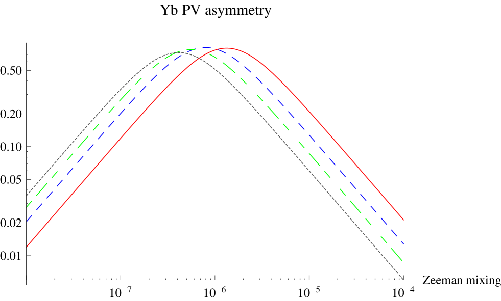
Figure 7: Yb PV asymmetry under the reversal of photon circular polarization plotted against the Zeeman mixing parameter $\delta_{+g}$, assuming a single neutrino of mass 50 meV, the target number density $10^{22}$cm^-3, and the target volume $10^{2}$cm³. Assumed photon energies are the level spacing of Yb 2.44 eV $\times$ 0.1 in solid red, 0.2 in dashed blue, 0.3 in dash-dotted green, and 0.4 in dotted black.

 

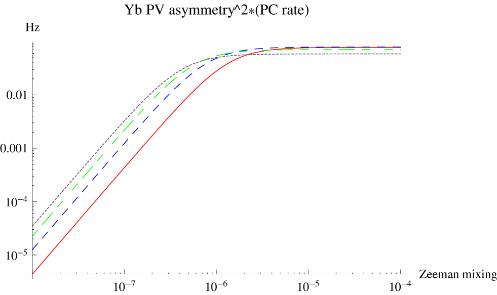
Figure 8: Yb PV asymmetry squared $\times$ PC rate (figure of merits) plotted against the Zeeman mixing parameter $\delta_{+g}$, corresponding to Fig(8).

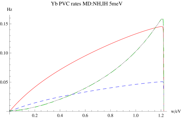
Figure 9: ${}^{3}P_{2},J=2,M_{J}=1$ Yb PC rates, PV rate differences. Zeeman mixing amplitude $5\times 10^{-6}$ (corresponding to the magnetic field $\sim 60$ mT), $\eta_{\omega}(t)=1$, $n=10^{22}$cm^-3, and $10^{2}$cm³ are assumed. Majorana NH PV in solid red, M-IH PV in dashed blue, M-NH PC rate divided by 50 in dash-dotted green, and M-IH/50 in dotted black (degenerate with M-NH PC).

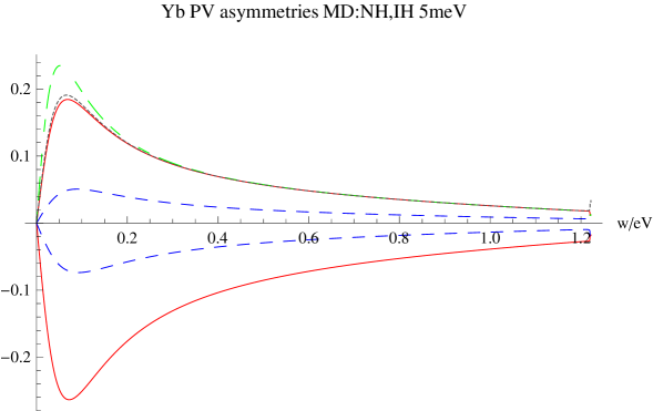
Figure 10: ${}^{3}P_{2}$Yb PV asymmetries vs photon energy. Zeeman mixing amplitude $5\times 10^{-6}$, $\eta_{\omega}(t)=1$, $n=10^{22}$cm^-3, and $10^{2}$cm³ assumed. In the positive side the Majorana case of PV asymmetry under polarization reversal for NH is depicted in solid red, M-IH case in dashed blue, D-NH in dash-dotted green and the Dirac case for NH in dotted black. In the negative side PV asymmetry under the field reversal is plotted; M-NH in solid red, and M-IH in dashed blue, all assuming the smallest neutrino mass 5 meV.

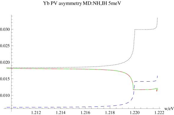
Figure 11: ${}^{3}P_{2},J=2,M_{J}=1$ Yb PV asymmetry in the threshold regions corresponding to Fig(10).

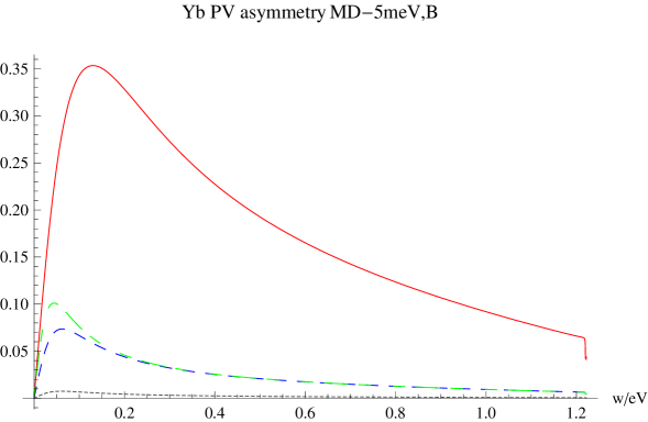
Figure 12: ${}^{3}P_{2},J=2,M_{J}=1$ Yb PV asymmetries under the reversal of photon circular polarization for a few choices of magnetic fields, $B=10$mT in solid red, $100$mT in dashed blue, $1$T in dotted black, in the case of Majorana NH, and the Dirac NH case of $100$mT in dot-dashed green. The assumed smallest neutrino mass is 5 meV.

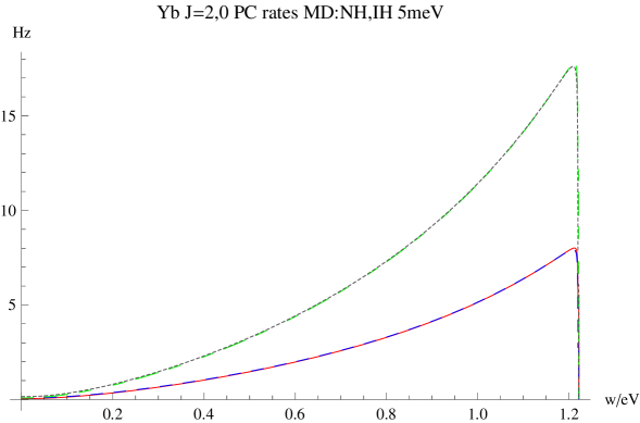
Figure 13: Comparison of rates from ${}^{3}P_{2},J=2,M_{J}=1$ and ${}^{3}P_{0}$ Yb PC rates, $\eta_{\omega}(t)=1$, $n=10^{22}$cm^-3, and $10^{2}$cm³ are assumed. Majorana NH PC rate from ${}^{3}P_{2}$ in solid red, M-IH PC in dashed blue, while Majorana NH PC rate from ${}^{3}P_{0}$ in dot-dashed green and in dotted black.

Finally, we note that our method of computation is readily applicable to other alkaline-earth-like atoms, including an electron-hole system such as Xe excited states of $6s6p$ having the same quantum numbers ${}^{3}P_{2}$.

VII Summary

We examined how parity violating asymmetry and PV rate difference in RENP may be observed in atomic de-excitation. Our proposed mechanism uses interference terms of parity even and odd amplitudes that do not suffer from the usual atomic velocity suppression $v/c$, since we use for the neutrino pair emission the spin current contribution from the valence electron and the nuclear mono-pole contribution from nucleus. Large PV interference and PV asymmetry may occur in transitions among different parity states, which suggests alkaline earth atoms as good targets. Necessary state mixing between different $J$ states occurs by an external magnetic field for alkaline earth atoms of even isotopes. Fundamental formulas applicable when magnetic sub-levels are energetically resolved are derived and used for numerical computations. The PV asymmetry may readily reach of order several tenths of unity in the examined case of Yb. Spectral shapes and PV asymmetries are sensitive to the smallest neutrino mass, difference of the hierarchical mass patterns, the Majorana-Dirac distinction. Sensitivity to the applied magnetic field strength may greatly help identification of RENP process. A further systematic search for better target atoms of number density close to the Avogadro number per cm³, in particular ions implanted in transparent crystals, is indispensable for realistic RENP experiments along with extensive numerical simulations of the time dependent dynamical factor ($\eta_{\omega}(t)$).

VIII Appendices

Appendix A: Neutrino phase space integral

Using the helicity summation formula of [8] and disregarding irrelevant T-odd terms, one has

$$\hskip 28.45274pt\sum_{h_{i}}|j_{0}^{\nu}\cdot A_{0}+\vec{j}^{\nu}\cdot\vec{A}|^{2}=$$

$$\frac{1}{2}(1+\frac{\vec{p}_{1}\cdot\vec{p}_{2}}{E_{1}E_{2}}+\delta_{M}\frac{m_{1}m_{2}}{E_{1}E_{2}})|A_{0}|^{2}+\frac{1}{2}(1-\frac{\vec{p}_{1}\cdot\vec{p}_{2}}{E_{1}E_{2}}-\delta_{M}\frac{m_{1}m_{2}}{E_{1}E_{2}})|\vec{A}|^{2}+\frac{\Re(\vec{p}_{1}\cdot\vec{A}\vec{p}_{2}\cdot\vec{A}^{*})}{E_{1}E_{2}}-2(\frac{\vec{p}_{1}}{E_{1}}+\frac{\vec{p}_{2}}{E_{2}})\Re(A_{0}\vec{A}^{*})\,,$$

(47)

where $(E_{i},\vec{p}_{i})$ are neutrino 4-momenta. In the phase space integral of neutrino momenta,

$$\int d{\cal P}_{\nu}(\cdots)=\int\frac{d^{3}p_{1}d^{3}p_{2}}{(2\pi)^{2}}\delta(E_{1}+E_{2}+\omega-\epsilon_{eg})\delta(\vec{p}_{1}+\vec{p}_{2}+\vec{k})(\cdots)$$ (48)

one of the momentum integration is used to eliminate the delta function of the momentum conservation. The resulting energy-conservation is used to fix the relative angle factor $\cos\theta$ between the photon and the remaining neutrino momenta, $\vec{p}_{1}\cdot\vec{k}=p_{1}\omega\cos\theta$. Noting the Jacobian factor $E_{2}/p\omega$ from the variable change to the cosine angle, one obtains one dimensional integral over the neutrino energy $E_{1}$:

$$\frac{1}{2\pi\omega}\int_{E_{-}}^{E_{+}}dE_{1}E_{1}E_{2}\frac{1}{2}(\cdots)\,,\hskip 14.22636ptE_{2}=\epsilon_{eg}-\omega-E_{1}\,.$$ (49)

The angle factor constraint $|\cos\theta|\leq 1$ places a constraint on the range of neutrino energy integration,

$$E_{\pm}=\frac{1}{2}\left((\epsilon_{eg}-\omega)(1+\frac{m_{i}^{2}-m_{j}^{2}}{\epsilon_{eg}(\epsilon_{eg}-2\omega)})\pm\omega\Delta_{ij}(\omega)\right)\,,$$ (50)

$$\Delta_{ij}(\omega)=\left\{\left(1-\frac{(m_{i}+m_{j})^{2}}{\epsilon_{eg}(\epsilon_{eg}-2\omega)}\right)\left(1-\frac{(m_{i}-m_{j})^{2}}{\epsilon_{eg}(\epsilon_{eg}-2\omega)}\right)\right\}^{1/2}\,.$$ (51)

We record for completeness all four important integrals over the neutrino pair momenta:

$$\int d{\cal P}_{\nu}\frac{1}{E_{1}E_{2}}=\frac{\Delta_{12}(\omega)}{2\pi}\equiv D_{12}(\omega)\,,$$ (52)

$$\int d{\cal P}_{\nu}1=\frac{\Delta_{12}(\omega)}{2\pi}\left(\frac{1}{4}(\epsilon_{eg}-\omega)^{2}-\frac{\omega^{2}}{12}+\frac{\omega^{2}(m_{1}^{2}+m_{2}^{2})}{6\epsilon_{eg}(\epsilon_{eg}-2\omega)}-\frac{\omega^{2}(m_{1}^{2}-m_{2}^{2})^{2}}{12\epsilon_{eg}^{2}(\epsilon_{eg}-2\omega)^{2}}-\frac{(\epsilon_{eg}-\omega)^{2}(m_{1}^{2}-m_{2}^{2})^{2}}{2\epsilon_{eg}^{2}(\epsilon_{eg}-2\omega)^{2}}\right)\equiv C_{12}(\omega)\,,$$

(53)

$$\int d{\cal P}_{\nu}(\frac{\vec{p}_{1}}{E_{1}}+\frac{\vec{p}_{2}}{E_{2}})=-\frac{\Delta_{12}(\omega)}{4\pi}\vec{k}\left(\epsilon_{eg}-\frac{4}{3}\omega+\frac{2(\epsilon_{eg}-\omega)(m_{1}^{2}+m_{2}^{2})}{3\epsilon_{eg}(\epsilon_{eg}-2\omega)}-\frac{4}{3}\frac{(\epsilon_{eg}-\omega)(m_{1}^{2}-m_{2}^{2})^{2}}{\epsilon_{eg}^{2}(\epsilon_{eg}-2\omega)^{2}}\right)\equiv\vec{k}\frac{J_{12}(\omega)}{\omega}\,,$$ (54)

$$\int d{\cal P}_{\nu}\frac{p_{1}^{i}p_{2}^{j}+p_{1}^{j}p_{2}^{i}}{2E_{1}E_{2}}=\frac{1}{2}(\delta_{ij}-\frac{k^{i}k^{j}}{\omega^{2}})A_{12}(\omega)+\frac{1}{2\omega^{2}}(3\frac{k^{i}k^{j}}{\omega^{2}}-\delta_{ij})B_{12}(\omega)\,,$$ (55)

$$A_{12}(\omega)=\int d{\cal P}_{\nu}\frac{\vec{p}_{1}\cdot\vec{p}_{2}}{E_{1}E_{2}}$$

$$=\frac{\Delta_{12}(\omega)}{2\pi}\left(-\frac{1}{4}(\epsilon_{eg}-\omega)^{2}+\frac{5}{12}\omega^{2}+\frac{1}{2}(m_{1}^{2}+m_{2}^{2})+\frac{\omega^{2}(m_{1}^{2}+m_{2}^{2})}{6\epsilon_{eg}(\epsilon_{eg}-2\omega)}-\frac{1}{12}\frac{(m_{1}^{2}-m_{2}^{2})^{2}}{\epsilon_{eg}^{2}(\epsilon_{eg}-2\omega)^{2}}(\omega^{2}+3(\epsilon_{eg}-\omega)^{2}\,)\right)\,,$$ (56)

$$B_{12}(\omega)=\int d{\cal P}_{\nu}\frac{\vec{k}\cdot\vec{p}_{1}\vec{k}\cdot\vec{p}_{2}}{E_{1}E_{2}}=-\frac{\Delta_{12}(\omega)}{2\pi}\frac{\omega^{2}}{12}(\epsilon_{eg}^{2}-2\omega\epsilon_{eg}-2\omega^{2})\,.$$ (57)

Appendix B: Magnetic factors

It is important to clarify the magnetic field dependence of PV observables, since this should help much to identify RENP events in actual experiments. In two types of diagrams of Fig(1) and Fig(5) the magnetic field dependence is in atomic matrix elements of the form,

$$N_{PO,\pm}^{M}=\sum_{M_{J}}\langle^{1}S_{0}|Y_{1,\pm 1}\widetilde{|^{1}P_{1},M_{J}\rangle}\widetilde{\langle^{3}P_{1},M_{J}|}S_{z}\widetilde{|^{3}P_{2},M\rangle}\,,$$ (58)

$$N_{PE,\pm}^{M}=\sum_{M_{J}}\langle^{1}S_{0}|Y_{1,\pm 1}\widetilde{|^{1}P_{1},M_{J}\rangle}\widetilde{\langle^{3}P_{1},M_{J}|}\tilde{S}_{z}\widetilde{|^{3}P_{2},M\rangle}\,,$$ (59)

where $\widetilde{|J,M\rangle}=e^{-i\theta_{m}J_{y}}|J,M\rangle$ is the rotated state of a magnetic state, as described in the text. We need these functions for two circularly polarized trigger of $\pm 1$ for E1 emission as distinguished by the spherical harmonics $Y_{1,\pm 1}$. Difference in two cases is in the spin component, either along the fixed trigger axis in the PO case or along the magnetic field in the PE case.

PE case is easier to work out, since

$$\widetilde{\langle^{3}P_{1},M_{J}|}\tilde{S}_{z}\tilde{|^{3}P_{2},M\rangle}=\langle^{3}P_{1},M_{J}|S_{z}|^{3}P_{2},M\rangle\,.$$ (60)

The result is given using 3j symbols,

$$N_{PE,\pm}^{M}(x)=-\sqrt{\frac{5}{2}}(-1)^{1-M}\left(\begin{array}[]{ccc}1&1&2\\ -M&0&M\end{array}\right)d^{1}_{M,\mp 1}(x)\,.$$ (63)

More explicitly,

$$N_{PE,\pm}^{\mp 1}(x)=\frac{1}{12\sqrt{2}}(1\pm\cos x)\,,\hskip 14.22636ptN_{PE,0}^{\pm 1}(x)=\pm\frac{1}{6\sqrt{3}}\sin x\,.$$ (64)

This gives $-W_{1,\pm}^{M}(x)$ in the text.

On the other hand, PO magnetic factors are written in terms of the product of three Wigner d-functions, and the final result is summarized by

$$N_{\pm 1,z}^{M}=-\sqrt{\frac{5}{2}}\sum_{|M_{J},M_{1}|\leq 1}(-1)^{1-M_{1}}\left(\begin{array}[]{ccc}1&1&2\\ -M_{1}&0&M_{1}\end{array}\right)d^{1}_{M_{J},\mp 1}d^{1}_{M_{J},M_{1}}d^{2}_{M,M_{1}}=-\frac{1}{18}\sqrt{\frac{5}{2}}W_{2,\pm}^{M}\,.$$ (67)

The final function is the one in the text. Explicit forms are worked out:

$$W_{2,\mp}^{\pm}=\frac{1}{4}(\cos x+\cos(2x)\,)\,,\hskip 14.22636ptW_{2,\pm}^{\pm}=\frac{1}{4}(\cos x-\cos(2x)\,)\,,\hskip 14.22636ptW_{2,0}^{\pm}=\pm\frac{1}{4}\sqrt{\frac{3}{2}}\sin(2x)\,.$$ (68)

On the other hand, magnetic factors of PE amplitudes are given by $(W_{1,\pm}^{M})^{2}$ for PE and $W_{1,\pm}^{M}W_{2,\pm}^{M}$ for PO. Their explicit forms are

$${\rm PE\;squared\;amplitudes};\;(Mh)=(1,1),(-1,-1);\hskip 8.5359pt\frac{1}{10}\cos^{4}\frac{x}{2}\,,$$ (69)

$$\hskip 14.22636pt(Mh)=(1,-1),(-1,1);\hskip 8.5359pt\frac{1}{10}\sin^{4}\frac{x}{2}\,,$$ (70)

$$\hskip 14.22636pt(Mh)=(0,\pm 1);\hskip 8.5359pt\frac{1}{15}\sin^{2}x$$ (71)

$${\rm PO\;squared\;amplitudes};\;(Mh)=(1,1),(-1,-1);\hskip 8.5359pt\frac{1}{4}\sin^{4}\frac{x}{2}(1+2\cos x)^{2}\,,$$ (72)

$$\hskip 14.22636pt(Mh)=(1,-1),(-1,1);\hskip 8.5359pt\frac{1}{4}\cos^{4}\frac{x}{2}(1-2\cos x)^{2}$$ (73)

$$\hskip 14.22636pt(Mh)=(0,\pm 1);\hskip 8.5359pt\frac{3}{32}\sin^{2}(2x)\,.$$ (74)

Multiplying PO and PE amplitudes, one obtains PV observables. The magnetic factor for PV observable thus derived is given by

$${\rm PV\;observables};\;(Mh)=(1,1),(-1,-1);\hskip 8.5359pt\frac{1}{2\sqrt{10}}\cos^{4}\frac{x}{2}(1-2\cos x)\,,$$ (75)

$$\hskip 14.22636pt(Mh)=(1,-1),(-1,1);\hskip 8.5359pt-\frac{1}{2\sqrt{10}}\sin^{4}\frac{x}{2}(1+2\cos x)\,,$$ (76)

$$\hskip 14.22636pt(Mh)=(0,\pm 1);\hskip 8.5359pt\frac{1}{2\sqrt{10}}\cos x\sin^{2}x\,.$$ (77)

Acknowledgements    This research was partially supported by Grant-in-Aid for Scientific Research on Innovative Areas ”Extreme quantum world opened up by atoms” (21104002) from the Ministry of Education, Culture, Sports, Science, and Technology.

References

[1]
M.A. Bouchiat and C. Bouchiat,
J. Phys. (Paris)35, 899 (1974);
ibid.36,493 (1975).
[2]
M.A. Bouchiat et al,
Phys. Lett.134B, 463(1984),
and references therein.
[3]
P.S. Drell and E.D. Commins,
Phys. Rev.A 32, 2196(1985),
and references therein.
[4]
M.C. Noecker, B.P. Materson, and C.E. Wieman,
Phys. Rev. Lett.61, 310 (1988),
and references therein.
[5]
G. L. Fogli, E. Lisi, A. Marrone, D. Montanino, A. Palazzo, and A. M. Rotunno,
Phys. Rev.D 86, 013012 (2012) [10 pages].
M. C. Gonzalez-Garcia, Michele Maltoni, Jordi Salvado, Thomas Schwetz,
Journal of High Energy PhysicsDecember 2012, 123.
D. V. Forero, M. Toacutertola, and J. W. F. Valle,
Phys. Rev.D 86, 073012 (2012) [8 pages].
[6]
G. Drexlin, V. Hannen, S. Mertens, and C. Weinheimer, Current Direct
Neutrino Mass Experiments,
Advances in High Energy Physics Volume 2013 (2013)Article ID 293986.
[7]
A. Gando et al,
Phys. Rev. Lett.110, 062502 (2013), and
arXiv:1201.4664v2[hep-ex] (2012).
M.Auger et al,
Phys. Rev. Lett.109, 032505 (2012).
[8]
M. Yoshimura, Phys. Rev.D75.
113007 (2007).
[9]
A. Fukumi et al.,
Progr. Theor. Exp. Phys.2012, 04D002;
arXiv1211.4904v1[hep-ph](2012).
[10]
M. Yoshimura, N. Sasao and S. Uetake,
Parity violation in radiative emission of neutrino
pair from metastable states of heavy alkaline earth atoms,
arXiv 1312.6758 [hep-ph](2013).
[11]
A.V. Taichenachev et al,
Phys. Rev. Lett.96, 083001(2006);
Z.W. Barber et al,
Phys. Rev. Lett.96, 083002(2006).
[12]
M. Yoshimura and N. Sasao,
Radiative emission of neutrino pair from
nucleus and inner core electrons in heavy atoms,
arXiv:1310.6472v1 [hep-ph](2013), and Phys.Rev.D
in press.
[13]
M. Yoshimura, N. Sasao, and M. Tanaka,
Phys. RevA86,013812(2012),
and
Dynamics of paired superradiance,
arXiv:1203.5394[quan-ph] (2012).
[14]
M. Yoshimura,
Phys. Lett.B699,123(2011).
D.N. Dinh, S. Petcov, N. Sasao, M. Tanaka,
and M. Yoshimura,
Phys. Lett.B719,154(2012), and
arXiv1209.4808v1[hep-ph].
M. Tashiro et al,
Progr. Theor, Exp. Phys., in press (2014).
[15]
B.H. Bransden and C.J. Joachain,
Physics of Atoms and Molecules,
2nd edition, Prentice Hall(2003).
[16]
E.U. Condon and G.H. Shortley,
The Theory of Atomic Spectra,
Cambridge University Press (1951).
[17]
The notation used in atomic physics community
is different:
instead of here and are used,
along with for our .
Our notation makes it more evident effect of
the intermediate coupling scheme using the coupling basis.
Another minor difference is that our
corresponds to the conventional .
[18]
Results of the following paper by some of
us,
M. Yoshimura, A. Fukumi, N. Sasao, and
T. Yamaguchi
Progr. Theor. Phys.123,523(2010),
contain effects linear in the applied
static Stark field, hence
the main part of its results reflects
the instrumental PV asymmetry rather than
the intrinsic PV asymmety of fundamental theory.
[19]
In [9] a result for
numerical simulation of
is presented for pH2 molecule target
(strong source of paired super-radiance (PSR)
of E1 E1 transition, and see
Fig 14 of this reference for time dependence).
Its time dependence is complicated:
a fast rise in ns), then a plateau region
of magnitude of duration of
several nano-seconds, finally gradual decrease
ending around at 12 ns (end time of calculation).
For RENP rate calculations,
numerical simulations based on the master
equation given in [9] should be
performed for weaker PSR process of
specific targets considered,
which is expected to give different time
profile and larger values of .
[20]
M.E. Rose,
Elementary Theory of Angular Momentum,
Dover (1957).