A numerical simulation of solar energetic particle dropouts during impulsive events

Abstract

This paper investigates the conditions for producing rapid variations of solar energetic particle (SEP) intensity commonly known as “dropouts”. In particular, we use numerical model simulations based on solving the focused transport equation in the 3-dimensional Parker interplanetary magnetic field to put constraints on the properties of particle transport coefficients both in the direction perpendicular and parallel to the magnetic field. Our calculations of the temporal intensity profile of 0.5 and 5 MeV protons at the Earth show that the perpendicular diffusion must be small enough while the parallel mean free path should be long in order to reproduce the phenomenon of SEP dropouts. When the parallel mean free path is a fraction of 1 AU and the observer is located at $1$ AU, the perpendicular to parallel diffusion ratio must be below $10^{-5}$, if we want to see the particle flux dropping by at least several times within three hours. When the observer is located at a larger solar radial distance, the perpendicular to parallel diffusion ratio for reproducing the dropouts should be even lower than that in the case of 1 AU distance. A shorter parallel mean free path or a larger radial distance from the source to observer will cause the particles to arrive later, making the effect of perpendicular diffusion more prominent and SEP dropouts disappear. All these effects require that the magnetic turbulence that resonates with the particles must be low everywhere in the inner heliosphere.

1 INTRODUCTION

Solar Energetic Particles (SEPs) encounter small-scale irregularities during transport in the large scale interplanetary magnetic field. The particles are scattered by the irregularities whose scales are comparable to the particles’ gyro radius. The parallel diffusion is produced by the pitch angle scattering, while the perpendicular diffusion is caused by crossing the local field line or following magnetic field lines randomly walking in space. Low-rigidity particles tend to follow more tightly along individual field lines, whereas high-rigidity particles can cross local field lines more easily. As a result, the perpendicular diffusion of lower rigidity particles is generally smaller than that of high-rigidity particles.

The diffusion coefficients of SEPs depend on the magnetic turbulence in the solar wind. Jokipii (1966) was the first to use the Quasi-Linear Theory (QLT) to calculate particle diffusion coefficients from magnetic turbulence spectrum. But later it was found that the observed particle mean free paths are usually much larger than the QLT results derived from a slab magnetic turbulence (Palmer, 1982). According to Matthaeus et al. (1990), the slab model is not a good approximation to describe the Interplanetary Magnetic Field (IMF) turbulence because there is also a stronger two-dimensional (2D) component. Bieber et al. (1994) showed that with a ratio of turbulence energy between slab and 2D components, $E^{slab}:E^{2D}=20:80$, the QLT was able to derive a parallel mean free path much better in agreement with observations. However, the perpendicular diffusion remained a puzzle for many years. It is shown that the particles’ perpendicular diffusion model of Field Line Random Walk (FLRW) based on QLT has difficulty to describe spacecraft observations and numerical simulations. Recently, the Non-Linear Guiding Center Theory (NLGC) (Matthaeus et al., 2003) was developed to describe the perpendicular diffusion in magnetic turbulence. The perpendicular diffusion coefficient from the NLGC theory agrees quite satisfactorily with numerical simulations of particle transport in typical solar wind conditions.

Observations by the ACE and Wind spacecraft show that there are rapid temporal structures in the time profiles of $\sim 20$ keV nucleon^-1 to $\sim 5$ MeV nucleon^-1 ions during impulsive SEP events. The phenomenon is commonly known as “dropouts” or “cutoffs” in some cases. In the dropouts, the particle intensities exhibit short time scale (about several hours) variations, whereas, the cutoffs are referred to as some special dropouts in which the intensities suddenly decrease without recovery. They do not seem to be associated with visible local magnetic field changes (Mazur et al., 2000; Gosling et al., 2004; Chollet & Giacalone, 2008; Dröge et al., 2010). Contrarily to the previous studies, by performing a detailed analysis of magnetic field topology during SEP events, Trenchi et al. (2013a, b) identified magnetic structures associated with SEP dropouts. Trenchi et al. (2013a) found that SEP dropouts are generally associated with magnetic boundaries which represent the borders between adjacent magnetic flux tubes while Trenchi et al. (2013b), using the Grad-Shafranov reconstruction, identified flux ropes or current sheet associated with SEP maxima. The dropouts and cutoffs can be interpreted as a result of magnetic field lines that connect or disconnect the observer alternatively to the SEP source on the Sun. However, with perpendicular diffusion, particles can cross the field lines as they propagate in the interplanetary space. A strong enough perpendicular diffusion can efficiently diminish longitudinal gradients of fluxes. The dropouts and cutoffs provide a good chance for us to estimate the level of perpendicular diffusion in the interplanetary space.

In an effort to interpret the SEP dropouts, Giacalone et al. (2000) did a simulation of test particle trajectory in a model with random-walking magnetic field lines using Newton-Lorentz equation to study SEPs dropouts. It was found that the phenomenon is consistent with random-walking magnetic field lines. In addition, it was found from their simulations that, particle perpendicular diffusion relative to the Parker spiral due to the field line random walk can be significant, and the ratio of perpendicular diffusion to the parallel one relative to the Parker spiral can be as large as $2\%$. However, their perpendicular diffusion coefficients relative to the background magnetic field (instead of Parker spiral) could still be very small, so dropouts can be obtained. Recently, using the same technique as in Giacalone et al. (2000), Guo & Giacalone (2014) found that in some condition, dropouts can be reproduced in the foot-point random motion model, but no dropout is seen in the slab + 2D model. In Dröge et al. (2010), the large scale magnetic field is assumed to be a Parker spiral, and the observer is located at $1$ AU equatorial plane. At the start the observer is connected to the source region, and leaves the region after some time due to the effect of co-rotation. Based on a numerical solution of the focused transport equation, they found that in order to reproduce cutoffs, the ${\kappa_{\bot}}/{\kappa_{\parallel}}$ should be as small as a few times of ${10^{-5}}$. In the turbulence view, some other mechanisms (Ruffolo et al., 2003; Chuychai et al., 2005, 2007; Kaghashvili et al., 2006; Seripienlert et al., 2010) are also proposed to interpret the dropout phenomenon.

In this work, we use a Fokker-Planck focused transport equation to calculate the transport of SEPs in three-dimensional Parker interplanetary magnetic field. We intend to put constraints on the conditions of the perpendicular and parallel diffusion coefficients for observing the SEP dropouts and cutoffs. In SECTION 2 we describe our SEP transport model. In SECTION 3 simulation results are presented. In SECTION 4 the simulation results are discussed, and conclusions based on our simulations are made.

2 MODEL

Our model is based on solving a three-dimensional focused transport equation following the same method in our previous research (e.g., Qin et al., 2006; Zhang et al., 2009; Wang et al., 2012). The transport equation of SEPs can be written as (Skilling, 1971; Schlickeiser, 2002; Qin et al., 2006; Zhang et al., 2009; Dröge et al., 2010; He et al., 2011; Wang et al., 2012; Zuo et al., 2013; Qin et al., 2013)

$$\frac{{\partial f}}{{\partial t}}=\nabla\cdot\left(\bm{\kappa_{\bot}}\cdot\nabla f\right)-\left(v\mu\bm{\mathop{b}\limits^{\wedge}}+\bm{V}^{sw}\right)\cdot\nabla f+\frac{\partial}{{\partial\mu}}\left(D_{\mu\mu}\frac{{\partial f}}{{\partial\mu}}\right)$$

$$+p\left[{\frac{{1-\mu^{2}}}{2}\left({\nabla\cdot\bm{V}^{sw}-\bm{\mathop{b}\limits^{\wedge}\mathop{b}\limits^{\wedge}}:\nabla\bm{V}^{sw}}\right)+\mu^{2}\bm{\mathop{b}\limits^{\wedge}\mathop{b}\limits^{\wedge}}:\nabla\bm{V}^{sw}}\right]\frac{{\partial f}}{{\partial p}}$$

$$-\frac{{1-\mu^{2}}}{2}\left[{-\frac{v}{L}+\mu\left({\nabla\cdot\bm{V}^{sw}-3\bm{\mathop{b}\limits^{\wedge}\mathop{b}\limits^{\wedge}}:\nabla\bm{V}^{sw}}\right)}\right]\frac{{\partial f}}{{\partial\mu}},$$ (1)

where $f(\bm{x},\mu,p,t)$ is the gyrophase-averaged particle distribution function as a function of time $t$, position in a non-rotating heliographic coordinate system $\bm{x}$, particle momentum $p$ and pitch angle cosine $\mu$ in the plasma reference frame. In the equation, $v$ is the particle speed, $\bm{\mathop{b}\limits^{\wedge}}$ is a unit vector along the local magnetic field; $\bm{V}^{sw}=V^{sw}\bm{\mathop{r}\limits^{\wedge}}$ is the solar wind velocity in the radial direction; and $L$ is the magnetic focusing length given by $L=\left(\bm{\mathop{b}\limits^{\wedge}}\cdot\nabla\\ {ln}B_{0}\right)^{-1}$ with $B_{0}$ being the magnitude of the background IMF. This equation includes many important particle transport effects such as particle streaming along field line, adiabatic cooling, magnetic focusing, and the diffusion coefficients parallel and perpendicular to the IMF. It is noted that for low-energy SEPs propagating in inner heliosphere, the drift effects can be neglected. Here, we use the Parker field model for the IMF, and the solar wind speed is $400$ km/s.

The parallel particle mean free path $\lambda_{\parallel}$ is related to the particle pitch angle diffusion $D_{\mu\mu}$ through (Jokipii, 1966; Earl, 1974)

$$\lambda_{\parallel}=\frac{{3v}}{8}\int_{-1}^{+1}{\frac{{\left(1-\mu^{2}\right)^{2}}}{{D_{\mu\mu}}}d\mu},$$ (2)

and parallel diffusion coefficient $\kappa_{\parallel}$ can be written as $\kappa_{\parallel}=v\lambda_{\parallel}/3$.

We choose to use a pitch angle diffusion coefficient from (Beeck & Wibberenz, 1986; Qin et al., 2005, 2006)

$${D_{\mu\mu}}(\mu)={D_{0}}v{R^{s-2}}\left({\mu^{s-1}}+h\right)\left(1-{\mu^{2}}\right)$$ (3)

where the constant ${D_{0}}$ is adopted from Teufel & Schlickeiser (2003)

$${D_{0}}={\left({\frac{{\delta{B_{slab}}}}{{{B_{0}}}}}\right)^{2}}\frac{{\pi(s-1)}}{{4s}}{k_{\min}}$$ (4)

here $\delta{B_{slab}}$ is the magnitude of slab turbulence, ${k_{\min}}$ is the lower limit of wave number of the inertial range in the slab turbulence power spectrum, $R=pc/\left({\left|q\right|{B_{0}}}\right)$ is the maximum particle Larmor radius, $q$ is the particle charge, and $s=5/3$ is the Kolmogorov spectral index of the magnetic field turbulence in the inertial range. The constant $h$ comes from the non-linear effect of magnetic turbulence on the pitch angle diffusion at $\mu=0$ (Qin & Shalchi, 2009, 2014). In following simulations, we set $h=0.01$, and ${k_{\min}}=1/l_{slab}$, where, $l_{slab}$ is the slab turbulence correlation length. In this formula, we assume that ${\left({\delta{B_{slab}}}\right)^{2}}/{\left({{B_{0}}}\right)^{2}}\cdot{k_{\min}}={A_{1}}$. Different parallel particle mean free path values can be obtained by altering the parameter $A_{1}$.

The perpendicular diffusion coefficient is taken from the NLGC theory (Matthaeus et al., 2003) with the following analytical approximation (Shalchi et al., 2004, 2010)

$${\bm{\kappa}_{\bot}}=\frac{1}{3}v{\left[{{{\left({\frac{{\delta{B_{2D}}}}{{{B_{0}}}}}\right)}^{2}}\sqrt{3\pi}\frac{{s-1}}{{2s}}\frac{{\Gamma\left({\frac{s}{2}+1}\right)}}{{\Gamma\left({\frac{s}{2}+\frac{1}{2}}\right)}}{l_{2D}}}\right]^{2/3}}{\lambda_{\parallel}}^{1/3}\left({{\bf{I}}-\bm{\mathop{b}\limits^{\wedge}}\bm{\mathop{b}\limits^{\wedge}}}\right)$$ (5)

where $B_{2D}$ and $l_{2D}$ are the magnitude and the correlation length of 2D component of magnetic turbulence, respectively. $\Gamma$ is the gamma function. Here for simplicity, $\bm{\kappa_{\bot}}$ is assumed to be independent of $\mu$, since particle pitch angle diffusion usually is much faster than the perpendicular diffusion, so the particle sense the effect of perpendicular diffusion averaged over all pitch angles. $\bm{{\rm I}}$ is a unit tensor. In our simulations, we set ${\left({\delta{B_{2D}}}\right)^{2}}/{\left({{B_{0}}}\right)^{2}}\cdot{l_{2D}}=A_{2}$, and $s=5/3$. As a result, the value of perpendicular diffusion coefficient can be altered by changing the parameter $A_{2}$, and parallel diffusion coefficient.

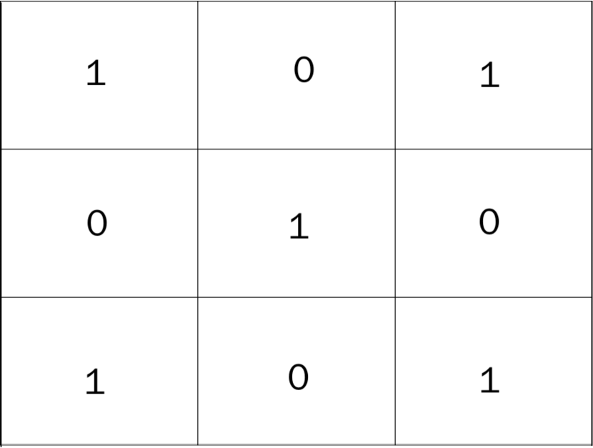
Figure 1: This picture illustrates the spatial distribution of the part of SEP source near the Sun. The area of source is divided evenly in latitudes and longitudes. The regions filled with ions are marked as “1”; the regions devoid of ions are marked as “0”.

The particle source on the solar wind source surface covers certain ranges of longitudinal and latitudinal $S_{long}\times S_{lat}$. The spatial distribution of the SEP source is shown in Figure 1. The source region is divided into small cells with the same longitude and latitude intervals. The regions filled with ions are labeled as “1”, and the regions devoid of ions are labeled as “0”. The size of every cell is set as $1.5^{\circ}$ in both latitudinal and longitudinal direction. This setup of source region is to mimic the effect of braided magnetic field lines due to random walk of foot-point in the low corona. The size of the cell is equivalent to the typical size of supergranular motion. Without perpendicular diffusion, the particles propagate outward from the source to the interplanetary space only along the field lines. In this case, only the magnetic flux tubes connected to the regions labelled as “1” in the phase of source particle injection are filled with particles, and the rest of tubes are devoid of particles. As the magnetic flux tubes past by an observer at 1 AU, the observer can see alternating switch-ons and switch-offs of SEPs. However, with perpendicular diffusion, particles can cross the field lines when they propagate in the interplanetary space. In this case, the longitudinal gradients in the particle intensities at different locations of interplanetary space will be reduced.

We use boundary values to model the particles’ injection from the source. The source rotates with the Sun, and the boundary condition is chosen as the following form

$${f_{b}}(z\leq 0.05AU,{E_{k}},\theta,\varphi,t)=\frac{a}{t}\cdot\frac{{E_{k}^{-\gamma}}}{{{p^{2}}}}\cdot\exp\left({-\frac{{{t_{c}}}}{t}-\frac{t}{{{t_{l}}}}}\right)\cdot\xi,$$ (6)

$$\xi\left({\theta,\varphi}\right)=\left\{{\begin{array}[]{*{20}{l}}{{e^{(-a\phi/\phi_{0})}}{\kern 15.0pt}\textrm{in source region 1}}\\ {0{\kern 15.0pt}\textrm{otherwise}}\end{array}}\right.$$

where the particles are injected from the SEP source near the Sun. $\xi$ indicates the spatial scale of every cell. $E_{k}$ is the particles energy. We set a typical value of $\gamma=-3$ for the spectral index of source particles. Because of adiabatic energy loss, those particles observed at $1$ AU have less energy than their initial energy at the source. In our simulations, energy of particles at source are just a few times larger than that of particles at $1$ AU. Time constants $t_{c}=0.48$ hour and $t_{l}=1.24$ hours indicate the rise and decay time scales, respectively. The injection time scales are used to model an impulsive SEP event. $\phi$ is the angle distance from the center of the cell and where the particles are injected. $\phi_{0}$ and $a$ are the constant. $\phi_{0}$ is set to be $0.75^{\circ}$ (the half width of each cell), but $a$ is allowed to change according to several different scenarios. The inner boundary is 0.05 AU and the outer boundary is 50 AU. The transport equation (1) is solved by a time-backward Markov stochastic process method (Zhang, 1999; Qin et al., 2006). The transport equation can be reformulated to stochastic differential equations, so it can be solved by a Monte-Carlo simulation of Markov stochastic process, and the SEP distribution function can be derived. In this method, we trace virtual particles from the observation point back to the injection time from the SEP source. More details of the technique can be found in those references.

3 RESULTS

3.1 ${\kappa_{\bot}}/{\kappa_{\parallel}}$ Ratio

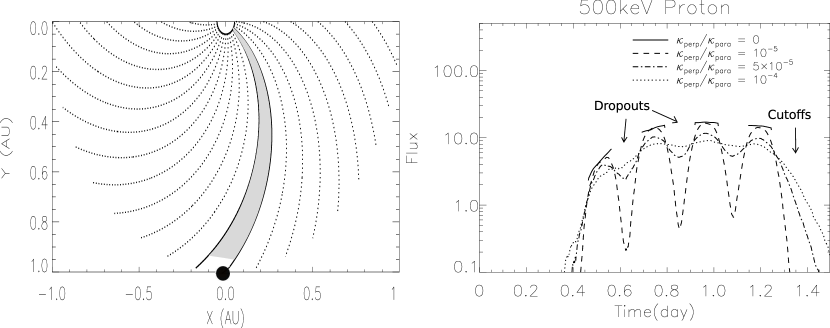
Figure 2: The left panel illustrates the spatial distribution of magnetic field lines in the interplanetary space. The area of source is divided evenly in latitudes and longitudes. The interplanetary magnetic field is set as the Parker model.The grey region indicates that the field lines connected to the source. The observer is located at $1$ AU in the ecliptic as indicated by the black circle. In the right panel, $500$ keV proton fluxes with different perpendicular diffusion are calculated. The $\lambda_{\parallel}$ is equal to $0.087$ $AU$, and the source parameter $a$ is set as $0$ in all cases. Different lines correspond to the different ratios of perpendicular diffusion coefficient to the parallel one: $\kappa_{\perp}/\kappa_{\parallel}=0$ (solid line); $\kappa_{\perp}/\kappa_{\parallel}=1\times 10^{-5}$ (dash line); $\kappa_{\perp}/\kappa_{\parallel}=5\times 10^{-5}$ (dash dot line); and $\kappa_{\perp}/\kappa_{\parallel}=1\times 10^{-4}$ (dot line).

Figure 2 shows the interplanetary magnetic field in the ecliptic in the left panel, and the omni-directional fluxes for $500$ keV protons which are detected at $1$ AU in the right panel. In the left panel, the grey region indicates that the field lines are connected to the source. The dropouts and cutoffs are interpreted as the magnetic flux tubes which are alternately filled with and devoid of ions pass the spacecraft. In our model, the source rotates with the Sun. As a result, the magnetic flux tube which connects with the source also rotates with the source. The observer is located at $1$ AU ($x=0,y=1$) in the equatorial plane as indicated by the black circle. The magnetic flux tubes rotate with the Sun, and the angular speed is $0.55^{\circ}$ per hour. According to the typical size of supergranulation, the size of every cell is set as $1.5^{\circ}$ in both latitudinal and longitudinal direction. An observer in the ecliptic traverses a cell in nearly $2.7$ hours. Due to the connection of the magnetic flux tubes, the observer’s field lines can connect to different regions which are alternately filled with and devoid of ions. In the right panel, the source parameter $a$ is set as $0$, so the source intensity is uniform in every cell. The source width is $S_{long}=S_{lat}=18^{\circ}$. When the particles are injected, the observer at $1$ AU is magnetically connected with the first boundary of the source region. This same magnetic connection is also verified for the other simulations, except the last one when the observer is located at larger distance. In all the cases, the parallel mean free paths are the same (${\lambda_{\parallel}=0.087}$ AU), but the perpendicular diffusion coefficients, and subsequently the ratios of perpendicular diffusion coefficients to parallel ones, are set to several different values. With perpendicular diffusion, particles can be detected even if the observer is not connected directly to region 1 by field lines. The observer detects enhancements of particles starting at nearly $0.3$ day after the particles are injected on the Sun. With a larger perpendicular diffusion, the onset time of flux changes to an earlier time. The onset time of flux is the earliest and the latest in the cases of ${\kappa_{\perp}}/{\kappa_{\parallel}}=1\times 10^{-4}$ and ${\kappa_{\bot}}/{\kappa_{\parallel}}=0$, respectively. During the time interval from $0.55$ to $0.65$ day, the observer’s field lines are connected to region 0. Without perpendicular diffusion, the observer can not detect energetic particles, so the flux suddenly drops to zero. As the ${\kappa_{\bot}}/{\kappa_{\parallel}}$ increases from $0$ to $1\times 10^{-4}$, the variation of flux becomes increasingly smaller during the interval from $0.55$ to $0.65$ day. Especially in the case of ${\kappa_{\bot}}/{\kappa_{\parallel}}=1\times 10^{-4}$, there is essentially no difference in the flux between the time intervals when the observer’s field lines are not connected to the source. Later on, when the observer is connected to the region $0$ again during the time interval from $0.8$ to $0.9$ day, the fluxes behave similarly to those in the interval from $0.55$ to $0.65$ day. After $1.25$ day, the observer is completely disconnected from the source region. The flux decreases very quickly in the case of ${\kappa_{\bot}}/{\kappa_{\parallel}}=1\times 10^{-5}$, but the decreases slow down as the perpendicular diffusion coefficient increases. The time between neighboring valleys and peaks is less than $3$ hours. Let us define a ratio $R_{i}=f_{p,i}/f_{v,i}$, where $f_{p,i}$ and $f_{v,i}$ are the ith peak value and valley value of the flux, respectively. If the ratio $R_{i}$ is larger than $2$, we count it as a dropout. Since the ratios $R_{i}$ in each of the valleys are similar, we only use the ratio $R_{2}$ to identify the dropouts of the fluxes. When ${\kappa_{\bot}}/{\kappa_{\parallel}}$ is set as $0$, $1\times 10^{-5}$, and $5\times 10^{-5}$, $R_{2}$ is approximately equal to $+\infty$, $30.4$, and $2.2$, respectively. We find that the dropouts can be reproduced only in the cases with ${\kappa_{\bot}}/{\kappa_{\parallel}}\lesssim 5\times 10^{-5}$. In any case, if a dropout is reproduced, a cutoff, the step-like intensities decrease without recovery, is also reproduced. In this sense, dropouts and cutoffs are the same phenomenon, with the only difference being whether or not the flux is recovered by a follow-on connection to the particle source.

3.2 Parallel Mean Free Path

The level of parallel mean free path affects the speed of particle propagation from the Sun to the Earth. Figure 3 is similar to Figure 2 but with different turbulence parameters $A_{1}$ or parallel mean free paths. The left panel corresponds to ${\lambda_{\parallel}}=0.0{\rm{26}}$ AU, and the right panel is corresponding to ${\lambda_{\parallel}}=0.{\rm{5}}$ AU. Due to the smaller parallel mean free path in the left panel of Figure 3, the onset of the fluxes shifts to a later time than that in Figure 2. In the right panel, where the mean free path is larger than that in Figure 2, the onset is earlier. In the left panel, the observer only detects two dropouts, then its foot-point goes away becomes disconnected from the source region. However, due to a larger parallel mean free path, the observer detects four dropouts in the right panel. When ${\kappa_{\bot}}/{\kappa_{\parallel}}$ is set as $1\times 10^{-5}$ and $5\times 10^{-5}$, $R_{2}$ is approximately equal to $560$ and $3.7$ in the left panel, and is approximately equal to $5.5$ and $1.5$ in the right panel, respectively. The dropouts requires ${\kappa_{\bot}}/{\kappa_{\parallel}}\lesssim 5\times 10^{-5}$ in the case of ${\lambda_{\parallel}}=0.0{\rm{26}}$ AU, and requires ${\kappa_{\bot}}/{\kappa_{\parallel}}\lesssim 1\times 10^{-5}$ in the case of ${\lambda_{\parallel}}=0.{\rm{5}}$ AU. Otherwise, the dropouts disappear. The results show that the upper limit of ${\kappa_{\bot}}/{\kappa_{\parallel}}$ in dropouts changes little with different ${\lambda_{\parallel}}$. The relation of the appearance of dropout and parallel mean free path at given ${\kappa_{\bot}}/{\kappa_{\parallel}}$ ratio can be understood as follows. When the mean free path increase, it takes a shorter time for the particles to propagate from the Sun to the Earth, during which the particle can not diffuse across magnetic field lines too much even with a large perpendicular diffusion coefficient. Therefore, it is the ratio of ${\kappa_{\bot}}/{\kappa_{\parallel}}$ that determines whether a dropout of particle intensity is observed at the distance of 1 AU.

3.3 Spatial Variation of SEP Source

The left panel of Figure 4 is the same as Figure 2. In the right panel, the source region is set to $S_{long}=S_{lat}=15^{\circ}$ which is narrower than that in the left panel. Due to a narrower source, the observer only encounters two dropouts instead of three. Other than this, the fluxes in the right panel of Figure 4 show behaviors similar to those in left panel.

Figure 5 shows $500$ keV proton fluxes with different spatial distribution of source. The four panels (a), (b), (c), and (d) correspond to $\kappa_{\perp}/\kappa_{\parallel}=0$, $\kappa_{\perp}/\kappa_{\parallel}=1\times 10^{-5}$, $\kappa_{\perp}/\kappa_{\parallel}=5\times 10^{-5}$, and $\kappa_{\perp}/\kappa_{\parallel}=1\times 10^{-4}$, respectively. In every panel, the source parameter $a$ varies from $0$ to $12$. With a larger parameter $a$, the source intensity decreases more quickly towards the flank of each cell. In the panel (a), the ${\kappa_{\bot}}/{\kappa_{\parallel}}$ is set as $0$. No particle is detected by the observer when the field line is disconnected from the source. In the panel (b), the ${\kappa_{\bot}}/{\kappa_{\parallel}}$ is set as $1\times 10^{-5}$. Due to the variation of source intensity, the fluxes observed at 1 AU drop much more as $a$ increases. When $a$ increases from $0$ to $12$, $R_{2}$ also increase from $30.4$ to $1962$. In the panel (c), the ${\kappa_{\bot}}/{\kappa_{\parallel}}$ is set as $5\times 10^{-5}$. The fluxes observed at 1 AU drop much slower as $a$ increases than that in the panel (b). When $a$ is set as $0$, $3$, $6$, and $12$, $R_{2}$ is approximately equal to $2.2$, $2.7$, $3.3$, and $3.6$. In the panel (d), the ${\kappa_{\bot}}/{\kappa_{\parallel}}$ is set as $1\times 10^{-4}$. There is no significant difference in the fluxes observed at 1 AU as $a$ increases. Based on the results in the four panels, we find that the dropouts can be detected in the cases with a slightly higher ratio of ${\kappa_{\bot}}/{\kappa_{\parallel}}\lesssim 5\times 10^{-5}$, if the source distribution becomes narrower.

3.4 Energy Dependence of Dropouts and Cutoffs

The left panel of Figure 6 is the same as Figure 2. The right panel of Figure 6 shows the omni-directional flux for 5 MeV protons detected at 1 AU in the ecliptic. The parallel mean free paths remain the same (${\lambda_{\parallel}}=0.{\rm{13}}$ AU at $1$ AU) in all cases, but the perpendicular diffusion coefficient is set to several different values. The source width in the two panels are set as $S_{long}=S_{lat}=18^{\circ}$. The source parameter $a$ is set as $0$ in the two panels. Comparing with the left panel, the onset time of flux is earlier because of the higher energy and the larger parallel mean free path in the right panel. In the right panel, when ${\kappa_{\bot}}/{\kappa_{\parallel}}$ is set as $0$, $1\times 10^{-5}$, and $5\times 10^{-5}$, $R_{2}$ is approximately equal to $+\infty$, $10$, and $1.7$, respectively. The dropouts can be reproduced in the cases of ${\kappa_{\bot}}/{\kappa_{\parallel}}\lesssim 1\times{10^{-5}}$ in the right panel. As a comparison, in the left panel, dropouts can be reproduced in the cases of ${\kappa_{\bot}}/{\kappa_{\parallel}}\lesssim 5\times{10^{-5}}$.

3.5 Observer at A Larger Radial Distance

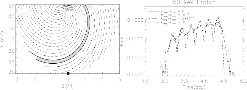
Figure 7: The left panel illustrates the spatial distribution of magnetic field lines in the interplanetary space. The observer is located at 3 AU in the ecliptic as indicated by the black circle. In the right panel, $500$ keV proton fluxes with different perpendicular diffusion are caculated. The $\lambda_{\parallel}$ is equal to $0.087$ $AU$, and the source parameter $a$ is set as $0$ in all cases.

Results for an observer at $3$ AU in the ecliptic are shown in the Figure 7. The left panel illustrates the interplanetary magnetic field lines. Due to a larger radial distance, the particles spend more time propagating from the source to the observer than in the case of $1$ AU. In order to detect the particles, the foot-point of observer is set as west $40^{\circ}$ to the boundary of source at the beginning of the simulation. In the right panel, the onset of the fluxes shifts to a later time than that in Figure 2. As the source rotates with the Sun, the observer encounters five dropouts, which is more than seen in Figure 2, because the observer is located at the boundary of the source at the initial time in Figure 2, and particles spend some time propagating from source to $1$ AU. As a results, the observer missed two dropouts in Figure 2. In the right panel of Figure 7, the dropouts can be detected in the cases of ${\kappa_{\bot}}/{\kappa_{\parallel}}\lesssim 1\times{10^{-5}}$. In the case of ${\kappa_{\bot}}/{\kappa_{\parallel}}=5\times{10^{-5}}$, the dropout is absent in Figure 7, but it appears in Figure 2. The reason is that it takes a longer time for the particles to propagate from the Sun to the observer, and for perpendicular diffusion to be effective, when the solar radial distance increases.

4 DISCUSSIONS AND CONCLUSIONS

By numerically solving the Fokker-Planck focused transport equation for $500$ keV and $5$ MeV protons, we have investigated the effect of the perpendicular diffusion coefficients on the dropouts and cutoffs when an observer is located at $1$ AU or $3$ AU in the ecliptic. SEPs are injected from a source near the Sun, and the source rotates with the Sun. The dropouts and cutoffs are caused by the magnetic flux tubes which are alternately filled with and devoid of ions past the spacecraft. In this paper, all the times between neighbouring valleys and peaks are less than $3$ hours, and the ratio $R_{2}$ between the second peak value and the second valley value are used to identify the dropouts. The dropout is defined to be present when $R_{2}$ is more than a significant factor, which is set to be 2. We list the values of $R_{2}$ in the cases of different magnetic field turbulence intensities in Table 1.

Our simulations are performed for several different parallel mean free paths (${\lambda_{\parallel}}=$ $0.5$ AU, $0.087$ AU, $0.026$ AU at $1$ AU) with different assumption for the ratios of perpendicular diffusion coefficient to the parallel one. With a larger parallel mean free path, the onset time of SEP flux appears earlier, and more dropouts can be detected. Meanwhile, the flux increases more quickly, and the peak time is also earlier. This feature is closely related to the pitch angle distribution of particles arriving at the observer. Since the particles encounter fewer scatterings when they propagate in the interplanetary space with a larger parallel mean free path. Therefore, the distribution of pitch angle would be anisotropic for a longer time in this case. In order to reproduce the dropouts and cutoffs at 1 AU, the perpendicular diffusion has to be small: ${\kappa_{\bot}}/{\kappa_{\parallel}}\lesssim 5\times{10^{-5}}$ when observer is located at $1$ AU, while ${\kappa_{\bot}}/{\kappa_{\parallel}}\lesssim 1\times{10^{-5}}$ when observer is located at $3$ AU. In any case when the dropouts are reproduced, cutoffs can also be reproduced when the observer’s flux tubes completely move out of the source region. If the observer is located at a larger radial distance (eg, $3$ AU in our simulation), it takes a longer time for the particles to propagate from the Sun to the observer, and perpendicular diffusion has more time to be effective. In order to reproduce the dropout at several AU, the ratio of ${\kappa_{\bot}}/{\kappa_{\parallel}}$ should be lower than that in the cases of $1$ AU. As a result, our simulation also predicts that the dropout may disappear at larger radial distances, which can be checked by analysing data from Ulysses or other spacecraft at large distance.

With a wider source, the observer can detect more dropouts. Other than this, the fluxes with a wider source show behaviors similar to those with a narrower source. As $a$ changes from $0$ to $12$, in the case of ${\kappa_{\bot}}/{\kappa_{\parallel}}=1\times{10^{-5}}$, the ratio $R_{i}$ is much larger in the case of $a=12$ than that in the case of $a=0$. However, in the cases of ${\kappa_{\bot}}/{\kappa_{\parallel}}=1\times{10^{-4}}$ and ${\kappa_{\bot}}/{\kappa_{\parallel}}=5\times{10^{-5}}$, the ratio $R_{i}$ does not change significantly as $a$ changes from $0$ to $12$.

For $5$ MeV protons, the case of ${\lambda_{\parallel}}=0.13$ AU has been analysed. Due to the higher particle speed and a typically larger parallel mean free path, the onset time appears earlier than for $500$ keV protons. As a result, more dropouts can be detected. In order to reproduce the dropouts and cutoffs, the ratio of the perpendicular diffusion coefficient to the parallel one should be smaller than $10^{-5}$, which is a little lower than that in the cases for $500$ keV protons.

Different ${\kappa_{\bot}}$ and ${\kappa_{\parallel}}$ are obtained by altering the parameters $A_{1}$ and $A_{2}$ in our simulations, respectively, where ${A_{1}}={\left({\delta{B_{slab}}}\right)^{2}}/({{{B_{0}}}^{2}}\cdot l_{slab})$, and ${A_{2}}={\left({\delta{B_{2D}}}\right)^{2}}/{\left({{B_{0}}}\right)^{2}}\cdot{l_{2D}}$. In Table 1, we list all coefficients in the diffusion formulae which are used in our simulations with $\lambda_{\parallel}$ equal to $0.5$ AU, $0.087$ AU, $0.026$ AU for $500$ keV protons and $0.13$ AU for $5$ MeV protons at $1$ AU. In this table, we assume a slab turbulence correlation length $l_{slab}=0.03$ AU, and 2D correlation length $l_{2D}=0.003$ AU. As we can see, the ${\left({\delta{B_{slab}}/{B_{0}}}\right)^{2}}$ is much larger than ${\left({\delta{B_{2D}}/{B_{0}}}\right)^{2}}$ in all cases. This result is consistent with the observation (Tan et al., 2014). However, we should note that the exact values of ${\left({\delta{B_{slab}}/{B_{0}}}\right)^{2}}$, ${\left({\delta{B_{2D}}/{B_{0}}}\right)^{2}}$, $l_{slab}$ and $l_{2D}$ cannot be well determined. For example, we can assume slab turbulence correlation length $l_{slab}=0.003$ AU instead, and ${\lambda_{\parallel}}=0.5$ AU, $0.087$ AU, and $0.026$ AU for $500$ keV protons given ${\left({\delta{B_{slab}}/{B_{0}}}\right)^{2}}=0.05$, $0.3$, and $1$, respectively. In our results we need a very small $\delta B_{2D}/\delta B_{slab}$ to get a small perpendicular diffusion coefficients from the NLGC theory. However, the NLGC results with a small $\delta B_{2D}/\delta B_{slab}$ are much larger than simulation results (e.g., Qin, 2007). Although $\delta B_{2D}/\delta B_{slab}$ must be small to get the small perpendicular diffusion coefficients, the actual value of $\delta B_{2D}/\delta B_{slab}$ needed according to simulations (Qin, 2007) is not as extremely small as that shown in Table 1 from NLGC theory.

In Dröge et al. (2010), the cutoffs can be reproduced for a ratio of ${\kappa_{\bot}}/{\kappa_{\parallel}}$ a few times $10^{-5}$. This ratio is similar to what we deduced from our simulations. The basic difference between this simulation and the one in Dröge et al. (2010) is that we reproduced the dropouts and cutoffs simultaneously, while their simulation only reproduced the cutoffs. We believe that the cutoffs are only a special type of dropout in which the intensity suddenly decreases without recovery. In Giacalone et al. (2000) and Guo & Giacalone (2014), perpendicular diffusion coefficients relative to the background magnetic field (instead of Parker spiral) needed to be very small for reproducing the dropouts. That is consistent with our results. It should be noted that in our model, the large scale magnetic field is assumed to be a Parker spiral so that the Fokker-Planck focused transport equation can be solved efficiently with our stochastic method. In reality, the magnetic field lines with randomly walking foot-point do not have an azimuthal symmetry. However the large-scale geometry of interplanetary magnetic field and the behaviours of particle transport in it are not much different from those with a Parker magnetic field. The only difference is a slight shift of SEP source location relative to the magnetic field line passing through the observation at 1 AU.

Some special sets of turbulence parameters are needed in our simulations to produce small perpendicular diffusion coefficients in order to produce the dropouts and cutoffs. For example, turbulence dominated by a slab component leads to very small perpendicular diffusion coefficients. In the future, it will be interesting for us to study solar wind turbulence geometry from spacecraft observations when SEP dropouts and cutoffs occur.

Figure 3: Similar to Figure 2 but with different diffusion coefficients. The $\lambda_{\parallel}$ is $0.026$ AU in the left panel, and is $0.5$ AU in the right panel. The source parameter $a$ is set as $0$ in all cases.

Figure 4: Comparison of $500$ keV proton fluxes with different source width. The width of source is $S_{long}=S_{lat}=18^{\circ}$ in the left panel, and is $S_{long}=S_{lat}=15^{\circ}$ in the right panel. The $\lambda_{\parallel}$ is equal to $0.087$ $AU$, and the source parameter $a$ is set as $0$ in all cases.

Figure 5: Comparison of $500$ keV proton fluxes with different spatial distribution of source. The source parameter $a$ changes from $0$ to $12$ in every panel. The four panels (a), (b), (c), and (d) are corresponding to $\kappa_{\perp}/\kappa_{\parallel}=0$, $\kappa_{\perp}/\kappa_{\parallel}=1\times 10^{-5}$, $\kappa_{\perp}/\kappa_{\parallel}=5\times 10^{-5}$, and $\kappa_{\perp}/\kappa_{\parallel}=1\times 10^{-4}$, respectively. The $\lambda_{\parallel}=0.087$ AU in the four panels.

Figure 6: Comparison of 500 keV proton fluxes (the left panel) with 5 MeV proton fluxes (the right panel). The source parameter $a$ is set as $0$ in the two panels.

Table 1: Diffusion coefficients and flux ratios.

${\lambda_{\parallel}}$ $(AU)$	$l_{slab}$ $(AU)$	$l_{2D}$ $(AU)$	${\left({\delta{B}/{B_{0}}}\right)^{2}}$	${\kappa_{\bot}}/{\kappa_{\parallel}}$	${\left({\delta{B_{2D}}/{B_{slab}}}\right)^{2}}$	${R_{2}}^{c}$
$0.5^{a}$	$3\times{10^{-2}}$	$3\times{10^{-3}}$	0.05	0	0	$+\infty$
				$1\times 10^{-5}$	$1\times 10^{-5}$	$5.5$
				$5\times 10^{-5}$	$9\times 10^{-5}$	$1.5$
				$1\times 10^{-4}$	$3\times 10^{-4}$	$1.5$
$0.087^{a}$	$3\times{10^{-2}}$	$3\times{10^{-3}}$	0.3	0	0	$+\infty$
				$1\times 10^{-5}$	$2\times 10^{-6}$	$30.4$
				$5\times 10^{-5}$	$2\times 10^{-5}$	$2.2$
				$1\times 10^{-4}$	$5\times 10^{-5}$	$1.1$
$0.026^{a}$	$3\times{10^{-2}}$	$3\times{10^{-3}}$	1	0	0	$+\infty$
				$1\times 10^{-5}$	$4\times 10^{-7}$	$560$
				$5\times 10^{-5}$	$5\times 10^{-6}$	$3.7$
				$1\times 10^{-4}$	$1\times 10^{-5}$	$1.4$
$0.13^{b}$	$3\times{10^{-2}}$	$3\times{10^{-3}}$	0.3	0	0	$+\infty$
				$1\times 10^{-5}$	$2\times 10^{-6}$	$10$
				$5\times 10^{-5}$	$2\times 10^{-5}$	$1.7$
				$1\times 10^{-4}$	$7\times 10^{-5}$	$1.3$

References

- Beeck & Wibberenz (1986) Beeck, J., & Wibberenz, G. 1986, ApJ, 311, 437
- Bieber et al. (1994) Bieber, J.W, Matthaeus, W.H., Smith, C.W., Wanner, W., Kallenrode, M.-B., & Wibberenz, G. 1994, The Astrophysical Journal, 420, 294
- Chollet & Giacalone (2008) Chollet, E., & Giacalone, J. 2008, The Astrophysical Journal, 688, 1368
- Chuychai et al. (2007) Chuychai, P., Ruffolo, D., Matthaeus, W. H., & Meechai, J. 2007, ApJ, 659, 1761
- Chuychai et al. (2005) Chuychai, P., Ruffolo, D., Matthaeus, W. H., & Rowlands, G. 2005, ApJ, 633, L49
- Dröge et al. (2010) Dröge, W., Kartavykh, Y., Klecker, B., & Kovaltsov, G. 2010, The Astrophysical Journal, 709, 912
- Earl (1974) Earl, J. 1974, The Astrophysical Journal, 193, 231
- Giacalone et al. (2000) Giacalone, J., Jokipii, J., & Mazur, J. 2000, The Astrophysical Journal Letters, 532, L75
- Gosling et al. (2004) Gosling, J. T., Skoug, R. M., McComas, D. J., & Mazur, J. E. 2004, ApJ, 614, 412
- Guo & Giacalone (2014) Guo, F., & Giacalone, J. 2014, The Astrophysical Journal, 780, 16
- He et al. (2011) He, H.-Q., Qin, G., & Zhang, M. 2011, ApJ, 734, 74
- Jokipii (1966) Jokipii, J. R. 1966, ApJ, 146, 480
- Kaghashvili et al. (2006) Kaghashvili, E. K., Zank, G. P., & Webb, G. M. 2006, ApJ, 636, 1145
- Matthaeus et al. (1990) Matthaeus, W. H., Goldstein, M. L., & Roberts, D. A. 1990, Journal of Geophysical Research, 95, 20673
- Matthaeus et al. (2003) Matthaeus, W. H., Qin, G., Bieber, J. W., & Zank, G. P. 2003, ApJ, 590, L53
- Mazur et al. (2000) Mazur, J., Mason, G., Dwyer, J., Giacalone, J., Jokipii, J., & Stone, E. 2000, The Astrophysical Journal Letters, 532, L79
- Palmer (1982) Palmer, I.D. 1982, Rev. Geophys. Space Phys., 20, 335
- Qin et al. (2005) Qin, G., Zhang, M., Dwyer, J. R., Rassoul, H. K., Masson, G. M. 2005, ApJ, 627, 562
- Qin et al. (2006) Qin, G., Zhang, M., & Dwyer, J. R. 2006, J. Geophys. Res., 111, 8101
- Qin (2007) Qin, G. 2007, ApJ, 656, 217
- Qin & Shalchi (2009) Qin, G. & Shalchi, A. 2009, ApJ, 707, 61
- Qin & Shalchi (2014) Qin, G. & Shalchi, A. 2014, Physics of Plasmas, 21, 042906
- Qin et al. (2013) Qin, G., Wang, Y., Zhang, M., & Dalla, S. 2013, The Astrophysical Journal, 766, 74
- Ruffolo et al. (2003) Ruffolo, D., Matthaeus, W. H., & Chuychai, P. 2003, ApJ, 597, L169
- Schlickeiser (2002) Schlickeiser, R. 2002, Cosmic ray astrophysics (Springer Verlag)
- Seripienlert et al. (2010) Seripienlert, A., Ruffolo, D., Matthaeus, W. H., & Chuychai, P. 2010, ApJ, 711, 980
- Shalchi et al. (2004) Shalchi, A., Bieber, J., Matthaeus, W., & Qin, G. 2004, The Astrophysical Journal, 616, 617
- Shalchi et al. (2010) Shalchi, A., Li, G., & Zank, G. 2010, Astrophysics and Space Science, 325, 99
- Skilling (1971) Skilling, J. 1971, ApJ, 170, 265
- Tan et al. (2014) Tan, L. C., Reames, D. V., Ng, C. K., Shao, X., & Wang, L. 2014, ApJ, 786, 122
- Teufel & Schlickeiser (2003) Teufel, A., & Schlickeiser, R. 2003, Astronomy and Astrophysics, 397, 15
- Trenchi et al. (2013a) Trenchi, L., Bruno, R., Telloni, D., D’amicis, R., Marcucci, M., Zurbuchen, T., & Weberg, M. 2013a, The Astrophysical Journal, 770, 11
- Trenchi et al. (2013b) Trenchi, L., Bruno, R., D’Amicis, R., Marcucci, M., & Telloni, D. 2013b, Annales Geophysicae 31, 1333
- Wang et al. (2012) Wang, Y., Qin, G., & Zhang, M. 2012, The Astrophysical Journal, 752, 37
- Zhang (1999) Zhang, M. 1999, ApJ, 513, 409
- Zhang et al. (2009) Zhang, M., Qin, G., & Rassoul, H. 2009, ApJ, 692, 109
- Zuo et al. (2013) Zuo, P., Zhang, M., & Rassoul, H. K. 2013, The Astrophysical Journal, 767, 6