The quest for optimal sampling: Computationally efficient, structure-exploiting measurements for compressed sensing

Abstract

An intriguing phenomenon in many instances of compressed sensing is that the reconstruction quality is governed not just by the overall sparsity of the signal, but also on its structure. This paper is about understanding this phenomenon, and demonstrating how it can be fruitfully exploited by the design of suitable sampling strategies in order to outperform more standard compressed sensing techniques based on random matrices.

1 Introduction

Compressed sensing concerns the recovery of signals and images from a small collection of linear measurements. It is now a substantial area of research, accompanied by a mathematical theory that is rapidly reaching a mature state. Applications of compressed sensing can roughly be divided into two areas. First, type I problems, where the physical device imposes a particular type of measurements. This is the case in numerous real-world problems, including medical imaging (e.g. Magnetic Resonance Imaging (MRI) and Computerized Tomography (CT)), electron microscopy, seismic tomography and radar. Second, type II problems, where the sensing mechanism allows substantial freedom to design the measurements so as to improve the reconstructed image or signal. Applications include compressive imaging and fluoresence microscopy.

This paper is devoted to the role of structured sparsity in both classes of problems. It is well known that the standard sparsifying transforms of compressed sensing, i.e. wavelets and their various generalizations, not only give sparse coefficients, but that there is a distinct structure to this sparsity: wavelet coefficients of natural signals and images are far more sparse at fine scales than at coarse scales. For type I problems, recent developments AHPRBreaking ; BAGSAIEP have shown that this structure plays a key role in the observed reconstruction quality. Moreover, the optimal subsampling strategy depends crucially on this structure. We recap this work in this paper.

Since structure is vitally important in type I problems, it is natural to ask whether or not it can be exploited to gain improvements in type II problems. In this paper we answer this question in the affirmative. We show that appropriately-designed structured sensing matrices can successfully exploit structure. Doing so leads to substantial gains over classical approaches in type II problems, based on convex optimization with universal, random Gaussian or Bernoulli measurements, as well as more recent structure-exploiting algorithms – such as model-based compressed sensing BaranuikModelCS , TurboAMP TurboAMP , and Bayesian compressed sensing HeCarinStructCS ; HeCarinTreeCS – which incorporate structure using bespoke recovery algorithms. The proposed matrices, based on appropriately subsampled Fourier/Hadamard transforms, are also computationally efficient

We also review the theory of compressed sensing introduced in AHPRBreaking ; Bastounis with such structured sensing matrices. The corresponding sensing matrices are highly non-universal and do not satisfy a meaningful Restricted Isometry Property (RIP). Yet, recovery is still possible, and is vastly superior to that obtained from standard RIP matrices. It transpires that the RIP is highly undesirable if one seeks to exploit structure by designing appropriate measurements. Thus we consider an alternative that takes such structure into account, known as the RIP in levels Bastounis .

2 Recovery of wavelet coefficients

In many applications of compressed sensing, we are faced with the problem of recovering an image or signal $x$, considered as a vector in $\mathbb{C}^{n}$ or a function in $L^{2}(\mathbb{R}^{d})$, that is sparse or compressible in an orthonormal basis of wavelets. If $\Phi\in\mathbb{C}^{n\times n}$ or $\Phi\in\mathcal{B}(L^{2}(\mathbb{R}^{d}),\ell_{2}(\mathbb{N}))$ (the set of bounded linear operators) is the corresponding sparsifying transformation, then we write $x=\Phi c$, where $c\in\mathbb{C}^{n}$ or $c\in\ell_{2}(\mathbb{N})$ is the corresponding sparse or compressible vector of coefficients. Given a sensing operator $A\in\mathbb{C}^{m\times n}$ or $A\in\mathcal{B}(L^{2}(\mathbb{R}^{d}),\mathbb{C}^{m})$ and noisy measurements $y=Ax+e$ with $\|e\|_{2}\leq\eta$, the usual approach is to solve the $\ell_{1}$-minimization problem:

$$\min_{z\in\mathbb{C}^{n}}\|\Phi z\|_{1}\quad\mbox{s.t.}\quad\|y-Az\|_{2}\leq\eta.$$ (1)

or

$$\inf_{z\in L^{2}(\mathbb{R}^{d})}\|\Phi z\|_{1}\quad\mbox{s.t.}\quad\|y-Az\|_{2}\leq\eta.$$ (2)

Throughout this paper, we shall denote a minimizer of (1) or (2) as $\hat{x}$. Note that (2) must be discretized in order to be solved numerically, and this can be done by restricting the minimization to be taken over a finite-dimensional space spanned by the first $n$ wavelets, where $n$ is taken sufficiently large BAACHGSCS .

As mentioned, compressed sensing problems arising in applications can be divided into two classes:

1. Imposed sensing operators. The operator $A$ is specified by the practical device and is therefore considered fixed. This is the case in MRI – where $A$ arises by subsampling the Fourier transform Lustig3 ; Lustig – as well as other examples, including X-ray CT (see ChartrandCSCTAlg and references therein), radar HermanStrohmerRadar , electron microscopy CSEIT ; leary2013etcs , seismic tomography LinHermanCSSeismic and radio interferometry CSRadioInterferometry .

2. Designed sensing operators. The sensing mechanism allows substantial freedom to design $A$ so as to improve the compressed sensing reconstruction. Some applications belonging to this class are compressive imaging, e.g. the single-pixel camera SinglePixelCamera and the more recent lensless camera Lensless , and compressive fluorescence microscopy Candes_PNAS . In these applications $A$ is assumed to take binary values (typically $\{-1,1\}$), yet, as we will see later, this is not a significant practical restriction.

As stated, the purpose of this paper is to show that insight gained from understanding the application of compressed sensing to type I problems leads to more effective strategies for type II problems.

2.1 Universal sensing matrices

Let us consider type II problems. In finite dimensions, the traditional compressed sensing approach has been to construct matrices $A$ possessing the following two properties. First, they should satisfy the Restricted Isometry Property (RIP). Second, they should be universal. That is, if $\Phi\in\mathbb{C}^{n\times n}$ is an arbitrary isometry, then $A\Phi$ also satisfies the RIP of the same order as $A$. Subject to these conditions, a typical result in compressed sensing is as follows (see FoucartRauhutCSbook , for example): if $A$ satisfies the RIP of order $2k$ with constant $\delta_{2k}<4/\sqrt{41}$ then, for any $x\in\mathbb{C}^{n}$, we have

$$\|x-\hat{x}\|_{2}\leq C\frac{\sigma_{k}(\Phi^{*}x)_{1}}{\sqrt{k}}+D\eta,$$ (3)

where $\hat{x}$ is any minimizer of (1), $C$ and $D$ are positive constants depending only on $\delta_{2k}$ and, for $c\in\mathbb{C}^{n}$,

$$\sigma_{k}(c)_{1}=\inf_{z\in\Sigma_{k}}\|c-z\|_{1},\qquad\Sigma_{k}=\{z\in\mathbb{C}^{n}:\|z\|_{0}\leq k\}.$$

Hence, $x$ is recovered exactly up to the noise level $\eta$ and the error $\sigma_{k}(c)_{1}$ of the best approximation of $c=\Phi^{*}x$ with a $k$-sparse vector. Since $A$ is universal, one has complete freedom to choose the sparsifying transformation $\Phi$ so as to minimize the term $\sigma_{k}(\Phi^{*}x)_{1}$ for the particular signal $x$ under consideration.

Typical examples of universal sensing matrices $A$ arise from random ensembles. In particular, Gaussian or Bernoulli random matrices (with the latter having the advantage of being binary) both have this property with high probability whenever $m$ is proportional to $k$ times by a log factor. For this reason, such matrices are often thought of as ‘optimal’ matrices for compressed sensing.

Remark 1

One significant drawback of random ensembles, however, is that the corresponding matrices are dense and unstructured. Storage and the lack of fast transforms render them impractical for all but small problem sizes. To overcome this, various structured random matrices have also been developed and studied e.g. pseudo-random permutations of columns of Hadamard or DFT (Discrete Fourier Transform) matrices HadamardBlockScrambled ; Lensless . Often these admit fast, $\mathcal{O}\left(n\log n\right)$ transforms. However, the best known theoretical RIP guarantees are usually larger than for (sub)Gaussian random matrices FoucartRauhutCSbook .

2.2 Sparsity structure dependence and the flip test

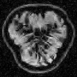
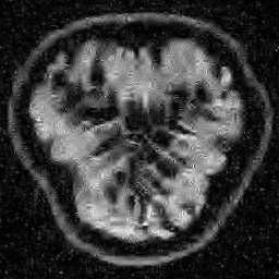
Original image	Gauss. to DB4, err=31.54%	Gauss. to Flip DB4, err=31.51%
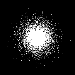
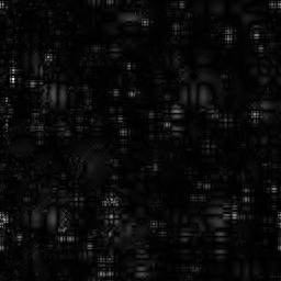
Subsampling pattern	DFT to DB4, err=10.96%	DFT to Flipped DB4, err=99.3%

Figure 1: Recovery of an MRI image of a passion fruit using (1) from $m=8192$ samples at $n=256\times 256$ resolution (i.e. a 12.5% subsampling rate) with Daubechies-4 wavelets as the sparsifying transform $\Phi$. Top row: Flip test for Gaussian random measurements. Botton row: Flip test for subsampled DFT measurements taken according to the subsampling pattern shown in the bottom left panel. The flip test suggests that the RIP holds for random sensing matrices (top row), but that there is no RIP for structured sensing matrices with structured sampling (bottom row).

Since it will become important later, we now describe a quick and simple test, which we call the flip test, to investigate the presence or absence of an RIP. Success of this test suggests the existence of an RIP and failure demonstrates its lack.

Let $A\in\mathbb{C}^{m\times n}$ be a sensing matrix, $x\in\mathbb{C}^{n}$ an image and $\Phi\in\mathbb{C}^{n\times n}$ a sparsifying transformation. Recall that sparsity of the vector $c=\Phi^{*}x$ is unaffected by permutations. Thus, let us define the flipped vector

$$P(c)=c^{\prime}\in\mathbb{C}^{n},\quad c^{\prime}_{i}=c_{n+1-i},\quad i=1,\ldots,n,$$

and using this, we construct the flipped image $x^{\prime}=\Phi c^{\prime}.$ Note that, by construction, we have $\sigma_{k}(c)_{1}=\sigma_{k}(c^{\prime})_{1}$. Now suppose we perform the usual compressed sensing reconstruction (1) on both $x$ and $x^{\prime}$, giving approximations $\hat{x}\approx x$ and $\hat{x}^{\prime}\approx x^{\prime}$. We now wish to reverse the flipping operation. Thus, we compute $\check{x}=\Phi P(\Phi^{*}\hat{x}^{\prime}),$ which gives a second approximation to the original image $x$.

This test provides a simple way to investigate whether or not the RIP holds. To see why, suppose that $A$ satisfies the RIP. Then by construction, we have that

$$\|x-\hat{x}\|_{2},\|x-\check{x}\|_{2}\leq C\frac{\sigma_{k}(\Phi^{*}x)_{1}}{\sqrt{k}}+D\eta.$$

Hence both $\hat{x}$ and $\check{x}$ should recover $x$ equally well. In the top row of Figure 1 we present the result of the flip test for a Gaussian random matrix. As is evident, the reconstructions $\hat{x}$ and $\check{x}$ are comparable, thus indicating the RIP.

Having considered type II problems, let us now examine the flip test for a type I problem. As discussed, in applications such as MRI, X-ray CT, radio interferometry, etc, the matrix $A$ is imposed by the physical sensing device and arises from subsampling the rows of the DFT matrix $F\in\mathbb{C}^{n\times n}$. Whilst one often has some freedom to choose which rows to sample (corresponding to selecting particular frequencies at which to take measurements), one cannot change the matrix $F$.

It is well known that in order to ensure a good reconstruction, one cannot subsample the DFT uniformly at random (recall that the sparsifying transform is a wavelet basis), but rather one must sample randomly according to an appropriate nonuniform density AHPRBreaking ; Candes_Romberg ; Lustig ; WangAcre . See the bottom left panel of Figure 1 for an example of a typical density. As can be seen in the next panel, by doing so one achieves a great recovery. However, the result of the flip test in the bottom right panel clearly demonstrates that the matrix $F\Phi$ does not satisfy an RIP. In particular, the ordering of the wavelet coefficients plays a crucial role in the reconstruction quality. To explain this, and in particular, the high-quality reconstruction seen in the unflipped case, one evidently requires a new analytical framework.

Note that the flip test in Figure 1 also highlights another important phenomenon: namely, the effectiveness of the subsampling strategy depends on the sparsity structure of the image. In particular, two images with the same total sparsity (the original $x$ and the flipped $x^{\prime}$) result in wildly different errors when the same sampling pattern is used. Thus we conclude that there is no one optimal sampling strategy for all sparse vectors of wavelet coefficients.

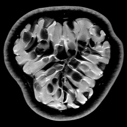
Subsample pattern	Original	TV, err = 9.27%	Permuted gradients	TV, err = 3.83%
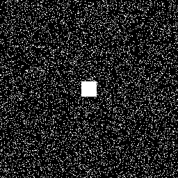
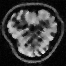
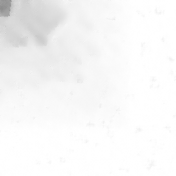
Subsample pattern	Original	TV, err = 28.78%	Permuted gradients	TV, err = 3.76%

Figure 2: TV recovery (4) from $m=16384$ DFT samples at $n=512\times 512$ (6.25% subsampling rate). The Permuted gradients image was built from the same image gradient vectors as the Original image, having the same TV norm and gradient sparsity structure, differing only in the ordering and sign of the gradient vectors. The large error differences confirm that, much like the flip test for wavelet coefficients, the sparsity structure matters for TV reconstructions as well.

Let us also note that the same conclusions of the flip test hold when (1) with wavelets is replaced by TV-norm minimization:

$$\min_{z\in\mathbb{C}^{n}}\|z\|_{TV}\quad\mbox{s.t.}\quad\|y-Az\|_{2}\leq\eta.$$ (4)

Recall that $\|x\|_{TV}=\sum_{i,j}\|\nabla x(i,j)\|_{2}$, where we have $\nabla x(i,j)=\{D_{1}x(i,j),D_{2}x(i,j)\},$ $D_{1}x(i,j)=x(i+1,j)-x(i,j),$ $D_{2}x(i,j)=x(i,j+1)-x(i,j)$. In the experiment leading to Figure 2, we chose an image $x\in[0,1]^{N\times N}$, and then built a different image $x^{\prime}$ from the gradient of $x$ so that $\{\|\nabla x^{\prime}(i,j)\|_{2}\}$ is a permutation of $\{\|\nabla x(i,j)\|_{2}\}$ for which $x^{\prime}\in[0,1]^{N\times N}$. Thus, the two images have the same “TV sparsity” and the same TV norm. In Figure 2 we demonstrate how the errors differ substantially for the two images when using the same sampling pattern. Note also how the improvement depends both on the TV sparsity structure and on the subsampling pattern. Analysis of this phenomenon is work in progress. In the remainder of this paper we will focus on structured sparsity for wavelets.

2.3 Structured sparsity

One of the foundational results of nonlinear approximation is that, for natural images and signals, the best $k$-term approximation error in a wavelet basis decays rapidly in $k$ DeVoreNLACTA ; mallat09wavelet . In other words, wavelet coefficients are approximately $k$-sparse. However, wavelet coefficients possess far more structure than mere sparsity. Recall that a wavelet basis for $L^{2}(\mathbb{R}^{d})$ is naturally partitioned into dyadic scales. Let $0=M_{0}<M_{1}<\ldots<\infty$ be such a partition, and note that $M_{l+1}-M_{l}=\mathcal{O}\left(2^{l}\right)$ in one dimension and $M_{l+1}-M_{l}=\mathcal{O}\left(4^{l}\right)$ in two dimensions. If $x=\Phi c$, let $c^{(l)}\in\mathbb{C}^{M_{l}-M_{l-1}}$ denote the wavelet coefficients of $x$ at scale $l=1,2,\ldots$, so that $c=(c^{(1)}|c^{(2)}|\cdots)^{\top}$. Suppose that $\epsilon>0$ and define

$$k_{l}=k_{l}(\epsilon)=\min\left\{K:\sum^{K}_{i=1}|c^{(l)}_{\pi(i)}|^{2}\geq\epsilon^{2}\|c^{(l)}\|^{2}_{2}\right\},\quad l=1,2,\ldots,$$ (5)

where $\pi$ is a bijection that gives a nonincreasing rearrangement of the entries of $c^{(l)}$, i.e. $|c^{(l)}_{\pi(i)}|\geq|c^{(l)}_{\pi(i+1)}|$ for $i=1,\ldots,M_{l}-M_{l-1}-1$. Sparsity of the whole vector $c$ means that for large $r$ we have $k/n\ll 1$, where $k=k(\epsilon)=\sum^{r}_{l=1}k_{l},$ is the total effective sparsity up to finest scale $r$. However, Figure 3 reveals that not only is this the case in practice, but we also have so-called asymptotic sparsity. That is

$$k_{l}/(M_{l}-M_{l-1})\rightarrow 0,\quad l\rightarrow\infty.$$ (6)

Put simply, wavelet coefficients are much more sparse at fine scales than they are at coarse scales.

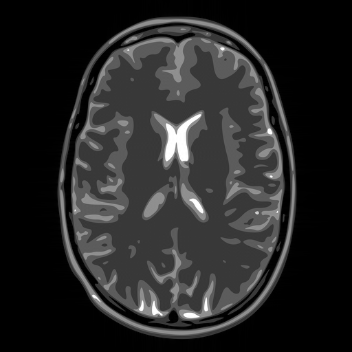
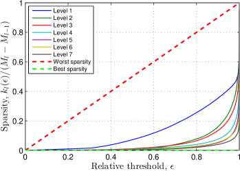
Figure 3: Left: GLPU phantom GLPU . Right: Relative sparsity of Daubechies-4 coefficients. Here the levels correspond to wavelet scales and $k_{l}(\epsilon)$ is given by (5). Each curve shows the relative sparsity at level $l$ as a function of $\epsilon$. The decreasing nature of the curves for increasing $l$ confirms (6).

Note that this observation is by no means new: it is a simple consequence of the dyadic scaling of wavelets, and is a crucial step towards establishing the nonlinear approximation result mentioned above. However, given that wavelet coefficients always exhibit such structure, one may ask the following question. For type II problems, are the traditional sensing matrices of compressed sensing – which, as shown by the flip test (top row of Figure 1), recover all sparse vectors of coefficients equally well, regardless of ordering – optimal when wavelets are used as the sparsifying transform? It has been demonstrated in Figure 1 (bottom row) that structure plays a key role in type I compressed sensing problems. Leveraging this insight, in the next section we show that significant gains are possible for type II problems in terms of both the reconstruction quality and computational efficiency when the sensing matrix $A$ is designed specifically to take advantage of such inherent structure.

Remark 2

Asymptotic sparsity is by no means limited to wavelets. A similar property holds for other types of -lets, including curvelets Cand ; candes2004new , contourlets Vetterli ; Do or shearlets Gitta2 ; Gitta ; Gitta3 (see BAGSAIEP for examples of Figure 3 based on these transforms). More generally, any sparsifying transform that arises (possibly via discretization) from a countable basis or frame will typically exhibit asymptotic sparsity.

Remark 3

Wavelet coefficients (and their various generalizations) actually possess far more structure than the asymptotic sparsity (6). Specifically, they tend to live on rooted, connected trees CrouseEtAlWaveleTree . There are a number of existing algorithms which seek to exploit such structure within a compressed sensing context. We shall discuss these further in Section 5.

3 Efficient sensing matrices for structured sparsity

For simplicity, we now consider the finite-dimensional setting, although the arguments extend to the infinite-dimensional case AHPRBreaking . Suppose that $\Phi\in\mathbb{C}^{n\times n}$ corresponds to a wavelet basis so that $c=\Phi^{*}x$ is not just $k$-sparse, but also asymptotically sparse with the sparsities $k_{1},\ldots,k_{r}$ within the wavelet scales being known. As before, write $c^{(l)}$ for set of coefficients at scale $l$. Considering type II problems, we now seek a sensing matrix $A$ with as few rows $m$ as possible that exploits this local sparsity information.

3.1 Block-diagonality and structured Fourier/Hadamard sampling

For the $l^{\mathrm{th}}$ level, suppose that we assign a total of $m_{l}\in\mathbb{N}$ rows of $A$ in order to recover the $k_{l}$ nonzero coefficients of $c^{(l)}$. Note that $m=\sum^{r}_{l=1}m_{l}$. Consider the product $B=A\Phi$ of the sensing matrix $A$ and the sparsifying transform $\Phi$. Then there is a natural decomposition of $B$ into blocks $\{B_{jl}\}^{r}_{j,l=1}$ of size $m_{j}\times(M_{l}-M_{l-1})$, where each block corresponds to the $m_{j}$ measurements of the $M_{l}-M_{l-1}$ wavelet functions at the $l^{\mathrm{th}}$ scale.

Suppose it were possible to construct a sensing matrix $A$ such that (i) $B$ was block diagonal, i.e. $B_{jl}=0$ for $j\neq l$, and (ii) the diagonal blocks $B_{ll}$ satisfied an RIP of order $2k_{l}$ whenever $m_{l}$ was proportional to $k_{l}$ times by the usual log factor. In this case, one recovers the coefficients $c^{(l)}$ at scale $l$ from near-optimal numbers of measurements using the usual reconstruction (1).

This approach, originally proposed by Donoho donohoCS and Tsaig & Donoho DonohoCSext under the name of ‘multiscale compressed sensing’, allows for structure to be exploited within compressed sensing. Similar ideas were also pursued by Romberg RombergCompImg within the context of compressive imaging. Unfortunately, it is normally impossible to design an $m\times N$ matrix $A$ such that $B=A\Phi$ is exactly block diagonal. Nevertheless, the notion of block-diagonality provides insight into better designs for $A$ than purely random ensembles. To proceed, we relax the requirement of strict block-diagonality, and instead ask whether there exist practical sensing matrices $A$ for which $B$ is approximately block-diagonal whenever the sparsifying transform $\Phi$ corresponds to wavelets. Fortunately, the answer to this question is affirmative: as we shall explain next, and later confirm with a theorem, approximate block-diagonality can be ensured whenever $A$ arises by appropriately subsampling the rows of the Fourier or Hadamard transform. Recalling that the former arises naturally in type I problems, this points towards the previously-claimed conclusion that new insight brought about by studying imposed sensing matrices leads to better approaches for the type II problem.

Let $F\in\mathbb{C}^{n\times n}$ be either the discrete Fourier or discrete Hadamard transform. Let $\Omega\subseteq\{1,\ldots,n\}$ be an index set of size $|\Omega|=m$. We now consider choices for $A$ of the form $A=P_{\Omega}F,$ where $P_{\Omega}\in\mathbb{C}^{m\times n}$ is the restriction operator that selects rows of $F$ whose indices lie in $\Omega$. We seek an $\Omega$ that gives the desired block-diagonality. To do this, it is natural to divide up $\Omega$ itself into $r$ disjoint blocks

$$\Omega=\Omega_{1}\cup\cdots\cup\Omega_{r},\quad|\Omega_{l}|=m_{l},$$

where the $l^{\mathrm{th}}$ block $\Omega_{l}\subseteq\{N_{l-1},\ldots,N_{l}\}$ corresponds to the $m_{l}$ samples required to recover the $k_{l}$ nonzero coefficients at scale $l$. Here the parameters $0=N_{0}<N_{1}<\ldots<N_{r}=n$ are appropriately chosen and delineate frequency bands from which the $m_{l}$ samples are taken.

In Section 3.3, we explain why this choice of $A$ works, and in particular, how to choose the sampling blocks $\Omega_{l}$. In order to do this, it is first necessary to recall the notion of incoherent bases.

3.2 Incoherent bases and compressed sensing

Besides random ensembles, a common approach in compressed sensing is to design sensing matrices using orthonormal systems that are incoherent with the particular choice of sparsifying basis $\Phi$ Candes_Plan ; Candes_Romberg ; FoucartRauhutCSbook . Let $\Psi\in\mathbb{C}^{n\times n}$ be an orthonormal basis of $\mathbb{C}^{n}$. The (mutual) coherence of $\Phi$ and $\Psi$ is the quantity

$$\mu=\mu(\Psi^{*}\Phi)=\max_{i,j=1,\ldots,n}|(\Psi^{*}\Phi)_{i,j}|^{2}.$$

We say $\Psi$ and $\Phi$ are incoherent if $\mu(\Psi,\Phi)\leq a/n$ for some $a\geq 1$ independent of $n$. Given such a $\Psi$, one constructs the sensing matrix $A=P_{\Omega}\Psi,$ where $\Omega\subseteq\{1,\ldots,N\}$, $|\Omega|=m$ is chosen uniformly at random. A standard result gives that a $k$-sparse signal $x$ in the basis $\Phi$ is recovered exactly with probability at least $1-p$, provided

$$m\geq Cka\log(1+p^{-1})\log(n),$$

for some universal constant $C>0$ FoucartRauhutCSbook . As an example, consider the Fourier basis $\Psi=F$. This is incoherent with the canonical basis $\Phi=I$ with optimally-small constant $a=1$. Fourier matrices subsampled uniformly at random are efficient sensing matrices for signals that are themselves sparse.

However, the Fourier matrix is not incoherent with a wavelet basis: $\mu(F,\Phi)=\mathcal{O}\left(1\right)$ as $n\rightarrow\infty$ for any orthonormal wavelet basis AHPRBreaking . Nevertheless, Fourier samples taken within appropriate frequency bands (i.e. not uniformly at random) are locally incoherent with wavelets in the corresponding scales. This observation, which we demonstrate next, explains the success of the sensing matrix $A$ constructed in the previous subsection for an appropriate choice of $\Omega_{1},\ldots,\Omega_{r}$.

3.3 Local incoherence and near block-diagonality of Fourier measurements with wavelets

For expository purposes, we consider the case of one-dimensional Haar wavelets. We note however that the arguments generalize to arbitrary compactly-supported orthonormal wavelets, and to the infinite-dimensional setting where the unknown image $x$ is a function. See Section 4.3.

Let $j=0,\ldots,r-1$ (for convenience we now index from $0$ to $r-1$, as opposed to $1$ to $r$) be the scale and $p=0,\ldots,2^{j}-1$ the translation. The Haar basis consists of the functions $\{\psi\}\cup\{\phi_{j,p}\}$, where $\psi\in\mathbb{C}^{n}$ is the normalized scaling function and $\phi_{j,p}$ are the scaled and shifted versions of the mother wavelet $\phi\in\mathbb{C}^{n}$. It is a straightforward, albeit tedious, exercise to show that

$$|\mathcal{F}\phi_{l,p}(\omega)|=2^{l/2-r+1}\frac{|\sin(\pi\omega/2^{l+1})|^{2}}{|\sin(\pi\omega/2^{r})|}\lesssim 2^{l/2}\frac{|\sin(\pi\omega/2^{l+1})|^{2}}{|\omega|},\quad|\omega|<2^{r},$$

where $\mathcal{F}$ denotes the DFT AHRHaarFourierNote . This suggests that the Fourier transform $\mathcal{F}\phi_{l,p}(\omega)$ is large when $\omega\approx 2^{l}$, yet smaller when $\omega\approx 2^{j}$ with $j\neq l$. Hence we should separate frequency space into bands of size roughly $2^{j}$.

Let $F\in\mathbb{C}^{n\times n}$ be the DFT matrix with rows indexed from $-n/2+1$ to $n/2$. Following an approach of Candes_Romberg , we now divide these rows into the following disjoint frequency bands

$$W_{0}=\{0,1\},\quad W_{j}=\{-2^{j}+1,\ldots,-2^{j-1}\}\cup\{2^{j-1}+1,\ldots,2^{j}\},\quad l=0,\ldots,{r-1}.$$

With this to hand, we now define $\Omega_{j}$ to be a subset of $W_{j}$ of size $|\Omega_{j}|=m_{j}$ chosen uniformly at random. Thus, the overall sensing matrix $A=P_{\Omega}F$ takes measurements of the signal $x$ by randomly drawing $m_{j}$ samples its Fourier transform within the frequency bands $W_{j}$.

Having specified $\Omega$, let us note that the matrix $U=F\Phi$ naturally divides into blocks, with the rows corresponding to the frequency bands $W_{l}$ and the columns corresponding to the wavelet scales. Write $U=\{U_{jl}\}^{r-1}_{j,l=0}$ where $U_{jl}\in\mathbb{C}^{2^{j}\times 2^{l}}$. For compressed sensing to succeed in this setting, we require two properties. First, the diagonal blocks $U_{jj}$ should be incoherent, i.e. $\mu(U_{jj})=\mathcal{O}\left(2^{-j}\right)$. Second, the coherences $\mu(U_{jl})$ of the off-diagonal blocks $U_{jl}$ should be appropriately small in comparison to $\mu(U_{jj})$. These two properties are demonstrated in the following lemma:

Lemma 1

We have $\mu(U_{jj})\lesssim 2^{-j}$ and, in general,

$$\mu(U_{jl})\lesssim\mu(U_{jj})2^{-|j-l|},\quad j,l=0,\ldots,r-1$$

Hence $U$ is approximately block diagonal, with exponential decay away from the diagonal blocks. Fourier measurements subsampled according to the above strategy are therefore ideally suited to recover structured sparse wavelet coefficients.

The left panel of Figure 4 exhibits this decay by plotting the absolute values of the matrix $U$. In the right panel, we also show a similar result when the Fourier transform is replaced by the Hadamard transform. This is an important case, since the measurement matrix is binary. The middle panel of the figure shows the $U$ matrix when Legendre polynomials are used as the sparsifying transform, as is sometimes the case for smooth signals. It demonstrates that diagonally-dominated coherence is not just a phenomenon associated with wavelets.

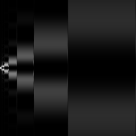
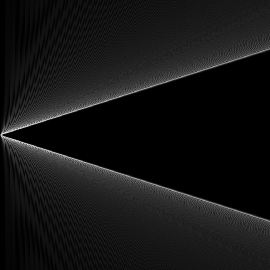
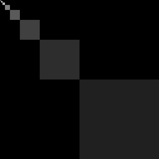
Figure 4: The absolute values of the matrix $U=F\Phi$, where $F$ is the discrete Fourier transform (left and middle) or the Hadamard transform (right) and the sparsifying transform $\Phi$ corresponds to Haar wavelets (left and right) or Legendre polynomials (middle). Light colours correspond to large values and dark colours to small values.

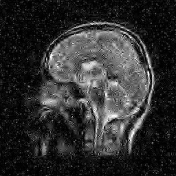
$256\!\times\!256$, err = 41.6%	$512\!\times\!512$, err = 25.3%	$1024\!\times\!1024$, err = 11.6%
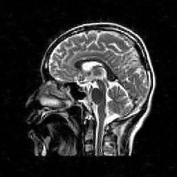
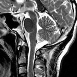
$256\!\times\!256$, err = 21.9%	$512\!\times\!512$, err = 10.9%	$1024\!\times\!1024$, err = 3.1%

Figure 5: Recovery from 12.5% measurements using (1) with Daubechies-4 wavelets as the sparsifying transform. Top row: Random Bernoulli sensing matrix. Bottom row: Fourier sensing matrix with multilevel subsampling (see Definition 3). All images are $256\!\times\!256$ crops of the original full resolution versions in order to aid the visual comparison.

Having identified a measurement matrix to exploit structured sparsity, let us demonstrate its effectiveness. In Figure 5 we compare these measurements with the case of random Bernoulli measurements (this choice was made over random Gaussian measurements because of storage issues). As is evident, at all resolutions we see a significant advantage, since the former strategy exploits the structured sparsity. Note that for both approaches, the reconstruction quality is resolution dependent: the error decreases as the resolution increases, due to the increasing sparsity of wavelet coefficients at higher resolutions. However, because the Fourier/wavelets matrix $U$ is asymptotically incoherent (see also Section 4.1), it exploits the inherent asymptotic sparsity structure (6) of the wavelet coefficients as the resolution increases, and thus gives successively greater improvements over random Bernoulli measurements.

Remark 4

Besides improved reconstructions, an important feature of this approach is storage and computational time. Since $F$ and $\Phi$ have fast, $\mathcal{O}\left(n\log n\right)$, transforms, the matrix $A=P_{\Omega}F\Phi$ does not need to be stored, and the reconstruction (1) can be performed efficiently with standard $\ell_{1}$ solvers (we use SPGL1 SPGL1 ; SPGL1Paper throughout).

Recall that in type I problems such as MRI, we are constrained by the physics of the device to take Fourier measurements. A rather strange conclusion of Figure 5 is the following: compressed sensing actually works better for MRI with the intrinsic measurements, than if one were able to take optimal (in the sense of the standard sparsity-based theory) random (sub)Gaussian measurements. This has practical consequences. In MRI there is actually a little flexibility to design measurements, based on specifying appropriate pulses. By doing this, a number of approaches HaldarRandomEncoding ; ToeplitzMRI ; VanderEtAlSpreadSpectrum ; SebertRandomMRI ; WongMRI have been proposed to make MRI measurements closer to uniformly incoherent with wavelets (i.e. similar to random Gaussians). On the other hand, Figure 5 suggests that one can obtain great results in practice by appropriately subampling the unmodified Fourier operator.

4 A general framework for compressed sensing based on structured sparsity

Having argued for the particular case of Fourier samples with Haar wavelets, we now describe a general mathematical framework for structured sparsity. This is based on work in AHPRBreaking .

4.1 Concepts

We shall work in both the finite- and infinite-dimensional settings, where $U\in\mathbb{C}^{n\times n}$ or $U\in\mathcal{B}(\ell_{2}(\mathbb{N}))$ respectively. We assume throughout that $U$ is an isometry. This occurs for example when $U=\Psi^{*}\Phi$ for an orthonormal basis $\Psi$ and an orthonormal system $\Phi$, as is the case for the example studied in the previous section: namely, Fourier sampling and a wavelet sparsifying basis. However, framework we present now is valid for an arbitrary isometry $U$, not just this particular example. We discuss this case further in Section 4.3.

We first require the following definitions. In the previous section it was suggested to divide both the sampling strategy and the sparse vector of coefficients into disjoint blocks. We now formalize these notions:

Definition 1 (Sparsity in levels)

Let $c$ be an element of either $\mathbb{C}^{N}$ or $\ell_{2}(\mathbb{N})$. For $r\in\mathbb{N}$ let $\mathbf{M}=(M_{1},\ldots,M_{r})\in\mathbb{N}^{r}$ with $1\leq M_{1}<\ldots<M_{r}$ and $\mathbf{k}=(k_{1},\ldots,k_{r})\in\mathbb{N}^{r}$, with $k_{j}\leq M_{j}-M_{j-1}$, $k=1,\ldots,r$, where $M_{0}=0$. We say that $c$ is $(\mathbf{k},\mathbf{M})$-sparse if, for each $j=1,\ldots,r$, the set

$$\Delta_{j}:=\mathrm{supp}(c)\cap\{M_{j-1}+1,\ldots,M_{j}\},$$

satisfies $|\Delta_{j}|\leq k_{j}$. We denote the set of $(\mathbf{k},\mathbf{M})$-sparse vectors by $\Sigma_{\mathbf{k},\mathbf{M}}$.

This definition allows for differing amounts of sparsity of the vector $c$ in different levels. Note that the levels $\mathbf{M}$ do not necessarily correspond to wavelet scales – for now, we consider a general setting. We also need a notion of best approximation:

Definition 2 ($(\mathbf{k},\mathbf{M}$)-term approximation)

Let $c$ be an element of either $\mathbb{C}^{N}$ or $\ell_{2}(\mathbb{N})$. We say that $c$ is $(\mathbf{k},\mathbf{M})$-compressible if $\sigma_{\mathbf{k},\mathbf{M}}(c)$ is small, where

$$\sigma_{\mathbf{k},\mathbf{M}}(c)_{1}=\inf_{z\in\Sigma_{\mathbf{k},\mathbf{M}}}\|c-z\|_{1}.$$ (7)

As we have already seen for wavelet coefficients, it is often the case that $k_{j}/(M_{j}-M_{j-1})\rightarrow 0$ as $j\rightarrow\infty$. In this case, we say that $c$ is asymptotically sparse in levels. However, we stress that this framework does not explicitly require such decay.

We now consider the level-based sampling strategy:

Definition 3 (Multilevel random sampling)

Let $r\in\mathbb{N}$, $\mathbf{N}=(N_{1},\ldots,N_{r})\in\mathbb{N}^{r}$ with $1\leq N_{1}<\ldots<N_{r}$, $\mathbf{m}=(m_{1},\ldots,m_{r})\in\mathbb{N}^{r}$, with $m_{j}\leq N_{j}-N_{j-1}$, $j=1,\ldots,r$, and suppose that

$$\Omega_{j}\subseteq\{N_{j-1}+1,\ldots,N_{j}\},\quad|\Omega_{j}|=m_{j},\quad j=1,\ldots,r,$$

are chosen uniformly at random, where $N_{0}=0$. We refer to the set

$$\Omega=\Omega_{\mathbf{N},\mathbf{m}}=\Omega_{1}\cup\ldots\cup\Omega_{r}.$$

as an $(\mathbf{N},\mathbf{m})$-multilevel sampling scheme.

As discussed in Section 3.2, the (infinite) Fourier/wavelets matrix $U=F\Phi$ is globally coherent. However, as shown in Lemma 1, the coherence of its $(j,l)^{\mathrm{th}}$ block is much smaller. We therefore require a notion of local coherence:

Definition 4 (Local coherence)

Let $U$ be an isometry of either $\mathbb{C}^{N}$ or $\ell_{2}(\mathbb{N})$. If $\mathbf{N}=(N_{1},\ldots,N_{r})\in\mathbb{N}^{r}$ and $\mathbf{M}=(M_{1},\ldots,M_{r})\in\mathbb{N}^{r}$ with $1\leq N_{1}<\ldots N_{r}$ and $1\leq M_{1}<\ldots<M_{r}$ the $(j,l)^{\mathrm{th}}$ local coherence of $U$ with respect to $\mathbf{N}$ and $\mathbf{M}$ is given by

$$\mu_{\mathbf{N},\mathbf{M}}(j,l) =\sqrt{\mu(P^{N_{j-1}}_{N_{j}}UP^{M_{l-1}}_{M_{l}})\mu(P^{N_{j-1}}_{N_{j}}U)},\quad k,l=1,\ldots,r,$$

where $N_{0}=M_{0}=0$ and $P^{a}_{b}$ denotes the projection matrix corresponding to indices $\{a+1,\ldots,b\}$. In the case where $U$ is an operator on $\ell_{2}(\mathbb{N})$, we also define

$$\mu_{\mathbf{N},\mathbf{M}}(j,\infty) =\sqrt{\mu(P^{N_{j-1}}_{N_{j}}UP_{M_{r-1}}^{\perp})\mu(P^{N_{j-1}}_{N_{j}}U)},\quad j=1,\ldots,r.$$

Note that the local coherence $\mu_{\mathbf{N},\mathbf{M}}(j,l)$ is not just the coherence $\mu(P^{N_{j-1}}_{N_{j}}UP^{M_{l-1}}_{M_{l}})$ in the $(j,l)^{\mathrm{th}}$ block. For technical reasons, one requires the product of this and the coherence $\mu(P^{N_{j-1}}_{N_{j}}U)$ in the whole $j^{\mathrm{th}}$ row block.

Remark 5

In KrahmerWardCSImaging , the authors define a local coherence of a matrix $U$ in the $j^{\mathrm{th}}$ row (as opposed to row block) to be the maximum of its entries in that row. Using this, they prove recovery guarantees for the Fourier/Haar wavelets problem based on the RIP and the global sparsity $k$. Unfortunately, these results do not explain the importance of structured sparsity as shown by the flip test. Conversely, our notion of local coherence also takes into account the sparsity levels. As we will see in Section 4.2, this allows one to establish recovery guarantees that are consistent with the flip test and properly explain the role of structure in the reconstruction.

Recall that in practice (see Figure 4), the local coherence often decays along the diagonal blocks and in the off-diagonal blocks. Loosely speaking, we say that the matrix $U$ is asymptotically incoherent in this case.

In Section 3.3 we argued that the Fourier/wavelets matrix was nearly block-diagonal. In our theorems, we need to account for the off-diagonal terms. To do this in the general setup, we require a notion of a relative sparsity:

Definition 5 (Relative sparsity)

Let $U$ be an isometry of either $\mathbb{C}^{N}$ or $\ell_{2}(\mathbb{N})$. For $\mathbf{N}=(N_{1},\ldots,N_{r})\in\mathbb{N}^{r}$, $\mathbf{M}=(M_{1},\ldots,M_{r})\in\mathbb{N}^{r}$ with $1\leq N_{1}<\ldots<N_{r}$ and $1\leq M_{1}<\ldots<M_{r}$, $\mathbf{k}=(k_{1},\ldots,k_{r})\in\mathbb{N}^{r}$ and $j=1,\ldots,r$, the $j^{\mathrm{th}}$ relative sparsity is given by

$$K_{j}=K_{j}(\mathbf{N},\mathbf{M},\mathbf{k})=\max_{\begin{subarray}{c}z\in\Sigma_{\mathbf{k},\mathbf{M}}\end{subarray},\|\eta\|_{\infty}\leq 1}\|P_{N_{j}}^{N_{j-1}}Uz\|^{2},$$

where $N_{0}=M_{0}=0$.

The relative sparsities $K_{j}$ take into account interferences between different sparsity level caused by the non-block diagonality of $U$.

4.2 Main theorem

Given the matrix/operator $U$ and a multilevel sampling scheme $\Omega$, we now consider the solution of the convex optimization problem

$$\min_{z\in\mathbb{C}^{n}}\|z\|_{1}\quad\mbox{s.t.}\quad\|P_{\Omega}y-P_{\Omega}Uz\|_{2}\leq\eta,$$ (8)

where $y=Uc+e$, $\|e\|_{2}\leq\eta$. Note that if $U=\Psi^{*}\Phi$, $x=\Phi c$ is the signal we wish to recover and $\hat{c}$ is a minimizer of (8) then this gives the approximation $\hat{x}=\Phi\hat{c}$ to $x$.

Theorem 4.1

Let $U\in\mathbb{C}^{N\times N}$ be an isometry and $c\in\mathbb{C}^{N}$. Suppose that $\Omega=\Omega_{\mathbf{N},\mathbf{m}}$ is a multilevel sampling scheme, where $\mathbf{N}=(N_{1},\ldots,N_{r})\in\mathbb{N}^{r}$, $N_{r}=n$, and $\mathbf{m}=(m_{1},\ldots,m_{r})\in\mathbb{N}^{r}$. Let $\epsilon\in(0,\mathrm{e}^{-1}]$ and suppose that $(\mathbf{k},\mathbf{M})$, where $\mathbf{M}=(M_{1},\ldots,M_{r})\in\mathbb{N}^{r}$, $M_{r}=n$, and $\mathbf{k}=(k_{1},\ldots,k_{r})\in\mathbb{N}^{r}$, are any pair such that the following holds:

1. We have

   $$1\gtrsim\frac{N_{j}-N_{j-1}}{m_{j}}\log(\epsilon^{-1})\left(\sum_{l=1}^{r}\mu_{\mathbf{N},\mathbf{M}}(j,l)k_{l}\right)\log\left(n\right),\quad j=1,\ldots,r.$$ (9)

2. We have $m_{j}\gtrsim\hat{m}_{j}\log(\epsilon^{-1})\log\left(n\right)$, where $\hat{m}_{j}$ is such that

   $$1\gtrsim\sum_{j=1}^{r}\left(\frac{N_{j}-N_{j-1}}{\hat{m}_{j}}-1\right)\mu_{\mathbf{N},\mathbf{M}}(j,l)\tilde{k}_{j},\quad l=1,\ldots,r,$$ (10)

   for all $\tilde{k}_{1},\ldots,\tilde{k}_{r}\in(0,\infty)$ satisfying

   $$\tilde{k}_{1}+\ldots+\tilde{k}_{r}\leq k_{1}+\ldots+k_{r},\qquad\tilde{k}_{j}\leq K_{j}(\mathbf{N},\mathbf{M},\mathbf{k}).$$

Suppose that $\hat{c}\in\mathbb{C}^{N}$ is a minimizer of (8). Then, with probability exceeding $1-k\epsilon$, where $k=k_{1}+\ldots+k_{r}$, we have that

$$\|c-\hat{c}\|_{2}\leq C\left(\eta\sqrt{D}\left(1+E\sqrt{k}\right)+\sigma_{\mathbf{k},\mathbf{M}}(c)_{1}\right),$$ (11)

for some constant $C$, where $\sigma_{\mathbf{k},\mathbf{M}}(c)_{1}$ is as in (7), $D=1+\frac{\sqrt{\log_{2}\left(6\epsilon^{-1}\right)}}{\log_{2}(4En\sqrt{s})}$ and $E=\max_{j=1,\ldots,r}\{(N_{j}-N_{j-1})/m_{j}\}$. If $m_{j}=N_{j}-N_{j-1}$, $j=1,\ldots,r$, then this holds with probability $1$.

A similar theorem can be stated and proved in the infinite-dimensional setting AHPRBreaking . For brevity, we shall not do this.

The key feature of Theorem 4.1 is that the bounds (9) and (10) involve only local quantities: namely, local sparsities $k_{j}$, local coherences $\mu(j,l)$, local measurements $m_{j}$ and relative sparsities $K_{j}$. Note that the estimate (11) directly generalizes a standard compressed sensing estimate for sampling with incoherent bases BAACHGSCS ; Candes_Plan to the case of multiple levels. Having said this, it is not immediately obvious how to understand these bounds in terms of how many measurements $m_{j}$ are actually required in the $j^{\mathrm{th}}$ level. However, it can be shown that these bounds are in fact sharp for a large class of matrices $U$ AHPRBreaking . Thus, little improvement is possible. Moreover, in the important case Fourier/wavelets, one can analyze the local coherences $\mu(j,l)$ and relative sparsities $K_{j}$ to get such explicit estimates. We consider this next.

4.3 The case of Fourier sampling with wavelets

Let us consider the example of Section 3.3, where the matrix $U$ arises from the Fourier/Haar wavelet pair, the sampling levels are correspond to the aforementioned frequency bands $W_{j}$ and the sparsity levels are the Haar wavelet scales.

Theorem 4.2

Let $U$ and $\Omega$ be as in Section 3.3 (recall that we index over $j,l=0,\ldots,r-1$) and suppose that $x\in\mathbb{C}^{n}$. Let $\epsilon\in(0,\mathrm{e}^{-1}]$ and suppose that

$$m_{j}\gtrsim\left(k_{j}+\sum^{r-1}_{\begin{subarray}{c}l=0\\ l\neq j\end{subarray}}2^{-\frac{|j-l|}{2}}k_{l}\right)\log(\epsilon^{-1})\log^{2}(n),\quad j=0,\ldots,r-1.$$ (12)

Then, with probability exceeding $1-k\epsilon$, where $k=k_{0}+\ldots+k_{r-1}$, any minimizer $\hat{x}$ of (1) satisfies

$$\|x-\hat{x}\|_{2}\leq C\left(\eta\sqrt{D}(1+E\sqrt{k})+\sigma_{\mathbf{k},\mathbf{M}}(\Phi^{*}x)_{1}\right),$$

where $\sigma_{\mathbf{k},\mathbf{M}}(\Phi^{*}x)_{1}$ is as in (7), $D=1+\frac{\sqrt{\log_{2}\left(6\epsilon^{-1}\right)}}{\log_{2}(4En\sqrt{k})}$ and $E=\max_{j=0,\ldots,r-1}\{(N_{j}-N_{j-1})/m_{j}\}$. If $m_{j}=|W_{j}|$, $j=0,\ldots,r-1$, then this holds with probability $1$.

The key part of this theorem is (12). Recall that if $U$ were exactly block diagonal, then $m_{j}\gtrsim k_{j}$ would suffice (up to log factors). The estimate (12) asserts that we require only slightly more samples, and this is due to interferences from the other sparsity levels. However, as $|j-l|$ increases, the effect of these levels decreases exponentially. Thus, the number of measurements $m_{j}$ required in the $j^{\mathrm{th}}$ frequency band is determined predominantly by the sparsities in the scales $l\approx j$. Note that $k_{l}\approx\mathcal{O}\left(k_{j}\right)$ when $l\approx j$ for typical signals and images, so the estimate (12) is typically on the order of $k_{j}$ in practice.

The estimate (12) both agrees with the conclusion of the flip test in Figure 1 and explains the results seen. Flipping the wavelet coefficients changes the local sparsities $k_{1},\ldots,k_{r}$. Therefore to recover the flipped image to the same accuracy as the unflipped image, (12) asserts that one must change the local numbers of measurements $m_{j}$. But in Figure 1 the same sampling pattern was used in both cases, thereby leading to the worse reconstruction in the flipped case. Note that (12) also highlights why the optimal sampling pattern must depend on the image, and specifically, the local sparsities. In particular, there can be no optimal sampling strategy for all images.

Note that Theorem 3 is a simplified version, presented here for the purposes of elucidation, of a more general result found in AHPRBreaking which applies to all compactly-supported orthonormal wavelets in the infinite-dimensional setting.

5 Structured sampling and structured recovery

Rand. Gauss to DB4, ModelCS, err = 41.8%	Rand. Gauss to DB4, TurboAMP, err = 39.3%
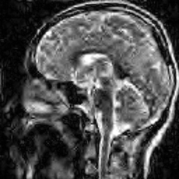
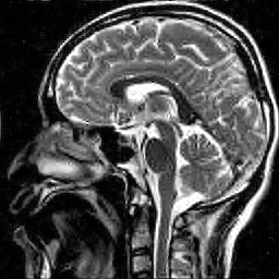
Rand. Gauss to DB4, BCS, err = 29.6%	Multilevel DFT to DB4, $\ell^{1}$, err = 18.2%

Figure 6: Recovery from 12.5% measurements at $256\!\times\!256$. Comparison between random sampling with structured recovery and structured sampling with $\ell^{1}$-minimization recovery.

Structured sparsity within the context of compressed sensing has been considered in numerous previous works. See BaranuikModelCS ; BourrierEtAlInstance ; CalderbankCommInspCS ; donohoCS ; DuarteEldarStructuredCS ; EldarUnionSubspace ; HeCarinStructCS ; HeCarinTreeCS ; EldarXampling2 ; DonohoCSext ; CalderbankNIPS ; TurboAMP and references therein. For the problem of reconstructing wavelet coefficients, most efforts have focused on their inherent tree structure (see Remark 3). Three well-known algorithmic approaches for doing this are model-based compressed sensing BaranuikModelCS , TurboAMP TurboAMP , and Bayesian compressed sensing HeCarinStructCS ; HeCarinTreeCS . All methods use Gaussian or Bernoulli random measurements, and seek to leverage the wavelet tree structure – the former deterministically, the latter two in a probabilistic manner – by appropriately-designed recovery algorithms (based on modifications of existing iterative algorithms for compressed sensing). In other words, structure is incorporated solely in the recovery algorithm, and not in the measurements themselves.

In Figure 6 we compare these algorithms with the previously-described method of multilevel Fourier sampling (similar results are also witnessed with the Hadamard matrix). Note that the latter, unlike other three methods, exploits structure by taking appropriate measurements, and uses an unmodified compressed sensing algorithm ($\ell^{1}$ minimization). As is evident, this approach is able to better exploit the sparsity structure, leading to a significantly improved reconstruction. This experiment is representative of a large set tested. In all cases, we find that exploiting structure by sampling with asymptotically incoherent Fourier/Hadamard bases outperforms such approaches that seek to leverage structure in the recovery algorithm.

6 The Restricted Isometry Property in levels

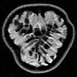
Subsampling pattern	DFT to DB4,	DFT to Levels Flipped DB4,
	error = 10.95%	error = 12.28%

Figure 7: The flip test in levels for the image considered in Figure 1.

The flip test demonstrates that the subsampled Fourier/wavelets matrix $P_{\Omega}U$ does not satisfy a meaningful RIP. However, due to the sparsity structure of the signal, we are still able to reconstruct, as was confirmed in Theorem 4.1. The RIP is therefore too crude a tool to explain the recoverability properties of structured sensing matrices. Having said that, the RIP is a useful for deriving uniform, as opposed to nonuniform, recovery results, and for analyzing other compressed sensing algorithms besides convex optimization, such as greedy methods FoucartRauhutCSbook . This raises the question of whether there are alternatives which are satisfied by such matrices. One possibility which we now discuss is the RIP in levels. Throughout this section we shall work in the finite-dimensional setting. For proofs of the theorems, see Bastounis .

Definition 6

Given an $r$-level sparsity pattern $(\mathbf{k},\mathbf{M})$, where $M_{r}=n$, we say that the matrix $A\in\mathbb{C}^{m\times n}$ satisfies the RIP in levels ($\text{RIP}_{L}$) with $\text{RIP}_{L}$ constant $\delta_{\mathbf{k}}\geq 0$ if for all $x$ in $\Sigma_{\mathbf{k,M}}$ we have

$$(1-\delta_{\mathbf{k}})\|x\|^{2}_{2}\leq\|Ax\|^{2}_{2}\leq(1+\delta_{\mathbf{k}})\|x\|^{2}_{2}.$$

The motivation for this definition is the following. Suppose that we repeat the flip test from Figure 1 except that instead of completely flipping the coefficients we only flip them within levels corresponding to the wavelet scales. We will refer to this as the flip test in levels. Note the difference between Figure 1 and Figure 7, where latter presents the flip test in levels: clearly, flipping within scales does not alter the reconstruction quality. In light of this experiment, we propose the above RIP in levels definition so as to respect the level structure.

We now consider the recovery properties of matrices satisfying the RIP in levels. For this, we define the ratio constant $\lambda_{\mathbf{k,M}}$ of a sparsity pattern $(\mathbf{k},\mathbf{M})$ to be $\lambda_{\mathbf{k,M}}:=\max_{j,l}k_{j}/k_{l}.$ We assume throughout that $k_{j}\geq 1$, $\forall j$, so that $\eta_{\mathbf{k},\mathbf{M}}<\infty$, and also that $M_{r}=n$. We now have the following:

Theorem 6.1

Let $(\mathbf{k},\mathbf{M})$ be a sparsity pattern with $r$ levels and ratio constant $\lambda=\lambda_{\mathbf{k,M}}$. Suppose that the matrix $A$ has $\text{RIP}_{L}$ constant $\delta_{2\mathbf{k}}$ satisfying

$$\delta_{2\mathbf{k}}<\frac{1}{\sqrt{r(\sqrt{\lambda}+1/4)^{2}+1}}.$$ (13)

Let $x\in\mathbb{C}^{n}$, $y\in\mathbb{C}^{m}$ be such that $\|Ux-y\|_{2}\leq\eta$, and let $\hat{x}$ be a minimizer of

$$\min_{z\in\mathbb{C}^{n}}\|z\|_{1}\quad\mbox{s.t.}\quad\|y-Az\|_{2}\leq\eta.$$

Then

$$\|x-\hat{x}\|_{1}\leq C\sigma_{\mathbf{k},\mathbf{M}}(x)_{1}+D\sqrt{k}\eta,$$ (14)

where $k=k_{1}+\ldots+k_{r}$ and the constants $C$ and $D$ depend only on $\delta_{2\mathbf{k}}$.

This theorem is a generalization of a known result in standard (i.e. one-level) compressed sensing. Note that (13) reduces to the well-known estimate $\delta_{2k}\leq 4/\sqrt{41}$ FoucartRauhutCSbook when $r=1$. On the other hand, in the multiple level case the reader may be concerned that the bound ceases to be useful, since the right-hand side of (13) deteriorates with both the number of levels $r$ and the sparsity ratio $\lambda$. As we show in the following two theorems, the dependence on $r$ and $\lambda$ in (13) is sharp:

Theorem 6.2

Fix $a\in\mathbb{N}$. There exists a matrix $A$ with two levels and a sparsity pattern $(\mathbf{k},\mathbf{M})$ such that the $\text{RIP}_{L}$ constant $\delta_{a\mathbf{k}}$ and ratio constant $\lambda=\lambda_{\mathbf{k,M}}$ satisfy

$$\delta_{a\mathbf{k}}\leq 1/|f(\lambda)|,$$ (15)

where $f(\lambda)=o(\sqrt{\lambda})$, but there is an $x\in\Sigma_{\mathbf{k},\mathbf{M}}$ such that $x$ is not the minimizer of

$$\min_{z\in\mathbb{C}^{n}}\|z\|_{1}\quad\mbox{s.t.}\quad Az=Ax.$$

Roughly speaking, Theorem 6.2 says that if we fix the number of levels and try to replace (13) with a condition of the form

$$\delta_{2\mathbf{k}}<\frac{1}{C\sqrt{r}}\lambda^{-\frac{\alpha}{2}}$$

for some constant $C$ and some $\alpha<1$ then the conclusion of Theorem 6.1 ceases to hold. In particular, the requirement on $\delta_{2\mathbf{k}}$ cannot be independent of $\lambda$. The parameter $a$ in the statement of Theorem 6.2 also means that we cannot simply fix the issue by changing $\delta_{2\mathbf{k}}$ to $\delta_{3\mathbf{k}}$, or any further multiple of $\mathbf{k}$.

Similarly, we also have a theorem that shows that the dependence on the number of levels $r$ cannot be ignored.

Theorem 6.3

Fix $a\in\mathbb{N}$. There exists a matrix $A$ and an $r$-level sparsity pattern $(\mathbf{k},\mathbf{M})$ with ratio constant $\lambda_{\mathbf{k,M}}=1$ such that the $\text{RIP}_{L}$ constant $\delta_{a\mathbf{k}}$ satisfies

$$\delta_{a\mathbf{k}}\leq 1/|f(r)|,$$

where $f(r)=o(\sqrt{r})$, but there is an $x\in\Sigma_{\mathbf{k},\mathbf{M}}$ such that $x$ is not the minimizer of

$$\min_{z\in\mathbb{C}^{n}}\|z\|_{1}\quad\mbox{s.t.}\quad Az=Ax.$$

These two theorems suggests that, at the level of generality of the $\text{RIP}_{L}$, one must accept a bound that deteriorates with the number of levels and ratio constant. This begs the question: what is the effect of such deterioration? To understand this, consider the case studied earlier, where the $r$ levels correspond to wavelet scales. For typical images, the ratio constant $\lambda$ grows only very mildly with $n$, where $n=2^{r}$ is the dimension. Conversely, the number of levels is equal to $\log_{2}(n)$. This suggests that estimates for the Fourier/wavelet matrix that ensure an RIP in levels (thus guaranteeing uniform recovery) will involve at least several additional factors of $\log(n)$ beyond what is sufficient for nonuniform recovery (see Theorem 3). Proving such estimates for the Fourier/wavelets matrix is work in progress.

- [1] B. Adcock and A. C. Hansen. Generalized sampling and infinite-dimensional compressed sensing. Technical report NA2011/02, DAMTP, University of Cambridge, 2011.
- [2] B. Adcock, A. C. Hansen, C. Poon, and B. Roman. Breaking the coherence barrier: A new theory for compressed sensing. arXiv:1302.0561, 2014.
- [3] B. Adcock, A. C. Hansen, and B. Roman. A note on compressed sensing of structured sparse wavelet coefficients from subsampled Fourier measurements. arXiv:1403.6541 [math.FA], 2014.
- [4] B. Adcock, A. C. Hansen, B. Roman, and G. Teschke. Generalized sampling: stable reconstructions, inverse problems and compressed sensing over the continuum. Advances in Imaging and Electron Physics (to appear), Elsevier, 2013.
- [5] R. G. Baraniuk, V. Cevher, M. F. Duarte, and C. Hedge. Model-based compressive sensing. IEEE Trans. Inform. Theory, 56(4):1982–2001, 2010.
- [6] A. Bastounis and A. C. Hansen. On the Restricted Isometry Property in Levels. Preprint, 2014.
- [7] P. Binev, W. Dahmen, R. A. DeVore, P. Lamby, D. Savu, and R. Sharpley. Compressed sensing and electron microscopy. In T. Vogt, W. Dahmen, and P. Binev, editors, Modeling Nanoscale Imaging in Electron Microscopy, Nanostructure Science and Technology, pages 73–126. Springer US, 2012.
- [8] A. Bourrier, M. E. Davies, T. Peleg, P. Pérez, and R. Gribonval. Fundamental performance limits for ideal decoders in high-dimensional linear inverse problems. arXiv:1311.6239, 2013.
- [9] E. Candès and D. L. Donoho. Recovering edges in ill-posed inverse problems: optimality of curvelet frames. Ann. Statist., 30(3):784–842, 2002.
- [10] E. J. Candès and D.L. Donoho. New tight frames of curvelets and optimal representations of objects with piecewise singularities. Comm. Pure Appl. Math., 57(2):219–266, 2004.
- [11] E. J. Candès and Y. Plan. A probabilistic and RIPless theory of compressed sensing. IEEE Trans. Inform. Theory, 57(11):7235–7254, 2011.
- [12] E. J. Candès and J. Romberg. Sparsity and incoherence in compressive sampling. Inverse Problems, 23(3):969–985, 2007.
- [13] W. R. Carson, M. Chen, M. R. D. Rodrigues, R. Calderbank, and L. Carin. Communications-inspired projection design with application to compressive sensing. SIAM J. Imaging Sci., 5(4):1185–1212, 2012.
- [14] R. Chartrand, Y. Sidky, and X. Pan. Nonconvex compressive sensing for X-ray CT: an algorithm comparison. In Asilomar Conference on Signals, Systems, and Computers, 2013.
- [15] M. S. Crouse, R. D. Nowak, and R. G. Baraniuk. Wavelet-based statistical signal processing using hidden Markov models. IEEE Trans. Signal Process., 46:886–902, 1998.
- [16] S. Dahlke, G. Kutyniok, G. Steidl, and G. Teschke. Shearlet coorbit spaces and associated Banach frames. Appl. Comput. Harmon. Anal., 27(2):195–214, 2009.
- [17] Stephan Dahlke, Gitta Kutyniok, Peter Maass, Chen Sagiv, Hans-Georg Stark, and Gerd Teschke. The uncertainty principle associated with the continuous shearlet transform. Int. J. Wavelets Multiresolut. Inf. Process., 6(2):157–181, 2008.
- [18] R. A. DeVore. Nonlinear approximation. Acta Numer., 7:51–150, 1998.
- [19] M. N. Do and M. Vetterli. The contourlet transform: An efficient directional multiresolution image representation. IEEE Trans. Image Proc., 14(12):2091–2106, 2005.
- [20] D. L. Donoho. Compressed sensing. IEEE Trans. Inform. Theory, 52(4):1289–1306, 2006.
- [21] M. F. Duarte, M. A. Davenport, D. Takhar, J. Laska, K. Kelly, and R. G. Baraniuk. Single-pixel imaging via compressive sampling. IEEE Signal Process. Mag., 25(2):83–91, 2008.
- [22] M. F. Duarte and Y. C. Eldar. Structured compressed sensing: from theory to applications. IEEE Trans. Signal Process., 59(9):4053–4085, 2011.
- [23] Y. C. Eldar. Robust recovery of signals from a structured union of subspaces. IEEE Trans. Inform. Theory, 55(11):5302–5316, 2009.
- [24] S. Foucart and H. Rauhut. A Mathematical Introduction to Compressive Sensing. Birkhauser, 2013.
- [25] L. Gan, T. T. Do, and T. D. Tran. Fast compressive imaging using scrambled hadamard ensemble. Proc. EUSIPCO, 2008.
- [26] M. Guerquin-Kern, M. Häberlin, K. P. Pruessmann, and M. Unser. A fast wavelet-based reconstruction method for Magnetic Resonance Imaging. IEEE Trans. Med. Imaging, 30(9):1649–1660, 2011.
- [27] M. Guerquin-Kern, L. Lejeune, K. P. Pruessmann, and M. Unser. Realistic analytical phantoms for parallel Magnetic Resonance Imaging. IEEE Trans. Med. Imaging, 31(3):626–636, 2012.
- [28] J. Haldar, D. Hernando, and Z. Liang. Compressed-sensing MRI with random encoding. IEEE Trans. Med. Imaging, 30(4):893–903, 2011.
- [29] L. He and L. Carin. Exploiting structure in wavelet-based Bayesian compressive sensing. IEEE Trans. Signal Process., 57(9):3488–3497, 2009.
- [30] L. He, H. Chen, and L. Carin. Tree-structured compressive sensing with variational Bayesian analysis. IEEE Signal Process. Letters, 17(3):233–236, 2010.
- [31] M. A. Herman and T. Strohmer. High-resolution radar via compressed sensing. IEEE Trans. Signal Process., 57(6):2275–2284, 2009.
- [32] G. Huang, H. Jiang, K. Matthews, and P. Wilford. Lensless imaging by compressive sensing. arXiv:1305.7181, 2013.
- [33] F. Krahmer and R. Ward. Stable and robust recovery from variable density frequency samples. IEEE Trans. Image Proc. (to appear), 2014.
- [34] Gitta Kutyniok, Jakob Lemvig, and Wang-Q Lim. Compactly supported shearlets. In Marian Neamtu and Larry Schumaker, editors, Approximation Theory XIII: San Antonio 2010, volume 13 of Springer Proceedings in Mathematics, pages 163–186. Springer New York, 2012.
- [35] Rowan Leary, Zineb Saghi, Paul A. Midgley, and Daniel J. Holland. Compressed sensing electron tomography. Ultramicroscopy, 131(0):70–91, 2013.
- [36] D. Liang, G. Xu, H. Wang, K. F. King, D. Xu, and L. Ying. Toeplitz random encoding MR imaging using compressed sensing. In Proc. IEEE. Int. Symp. Biomed. Imag., pages 270–273, June 2009.
- [37] T. Lin and F. J. Herrman. Compressed wavefield extrapolation. Geophysics, 72(5):SM77–SM93, 2007.
- [38] M. Lustig, D. L. Donoho, and J. M. Pauly. Sparse MRI: the application of compressed sensing for rapid MRI imaging. Magn. Reson. Imaging, 58(6):1182–1195, 2007.
- [39] M. Lustig, D. L. Donoho, J. M. Santos, and J. M. Pauly. Compressed Sensing MRI. IEEE Signal Process. Mag., 25(2):72–82, March 2008.
- [40] S. G. Mallat. A Wavelet Tour of Signal Processing: The Sparse Way. Academic Press, 3 edition, 2009.
- [41] M. Mishali, Y. C. Eldar, and A. J. Elron. Xampling: Signal acquisition and processing in union of subspaces. IEEE Trans. Signal Process., 59(10):4719–4734, 2011.
- [42] D. D.-Y. Po and M. N. Do. Directional multiscale modeling of images using the contourlet transform. IEEE Trans. Image Proc., 15(6):1610–1620, June 2006.
- [43] G. Puy, J. P. Marques, R. Gruetter, J. Thiran, D. Van De Ville, P. Vandergheynst, and Y. Wiaux. Spread spectrum Magnetic Resonance Imaging. IEEE Trans. Med. Imaging, 31(3):586–598, 2012.
- [44] J. Romberg. Imaging via compressive sampling. IEEE Signal Process. Mag., 25(2):14–20, 2008.
- [45] F. Sebert, Y. M. Xou, and L. Ying. Compressed sensing MRI with random B1 field. Proc. Int. Soc. Magn. Reson. Med, 16:3151, 2008.
- [46] S. Som and P. Schniter. Compressive imaging using approximate message passing and a markov-tree prior. IEEE Trans. Signal Process., 60(7):3439–3448, 2012.
- [47] V. Studer, J. Bobin, M. Chahid, H. Moussavi, E. Candès, and M. Dahan. Compressive fluorescence microscopy for biological and hyperspectral imaging. Submitted, 2011.
- [48] Y. Tsaig and D. L. Donoho. Extensions of compressed sensing. Signal Process., 86(3):549–571, 2006.
- [49] E. van den Berg and M. P. Friedlander. SPGL1: A solver for large-scale sparse reconstruction, June 2007. http://www.cs.ubc.ca/labs/scl/spgl1.
- [50] E. van den Berg and M. P. Friedlander. Probing the pareto frontier for basis pursuit solutions. SIAM J. Sci. Comput., 31(2):890–912, 2008.
- [51] L. Wang, D. Carlson, M. R. D. Rodrigues, D. Wilcox, R. Calderbank, and L. Carin. Designed measurements for vector count data. In Advances in Neural Information Processing Systems, pages 1142–1150, 2013.
- [52] Z. Wang and G. R. Arce. Variable density compressed image sampling. IEEE Trans. Image Proc., 19(1):264–270, 2010.
- [53] Y. Wiaux, L. Jacques, G. Puy, A. M. M. Scaife, and P. Vandergheynst. Compressed sensing imaging techniques for radio interferometry. Mon. Not. R. Astron. Soc., 395(3):1733–1742, 2009.
- [54] E. C. Wong. Efficient randomly encoded data acquisition for compressed sensing. In Proc. Int. Soc. Magn. Reson. Med., page 4893, 2010.