Multi-agent Inverse Reinforcement Learning for Two-person Zero-sum Games
Abstract
The focus of this paper is a Bayesian framework for solving a class of problems termed multi-agent inverse reinforcement learning (MIRL). Compared to the well-known inverse reinforcement learning (IRL) problem, MIRL is formalized in the context of stochastic games, which generalize Markov decision processes to game theoretic scenarios. We establish a theoretical foundation for competitive two-agent zero-sum MIRL problems and propose a Bayesian solution approach in which the generative model is based on an assumption that the two agents follow a minimax bi-policy. Numerical results are presented comparing the Bayesian MIRL method with two existing methods in the context of an abstract soccer game. Investigation centers on relationships between the extent of prior information and the quality of learned rewards. Results suggest that covariance structure is more important than mean value in reward priors.
Index Terms:
Multi-agent Inverse Reinforcement Learning, Zero-sum Stochastic Games, Bayesian Framework.I Introduction
Learning from demonstrations (LD) is a traditional line of research in behavior learning, and is particularly useful in game design. In LD, policy learning directly from observations has achieved remarkable success in large part because it can benefit from advanced supervised learning techniques. Examples of this point can be seen in [1], where preference learning is used for policy learning, and in [2], where a deep convolutional neural network is adopted as the basis for policy learning. In recent years, reinforcement learning (RL) has attracted the interest of game designers because it aligns with the belief that behavior is mainly reward-driven (see, e.g., [3, 4]). Inverse reinforcement learning (IRL), which aims to recover reward (equivalently, payoff or cost) functions given measurements of an agent’s behavior over time as well as a model of the environment, was introduced in [5] and then formalized in [6] in the context of several linear programming algorithms. One can view the IRL problem as being that of learning the reward structure for a game given observations of the play of an expert. One major advantage of IRL, as pointed out in [6], is that in many applications, the reward function provides a parsimonious description of behavior that is succinct, robust, and transferable with respect to changes in the environment. In comparison to policy learning, the benefit of IRL to the game community is that it has the potential to yield insights into the value systems driving player behavior, which in turn might help designers balance the difficulty of the game play and tune the user experience.
One shortcoming of IRL that is particularly relevant to games is that it assumes no other adaptive agents exist in the environment. However, many games are multi-agent, mutually influential systems. To jointly consider the decision making processes of interacting rational agents requires different models and techniques. In the forward direction, multi-agent reinforcement learning (MRL), proposed by Littman [7], extends RL to a multi-agent framework. Littman makes use of stochastic games (see, e.g., [8]) to model MRL, limiting consideration to the special case of two-player zero-sum games, in which one agent’s gain is always the other’s loss, and applies this algorithm in a simple grid-world soccer game. Hu and Wellman [9] extend Littman’s work, proposing a two-player general-sum stochastic game framework for the MRL problem. They point out that the concept of optimality loses its meaning in MRL problems since any agent’s payoff depends on the action choices of others. Consequently, they adopt as a solution concept the Nash equilibrium, in which each agent’s choice is the best response to other agents’ choices. Later MRL work has focused on the development of solution concepts and methods, in competing games as well as cooperative games, including [10, 11, 12, 13]. Representative applications include traffic control [14] and robotics [15].
The inverse learning problem for MRL, or multi-agent inverse reinforcement learning (MIRL), is more complicated than IRL. In the context of a stochastic game being played by two or more agents, the problem is that of estimating the game payoffs given observations of the actions taken by the players and the state transitions. Games bring two primary challenges relative to the Markov decision processes (MDPs) used in IRL. First, as Hu and Wellman [9] note, the concept of optimality, central to MDPs, must be replaced with an equilibrium solution concept, such as the Nash equilibrium. Second, the non-uniqueness of equilibrium strategies (especially for two-player non-zero sum games) means that in MIRL, in addition to multiple reasonable solutions for a given inversion model, theoretically there may be multiple inversion models that are all equally sensible approaches to solving the problem.
This paper proposes a novel Bayesian approach to MIRL. We establish a theoretical foundation for competitive two-agent zero-sum MIRL problems and describe Bayesian MIRL (BMIRL), a Bayesian solution approach in which the generative model is based on an assumption that the two agents follow a minimax bi-policy. To our knowledge, this topic has not been deeply studied in the literature. Natarajan et al. [16] present an inverse reinforcement learning model for multiple agents. However, that paper does not consider competing agents or game-theoretic models, a key characteristic of our work. Waugh et al. [17] do consider a form of the inverse equilibrium problem. However, that paper considers simultaneous one-stage games, rather than the sequential stochastic games we consider here. A similar method, termed decentralized MIRL (d-MIRL), is a decentralized linear IRL approach based off work by Reddy et al. [18], while our work is centralized and set in a Bayesian framework.
Several numerical experiments are performed in the setting of an abstract soccer game with simple grid structure and movement actions and probability models governing ball exchange and the outcomes of ball kicks at the goal (the agents’ shoot action). For the inverse learning problem, the unknown rewards correspond to location of goals and player perception of a successful shot from each position on the field. Investigation centers on relationships between the extent of prior information and the quality of learned rewards. The quality of learned rewards is measured by distance metrics in reward and probability space and by the game playing success of agents that use the rewards as the basis for an equilibrium policy. The weakest priors result in learned rewards that would give an agent using them no chance of winning the game, while the strongest priors result in learned rewards essentially as good as ground truth. Additionally, results suggest that covariance structure is more important than mean value in reward priors.
The remainder of the paper is structured as follows: Section II introduces notation, terminology, definitions, and some basic properties needed for later work. Section III provides the main technical results, including a Bayesian framework for MIRL and formulation of a convex optimization problem for learning rewards. Section IV and V extend the BIRL and d-MIRL approaches to the case where reward is also action dependent. Section VI introduces the soccer model and compares the results generated from the three methods. Section VII provides evaluation of learned rewards of our BMIRL method in terms of game playing success in simulations of the soccer game. Section IX and X offer concluding remarks and a discussion of future work, respectively.
II Preliminaries
II-A Stochastic Games
A two-player discounted stochastic game is played as follows. The game begins in one of finitely many states. There is a reward for each player. In each state, each player simultaneously selects one of finitely many actions, and hence receives a reward that associates with current state and sometimes, as well as the actions selected by one or both players. The game then makes a stochastic transition to a new state, where the transition is dependent on the starting state and the jointly selected actions. This process is repeated over an infinite time horizon, where geometrically discounted rewards are accrued additively.
Under these rules, we can specify an instance of a two-person zero-sum discounted stochastic game in terms of the state space , the action spaces , two reward vectors and of the two agents involved, state transition probabilities , and a reward discount factor . Reward values are assumed to be dependent on state and the actions taken by the two agents. Hence, the dimension of depends on the the size of , and . We will use to denote a scalar; e.g., represents the reward value gained by agent 1 when the two agents take actions and , respectively, in state .
A solution to a stochastic game is a bi-policy, which provides the rules that each player follows when selecting actions at each state. Without loss of generality, a bi-policy can be specified by a collection of conditional probability mass functions and , where player selects action in state with probability . Each is referred to as the strategy played by player in state .
Given that each player can select from among actions, the strategy followed by player in state can be represented by the vector . The si for state is the set of two column vectors that denote the strategies employed by player 1 and player 2 in state ,
In this notation, the bi-policy is defined as the set of all bi-strategies over all states,
II-B Zero-sum Case
A two-player zero-sum discounted stochastic game is a special case of the game defined above for which . The symmetry of rewards between the two players allows to use to denote . Attention is restricted to the zero-sum case throughout the remainder of the paper.
We use to denote the single-stage expected reward value received by agent at state under bi-policy . Then is a column vector with its th component . Define to be
| (1) | ||||
where is a matrix, whose entries are independent of . We can express this relationship in matrix notation as
| (2) |
where is a matrix constructed from bi-policy , whose th row is:
where
and
The concepts of the value function and -function in MDPs have natural analogs in zero sum stochastic games. In particular, let us define the value function to be the bi-policy-dependent, discounted expected sum of rewards of player as a function of the initial state :
| (3) |
where denotes the state of the game at stage and denotes player ’s expected reward under bi-policy at that stage. Note that the superscript can be removed because of the Markov property. denotes the column vector with th component .
In addition, we define player ’s Q-function of state and action pair , under bi-policy , as
| (4) |
Over all states and actions, we can write equation (4) in matrix notation as
| (5) |
where is a matrix with as its elements.
Let denote transition matrix under bi-policy . Specifically, is the matrix with elements
| (6) |
Note that
| (7) | ||||
This equation can be written in matrix notation as
| (8) |
Thus
| (9) |
where is always invertible for since is a transition matrix. The value function can be expressed in terms of the -function as
| (10) |
where is a matrix for agent , whose element is given by . Note that while is a matrix, the introduced in (5) is an vector. We will use this relationship between the Q-function and the value function to define a minimax bi-policy for a stochastic game.
We will assume that rational agents playing two-player zero-sum stochastic games seek a minimax bi-policy. A minimax bi-policy is an equilibrium, in that it has the property that neither player can change the game value in their favor given that the other player holds their policy fixed. To give a precise definition of a minimax bi-policy, we will start by reviewing the notion of a minimax bi-strategy for a static game [19].
First consider a static (single-stage) zero-sum game, where two players simultaneously choose an action and both players receive a reward determined by the joint choice of actions. The minimax theorem states that for every two-person zero-sum game with finitely many actions, there exists a value and a mixed strategy for each player such that
-
•
Given player 2’s strategy, the best expected reward possible for player 1 is .
-
•
Given player 1’s strategy, the best expected reward possible for player 2 is .
As before, the strategies played by both players in a certain state can be expressed in terms of probability mass functions and . Expressing the reward received by player as an matrix , the value of the game for player under a minimax bi-strategy is given by
A pair and that achieves this value is called a minimax bi-strategy. For zero-sum games, a minimax bi-strategy is also a Nash equilibrium.
The concept of a minimax bi-strategy can be extended to two-player discounted stochastic games via the following theorem [20].
Theorem 1 (Shapley’s Theorem).
There exists a bi-policy such that
| (11) |
for all .
A bi-policy that satisfies Theorem 1 is called a minimax bi-policy. For a minimax bi-policy, gives the game value from each initial state . Throughout the following sections it is assumed that agents are observed playing a game according to a minimax bi-policy and that the complete bi-policy is observable. The minimax nature of the bi-policy can then be used to infer the reward structure of the game.
III Bayesian MIRL
We will formulate two-agent MIRL problems in a Bayesian setting. Bayesian methods have been widely adopted for IRL problems [21, 22, 23, 24, 25, 26, 27]. In a Bayesian setting, we assign a prior distribution to the reward functions. This prior distribution encodes the learner’s initial belief about the reward functions before any observations are made.
Given an observed bi-policy, we can generate a point estimate of the reward function from the posterior distribution over reward functions. To construct this point estimate, we must know the likelihood of observing each bi-policy for each given reward function. So, consideration must be given to determining the appropriate likelihood function for the MIRL problem and to the development of optimization models that can be used to generate point estimates of the reward function.
The BMIRL approach we propose is a maximum a posteriori probability (MAP) estimate of reward under a likelihood function that encodes the notion of a minimax equilibrium. Let denote the prior distribution on the reward of agent (recalling that we denote and for zero-sum games). We will discuss the selection of prior distributions further in Section 3.1. Also, let denote the likelihood of observing bi-policy when the true reward is . Hence now our objective is to maximize , the posterior of rewards given an observing bi-policy, as follows,
III-A Prior Distributions on Rewards
In BMIRL, we use prior distributions over reward functions to model our initial uncertainty in the reward. Although any prior may be used, in this paper we prefer Gaussian priors for rewards. Gaussians are a reasonable choice of prior since they provide a straightforward model for representing uncertainty around a nominal choice of reward function, and have the added benefit of leading to analytically tractable inference procedures.
Specifically, we model , where is the mean of and is the covariance matrix. The probability density function of is
| (12) |
III-B Likelihood Function (Unique Minimax bi-policy)
To model the likelihood function , we assume that the bi-policy which the two agents follow is a unique minimax bi-policy given . The likelihood is then a probability mass function given by
| (13) |
III-C MAP Estimation Model
The posterior distribution of rewards for a given observed bi-policy is now
The MAP estimate of rewards is the vector that maximizes . Thus we wish to solve the problem
| maximize: | (14) | |||
| subject to: |
The remainder of this section will be devoted to developing a tractable characterization of the set of feasible . Consider, as a first step, the class of static, single-stage, zero-sum games. In these games, minimax strategies satisfy the conditions of the following theorem [19, 28].
Theorem 2 (Minimax Theorem).
Consider a two-person zero-sum game with payoff matrix . There exists a value , a mixed strategy for player 1, and a mixed strategy for player 2 such that
| (15) | ||||
where is the vector in which every element is . Moreover, and are an equilibrium bi-strategy and is the game value if and only if (15) holds.
This theorem has direct implications for inverse learning problems. Consider a static game as a special case of the MIRL problem, where the goal is to recover a such that the given bi-strategy is a minimax bi-strategy. Hence, the linear constraints (15) give a characterization of the desired constraint set for a two-person zero-sum static game.
We will now extend this approach to a multi-stage stochastic game. Combining Theorem 1 with Theorem 2, a bi-policy is a minimax bi-policy if and only if
| (16) | ||||
for all . The linear inequalities (16) provide conditions that must hold for the -function and value function of a stochastic game if is a minimax bi-policy.
Since our ultimate goal is to estimate the reward function of a stochastic game, we must introduce additional constraints relating the -function and value function to rewards. From (5) and (9), recall that
| (17) | ||||
and from (1), (2) and (10), we can deduce that
| (18) |
Let denote the obtained when is used as player 1’s policy, and player 2 selects action in all states. In this notation, the inequalities (16) can be expressed as
| (19) | ||||
Substituting the expression for into the expression for in (17), we obtain
| (20) | |||||
| (21) |
Finally, letting
| (22) |
the inequalities (19) can be expressed as
| (23) | ||||
Now we can formulate a convex quadratic program equivalent to (14). Recall that we use a Gaussian prior in this paper, so the objective function in (14) is log-concave. To obtain an equivalent convex optimization problem, we will instead minimize . Combining (23) with the negative log-prior objective, the optimization problem (14) can be solved as the following equivalent convex quadratic program:
| minimize: | (24) | |||
| subject to: | ||||
for all and .
The optimization problem (24) is specific to two-person zero-sum MIRL problems, which is a class of problems in which the reward value depends on both state and bi-actions. The equivalent problem for the case where reward values only depend on state is as follows:
| minimize: | |||
| subject to: | |||
for all and .
It is worth discussing the scalability of the optimization problem. When the problem size, , is large, the inversion of the covariance matrix, which is usually sparse, is computationally expensive (). And even if we obtain the inverse of the covariance matrix (which generally will not be sparse), the objective of this problem includes quadratic monomials, which may not fit into memory. One way to tackle this problem is to first compute the Cholesky upper-triangle factorial of , which often is sparse as itself is sparse. Then let and add it to the constraints. Finally, we rewrite our objective as . This reformulation helps avoid the memory issue.
III-D Discussion on Nonunique bi-policies
In the definition of the likelihood function and the convex program (24) we have implicitly assumed that the stochastic game has a unique minimax bi-policy. It is important to note that this assumption need not hold. Indeed for a static two-person zero-sum games there may exist an infinite number of minimax bi-strategies, even though each such game has a unique Nash equilibrium value. In [28], a sufficient condition for the existence of unique bi-strategy for a static matrix game is given: the square game matrix is nonsingular and .
So it is clear we must consider cases where multiple minimax bipolices exist. For ease of expression in doing so, define the following notation:
-
•
: the stochastic game given one agent’s reward vector is .
-
•
: the set of in which the necessary condition (19) is satisfied.
-
•
: a subset of where is a unique minimax bi-policy for .
-
•
: the optimization problem (24) where .
-
•
: a subproblem of (24) constrained by .
We would like to solve the MAP problem for that accounts for the possibility of multiple minimax strategies. Even with a generative notion such as the idea that agents will select among equal-value equilibrium strategies with uniform probability, however, it is difficult to develop a likelihood for this problem because we cannot easily characterize the set of minimax equilibrium strategies as a function of . As a surrogate, one might adopt , but again this problem is difficult to define directly. An alternate approach is to first solve . Let be the optimal solution to this problem. If then is optimal for . If then form , for small random perturbation . With high probability (cf. [29]) and will be nearly optimal for .
III-E Uniqueness of bi-policy
For a static two-person zero-sum games there may exist multiple minimax bi-strategies, even though each such game has a unique Nash equilibrium. In [28], a sufficient condition for the existence of unique bi-strategy for a matrix game is given: the square game matrix is nonsingular and . Note that this is not the necessary condition for the existence of unique minimax bi-strategy. Rudelson and Vershynin [29] show that a perturbation of any fixed square matrix by a random unitary matrix is well invertible with high probability. From these findings, we can come to conclusion that in a real world two-person zero-sum MIRL problem, a unique bi-policy exists with high probability.
IV Linear d-MIRL
In [18], Reddy et al. consider a decentralized version of MIRL, assuming that the reward of any agent in the multi-agent system only depends on state. Here we extend their approach to a two-person zero-sum MIRL problem in which each agent’s reward depends on state and the actions of both agents. As before, let denote player 1’s reward vector.
In [18], the assumption is made that in a multi-agent system all agents reach a Markov Perfect Equilibrium (MPE). This implies that, for all and all ,
In [18], rewards are selected to maximize the difference between the value of the observed policy and those of pure strategies, which is analogous to the classical approach to single-agent IRL given in [6]. For our notation, the equivalent problem for agent 1 is the following linear program:
| maximize: | |||
| subject to: |
where is an adjustable penalty coefficient for having too many non-zero values in the reward vector.
V Bayesian IRL
In this section, we will model the two-person zero-sum multi-agent inverse problem as an IRL problem, by focusing on one agent, which can be called the agent of interest and regarding the other agent as part of the inadaptive environment. We extend the BIRL approach developed in [26], which is only applicable to state-dependent reward recovery, to our case where the reward depends on both state and the action of the agent of interest. Note that the reward we want to recover is instead of , or for all . Although we now turn to the MDP framework, the terminology and notation introduced in Section II will be used here, unless otherwise specified.
In [26], rewards are selected to maximize the posterior of the observed state-action pairs given a reward vector , with the likelihood being if the observed actions are optimal and otherwise for . For our notation, the equivalent problem for agent 1 is the following linear program:
| minimize: | (25) | |||
| subject to: |
for all , where
and where is a sparse matrix constructed from , whose th row is,
and is conceptually similar to , except for being constructed from a pure policy.
In the above formulation, is the mean of the unknown reward vector as a prior, and is its covariance matrix. Note here we use the notation introduced in Section VI-B.
VI Numerical Example
In this section, we illustrate the BMIRL method developed in the previous sections on a two-player stochastic game modeled on soccer, and compare results with those obtained from d-MIRL and IRL. Though styled after soccer abstractions in [7], the game considered here is richer in that it models an action shoot, which is a direct attempt to score through a ball kick.
VI-A Game and Model
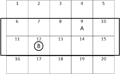
The game is played on a grid as depicted in Figure 1. We use A and B to denote two players, and the circle in the figures to represent the ball. Each player can either stay unmoved or move to one of its neighborhood squares by taking one of 5 actions in each turn: N (north), S (south), E (east), W (west), and stand. If both players land on the same square in the same time period, the ball is exchanged between the two players with some probability. In addition, the player who has the ball can shoot, which is to kick the ball toward their opponent’s goal, with a probability of successful shot (PSS) distribution shown in Table I. A shot can be taken from any field position, and the PSS is independent of opponent’s position. It is worth noting that the PSS at one spot is the probability that the agent believes she would make a successful shot if she kicked the ball at that spot, rather than the actual probability of success she achieves during the play. Otherwise the PSS can be statistically calculated easily through observations once we have inferred the goal area by applying an appropriate MIRL approach.
In the game setting, both players act simultaneously in each time period. Player A attempts to score by reaching with the ball or shooting the ball into squares 6 or 11, and player B attempts to score by reaching with the ball or shooting the ball into squares 10 or 15. Once a point is scored or a shooting is missed, the players take the positions shown in Figure 1 and ball possession is assigned randomly.
As a third-party observer, we have very limited knowledge about the game they play. We know that this is a zero-sum game. We also know that both players aim to score points by taking or kicking the ball to somewhere in the field. Assume that we watch their playing sufficiently long so that we can statistically calculate their complete policies and their ball exchange rate with a perfect accuracy. We will infer which squares each player must reach in order to score a point (the goal squares), as well as the PSS of each player, by means of recovering their reward vector. For example, the PSS of A in position () equals the corresponding reward value because
where is the state where A’s position is . There are in total states in this model, corresponding to the positions of the players and ball possession. Since each player has 6 different actions to choose, each one has a reward vector with a length of . Both players aim to maximize their own total expected points scored, subject to discount factor of .
| PSS = 0.7 | PSS = 0.5 | PSS = 0.3 | PSS = 0.1 | PSS = 0 | |
|---|---|---|---|---|---|
| A | 1, 7, 12, 16 | 2, 8, 13, 17 | 3, 9, 14, 18 | 4, 10, 15, 19 | 5, 20 |
| PSS = 0.7 | PSS = 0.5 | PSS = 0.3 | PSS = 0.1 | PSS = 0 | |
| B | 5, 9, 14, 20 | 4, 8, 13, 19 | 3, 7, 12, 18 | 2, 6, 11, 17 | 1, 16 |
It is worth mentioning that in the simulations done in Section VII the PSS of the two agents happens to be symmetric. As there is some possibility this structure might give rise to confusion with the negative symmetry property of rewards, note that reward symmetry is due to the precondition of zero-sum and is unrelated to the PSS distributions of the agents. The experiments could be performed with arbitrary PSS and ball exchange probabilities.
VI-B Specification of Prior Information
Recall that the MIRL optimization program requires the specification of two Gaussian prior parameters for A, the mean of the rewards vector and the covariance matrix . Below we define a concept of strength for prior information that can be expressed independently in the mean and covariance matrix. Later subsections focus on the impact of different priors on the quality of learned rewards.
VI-B1 Mean of the Prior
We will use three types of mean reward vectors, namely weak mean, median mean and strong mean, respectively. Note that since this is a zero-sum game, the rewards assigned to B are the negatives of these rewards assigned to A.
-
•
Weak Mean: we assign point to player A in every state where A has possession of the ball and point in every state where player B has possession of the ball;
-
•
Median Mean: guessing that A’s goal might be among the rightmost squares, or squares , , and , and symmetrically, B’s goal might be among the leftmost squares, or squares , , and , we assign point to A whenever A has the ball and is in the four leftmost squares, and point to A whenever B has the ball and is in four rightmost squares. Also, when A has the ball and takes a shot, no matter where she is, we assign point to A. Similarly, we assign point to A when B has the ball and takes a shot. Otherwise, no points will be assigned to A.
-
•
Strong Mean: we have a foresight to predict where the goals are for both players, but cannot make a good guess of their PSS distributions. So comparing to median mean, the only difference is that now the potential goal area includes only squares (square and for A and square and for B), rather than squares, for both players.
VI-B2 Covariance Matrix
The covariance matrix of the reward vector encodes our belief of the structure of the prior. Based off of our knowledge of this soccer game, we can develop two types of covariance matrices.
-
•
Weak Covariance Matrix: an identity matrix, indicating that the reward vector is assumed independently distributed. This is a universal covariance matrix suitable for those MIRL problems in which we neither have knowledge of the structure of unknowns, nor want to make a guess.
-
•
Strong Covariance Matrix: a more complex matrix encapsulating some internal information of the reward structure subject to our following beliefs.
-
1.
When A has the ball and takes a shot, the PSS depends only on A’ s position in the field; likewise for B.
-
2.
In any state, the reward for A for any non-shoot action is a state-dependent constant; likewise for B.
-
1.
Note that the strong covariance matrix can be constructed from the correlation matrix, by assuming that the standard deviation of each random variable in the unknown reward vector is the same. In order to avoid singularity, we will add a small perturbation to the diagonal of the covariance matrix.
VI-C Results Evaluation Metric
To evaluate a recovered result, we simply compute its average reward distance (ARD), which is the average Euclidean distance from the true rewards as follows:
| (26) | ||||
where the column vector and denote the recovered and original reward of player . Obviously, the smaller the ARD is, the more accurate the result is.
If only the players’ PSS distributions are of interest, a similar version of the evaluation metric, termed Average PSS Distance (APD) can be defined as
| (27) |
where the column vector and denote the recovered and original PSS of player , respectively.
VI-D Results
Experiments were performed on 6 different priors formed by combining 3 different means and 2 different covariance matrices. A pertubation was used in the construction of the strong covariance matrices. In all cases, the bi-policy followed by the players (the observed input to MIRL) was computed iteratively from Shapley’s Theorem, discussed in Section II-B. Experiments on Bayesian IRL (we can also specify 6 different priors similar to those introduced in Section VI-B) and d-MIRL were also carried out. Note that the reward vector recovered from IRL can be extended to a MIRL reward vector by letting for all .
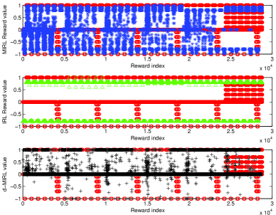
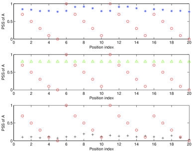
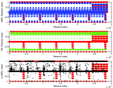
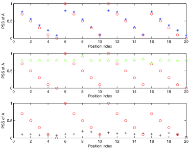
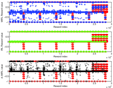
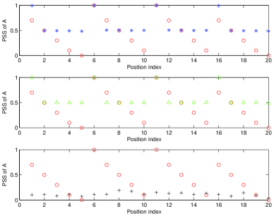
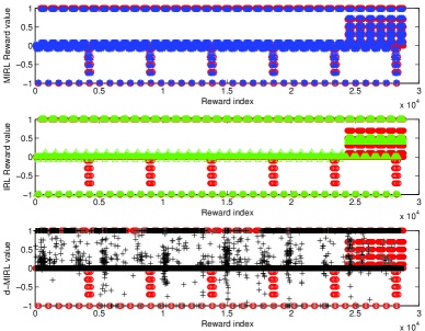
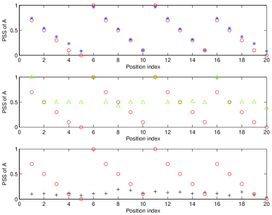
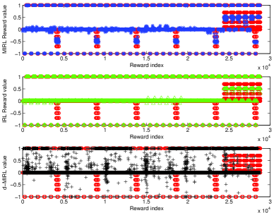
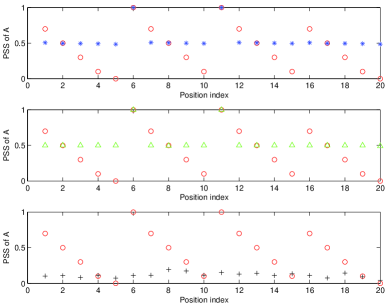
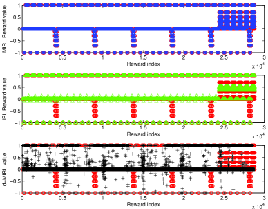
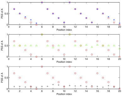
Results are shown in Figures 2-7. Take Figure 3 as an example. Recall that we aim to recover 28800 reward values. In each subfigure in (a), the x-axis represents the reward value index (from 1 to 22800) and the y-axis denotes the reward value. The inferred rewards of BMIRL, BIRL and d-MIRL are shown in blue stars, green triangles and black crosses, respectively, with the benchmark ground truth drawn in red circles in each subfigure. The right three subfigures in (b) show the results of A’s PSSs corresponding to each case. Note that although no shots will be taken at goal positions, for convenience, we set for each player in their goal positions. Table II sorts each experiment with a case number, maps each case to a figure and computes the corresponding APD of the BMIRL rewards.
| Weak Covariance | Strong Covariance | |
|---|---|---|
| Weak Mean | Case 1, Figure 2, 0.4535 | Case 3, Figure 4, 0.0671 |
| Median Mean | Case 3, Figure 4, 0.2169 | Case 4, Figure 5, 0.0387 |
| Strong Mean | Case 5, Figure 6, 0.2058 | Case 6, Figure 7, 0.0259 |
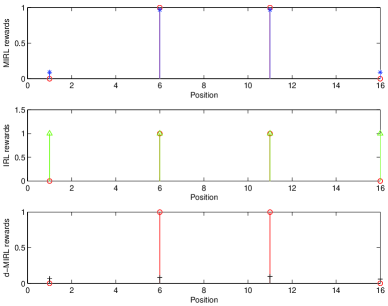
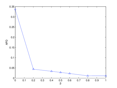
In Case 4, we are also interested in whether the three methods can recover the actual goals for A. We calculate the average reward A receives when A is in square , , and . Results are shown in Figure 9. Now focus on the BMIRL method. It is interesting to consider how the ball exchange rate affects the PSS recovery result. We repeat Case 6 by changing from to , and calculate the APD of the inferred PSS distributions. The result is shown in Figure 9.
VI-E Analysis of Results
From Figures 2-7 and Table II, we can easily come to a conclusion that generally, among the three methods, BMIRL performs much better than the other two. For BMIRL,
-
•
The closer the mean is to the actual rewards, the better the quality of learned rewards will be, and likewise for the covariance matrix.
-
•
The covariance matrix has a greater influence on the quality of learned than does the mean.
From Figure 9 we see that BMIRL successfully learns the goals for A, while the other two methods fail to do so. Finally, Figure 9 shows that the smaller the is, the less accurate the recovered PSS will be. The reason is that players are inclined to dribble the ball rather than shoot it toward their opponents’ goal when is small, and consequently, observing the strategy of dribbling will not generate constraints that substantially alter the mode of the priors on shooting rewards. For example, when , the probability of successfully dribbling the ball to the destination for each player is, at worst, , which means that a shot will never be taken in positions where the agent’s PSS is 0.3 or 0.1.
VII Monte Carlo Simulation using Recovered Rewards
In the previous section, distance metrics in reward and PSS space are used to evaluate the quality of learned rewards. In this section we measure the reward quality in terms of the quality of the forward solution that would be based on the rewards. IRL is often set in the context of apprenticeship learning, in which learned rewards form the basis for anticipating or mimicking the response of agents to unknown situations. In MIRL, the analogous notion is to use learned rewards as the basis for game play in different environmental settings. In this section, we will simulate a series of games, by letting different agents use different rewards generated from the three methods discussed above and play against each other. Being rational, all agents will employ a minimax policy based off of which is the rewards they learned. Specifically, define the following agents:
-
•
A, which uses true rewards;
-
•
B, which uses BMIRL rewards;
-
•
C, which uses BIRL rewards;
-
•
D, which uses d-MIRL rewards.
A full set of agent-to-agent competition then includes the following scenarios:
-
•
B against A;
-
•
B against C;
-
•
B against D.
All those games are simulated in three different environment settings, where the the ball exchange rates are , and , respectively. Note that the symmetry of PSS values means that the two agents are equally skillful and are supposed to be an equal in match both of them follow reasonable policies generated from learned rewards.
The simulation results are presented in Table III-V. In each table, the first column is the different sets of BMIRL rewards that B employs to develop her minimax policy, where WM, MM, SM, WC and SC stand for weak mean, median mean, strong mean, weak covariance matrix and strong covariance matrix, respectively. The remaining columns are the win or lose (W/L) outcomes of 10000 rounds of games between B and other agents in cases where being , and . For example, in Table III, 24.69/25.10 means B beats A with probability 24.69% and loses with probability 25.10%. It indicates that the remaining 50.21% rounds end in a tie. A tie occurs when neither player scores a point. For a more clear comparison, we only count those game episodes ending in win-lose outcomes. Each column except for the first presents B’s winning percentage. Note that in Table IV, since there are also 6 sets of BIRL rewards, comparisons are between corresponding sets, e.g., SM-SC BMIRL vs SM-SC BIRL.
| Base Rewards | W/L% () | W/L% () | W/L% () |
|---|---|---|---|
| WM & WC | 0/24.80 | 0/62.53 | 0/50.30 |
| WM & SC | 24.69/25.10 | 25.10/25.30 | 50.66/49.34 |
| MM & WC | 15.28/25.34 | 14.36/24.69 | 28.44/49.43 |
| MM & SC | 24.73/25.03 | 24.12/25.18 | 49.84/50.16 |
| SM & WC | 14.85/24.52 | 14.94/25.50 | 49.31/50.69 |
| SM & SC | 24.77/25.32 | 24.55/25.43 | 49.84/50.16 |
| Base Rewards | W/L% () | W/L% () | W/L% () |
|---|---|---|---|
| WM & WC | 0/0 | 13.50/0 | 0/0 |
| WM & SC | 23.36/0 | 24.64/0 | 50.29/0 |
| MM & WC | 13.55/0 | 15.64/0 | 26.82/0 |
| MM & SC | 22.73/6.74 | 25.45/14.80 | 49.55/27.58 |
| SM & WC | 15.82/0 | 14.27/0 | 49.87/0 |
| SM & SC | 23.36/0 | 24.64/0 | 50.13/0 |
| Base Rewards | W/L% () | W/L% () | W/L% () |
|---|---|---|---|
| WM & WC | 0/0 | 0/0 | 0/0 |
| WM & SC | 25.52/0 | 26.36/0 | 49.98/0 |
| MM & WC | 12.52/0 | 16.75/0 | 50.26/0 |
| MM & SC | 24.60/0 | 27.30/0 | 49.20/0 |
| SM & WC | 12.24/0 | 13.26/0 | 49.46/0 |
| SM & SC | 25.22/0 | 26.48/0 | 49.90/0 |
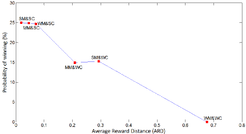
Let us coin the term Application Metric (AM) to refer to B’s probability of winning in the soccer example. Table III shows that A outperforms or ties B in general. This result is reasonable because A uses true rewards. In addition, we compare AM with the previous numerical metric ARD in Figure 10. As expected, a larger ARD results in a smaller probability of winning. What is notable is the sudden crash in probability of winning experienced when ARD becomes sufficiently large. Equivalently, the probability of B’s winning drops sharply when both the mean and covariance are weak. The implication is that inferring the structure of the unknowns, is much more crucial than inferring their true values. As for the other two methods, Tables IV-V show that B generally outperforms C or D.
VIII Additional Experiments
Thus far we have demonstrated the performance of our BMIRL algorithm through a numerical experiment. There remain, however, two important questions to address. First, how does our BMIRL approach compare to supervised/semi-supervised learning based policy learning approaches? Second, can we still expect good performance if the game is played on a larger size grid, say, ?
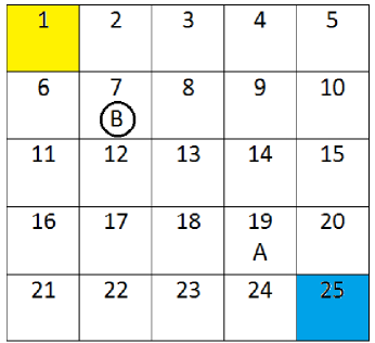
This section is dedicated to addressing these two questions through two more experiments in the context of the soccer game. The first experiment is to use multivariate linear regression to learn a linear relationship between predictors (state and the ball exchange rate) and the response (bi-strategies) and then to infer the response in a new environment. Note that normalization is needed before applying the regression. The second experiment is to re-design the game on a grid, as shown in Figure 11, where A and B’s starting positions are 19 and 7, and their goals are 1 and 25, respectively. The PSS distributions are also re-assigned. Other settings and rules of this new game remain as they are in the old one.
Performance evaluations in these two experiments are conducted through Monte-Carlo simulation as in Section VII. Specifically, in the first experiment, we define agent as using policy-learning method and simulate the scenario of against . In the second experiment, we investigate against , where and denote agents using BMIRL rewards and true rewards in the new game, respectively.
The results of the first experiment, presented in Table VI, show that BMIRL generally outperforms the policy-learning method when a strong covariance matrix is applied in the prior, and generates comparable results with those of the policy-learning method in other cases with the exception of the worst prior condition. In the second experiment, we offer more combinations of mean and covariance as prior information is very critical in the performance of BMIRL. Specifically, we provide one more median covariance matrix, denoted as MC, subject to our beliefs that: (1) when A has the ball and takes a shot, the PSS depends only on A’ s position in the field; and (2) the reward for A for any non-shoot action is generally strongly correlated. As shown in Table VII, results are similar to those from the experiments reported in Table III and confirm the associated conclusions.
| Base Rewards | W/L% () | W/L% () | W/L% () |
|---|---|---|---|
| WM & WC | 0/14.91 | 0/21.30 | 0/36.40 |
| WM & SC | 22.54/21.16 | 19.19/18.11 | 47.15/36.45 |
| MM & WC | 20.82/23.38 | 19.70/17.90 | 40.65/36.85 |
| MM & SC | 28.89/24.46 | 27.98/16.86 | 49.48/40.08 |
| SM & WC | 19.79/23.61 | 19.52/17.88 | 50.15/35.65 |
| SM & SC | 29.04/23.56 | 30.94/20.76 | 50.26/35.44 |
| Base Rewards | W/L% () | W/L% () | W/L% () |
|---|---|---|---|
| WM & WC | 20.20/20.60 | 5.07/4.93 | 25.42/49.78 |
| WM & MC | 20.90/21.20 | 4.44/4.46 | 24.46/50.34 |
| WM & SC | 20.12/21.19 | 24.89/25.80 | 43.60/50.24 |
| MM & WC | 19.41/18.79 | 4.17/4.23 | 24.19/49.11 |
| MM & MC | 20.94/20.86 | 5.32/5.28 | 25.56/49.94 |
| MM & SC | 21.02/20.60 | 24.27/24.62 | 43.60/49.98 |
| SM & WC | 20.02/20.88 | 5.23/5.27 | 25.06/51.34 |
| SM & MC | 20.03/20.07 | 4.23/4.37 | 26.14/51.06 |
| SM & SC | 24.81/25.78 | 25.32/24.72 | 49.84/50.16 |
IX Conclusions
This paper introduces the MIRL problem in the setting of zero-sum stochastic games and presents a solution based on Bayesian inference. Although it seems that MIRL is a natural extension of IRL, it in fact presents more challenges. Even in simple static games two important distinctions between inverse learning for optimization and inverse learning for games emerge. While the model in this paper assumes that the complete bi-policy of two players is observed, it is more likely that only actions of the individual players are observed. In an optimization setting, since deterministic policies are assumed, strategies can be inferred exactly from finitely many observations of actions. In the case of games, strategies are often mixed, and so strategies cannot be inferred exactly from finitely many observations of the actions taken in each state. Therefore, we cannot model a player’s strategy as an observation as it can be done in IRL. In the setting of games, strategies must be treated as latent variables that are not observed directly, but bridge the gap between reward functions and observable actions.
Though ideally structured, the numerical examples considered in this section serve to demonstrate the ill-specified nature of the MIRL problem. Neither BIRL nor d-MIRL perform satisfactorily on the numerical examples. The rationale underlying this phenomenon is that there always exist multiple feasible solutions that are consistent with the observations. It is extremely difficult to select a reward function that is closest to the ground truth without a certain amount of domain knowledge. Our proposed BMIRL approach makes use of domain knowledge expressed as priors on the reward function. That distinction, new to the literature of MIRL methods, is why our Bayesian method is superior to the d-MIRL method in the numerical examples. Fortunately, in many real problems domain knowledge would be available to observers.
A principal motivation for the study of MIRL in game settings is that the approach offers insight into how agents will behave if the game environment, rules, or dynamics change. Such insight may be useful in game design and management, such as balance adjustment. Effective supervised methods exist for learning policies from observed actions, but policies learned in this fashion do not project into new game environments. The reason is that the optimal policy often changes with environment and hence learning from an old policy may not help to infer a new policy. To see this, consider the abstract soccer game. In Section VII, three additional agents B, C and D come up with their own minimax policies by using rewards learned from three different methods, and compete with A in three different environmental settings: the ball exchange rate and . Recall that rewards were learned when . The similarity of two policies, say and , can be measured using the Frobenius distance , defined as: . Table VIII shows the similarity of player B’s policies as a function of . The conclusion to be drawn is that as the environment changes, so does the policy.
| 5.71 | 8.53 | 20.49 |
X Future Work
Several directions are suggested for future work. First, generative models are needed for more general scenarios, such as those where a full bi-policy is unobservable. Such scenarios have been discussed in [18], under the assumption that the agents have reached a minimax equilibrium. There is room for methods that can incorporate domain knowledge and informative priors. Second, an extension of our method to those MIRL problems where the state transition matrix is difficult to obtain or estimate is needed. The approach in this paper requires the state transition matrix to be known. It is well known, however, that RL problems can be addressed without knowing the state transition matrix, and this is true for IRL as well [30]. An extension of MIRL to such setting may be worthwhile. Third, an extension is needed to the -player, general-sum case. This will likely be challenging, because in general-sum games, multiple equilibria may be associated with different game values. Moreover, the specific assumptions imposed on equilibrium selection will affect the nature of the reward functions recovered from an inverse learning procedure. A good starting point for study of general sum games would be multi-player, stochastic iterated Prisoners’ Dilemma, as the MIRL perspective might allow the interpretation of learned rewards in terms of the dynamics of strategy evolution.
Acknowledgment
This work was partially supported by Science Applications International Corporation (SAIC) through the Research Scholars Fellowship Program.
References
- [1] T. R. Runarsson and S. M. Lucas, “Preference learning for move prediction and evaluation function approximation in Othello,” IEEE Transactions on Computational Intelligence and AI in Games, vol. 6, no. 3, pp. 300–313, 2014.
- [2] C. J. Maddison, A. Huang, I. Sutskever, and D. Silver, “Move evaluation in go using deep convolutional neural networks,” in Proceedings of the International Conference on Representation Learning (ICLR’15), 2015.
- [3] H. Wang, Y. Gao, and X. Chen, “Rl-dot: A reinforcement learning npc team for playing domination games,” IEEE Transactions on Computational Intelligence and AI in Games, vol. 2, no. 1, pp. 17–26, 2010.
- [4] F. G. Glavin and M. G. Madden, “Adaptive shooting for bots in first person shooter games using reinforcement learning,” IEEE Transactions on Computational Intelligence and AI in Games, vol. 7, no. 2, pp. 180–192, 2015.
- [5] S. Russell, “Learning agents for uncertain environments (extended abstract),” in Proc. Ann. Conf. on Comp. Learning Theory (COLT’98), 1998, pp. 101–103.
- [6] A. Y. Ng and S. Russell, “Algorithms for inverse reinforcement learning,” in Proc. Intl. Conf. Mach. Learning (ICML’00), 2000, pp. 663–670.
- [7] M. L. Littman, “Markov games as a framework for multi-agent reinforcement learning,” in Proc. Intl. Conf. Mach. Learning (ICML’94), 1994, pp. 157–163.
- [8] G. Owen, Game Theory, 1st ed. Philadelphia, PA: W. B. Saunders Company, 1968.
- [9] J. Hu and M. P. Wellman, “Multiagent reinforcement learning: Theoretical framework and an algorithm,” in Proc. Intl. Conf. on Mach. Learning (ICML’98), 1998, pp. 242–250.
- [10] S. Abdallah and V. Lesser, “A multiagent reinforcement learning algorithm with non-linear dynamics,” J. Artif. Intell. Res., vol. 33, pp. 521–549, 2008.
- [11] M. Ghavamzadeh, S. Mahadevan, and R. Makar, “Hierarchical multi-agent reinforcement learning,” Autonom. Agents Multi-Agent Syst., vol. 13, pp. 197–229, 2006.
- [12] S. D. Patek, P. A. Beling, and Y. Zhao, “Natural solutions for a class of symmetric games,” in AAAI Spring Symp. Game Theoretic Decision Theoretic Agents, 2007, pp. 47–53.
- [13] Y. Zhao, S. Patek, and P. Beling, “Decentralized bayesian search using approximate dynamic programming methods,” IEEE Trans. Syst., Man, Cybern. B, vol. 38, no. 4, pp. 970–975, 2008.
- [14] A. L. C. Bazzan, “Opportunities for multiagent systems and multiagent reinforcement learning in traffic control,” Autonom. Agents Multi-Agent Syst., vol. 18, pp. 342–375, 2009.
- [15] Y. Duan, B. X. Cui, and X. Xu, “A multi-agent reinforcement learning approach to robot soccer,” Artificial Intelligence Review, vol. 38, no. 3, pp. 193–211, 2012.
- [16] S. Natarajan, G. Kunapuli, K. Judah, P. Tadepalli, K. Kersting, and J. W. Shavlik, “Multi-agent inverse reinforcement learning,” in Proc. Intl. Conf. Mach. Learning App. (ICMLA’10), 2010, pp. 395–400.
- [17] K. Waugh, B. Ziebart, and J. Bagnell, “Computational rationalization: The inverse equilibrium problem,” in Proc. Intl. Conf. Mach. Learning (ICML’11), 2011, pp. 1169–1176.
- [18] T. S. Reddy, V. Gopikrishna, G. Zaruba, and M. Huber, “Inverse reinforcement learning for decentralized non-cooperative multiagent systems,” in Proc. IEEE Intl. Conf. Syst., Man, Cybern. (SMC’12), 2012.
- [19] J. Neumann and O. Morgenstern, Theory of Games and Economic Behavior. Princeton, NJ: Princeton University Press, 1944.
- [20] L. S. Shapley, “Stochastic games,” Proc. Nat. Academy Sci., Math., vol. 39, pp. 1095–1100, 1953.
- [21] C. L. Baker, R. Saxe, and J. B. Tenenbaum, “Action understanding as inverse planning,” Cognition, vol. 113, no. 3, pp. 329–349, 2009.
- [22] J. Choi and K. Kim, “Map inference for bayesian inverse reinforcement learning,” in Proc. Adv. Neural Info. Proc. Syst. (NIPS’01), 2011, pp. 1989–1997.
- [23] C. Dimitrakakis and C. A. Rothkopf, “Bayesian multitask inverse reinforcement learning,” in Proc. Euro. Workshops Reinforcement Learning (EWRL’11), 2011, pp. 273–284.
- [24] Y. Engel, S. Mannor, and R. Meir, “Reinforcement learning with gaussian processes,” in Proc. Intl. Conf. Mach. learning (ICML’05), 2005, pp. 201–208.
- [25] B. Michini and J. P. How, “Bayesian nonparametric inverse reinforcement learning,” in Proc. Euro. Conf. Mach. Learning, Principles, Practice of Knowledge Discov. in Databases (ECML/PKDD’12), vol. 2, 2012, pp. 148–163.
- [26] Q. Qiao and P. A. Beling, “Inverse reinforcement learning with gaussian process,” in Proc. American Control Conf. (ACC’11), 2011, pp. 113 –118.
- [27] D. Ramachandran and E. Amir, “Bayesian inverse reinforcement learning,” in Proc. Intl. Joint Conf. Artif. Intell. (IJCAI’07), 2007, pp. 2586–2591.
- [28] T. S. Ferguson, Game Theory. UCLA, 2008.
- [29] M. Rudelson and R. Vershynin, “Invertibility of random matrices: Unitary and orthogonal perturbations,” J. American Math. Soci., vol. 27, pp. 293–338, 2014.
- [30] S. Levine, Z. Popović, and V. Koltun, “Nonlinear inverse reinforcement learning with gaussian processes,” in Proc. Adv. in Neural Info. Proc. (NIPS’11), 2011, pp. 19–27.