Singularities in Large Deviation Functionals of Bulk-Driven Transport Models

Abstract

The large deviation functional of the density field in the weakly asymmetric simple exclusion process with open boundaries is studied using a combination of numerical and analytical methods. For appropriate boundary conditions and bulk drives the functional becomes non-differentiable. This happens at configurations where instead of a single history, several distinct histories of equal weight dominate their dynamical evolution. As we show, the structure of the singularities can be rather rich. We identify numerically analogues in configuration space of first order phase transition lines ending at a critical point and analogues of tricritical points. First order lines terminating at a critical point appear when there are configurations whose dynamical evolution is controlled by two distinct histories with equal weight. Tricritical point analogues emerge when there are configurations whose dynamical evolution is controlled by three distinct histories with equal weight. A numerical analysis suggests that the structure of the singularities can be described by a Landau like theory. Finally, in the limit of an infinite bulk bias we identify singularities which arise from a competition of $s$ histories, with $s$ arbitrary. In this case we show that all the singularities can be described by a Landau like theory.

Keywords: Out of Equilibrium Statistical Mechanics, Driven Diffusive Systems, Large Deviation Functional, Phase Transitions

1 Introduction

In recent years there has been much focus on understanding full probability distributions in non-equilibrium systems. In particular, much progress has been achieved in the context of driven diffusive systems [1]. For these systems there is a growing understanding of both probability distributions of currents [2, 3, 4, 5, 6, 7, 8, 9] and density profiles [10, 11, 12, 13, 14, 15, 16, 17]. In the latter case, which is the focus of this paper, it can be shown that for a large class of systems the probability distribution of a density field $\rho({\bf x})$ obeys a large deviation principle [18, 19]:

$$P\left[\rho({\bf x})\right]\sim e^{-N\phi\left[\rho({\bf x})\right]}\;.$$ (1)

Here ${\bf x}$ is a spatial coordinate, $N$ is the system size, $P\left[\rho({\bf x})\right]$ is the probability functional of the density field and $\phi\left[\rho({\bf x})\right]$ is the large deviation functional (LDF). In equilibrium $\phi\left[\rho({\bf x})\right]$ is given by the free energy of the system. Therefore, out of equilibrium it can be considered as a direct analogue of the free energy.

In equilibrium, when the system is a diffusive gas in a disordered phase and the interactions are short ranged $\phi\left[\rho({\bf x})\right]$ is a local and smooth functional. By smooth it is meant that as $\rho({\bf x})$ is varied smoothly the functional $\phi\left[\rho({\bf x})\right]$ changes continuously. By now it is understood that out of equilibrium these properties change in a rather dramatic manner. In general, when the field $\rho({\bf x})$ is conserved in the bulk of the system, $\phi\left[\rho({\bf x})\right]$ becomes a non-local functional [20, 11]. This is directly related to the long-range correlations which are known to exist in such systems for many years [20, 21, 22, 23]. Moreover, more recently it was realized that the functional can be non-differentiable [14, 24, 25]. Namely, for given configurations derivatives of $\phi\left[\rho({\bf x})\right]$ change discontinuously as $\rho(x)$ is varied. Such singularities are well understood for many years in the context of low dimensional systems [26, 27, 28, 29, 30] and it is of interest to see 1) when they appear in continuum infinite dimensional systems and 2) how they can be characterized. By now it has been shown that the singularities occur for the weakly driven asymmetric simple exclusion process (WASEP) in the limit of large bulk driving field [14] and for a class of boundary driven diffusive systems [24, 25]. In the latter case, the singularities that were uncovered so far are of a rather simple form that can be described by a mean-field Ising like singularity (or in terms of catastrophe theory as a cusp singularity). It was also shown that in the limit of small bulk bias the functional becomes smooth as expected from the known results for the symmetric simple exclusion process (SSEP). However, it is unclear which singularities appear or how they can be described.

In this paper we take a closer look at singularities in the LDF of the WASEP. As mentioned above the existence of singularities was first shown in [14]. Specifically, the work proved the existence of first order like singularities in the limit of a large bulk driving field. However, the structure of the singularities was not studied. Here, building on the results of [14], we extend the study of singularities in the WASEP significantly using a combination of numerical and analytical results. We first show, numerically, how the singularities appear as the bulk bias is increased. It is shown that for small bulk bias simple cusp like (or mean-field Ising like) singularities appear. However, as the bulk bias increases the structure of the singularities becomes more complicated and we identify numerically an analogue of a tricritical point, also known as a symmetry-restricted butterfly catastrophe [31]. For the cusp singularity we give evidence that it can be described using a simple Landau like theory with an Ising symmetry, along the lines of [25]. For the tricritical point the numerics are not precise enough to verify that it can be described by a Landau theory. We then consider the limit of an infinite bulk drive, namely, the partially asymmetric simple exclusion process (PASEP) in the hydrodynamic limit [32] (For an exact definition see the discussion below). We characterize the singularity found in [14] to show that the first order like singularity found there is a consequence of a cusp singularity and extend the result to further show that analogues of multicritical points of any order appear. Finally we show that in these can all be described using a Landau like theory.

The structure of the paper is as follows. In section 2 we describe the WASEP and PASEP models in the hydrodynamic limit. In section 3 we describe the Macroscopic Fluctuation Theory and the solution obtained for the WASEP in [14]. The numerical results for the singularities in the WASEP in the weak bulk bias case are described in section 4. In section 5 we present analytical results for the PASEP, including a mapping of the LDF of specific configurations to Landau theory of multicritical points.

2 The Model

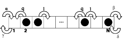
Figure 1: A pictorial illustration of the WASEP and PASEP. Particles hope to the right (left) with rate $1$ ($q$), provided that the site is empty. At the left (right) boundary particles are injected with rate $\alpha$ ($\delta$) and removed with rate $\gamma$ ($\beta$).

We consider the WASEP on a one-dimensional lattice with $N$ sites (see Fig. 1). Particles hop to the left with rate $q$ and to the right with rate $1$ (in arbitrary time units), as long as the site that they hop to is not occupied. At the left boundary, a particle is injected to site 1 with rate $\alpha$ (as long as site 1 is vacant), and if there is a particle at site 1, it is removed with rate $\gamma$. Similarly, at the right boundary, a particle is injected to site $N$ with rate $\delta$, and removed with rate $\beta$. When $q=1$, the bulk diffusion is unbiased, and the process reduces to a SSEP.

The WASEP is defined in the limit when $1-q\sim N^{-1}$, meaning that the bias strength scales inversely with system size. For this case, in the hydrodynamic limit, the equation of motion for the particle density field is [33]

$$\partial_{t}\rho\left(x,t\right)+\partial_{x}J\left(x,t\right)=0,$$ (2)

with

$$J\left(x,t\right)=-\frac{1}{2}\partial_{x}\rho\left(x,t\right)+\sigma\left(\rho\right)E+\sqrt{\sigma\left(\rho\right)}\eta\left(x,t\right).$$ (3)

Here the spatial coordinate is rescaled by $N^{-1}$ and time by $N^{-2}$, the diffusion coefficient has been set to $\nicefrac{{1}}{{2}}$ (in appropriate units), $E$ is the bulk drive (proportional to $1-q$), and $\eta\left(x,t\right)$ is an uncorrelated white noise which satisfies $\left\langle\eta\left(x,t\right)\right\rangle=0$ and $\left\langle\eta\left(x,t\right)\eta\left(x^{\prime},t^{\prime}\right)\right\rangle=N^{-1}\delta\left(t-t^{\prime}\right)\delta\left(x-x^{\prime}\right)$, with $N$ the system size. The dependence of the noise on $N$ is a direct result of the rescaling of distances in the system. The noise amplitude is given by $\sigma\left(\rho\right)=\rho\left(1-\rho\right)$ so that locally the equations of motion satisfy the fluctuation-dissipation relation $\sigma(\rho)=k_{B}T\rho^{2}\kappa(\rho)$, where $\kappa(\rho)$ is the compressibility of a gas of diffusing hardcore particles, $T$ is the temperature and $k_{B}$ is the Boltzmann constant. The system is attached to two reservoirs at $x=0$ and $x=1$ which impose the boundary conditions

$$\rho(x=0)=\rho_{0}=\frac{\alpha}{\alpha+\gamma}\quad;\quad\rho(x=1)=\rho_{1}=\frac{\delta}{\delta+\beta}\ .$$

Throughout the paper our interest is in the case $\rho_{0}<\rho_{1}$ and $E>0$. Namely, the boundary conditions promote a particle current in the negative $x$ direction and the field $E$ promotes a particle current in the positive $x$ direction. The average density profile $\bar{\rho}\left(x\right)$, which is also the most probable one, is obtained by solving $-\frac{1}{2}\partial_{x}^{2}\bar{\rho}+\partial_{x}\sigma\left(\bar{\rho}\right)E=0$ with the boundary conditions $\rho_{0}$ and $\rho_{1}$. Fig. 2 shows that as $E$ increases it changes from a linear density profile ($E=0$) to a step-like structure whose width scales, by dimensional analysis, as $1/E$ (with the diffusion coefficient set to be $\nicefrac{{1}}{{2}}$). In the limit $E\to\infty$ one reproduces the steady-state obtained for the PASEP using a matrix product ansatz [34, 35]. Note that in the general the system is out of equilibrium, except for the specific choice $E=\log\frac{\rho_{1}}{1-\rho_{1}}-\log\frac{\rho_{0}}{1-\rho_{0}}$, for which that system is in equilibrium. In this case the average current is equal to zero throughout the system.

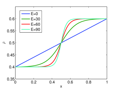
Figure 2: Steady states of the WASEP for different values of $E$. The boundary conditions are $\rho_{0}=0.4,\,\rho_{1}=0.6$. As $E$ increases, the slope of the density profile in the middle of the interval becomes steeper.

To study the probabilities of large deviations for such a system we use the macroscopic fluctuation theory (MFT) [36, 37]. It will also be important for describing the structure and occurrence of singularities in the LDF. To this end, in the next section we outline the MFT for the WASEP, building on [14].

3 Macroscopic Fluctuation Theory

For our purpose it is most convenient to use a Hamiltonian approach. To this end, we use a standard Martin-Siggia-Rose formalism [38]. Since we are interested in the steady-state probability density we evaluate the probability of observing a certain density profile $\rho_{f}$ at time $t=0$, given that the system was at $\bar{\rho}$ at $t\rightarrow-\infty$. This is given by

$$P\left[\rho_{f}\left(x\right)\right]\sim\int\mathcal{D}\rho\mathcal{D}\eta\,\delta\left(\partial_{t}\rho+\partial_{x}J\right)\exp\left[-N\int_{-\infty}^{0}\mathrm{d}\tau\int_{0}^{1}\mathrm{d}x\frac{\eta^{2}}{2}\right],$$ (4)

with the boundary conditions $\rho(x=0,t)=\rho_{0}$, $\rho(x=1,t)=\rho_{1}$, $\rho(x,t=-\infty)=\overline{\rho}(x)$ and $\rho(x,t=0)=\rho_{f}(x)$. Then following the standard procedure we introduce an auxiliary field $\hat{\rho}$ and integrate over the noise to obtain

$$P\left[\rho_{f}\left(x\right)\right]\sim\int\mathcal{D}\rho\mathcal{D}\hat{\rho}\,\exp\left[-N\int_{-\infty}^{0}\mathrm{d}\tau\int_{0}^{1}\mathrm{d}x\left(\hat{\rho}\partial_{t}\rho+\frac{1}{2}\partial_{x}\hat{\rho}\partial_{x}\rho-\partial_{x}\hat{\rho}\sigma\left(\rho\right)E-\frac{1}{2}\left(\partial_{x}\hat{\rho}\right)^{2}\sigma\left(\rho\right)\right)\right].$$ (5)

As a result of boundary densities being fixed the field $\hat{\rho}$ satisfies the boundary conditions $\hat{\rho}(x=0)=0$ and $\hat{\rho}(x=1)=0$ [39].

In the large $N$ limit, which is of interest in this work, one evaluates the path-integral using a saddle-point approximation. This yields histories from the most probable configuration $\bar{\rho}\left(x\right)$ at $t=-\infty$ to $\rho_{f}(x)$ at $t=0$ which satisfy the Hamilton equations

$$\partial_{t}\rho+\partial_{x}\sigma\left(\rho\right)E = \frac{1}{2}\partial_{x}^{2}\rho-2\partial_{x}\left(\sigma\left(\rho\right)\partial_{x}\hat{\rho}\right)$$ (6)

$$\partial_{t}\hat{\rho}+E\partial_{x}\sigma\left(\rho\right)\partial_{x}\hat{\rho} = -\left(\partial_{x}\hat{\rho}\right)^{2}\cdot\partial_{x}\sigma\left(\rho\right)-\frac{1}{2}\partial_{x}^{2}\hat{\rho}\;.$$ (7)

The LDF is then given by

$$\phi[\rho_{f}(x)]=\inf_{i}\phi_{i}[\rho_{f}(x)]$$ (8)

where

$$\phi_{i}[\rho_{f}(x)]=\phi[\rho_{f}(x),\rho_{i}\left(x,t\right)],$$ (9)

and

$$\phi[\rho_{f}(x),\rho_{i}\left(x,t\right)] \equiv \int_{-\infty}^{0}\mathrm{d}\tau\int_{0}^{1}\mathrm{d}x\left(\hat{\rho_{i}}\partial_{t}\rho_{i}+\frac{1}{2}\partial_{x}\hat{\rho_{i}}\partial_{x}\rho_{i}-\partial_{x}\hat{\rho_{i}}\sigma\left(\rho_{i}\right)E-\frac{1}{2}\left(\partial_{x}\hat{\rho_{i}}\right)^{2}\sigma\left(\rho_{i}\right)\right)$$ (10)

is an action analogue evaluated at the saddle-point solution $h_{i}\equiv(\rho_{i}(x,t),\,\hat{\rho_{i}}(x,t))$. Note that we have allowed in our notations for multiple saddle point solutions, labeled by $i$. Since we are looking for the infimum (Eq. 8), we will consider only solutions that are local minima. As we will see, when more than one minimizing history exists the LDF can exhibit singularities [14, 24].

As noted in [14] in the case of the WASEP it is useful to perform a canonical transformation to the variables:

$$\varphi\left(x\right) = \log\left(\frac{\rho(x)}{1-\rho(x)}\right)-\hat{\rho}\left(x\right)\;,$$ (11)

$$\psi\left(x\right) = \rho\left(x\right)\ ,$$ (12)

with $0\leq x\leq 1$ and which satisfy the equations:

$$\varphi_{t} = \varphi_{xx}-\left(1-2\psi\right)\varphi_{x}\left(E-\varphi_{x}\right)\ ,$$ (13)

$$\psi_{t} = -\psi_{xx}-E\left[\psi\left(1-\psi\right)\right]_{x}+2\left[\psi\left(1-\psi\right)\varphi_{x}\right]_{x}\ .$$ (14)

Solving for $\psi$ one obtains

$$\rho=\psi=\frac{1}{1+e^{\varphi}}-\frac{\varphi_{xx}}{\varphi_{x}\left(E-\varphi_{x}\right)}$$ (15)

which can be used to obtain a single equation for the time evolution of the field $\varphi$

$$\varphi_{t}=-\varphi_{xx}+\frac{1-e^{\varphi}}{1+e^{\varphi}}\varphi_{x}\left(E-\varphi_{x}\right).$$ (16)

The boundary conditions on $\varphi(x)$ are $\varphi\left(x=0\right)=\log\frac{\rho\left(x=0\right)}{1-\rho\left(x=0\right)}$ and $\varphi\left(x=1\right)=\log\frac{\rho\left(x=1\right)}{1-\rho\left(x=1\right)}$ (see Eq. 11 and recall that $\hat{\rho}$ vanishes at the boundaries).

Using these results an exact expression for the LDF in the infinite $E$ limit was recovered in [14] (see Sec. 5). As expected, the result agrees with the expression obtained using other methods [12, 13]. However, the structure of the resulting LDF has not been explored in detail. An exception are the results of Bertini et. al. [14] which showed that in the large $E$ limit, for a range of configurations, the saddle-point solutions can have three solutions, two locally stable and one locally unstable. Generically, one of the locally minimizing solutions gives a lower LDF value than the other and therefore controls the probability distribution. However, as the configuration $\rho_{f}$ is changed there are certain values of $\rho_{f}$ for which the two locally minimizing histories give the same value of the action. At these points, much like a first order phase transition, the history which controls the probability distribution changes and the LDF become singular. In the limit of $E=0$ it is well known [1] that the saddle-point equations admit only one solution. Indeed, as noted by Bertini et. al. for small enough values of $E$ these singularities disappear.

In what follows we build on the results obtained by Bertini et. al. and explore the structure of the LDF in much more detail. We show that rather complicated singular structures, with more than two stable solutions, can also occur and characterize their structure. Importantly, we show that these can be analyzed using a Landau like theory. Furthermore, we show, for small values of the field, how the different singular structures emerge as the magnitude of $E$ is increased (and the length scale $E^{-1}$ decreases). To this end, in what follows we will use the results presented above numerically in the small $E$ limit and then analytically in the infinite $E$ limit.

4 The small $E$ limit

To study the small $E$ limit we first use Eq. 15 to express the field $\rho_{f}\left(x\right)$ in terms of $\varphi\left(x,t=0\right)$, and $\bar{\rho}(x)$ in terms of $\varphi\left(x,t=-\infty\right)$. We then solve numerically for the dynamics of $\varphi\left(x,t\right)$ using Eq. 16 and use the result to obtain the history $\rho(x,t)$ using Eq. 15. The result allows us to evaluate the LDF for specific values of $\rho_{f}(x)$. The main advantage of this procedure is the relative ease in which one can identify cases when multiple saddle-point solutions exist (as stated above these can lead to LDF singularities which are the subject of this paper). Specifically, the mapping, Eq. 15, being a nonlinear boundary value problem, may have multiple solutions of $\varphi$ for the same value of $\rho_{f}$ [40]. Each such solution generates a distinct extremal history (which can be either a local minimum or a local maximum). Since the equation of motion for $\varphi$ is an initial value differential equation it cannot have multiple solutions on its own. Therefore, using this procedure reduces the problem of finding multiple histories of the Hamilton time dependent equations to finding multiple solutions of a time independent differential equation.

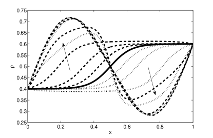
Figure 3: Two histories starting at the steady state profile (solid line), and leading to the same density profile with $a_{2}=0.3$, $a_{1}=0$, $a_{4}=0$ in Eq. 17 and $E=40$, $\rho_{0}=0.4$ with $\rho_{1}=0.6$. The two histories have the same statistical weight. One of the histories is depicted by dashed lines, and the other one by a dotted lines. Each line represents the density profile at a specific time, with the arrows showing the direction of the evolution in time.

Scanning of the full configuration space of the field $\rho_{f}(x)$ is impossible. Therefore, similar to [24], we constrain ourselves to finite-dimensional cuts. In particular, we first focus on smooth long wave length structures. To this end, we consider configurations of the form

$$\rho_{f}\left(x\right)=\bar{\rho}(x)+a_{1}\sin\left(\pi x\right)+a_{2}\sin\left(2\pi x\right)+a_{4}\sin\left(4\pi x\right)\ .$$ (17)

$a_{1}$, $a_{2}$ and $a_{4}$ loosely measure the size of the deviation from the most probable configuration $\bar{\rho}(x)$ at different wavelengths. Their values are constraint since the density is bound between $0\leq\rho(x)\leq 1$. We have verified that the exact choice of the functions (sine or other) describing the long wavelength behavior is not important for the overall structure of the results presented.

Our interest, as stated above, is identifying configurations at which the LDF is singular. As will become evident, to do so it is useful to employ the symmetries of the problem. We consider boundary conditions such that

$$\rho_{0}=0.5-\delta\quad;\quad\rho_{1}=0.5+\delta\ .$$ (18)

Note that under this choice of boundary conditions $\bar{\rho}(x)$ satisfies a particle-hole symmetry so that under the exchange $x\to-x$ and $\rho\to 1-\rho$ the most probable profile returns to itself. While a structure similar to what we find emerges for other choices of boundary conditions the results have a simpler form for this choice. In particular, for this choice $a_{2}$ and $a_{4}$ are deviations from $\bar{\rho}(x)$ which satisfy the particle-hole symmetry while $a_{1}$ breaks the symmetry.

Following the procedure outlined above we use the mapping, Eq. 15, to scan systematically, on the finite dimensional cuts, for cases where multiple saddle point solutions occur by looking for multiple $\varphi$ solutions of the differential equation for the same $\rho_{f}$. This is carried out numerically by using an extended ‘shooting’ algorithm [41] whose details are given in A. For the purpose of the discussion here we note that eventually the solutions are obtained by breaking the interval $\left[0,1\right]$ to $L$ bins. The accuracy of the solution increases with $L$.

We now describe the singular structures which we identify using this method.

4.1 The appearance and characterization of Ising-like (cusp) singularities

Consider first profiles such that $a_{1}=0$ and $a_{4}=0$ with $a_{2}$ non-zero. Such profiles are particle-hole symmetric. We find numerically that for large enough values of $E$ there is a critical value of $a_{2}$ for which multiple solutions of the saddle-point equations appear. An example is shown in Fig. 3 where the two locally minimizing histories are shown (an extra locally maximizing solution is also present but not shown). Note that, due to the symmetry, the two histories are connected through a particle-hole symmetry transformation, and both give the same value for the action in Eq. 10. In Fig. 4 we show the minimal value of $E$, denoted by $E_{c}$, for which two minimizing solutions appear for different values of $a_{2}$ for a specific choice of $\rho_{0}$ and $\rho_{1}$ (we have verified that the qualitative results are insensitive to this choice). Note that 1) there is a minimal value of $a_{2}$ above which degenerate, namely with equal values of the action, solutions appear and 2) there is a minimal value of the field $E$ below which a singularity never appears in the LDF (this value is considerably higher than the value of the field, $E\simeq 0.81$ for this choice of boundary conditions, at which the system is in equilibrium). Namely, singularities of the LDF appear only for conditions where the field $E$ is large enough, and for “large enough” deviations from the most probable configuration.

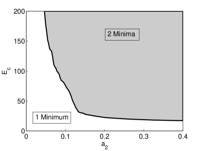
Figure 4: Minimum field $E_{c}$ required for an Ising-like (cusp) singularity, versus amplitude of the sine for the profile $\rho_{f}\left(x\right)=\bar{\rho}\left(x\right)+a_{2}\cdot\sin\left(2\pi x\right)$, where $\bar{\rho}\left(x\right)$ is the average profile for the PASEP with $\rho_{0}=0.4,\,\rho_{1}=0.6$. In the shaded area, two degenerate minimizing histories coexist. The border line is a second-order transition line.

The plane depicted in Fig. 4 contains a region in configuration space where two degenerate histories, which we denote by $h_{1}$ and $h_{2}$ (in the sense that they lead to the same value of the action from Eq. 10) coexist. If we make $a_{1}>0$ but small, the particle-hole symmetry is broken between the two histories and now one of the histories, say $h_{1}$, leads to a lower value of the action than the other. On the other hand for $a_{1}<0$, $h_{2}$ leads to a lower value of the action. Therefore, at $a_{1}=0$ there is a first-order-line singularity of the LDF. For a given value of $E$, as $a_{2}$ is decreased the two distinct histories merge into a single history, much like a critical point in usual phase transitions (or a cusp catastrophe). These results are illustrated in Fig. 5 where the resulting large deviation for a given value of $E$ in the $a_{1}$, $a_{2}$ plane is shown. Note that as $a_{1}$ is increased (for large enough $a_{2}$) the two solutions initially coexist (with one dominating the LDF) until eventually for large enough $a_{1}$ one of the solutions disappears. We comment that because of numerical precision seeing the singularity in the plotted lines of equal LDF value is rather hard. Their existence is most easily obtained by tracking where solutions appear and disappear.

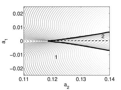
Figure 5: An Ising-like (cusp) singularity in the small E regime. Along the plotted lines the value of LDF is constant. The field strength is $E=40$ and the boundary conditions are $\rho_{l}=0.4\,;\,\rho_{r}=0.6$. The solid line is the border between the area with one minimum and the area with two minima. The dashed line is a first order transition line. On that line, two distinct histories, which have the same statistical weight, minimize the action. All the lines meet at an analogue of a critical point (cusp).

To describe the singularities we follow [25] and use a Landau like theory with a $Z_{2}$ symmetry. We look at the behavior of the LDF, $\phi\left[\rho\right]$, in the vicinity of the critical configuration $\rho_{f}^{cusp}$. As stated before, for a given $\rho_{f}$ on the switching line, there are two minimizing degenerate histories, $h_{1}\left(x,t\right)$ and $h_{2}\left(x,t\right)$. To build the Landau theory we introduce

$$a=\left[\int\left(\rho_{f}-\rho_{f}^{cusp}\right)^{2}\mathrm{d}x\right]^{\nicefrac{{1}}{{2}}}$$ (19)

as the distance of the configuration $\rho_{f}$ from $\rho_{f}^{cusp}$. Then we define a coordinate system $\left(a,b\right)$ with $\rho_{f}^{cusp}$ at the origin, $\hat{a}$ directed along the switching line and positive on the switching line, and $\hat{b}$ orthogonal to $\hat{a}$. In analogy with Landau mean-field theory, $a$ plays the role of the temperature ‘distance’ from the critical point and $b$ the role of the magnetic field. Let

$$\rho^{avg}\left(x,t\right) = \frac{1}{2}\left[h_{1}\left(x,t\right)+h_{2}\left(x,t\right)\right],$$

$$\delta\rho\left(x,t\right) = \frac{1}{2}\left[h_{1}\left(x,t\right)-h_{2}\left(x,t\right)\right],$$ (20)

$$u\left(x,t\right) = \delta\rho/\left\|\delta\rho\right\|$$

and

$$\Delta=\left\|\delta\rho\right\|$$ (21)

where $\left\|\delta\rho\right\|^{2}=\int\left[\delta\rho\left(x,t\right)\right]^{2}\mathrm{d}x\mathrm{d}t$ quantifies the distance between the two histories. Note that at the cusp, where the two histories coincide, $\Delta=0$. As will shortly become clear $\Delta$, which measures the distance between the two histories, is the order parameter of the Landau theory.

On the switching line $b=0$ and $\phi\left[\rho_{f},h_{1}\right]$ and $\phi\left[\rho_{f},h_{2}\right]$ are both minimizing histories with the same weight. Hence the function

$$s_{\rho_{f}}\left(q\right)=\phi\left[\rho_{f},\,\rho^{avg}+q\cdot u\right]$$ (22)

admits two minima, at $q=\pm\Delta$. In order to capture this behavior of two minima converging to one at a ‘critical’ point, we use the simplest analytical form possible:

$$\tilde{s}\left(q\right)=s\left(q\right)-s\left(0\right)=c_{4}q^{4}+ac_{2}q^{2}+bc_{1}q,$$ (23)

with $c_{1},c_{2},c_{4}>0$. $q$ is a selector between histories. Being so, it contains information which is inherently non-local both in time and space. At small $a$ and $b=0$, $\tilde{s}\left(q\right)$ has two minima, at $q_{min}\propto\pm\sqrt{a}$. Hence $\Delta\propto\sqrt{a}$ in direct analogy with a Landau theory, with an order parameter critical exponent $\beta$ with a value of $\nicefrac{{1}}{{2}}$.

In order to test the analogy, we generated a log-log plot of $\Delta\left(a\right)$, and measured the slope, $\beta$. In Fig. 6 we plot the value of the resulting measured exponent $\beta$ as a function of the number of bins, $L$, used in the numerics. The results strongly suggest that $\beta\rightarrow\nicefrac{{1}}{{2}}$ as $L\rightarrow\infty$.

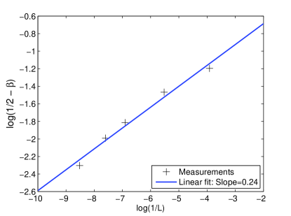
Figure 6: Critical exponent measurements for the cusp singularity in the WASEP model. The graph shows the approach of the critical exponent $\beta$, for different numerical precisions. $L$ is the number of bins taken inside the interval $\left[0,1\right]$. See main text for more details. One can witness that as the numerical precision rises the critical exponent approaches a value of 0.5.

4.2 Tricritical like singularities

It is natural to ask if there exist more complicated situations, where more than two solutions coexist. Indeed, as we now show, as the strength of the field is increased we find that a region with five extremal coexisting solutions (three locally minimizing and two locally maximizing) appears. In Fig. 7 we show for different values of $E$ the number of solutions in the $a_{2}$, $a_{4}$ plane for $a_{1}=0$. Namely, final configurations with a particle-hole symmetry. Note that due to the symmetry on this plane solutions related by particle-hole symmetry are degenerate.

For small $E$ we see that there is only one solution for each final configuration (data not shown). As $E$ increases a region with two locally minimizing solutions appears as described in the previous section. More interesting, for larger $E$ we find a region with three locally minimizing solutions (of a total of five solutions). For the smaller values of $E$ it is present only for large enough values of $a_{2}$ and $a_{4}$ (large enough deviations) while as $E$ increases the region covers a larger portion of the two dimensional cut. When three locally minimizing solutions are present we find that one obeys the particle-hole symmetry and the other two break it (data not shown). The structure is very close to that which emerges from a Landau theory of a tricritical point. The tricritical point occurs when the regions with one, two and three solutions meet.

Note that inside the three solutions area a line where the LDF is singular appears. This line is a transition due to a competition between the one minima with a particle-hole symmetric time evolution and the other two which are degenerate and break the particle hole symmetry. This behavior is, again, in direct analogy to a Landau theory of a tricritical point. The transition between the two is first-order. The transition line meets a second-order transition line as in a usual tricritical point structure. Note that along the lines where the region with three solutions turns into a two solution region the LDF is not singular but changes smoothly. Again, as in the discussion of the Ising-like singularity, inferring the singularities from the lines of equal LDF value can be misleading and it is best to track the number of solutions and their behavior. Therefore within the numerics we can only estimate the location of the singularities. Indeed, for intermediate values of the field even at regions where $3$ solutions were clearly visible it was numerically hard to identify the first order line.

In direct analogy to the previous section also here a Landau theory can be constructed. However, our numerics are not good enough to verify the expected exponents associated with the tricritical point.

In the next section we show that when $E\to\infty$ tricritical point type singularities (and much more complicated) appear. In that case the structure of the singularity is described exactly by a Landau-like theory.

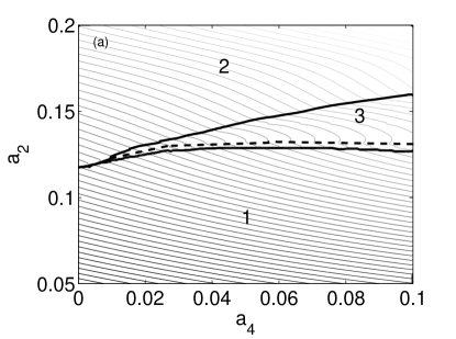
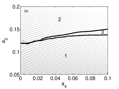
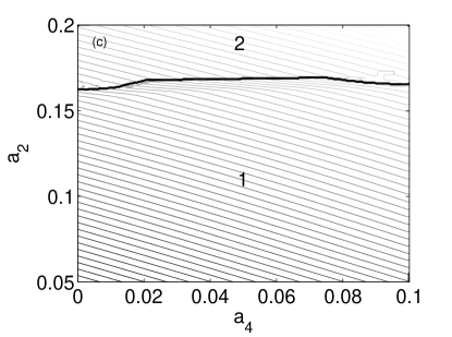
Figure 7: ‘Phase diagrams’ in the $a_{2},\,a_{4}$ plane for (a) $E=50$, (b) $E=40$ and (c) $E=25$ (from top to bottom). The numbers denote the number of locally minimizing solutions in the plane. Along the thin line the value of the LDF is constant. The thick solid lines are borders between areas with different numbers of locally minimizing histories (they are not necessarily transition lines). The tip of the three minima area is where the tricritical-like point resides. In (a) the dashed line (a guide to the eye) is a first order transition line where all three minima give the same value for the action, and the LDF shows a singularity structure manifested in a clear “break” of the equipotential lines. Below this line, the single minimum has the lowest value, and above this line the two degenerate minima have a lower value and they determine the value of the LDF. The border between the one minimum and two minima area is a second order transition line. In (b) the first order transition line almost overlaps the line separating the one and the three minima areas, so we do not show it. Note how the three minima area is not seen for (c) $E=25$ and only a cusp singularity remains (the transition is on the boundary between one and two minima).

5 The LDF at infinite bulk drive

Next, we turn to consider the limit $E\to\infty$. In the common terminology this corresponds to a PASEP and as before $E$ is in the positive direction with $\rho_{1}>\rho_{0}$. Similar to the above discussion we consider specific cuts of the configuration space $\rho(x)$. The main points of the discussion which follows are: 1) Within the subspaces studied we can identify configurations at which the LDF is singular. 2) Around appropriate configurations the singular behavior of the LDF can be described exactly by a Landau like theory. The simplest ones will be, as above, cusp (or Ising) singularities and an analogue of a tricritical point. More striking is the identification of configurations at which an arbitrary number of histories reach the same final configuration with the same weight. This leads to an analogue of an arbitrary order multicritical point. We note that while an exact correspondence between the order parameter defined in the previous section and the one used in this section is not shown their general behavior is identical.

To show the above results we use the $E\to\infty$ limit expression for the LDF obtained in [12, 14]. There it was shown that

$$\phi\left[\rho_{f}\left(x\right)\right]=-\mathcal{K}\left(\rho_{0},\rho_{1}\right)+\mathcal{F}\left[\rho_{f}\left(x\right)\right]+\inf_{0<y<1}\mathcal{G}\left[\rho_{f}\left(x\right),y\right]\ ,$$ (24)

where

$$\mathcal{K}\left(\rho_{0},\rho_{1}\right) = \min\left[\log\rho_{0}\left(1-\rho_{0}\right),\log\rho_{1}\left(1-\rho_{1}\right)\right]\ ,$$ (25)

$$\mathcal{F}\left[\rho_{f}\left(x\right)\right] = \int_{0}^{1}\mathrm{d}x\left[\rho_{f}\left(x\right)\log\left(\rho_{f}\left(x\right)\right)+\left(1-\rho_{f}\left(x\right)\right)\log\left(1-\rho_{f}\left(x\right)\right)\right]\ ,$$

and $\mathcal{G}$ is given by

$$\mathcal{G}\left[\rho_{f}\left(x\right),y\right] = \int_{0}^{y}\mathrm{d}x\left[\rho_{f}\left(x\right)\log\left(1-\rho_{0}\right)+\left(1-\rho_{f}\left(x\right)\right)\log\left(\rho_{0}\right)\right]$$

$$+ \int_{y}^{1}\mathrm{d}x\left[\rho_{f}\left(x\right)\log\left(1-\rho_{1}\right)+\left(1-\rho_{f}\left(x\right)\right)\log\left(\rho_{1}\right)\right]\ .$$

The result can be obtained by taking the $E\to\infty$ limit using the results of Sec. 3.

Clearly, any singular behavior of the functional can appear only in $\mathcal{G}$. To this end, it is convenient to only consider the behavior of

$$g\left[\rho_{f}\left(x\right)\right]=\inf_{y}\mathcal{G}\left[\rho_{f}\left(x\right),y\right]\,.$$ (27)

The discussion of Sec. 3 can be shown to imply that for a given final configuration $\rho_{f}(x)$ each locally minimizing value of $y$ corresponds to a particular choice of history which leads to it [14].

Next, for simplicity we consider density profiles of the form

$$\rho_{f}\left(x\right)=\left(\frac{1}{2}-\delta\right)+2\delta\cdot x+\sum_{n=1}^{2n_{max}}a_{n}\sin\left(n\pi x\right)\ ,$$ (28)

where $\delta\in\left(0,\nicefrac{{1}}{{2}}\right]$ and use the boundary conditions of Eq. 18. It is straightforward to show that profiles which cross $\rho=\nicefrac{{1}}{{2}}$ $k$ times have $k$ extremal histories leading to them [14]. Note, that $\rho_{f}$ has an implicit dependence on $n_{max}$ which we suppress most of the time for brevity. These profiles will allow us to look at different subspaces of $\phi\left[\rho_{f}\left(x\right)\right]$ by characterizing the function $\rho_{f}\left(x\right)$ using the vector $\left(a_{1},...,a_{2n_{max}}\right)$. While singularities are likely to occur for other configurations and boundary conditions, this particular choice allows for a particle-hole symmetry to be exploited and analytical results to be obtained. This gives a simple mapping of the problem to a Landau theory around specific values of $\left(a_{1},...,a_{2n_{max}}\right)$.

5.1 Mapping to Landau theory of different types

We start by considering profiles where cusp and tricritical-like singularities appear. As before, for cusp singularities there is a region in configuration space where two locally minimizing histories lead to the same final configuration. The Landau like expansion is carried around the point where the two histories merge into one. For the tricritical point there is a region where three locally minimizing solutions lead to the same final configuration and the expansion is carried around the point where the three histories merge into one. Finally, the generalization to higher order cases will be derived.

To carry out the mapping we define $m=y-1/2$ and expand $\mathcal{G}(m)$ in powers of $m$. A straightforward calculation shows that

$$\mathcal{G}\left(m\right)=2\log\left(\frac{1+\delta}{1-\delta}\right)\cdot\sum_{n=0}^{\infty}c_{n}m^{n}\,.$$ (29)

Here $c_{0}$ is a constant (which can be ignored) and we have extracted the constant $2\log\left(\frac{1+\delta}{1-\delta}\right)$ to simplify the expressions for the coefficients $c_{n}$. Using Eq. 28, it can be shown that

$$c_{1}= \frac{1}{2}\left(2\left.\rho\right|_{m=0}-1\right)=\sum_{n\in odd}\left(-1\right)^{\frac{n-1}{2}}a_{n},$$ (30a)

$$c_{2}= \frac{1}{2}\left.\frac{\mathrm{d}}{\mathrm{d}m}\rho\right|_{m=0}=\frac{1}{2}\left[2\delta+\sum_{n\in even}\left(-1\right)^{\frac{n}{2}}n\pi a_{n}\right],$$ (30b)

and more generally (for $k>1$)

$$c_{2k-1}= \frac{1}{\left(2k-1\right)!}\left.\frac{\mathrm{d}^{2k-2}}{\mathrm{d}m^{2k-2}}\rho\right|_{m=0}=\frac{\left(-1\right)^{k-1}}{\left(2k-1\right)!}\sum_{n\in odd}\left(-1\right)^{\frac{n-1}{2}}\left(n\pi\right)^{2k-2}a_{n}\,.$$ (30aea)

$$c_{2k}= \frac{1}{\left(2k\right)!}\left.\frac{\mathrm{d}^{2k-1}}{\mathrm{d}m^{2k-1}}\rho\right|_{m=0}=\frac{\left(-1\right)^{k+1}}{\left(2k\right)!}\sum_{n\in even}\left(-1\right)^{\frac{n}{2}}\left(n\pi\right)^{2k-1}a_{n}\,,$$ (30aeb)

Notice that $c_{n}$ with $n$ odd include only $a_{n}$ coefficients with $n$ odd and similarly $c_{n}$ with $n$ even include only $a_{n}$ with $n$ even. This is a direct consequence of the choice of boundary conditions and profiles. Profiles which involve only $a_{n}$ with even values of $n$ have a particle-hole symmetry while those with $a_{n}$ with $n$ odd break this symmetry.

Finally, note that $g\left[\rho_{f}\left(x\right)\right]=\inf_{m}\mathcal{G}\left[\rho_{f}\left(x\right),\,m\right]$ in analogy with a Landau free energy with $m$ playing the role of the order parameter. We now turn to discuss specific configurations where a singular LDF appears.

5.1.1 Ising-like or Cusp singularities:

Here we consider profiles of the form:

$$\rho_{f}\left(x\right)=\left(\frac{1}{2}-\delta\right)+2\delta\cdot x+a_{1}\sin\left(\pi x\right)+a_{2}\sin\left(2\pi x\right)\ .$$ (30aeaf)

Substituting this particular choice into Eqs. 30ae we obtain

$$c_{1}= a_{1}\,,$$ (30aeaga)

$$c_{2}= \delta-\pi a_{2}\,,$$ (30aeagb)

$$c_{3}= -\frac{\pi^{2}}{6}a_{1}\,,$$ (30aeagc)

$$c_{4}= \frac{\pi^{3}}{3}a_{2}\,.$$ (30aeagd)

While in general $c_{n}$ with $n>4$ appear it is clear that by choosing $c_{2}$ and $c_{1}$ small they can be neglected. Using the standard arguments of the Landau theory the singular behavior of the LDF can be captured by

$$\mathcal{G}\left(m\right)\simeq 2\log\left(\frac{1+\delta}{1-\delta}\right)\cdot\left(c_{0}+a_{1}m+(\delta-\pi a_{2})m^{2}+\frac{\pi^{3}}{3}a_{2}m^{4}\right)\;,$$ (30aeagah)

where the expansion is taken about the critical-point

$$\left(a_{1}^{\star},\,a_{2}^{\star}\right)=\left(0,\,\frac{\delta}{\pi}\right)\ .$$ (30aeagai)

Note that the coefficient of $m^{4}$ is positive near the critical point. Following a standard Landau theory it is clear that the structure of $\mathcal{G}\left(m\right)$ implies that there is a first-order like transition line (on which the derivative of the LDF has a discontinuity) ending in a critical-point analogue. Furthermore, as before this implies that approaching the critical point along this line the minimizing value of $m$, denoted by $m^{\star}$ gives $m^{\star}\propto(\delta-\pi a_{2})^{\nicefrac{{1}}{{2}}}$ with other standard Landau theory results following.

Fig. 8 demonstrates the results of a numerical calculation of the number of minima for $\mathcal{G}\left(a_{1},\,a_{2},\,m\right)$ around the critical point, and of the value of $m^{\star}$. At each point $\left(a_{1},\,a_{2}\right)$ in the configuration space the order parameter is the value of $m$ which minimizes $\mathcal{G}\left(a_{1},\,a_{2},\,m\right)$. This value is obtained by minimizing $\mathcal{G}$ numerically. The region in configuration space where two locally minimizing solutions exist is also shown.

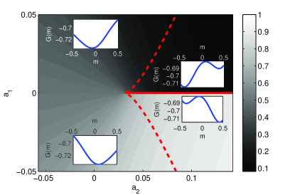
Figure 8: The ‘phase diagram’ for profiles of the form $\rho_{f}\left(x\right)=\frac{1}{2}-\delta+2\delta\cdot x+a_{1}\sin\left(\pi x\right)+a_{2}\sin\left(2\pi x\right)$ with $\delta=0.1$, which demonstrates an Ising singularity (or cusp catastrophe). The background color represents the value of the order parameter (black is for lower values, white for higher values). The insets show the function $\mathcal{G}(m)$ in different areas of the phase space. The dashed line represents the border between a one minimum area in $\mathcal{G}$, and a two minima area. The solid line represents a first order transition. The point where all the lines meet is the analogue of a critical point.

5.1.2 Tricritical point analogue (butterfly catastrophe):

We now move to look at profiles in the subspace of configurations defined by

$$\rho_{f}\left(x\right)=\frac{1}{2}-\delta+2\delta\cdot x+a_{1}\sin\left(\pi x\right)+a_{2}\sin\left(2\pi x\right)+a_{4}\sin\left(4\pi x\right).$$ (30aeagaj)

In a manner similar to the one we used to find the cusp critical point, we look at the first six coefficients of Eq. 29 to find

$$c_{1}= a_{1}\,,$$ (30aeagaka)

$$c_{2}= \left(\delta-\pi a_{2}+2\pi a_{4}\right)\,,$$ (30aeagakb)

$$c_{3}= -\frac{\pi^{2}}{6}a_{1}\,,$$ (30aeagakc)

$$c_{4}= \frac{\pi^{3}}{3}\left(a_{2}-8a_{4}\right)\,,$$ (30aeagakd)

$$c_{5}= \frac{\pi^{4}}{120}a_{1}\,,$$ (30aeagake)

$$c_{6}= \frac{2\pi^{5}}{45}\left(-a_{2}+32a_{4}\right)\,.$$ (30aeagakf)

Higher order terms do not vanish. Using standard arguments a proper choice of $c_{1},c_{2},c_{3},c_{4},c_{5},c_{6}$ which gives $m^{\star}$ small, justifies the truncation of the series. It is rather straightforward to check that these values correspond to a realizable configuration where $0\leq\rho_{f}(x)\leq 1$. Similar to an expansion about a tricritical point (or a butterfly catastrophe) we find

$$\mathcal{G}\left(m\right) \simeq 2\log\left(\frac{1+\delta}{1-\delta}\right)\cdot\left(c_{0}+a_{1}m+\left(\delta-\pi a_{2}+2\pi a_{4}\right)m^{2}-\frac{\pi^{2}}{6}a_{1}m^{3}\right.$$

$$\left.+\frac{\pi^{3}}{3}\left(a_{2}-8a_{4}\right)m^{4}+\frac{2\pi^{5}}{45}\left(-a_{2}+32a_{4}\right)m^{6}\right)\;,$$

where the tricritical point is specified by

$$\left(a_{1}^{\star},a_{2}^{\star},a_{4}^{\star}\right)=\left(0,\frac{4}{3}\frac{\delta}{\pi},\frac{\delta}{6\pi}\right)\,.$$ (30aeagakam)

Note that the coefficient of $m^{6}$ around the tricritical point is positive. On the $a_{1}=0$ plane there is an analogue of a $\lambda$-line [42], with a second order phase transition line connected to a first-order transition line at the tricritical point. As we approach that point along the $a_{2}=8a_{4}$ line the order parameter behaves as $m^{\star}\propto\left(\delta-\pi a_{2}+2\pi a_{4}\right)^{\nicefrac{{1}}{{4}}}$.

Fig. 9 demonstrates the above structure on the plane $a_{1}=0$. It is essentially a textbook tricritical behavior in configuration space. The figure also shows the corresponding $\mathcal{G}(m)$ at different locations in the plane.

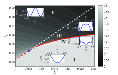
Figure 9: The ‘phase diagram’ for $\rho_{f}\left(x\right)=\rho_{0}+2\delta\cdot x+a_{2}\sin\left(2\pi x\right)+a_{4}\sin\left(4\pi x\right)$ with $\delta=0.1$. The background color represents the order parameter (black is for lower values, gray is for higher values), where a lower value was chosen where there were two competing values (due to the symmetry). The phase space is divided into 4 regions. In region (I) there is one minimum (corresponding to a symmetric history), in region (II) there are two symmetric minima, and in regions (III) and (IV) there are three different minima. The solid red line is a first order transition line where three different minimizing solutions coexist. The red-white line is a second order transition. The upper dashed white line is a crossing between having one/three minima, and the lower dashed white line is a crossing where one minimum transforms to a maximum and two extra minima. The blue dot where all the lines meet is a tricritical point . The insets show the function $\mathcal{G}(m)$ in different areas of the phase space.

5.1.3 Multicritical points:

With the above examples of singular behavior it is natural to ask if configurations where more than three locally minimizing solutions, which all give the same value of the LDF, exist. In analogy with the above results this should imply the existence of analogues of multicritical points of general order $s$. To identify such multicritical points we look for configurations where the first $2s-1$ derivatives of $\mathcal{G}(m)$ with respect to $m$ vanish. Close to such points (where $2s-1$ coefficients disappear), it is safe to say that the minimizing $m^{\star}$ is small, and so if the $2s$-th coefficient is positive it will be dominant. Then terms in the Landau expansion with $n>s$ can be neglected. In B we show that such a solution can be found, and that we need $n_{max}=s-1$ sine function in Eq. 28 to achieve that. The multicritical point $\left(a_{1}^{\star},a_{2}^{\star},...,a_{2n_{max}}^{\star}\right)$ is found at

$$a_{2n-1}^{\star}=0\,$$ (30aeagakan)

for the odd coefficients, while for the even coefficients we get

$$a_{2n}^{\star}=\frac{2\left(\left(s-1\right)!\right)^{2}}{n\pi\left(s-1+n\right)!\left(s-1-n\right)!}\delta\,.$$ (30aeagakao)

with $n$ between $1$ and $s-1$. For $c_{2s}$ we find

$$c_{2s}=\frac{\left(-1\right)^{s+1}}{\left(2s\right)!}\sum_{n=1}^{s-1}\left(-1\right)^{n}\left(2n\pi\right)^{2s-1}a_{2n}^{\star}=\frac{\left(-1\right)^{s+1}}{\left(2s\right)!}\sum_{n=1}^{s-1}\left(-1\right)^{n}\frac{4\left(2n\pi\right)^{2s-2}\left(\left(s-1\right)!\right)^{2}}{\left(s-1+n\right)!\left(s-1-n\right)!}\delta\,.$$ (30aeagakap)

By substituting numerically for $s$ it can be seen that this expression is positive for all $s$. This justifies the termination of the Landau expansion at $c_{2s}$. One can easily check the validity of the expressions by substituting $s=2$ for an Ising (cusp) singularity, and $s=3$ for a tricritical (butterfly) singularity, both of which were presented above.

Finally, to check that the coefficients $a_{n}$ correspond to realizable configurations with $0\leq\rho(x)\leq 1$ we plot the configurations for different orders of $s$ in Fig. 10. As can be seen all configurations are indeed realizable. In particular, it is easy to see (using standard Fourier methods) that for $s\rightarrow\infty$, the profile converges to:

$$\rho_{f,\,s\rightarrow\infty}^{\star}\left(x\right)\longrightarrow\frac{\rho_{1}+\rho_{0}}{2}.$$ (30aeagakaq)

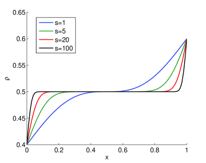
Figure 10: Plots of $\rho_{f}^{\star}\left(x\right)$ for different values of $s$. As $s$ increases, $\rho_{f}^{\star}$ is getting flatter. Each profile crosses the line $\rho=\nicefrac{{1}}{{2}}$ exactly once. A small deviation from these profiles will promptly generate multiple extremal histories leading to these profiles.

6 Summary and discussion

In this paper we focused on the structure of singularities in bulk driven transport models. With a finite bulk field (a WASEP) we demonstrated numerically that as the strength of the bulk bias increases analogues of critical and tricritical point singularities appear in configuration space. With the bulk drive infinite (a PASEP), we obtained an analytical mapping between the large deviation functional and an effective Landau theory. Remarkably, analogues of multicritical points of any order have been identified. The direct mapping to a Landau theory is not obvious. As discussed in [25] the applicability of the Landau theory relies on the fact that the Hessian matrix, which characterizes the stability of each history, has a single eigenvalue which vanishes at the (multi)critical point. While here the measurement of the Hessian proved too hard the exact mapping to a Landau theory in the infinite field case as well as the numerics of the exponent for a cusp singularity at small fields suggest that this is indeed the case. It is an interesting questions to see if other models can shown more complicated behaviors.

Finally, in the work presented above the Landau theory was proved only in the infinite field limit and without directly relating the order parameter to the histories. It would be interesting to see if this can be done rigorously.

Acknowledgments: We would like to thank Daniel Podolsky for many useful comments and discussions. The work has been supported by ISF and BSF grants.

Appendix A Shooting method for more than one solution

As discussed in the text, we are interested in detecting multiple solutions of the ordinary differential equation of the mapping Eq. 15. To do this we first rewrite the equation as a standard second order non-linear boundary value problem:

$$\varphi_{xx} =f\left(x,\varphi,\varphi_{x}\right)=\varphi_{x}\left(E-\varphi_{x}\right)\left(\frac{1}{1+e^{\varphi}}-\rho\right)\ ,$$

$$\varphi\left(0\right)=\varphi_{0}=\log\left(\frac{\rho_{0}}{1-\rho_{0}}\right)\quad,\quad\varphi\left(1\right)=\varphi_{1}=\log\left(\frac{\rho_{1}}{1-\rho_{1}}\right)\ .$$ (30aeagakar)

Common algorithms for solving such problems, such as the shooting or relaxation methods, usually look for one solution [41]. In the case of multiple solutions, the solution obtained by these methods is dependent on the initial guess.

To this end, in order to find all the possible solutions of the equation, we used a modified approach, in which we use a range of possible values for $\varphi_{x}\left(0\right)$. For each such value we integrate the differential equation using standard initial value problem methods, and look at the value $\varphi_{1}^{{}^{\prime}}\left(\varphi_{x}\left(0\right)\right)$, the value of $\varphi$ obtained at the right of the interval given the initial value of $\varphi_{x}\left(0\right)$. We then look at the function:

$$g\left(\varphi_{x}\left(0\right)\right)=\varphi_{1}^{{}^{\prime}}\left(\varphi_{x}\left(0\right)\right)-\varphi_{1}\ .$$ (30aeagakas)

Whenever $g\left(\varphi_{x}\left(0\right)\right)=0$, the solution obtained by the integration of the differential equation for that initial condition is a solution to the original boundary value problem. The problem is now reduced to finding the roots of $g\left(x\right)$. We do that by first calculating $g\left(x\right)$ on a coarse range of values, find the intervals where we detect a crossing with zero. Then we feed these intervals as initial intervals to a root finding algorithm, such as Newton-Raphson. Since the function $g\left(x\right)$ is very noisy (see Fig. 11), it may generate too many crossings with zero, which might produce an excessive number of solutions.

To avoid over-counting the number of solutions, we put the solutions obtained as an initial guess for a high accuracy boundary value problem solver, on $L$ bins in the interval $\left[0,1\right]$. Obviously the numerical accuracy of the results depends on the value of $L$. Near a critical point, all the solutions are very close to each other, so the ability to distinguish between the solutions is most vital near the critical points (see main text). Typical values of $L$ used were between $100$ and $5000$.

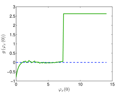
Figure 11: An example of the function $g\left(\varphi_{x}\left(0\right)\right)$, defined in Eq. 30aeagakas. Note how the function is very noisy and could potentially yield excessive results if we do not double-check to see that it really implies the existence of different solutions. We used the fact that $\varphi$ is monotonic to stop integration if the value $\varphi\left(c\right)$ at some point $c\in\left(0,1\right)$ exceeds the value of $\varphi_{1}$ by far. This is why the function is clipped at the end.

Appendix B Derivation of coefficients for the critical density profile at infinite bulk drive

Here we derive the coefficients of the multicritical profile of order $s$, namely Eqs. 30aeagakan, 30aeagakao. We start from Eqs. 30aea, 30aeb for the coefficients. Our goal is to solve for the first $2s-1$ coefficients. It is evident that $c_{n}$ with even and odd $n$ involve only even and odd sine functions, respectively. We can use this fact and obtain two sets of uncoupled equations for the coefficients of the multicritical profile of order $s$. We denote this point by $\left(a_{1}^{*},a_{2}^{*},...,a_{s}^{*}\right)$. For the odd coefficients we have the following set of equations

$$A\cdot\boldsymbol{a}_{odd}^{*}=\left(\begin{array}[]{cccc}1&-1&\dots&\left(-1\right)^{n+1}\\ -\pi^{2}&\left(3\pi\right)^{2}&\dots&\left(-1\right)^{n}\left(\left(2n-1\right)\pi\right)^{2}\\ \vdots&&\ddots&\vdots\\ \left(-1\right)^{k}\left(\pi\right)^{2k-2}&\left(-1\right)^{k+1}\left(3\pi\right)^{2k-2}&\cdots&\left(-1\right)^{k+n}\left(\left(2n-1\right)\pi\right)^{2k}\end{array}\right)\left(\begin{array}[]{c}a_{1}^{*}\\ a_{3}^{*}\\ \vdots\\ a_{2s-1}^{*}\end{array}\right)=\left(\begin{array}[]{c}0\\ 0\\ \vdots\\ 0\end{array}\right)\,,$$ (30aeagakata)

and for the even coefficients we have

$$B\cdot\boldsymbol{a}_{even}^{*}=\left(\begin{array}[]{cccc}-2\pi&4\pi&\dots&\left(-1\right)^{n}2n\pi\\ \left(2\pi\right)^{3}&-\left(4\pi\right)^{3}&\dots&\left(-1\right)^{n+1}\left(2n\pi\right)^{3}\\ \vdots&&\ddots&\vdots\\ \left(-1\right)^{k}\left(2\pi\right)^{2k-1}&\left(-1\right)^{k+1}\left(4\pi\right)^{2k-1}&\cdots&\left(-1\right)^{k+n}\left(2n\pi\right)^{2k-1}\end{array}\right)\left(\begin{array}[]{c}a_{2}^{*}\\ a_{4}^{*}\\ \vdots\\ a_{2s-2}^{*}\end{array}\right)=\left(\begin{array}[]{c}2\delta\\ 0\\ \vdots\\ 0\end{array}\right)\,.$$ (30aeagakatb)

In both matrices we used the indices $k$ and $n$ to enumerate the rows and columns, respectively. The matrices $A,\,B$ are both regular. To see that, we note that the determinant of the matrix $A$ is equal up to a sign to that of the Vandermonde matrix [43]

$$\tilde{A}=\left(\begin{array}[]{cccc}1&1&\dots&1\\ \pi^{2}&\left(3\pi\right)^{2}&\dots&\left(\left(2n-1\right)\pi\right)^{2}\\ \vdots&&\ddots&\vdots\\ \left(\pi^{2}\right)^{k-1}&\left(\left(3\pi\right)^{2}\right)^{k-1}&\cdots&\left(\left(\left(2n-1\right)\pi\right)^{2}\right)^{k-1}\end{array}\right)\,,$$ (30aeagakatau)

which is regular. The determinant of the matrix $B$ is equal to that of another matrix

$$\tilde{B}=\left(\begin{array}[]{cccc}-2\pi&4\pi&\dots&\left(-1\right)^{n}2n\pi\\ -\left(2\pi\right)^{3}&\left(4\pi\right)^{3}&\dots&\left(-1\right)^{n}\left(2n\pi\right)^{3}\\ \vdots&&\ddots&\vdots\\ -\left(2\pi\right)^{2k-1}&\left(4\pi\right)^{2k-1}&\cdots&\left(-1\right)^{n}\left(2n\pi\right)^{2k-1}\end{array}\right)\,,$$ (30aeagakatav)

which can be decomposed into two matrices, both of which are regular

$$\tilde{B}=\left(\begin{array}[]{cccc}1&1&\dots&1\\ \left(2\pi\right)^{2}&\left(4\pi\right)^{2}&\dots&\left(2n\pi\right)^{2}\\ \vdots&&\ddots&\vdots\\ \left(\left(2\pi\right)^{2}\right)^{k}&\left(\left(4\pi\right)^{2}\right)^{k}&\cdots&\left(\left(2n\pi\right)^{2}\right)^{k}\end{array}\right)\cdot\left(\begin{array}[]{cccc}-2\pi&0&\dots&0\\ 0&4\pi&\dots&0\\ \vdots&&\ddots&\vdots\\ 0&0&\cdots&\left(-1\right)^{n}2n\pi\end{array}\right)\,.$$ (30aeagakataw)

Since the matrix $\tilde{B}$ is composed of two regular matrices, it is also regular, and so is the matrix $B$. It follows that the set of Eqs. 30aeagakat has a single solution. For the odd part it is clear that the only solution is the trivial solution, hence Eq. 30aeagakan. For the even part, Cramer’s rule [44] can be used to obtain a solution to the linear set of equations, which yields Eq. 30aeagakao.

References

References

- [1] Derrida B 2007 J. Stat. Mech. 2007 P07023
- [2] Bertini L, De Sole A, Gabrielli D, Jona-Lasinio G and Landim C 2005 Phys. Rev. Lett. 94 030601
- [3] Bodineau T and Derrida B 2005 Phys. Rev. E 72 066110
- [4] Lecomte V, Imparato A and Van Wijland F 2010 Prog. Theor. Phys. Supplement 184 276–289
- [5] Merhav N and Kafri Y 2010 J. Stat. Mech. 2010 P02011
- [6] Krapivsky P and Meerson B 2012 Phys. Rev. E 86 031106
- [7] Gorissen M, Lazarescu A, Mallick K and Vanderzande C 2012 Phys. Rev. Lett. 109 170601
- [8] Meerson B and Sasorov P V 2013 J. Stat. Mech. 2013 P12011
- [9] Akkermans E, Bodineau T, Derrida B and Shpielberg O 2013 Europhys. Lett. 103 20001
- [10] Derrida B, Evans M, Hakim V and Pasquier V 1993 J. Phys. A: Math. Gen. 26 1493
- [11] Derrida B, Lebowitz J and Speer E 2002 J. Stat. Phys. 107 599–634
- [12] Derrida B, Lebowitz J and Speer E 2003 J. Stat. Phys. 110 775–810
- [13] Enaud C and Derrida B 2004 J. Stat. Phys. 114 537–562
- [14] Bertini L, De Sole A, Gabrielli D, Jona-Lasinio G and Landim C 2010 J. Stat. Mech. 2010 L11001
- [15] Bunin G, Kafri Y and Podolsky D 2012 Europhys. Lett. 99 20002
- [16] Cohen O and Mukamel D 2011 J. Phys. A: Math. Theo. 44 415004
- [17] Cohen O and Mukamel D 2014 Phys. Rev. E 90(1) 012107 URL http://link.aps.org/doi/10.1103/PhysRevE.90.012107
- [18] Kipnis C, Olla S and Varadhan S 1989 Communications on Pure and Applied Mathematics 42 115–137
- [19] Touchette H and Harris R J 2013 Large deviation approach to non-equilibrium systems Non-equilibrium Statistical Physics of Small Systems: Fluctuation Relations and Beyond ed Schuster H G, Klages R, Just W and Jarzynski C (John Wiley & Sons)
- [20] Spohn H 1983 J. Phys. A: Math. Gen. 16 4275
- [21] Dorfman J, Kirkpatrick T and Sengers J 1994 Annu. Rev. Phys. Chem. 45 213–239
- [22] De Zarate J M O and Sengers J V 2006 Hydrodynamic fluctuations in fluids and fluid mixtures (Elsevier)
- [23] Bunin G, Kafri Y, Lecomte V, Podolsky D and Polkovnikov A 2013 J. Stat. Mech. 2013 P08015
- [24] Bunin G, Kafri Y and Podolsky D 2012 J. Stat. Mech. 2012 L10001
- [25] Bunin G, Kafri Y and Podolsky D 2013 J. Stat. Phys. 1–24
- [26] Graham R and Tél T 1984 Phys. Rev. Lett. 52 9–12
- [27] Graham R and Tél T 1984 J. Stat. Phys. 35 729–748
- [28] Graham R and Tél T 1985 Phys. Rev. A 31 1109
- [29] Graham R and Tél T 1986 Phys. Rev. A 33 1322
- [30] Jauslin H 1987 Physica A: Statistical Mechanics and its Applications 144 179–191
- [31] Gilmore R 1992 Encyclopedia of Applied Physics
- [32] Blythe R and Evans M 2007 J. Phys. A: Math. Theo. 40 R333
- [33] Spohn H 1991 Large scale dynamics of interacting particles vol 174 (Springer-Verlag New York)
- [34] Sasamoto T 1999 J. Phys. A: Math. Gen. 32 7109
- [35] Blythe R, Evans M, Colaiori F and Essler F 2000 J. Phys. A: Math. Gen. 33 2313
- [36] Bertini L, De Sole A, Gabrielli D, Jona-Lasinio G and Landim C 2001 Phys. Rev. Lett. 87 040601
- [37] Bertini L, De Sole A, Gabrielli D, Jona-Lasinio G and Landim C 2002 J. Stat. Phys. 107 635–675
- [38] Martin P C, Siggia E D and Rose H A 1973 Phys. Rev. A 8(1) 423–437 URL http://link.aps.org/doi/10.1103/PhysRevA.8.423
- [39] Tailleur J, Kurchan J and Lecomte V 2008 J. Phys. A: Math. Theo. 41 505001
- [40] Bernfeld S R and Lakshmikantham V 1974 An introduction to nonlinear boundary value problems vol 6 (Academic Press New York)
- [41] Press W H 2007 Numerical recipes 3rd edition: The art of scientific computing (Cambridge university press)
- [42] Chaikin P M, Lubensky T C and Witten T A 2000 Principles of condensed matter physics vol 1 (Cambridge Univ Press)
- [43] Meyer C D 2000 Matrix analysis and applied linear algebra vol 2 (Siam)
- [44] Cramer G 1750 Introduction à l’analyse des lignes courbes algébriques (chez les frères Cramer et C. Philibert)