On the Causal Set-Continuum Correspondence

Abstract

We present two results which concern certain aspects of the question: when is a causal set well approximated by a Lorentzian manifold? The first result is a theorem which shows that the number-volume correspondence, if required to hold even for arbitrarily small regions, is best realized via Poisson sprinkling. The second result concerns a family of lattices in $1+1$ dimensional Minkowski space, known as Lorentzian lattices, which we show provide a much better number-volume correspondence than Poisson sprinkling for large volumes. We argue, however, that this feature should not persist in higher dimensions. We conclude by conjecturing a form of the aforementioned theorem that holds under weaker assumptions, namely that Poisson sprinkling provides the best number-volume correspondence in $3+1$ dimensions for spacetime regions with macroscopically large volumes.

1 Background

From the viewpoint of causal set theory, the continuum spacetime of general relativity is only fundamental to the extent that it provides a good approximation to an underlying causal set Sorkin_1 ; Sorkin_2 ; Sorkin_3 ; Dowker_1 ; Henson . Once a full dynamical theory of causal sets is available, it is necessary to judge whether or not the result of evolution looks anything like the universe we observe at low energies. Therefore, criteria must be established to determine how well a Lorentzian geometry $(M,g)$ approximates a causal set $(C,\prec)$. One natural criterion is to require the existence of an injective map $f:C\to M$ which preserves causal relations: $\forall$ $x,y\in C$, $x\prec y$ if and only if $f(x)\in J^{-}(y)$, where $J^{-}(y)$ is the set of all points in $M$ which lie in the causal past of $y$. We would then say that $C$ is embeddable in $M$. Of course, it is not very likely for a causal set which has emerged out of the dynamics to be exactly embeddable in any spacetime. Close to the discreteness scale, for instance, one would expect the causal set to be fairly chaotic. Therefore, a certain degree of coarse graining must be done before embedding is possible. It might also be necessary to introduce some notion of approximate embedding, because matching all causal relations exactly (and there would be a lot of them) seems too stringent a requirement. Once these issues are settled and embedding is possible, one last piece of information is required: scale. This is because preserving causal relations cannot distinguish between spacetimes whose metrics are conformally related. Causal sets contain information about scale implicitly through counting of elements, because they are locally finite (i.e. discrete). To make use of this property, one also requires a number-volume (N-V) correspondence: the number $N_{S}$ of embedded points in any spacetime region $S\subset M$ should “reflect” its volume $V_{S}$:

$$N_{S}\approx\rho V_{S}=\rho\int_{S}\sqrt{-g(x)}d^{D}x,$$ (1)

where $\rho$ is a constant, thought to be set by the Planck scale, which represents the number density of points. Of course, this correspondence cannot be exactly true, the most obvious reason being that $\rho V_{S}$ is not always an integer. Also, for any embedding, there would always be infinitely many empty regions meandering through the embedded points. These issues can be addressed by first settling on the types of “test regions” $S$, and then requiring the correspondence in a statistical sense. To do so, let us first note that the causal set-continuum correspondence is only physically meaningful on scales much larger than the discreteness scale. Therefore, $S$ should be a region whose spacetime volume is much larger than that set by the discreteness scale. The shape of $S$ can be picked to disallow regions that meander through the embedded points but have large volumes. A natural choice, given that spacetime is Lorentzian, is the causal interval $I(x,y)$: given any two timelike points $x\prec y\in M$, $I(x,y)$ is the collection of all points in the causal future of $x$ and the causal past of $y$. Having decided on the types of test regions, the number-volume correspondence can be formulated as follows: pick at random $M$ causal intervals $S_{1},S_{2},\dots,S_{M}$ with the same volume $V\gg\rho^{-1}$, and let $N_{1},N_{2},\dots,N_{M}$ be the number of embedded elements in these regions, respectively. We then require that as $M\to\infty$:

$$\langle N\rangle{=}\rho V,\qquad\frac{\delta N}{\langle N\rangle}=\frac{\sqrt{\langle(N-\langle N\rangle)^{2}\rangle}}{\langle N\rangle}\ll 1.$$ (2)

Having the $N$-$V$ formulation at hand, the key question becomes: what is the map that realizes the number-volume correspondence with the least noise?

The attitude in the causal set program is that this mapping is best done through Poisson sprinkling. In this approach, one first reverses direction by obtaining a causal set $C(M)$ from a given spacetime $(M,g)$: randomly select points from $M$ using the Poisson process at density $\rho$ and endow the selected points with their causal relations. The probability of selecting $n$ points from a region with volume $V$ is

$$P(n)=\frac{(\rho V)^{n}e^{-\rho V}}{n!}.$$ (3)

Both the expectation value and variance of the number of selected points in a region with volume $V$ is equal to $\rho V$:

$$\langle N\rangle_{Pois}{=}\rho V,\qquad\frac{\delta N_{Pois}}{\langle N\rangle_{Pois}}=\frac{1}{\sqrt{\rho V}}.$$ (4)

The causal set-continuum correspondence is then judged as follows: a Lorenztian manifold $(M,g)$ is well-approximated by a causal set $C$ if and only if $C$ could have arisen from a sprinkling of $(M,g)$ with “high probability”. This definition is consistent with the $N$-$V$ requirement formulated above: if $C$ is embeddable as a “large enough” sprinkling of $(M,g)$, (2) would be satisfied because of the ergodic nature of the Poisson process. The “high probability” requirement is necessary to ensure that a large enough sprinkling is indeed obtained. Ultimately, one needs to decide how high “high probability” is. A practical meaning could be that observables (such as dimension, proper time, etc) are not too wildly far from their mean Henson . It is interesting to note that any embeddable $C$ has a finite probability of being realized through a Poisson sprinkling. This formulation of the causal set-continuum correspondence can be used for any point process (i.e. not just Poisson) which satisfies the $N$-$V$ requirement on average.

Poisson sprinkling has many desirable features. It has been proven that even its realizations do not select a preferred frame in Minkowski space Bombelli . If this mapping really does provide the best causal set-continuum dictionary, it is intriguing that Lorentz invariance should follow as a biproduct. Also, Poisson sprinkling works in any curved background. Even the extra requirement of the shape of test regions as causal intervals is not necessary in this context. On the way to proving that the causal set structure is in principle rich enough to give rise to a smooth Lorentzian manifold, Poisson sprinkling has played a central role. But is it unique?

This paper contains two results which (we hope) shed some light on certain aspects of this question. The first result is that the number-volume correspondence, if required to hold even for arbitrarily small regions, is best realized via Poisson sprinkling. The second result concerns a family of lattices in $1+1$-dimensional Minkowski space, known as Lorentzian lattices, which we show provide a better number-volume correspondence than Poisson sprinkling for large volumes. We argue, however, that this feature should not persist in higher dimensions and that it is special to $1+1$-dimensional Lorentzian lattices. We conclude by conjecturing that Poisson sprinkling provides the best number-volume correspondence in $3+1$ dimensions for spacetime regions with macroscopically large volumes.

2 Nothing beats Poisson for Planckian volumes

In this Section we prove that the number-volume correspondence is best realized via Poisson sprinkling for arbitrarily small volumes. We set $\rho=1$ in the statement and proof of the theorem.

Theorem 1.

Let $\xi$ be a point process whose realizations are points of a smooth Lorentzian manifold $(M,g)$. Let $N_{S}$ be the random variable which counts the number of points in a causal interval $S\subset M$: it takes on a value $n\in\{0,1,2,\dots\}$ with probability $P_{S}(n)$. Assume also that $\xi$ realizes the number-volume correspondence on average $\forall$ $S$: $\langle N_{S}\rangle=\sum_{n=0}^{\infty}nP_{S}(n)=V_{S}$, where $V_{S}$ is the spacetime volume of $S$. Then, $\nexists$ $\xi$ such that $\forall$ $S$:

$$\langle(N_{S}-V_{S})^{2}\rangle\leq\alpha V_{S}\quad\text{where}\qquad 0\leq\alpha<1.$$ (5)

Proof.

It is shown in Appendix A that the variance of any random variable $N_{S}$ which takes on a value $n\in\{0,1,2,\dots\}$ with probability $P_{S}(n)$, and whose mean is $V_{S}>0$, must satisfy the inequality

$$\langle(N_{S}-V_{S})^{2}\rangle\geq(V_{S}-n_{*})(n_{*}+1-V_{S}),$$ (6)

where $n_{*}$ is the largest integer which is smaller than or equal to $V_{S}$. To see why this should be true, consider choosing $P_{S}(n)$ to obtain the least possible variance for $N_{S}$. Intuitively, this can be done by letting $P_{S}(n)=0$ $\forall$ $n\neq n_{*},n_{*}+1$. Requiring $\langle N_{S}\rangle=V_{S}$ and $\sum_{n=0}^{\infty}P_{S}(n)=1$ then implies $P_{S}(n_{*})=n_{*}+1-V_{S}$ and $P_{S}(n_{*}+1)=V_{S}-n_{*}$, which leads to the variance $(V_{S}-n_{*})(n_{*}+1-V_{S})$. The formal proof of this result is given in Appendix A.

Let us now proceed to prove the theorem by contradiction. Assume there exists $0\leq\alpha<1$ such that $\langle(N_{S}-V_{S})^{2}\rangle\leq\alpha V_{S}$ for all $S$. It then follows from (6) that

$$(V_{S}-n_{*})(n_{*}+1-V_{S})\leq\alpha V_{S}\qquad\forall\qquad S.$$ (7)

This, however, is clearly false because any region $S$ with $V_{S}<1-\alpha$ violates this condition. ∎

The proof of this theorem rests heavily on regions with Planckian volumes. For instance, had we required the condition (5) for regions with $V_{S}>1$, the proof would not have gone through. As we mentioned previously though, the causal set-continuum correspondence is only physically meaningful on scales much larger than the discreteness scale. In order to show that nothing really beats Poisson, our result would have to be generalized to the case of larger volumes. We have, however, found a counter example to this conjecture in the case of $1+1$-dimensional Minkowski space. As we shall see in the next Section, 2D Lorentzian lattices realize the number-volume correspondence much better than Poisson sprinkling for large volumes.

3 Lorentzian Lattices

Why is a random, as opposed to regular, embedding of points thought to provide the best number-volume correspondence? Consider, for instance, a causal set which is embeddable as a regular lattice in $1+1$-dimensional Minkowski space. Our intuition from Euclidean geometry dictates that such a lattice should at least match, if not beat, a random sprinkling in uniformity. Why not, then, use a regular lattice as opposed to Poisson sprinkling? Figure 1(a) shows what goes wrong in Lorentzian signature. Although the lattice is regular in one inertial frame, it is highly irregular for a boosted observer. Therefore, there are many empty regions with large volumes, which leads to a poor realization of the number-volume correspondence.

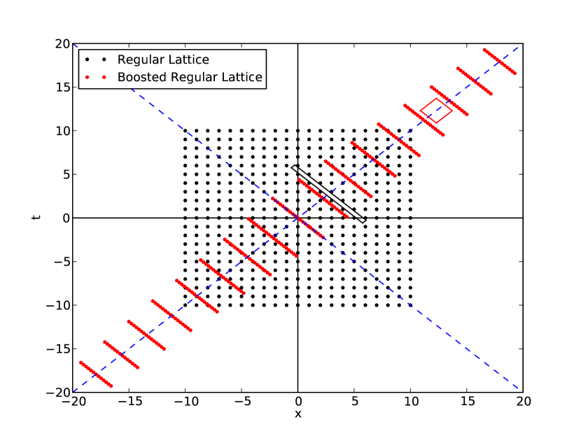
(a)

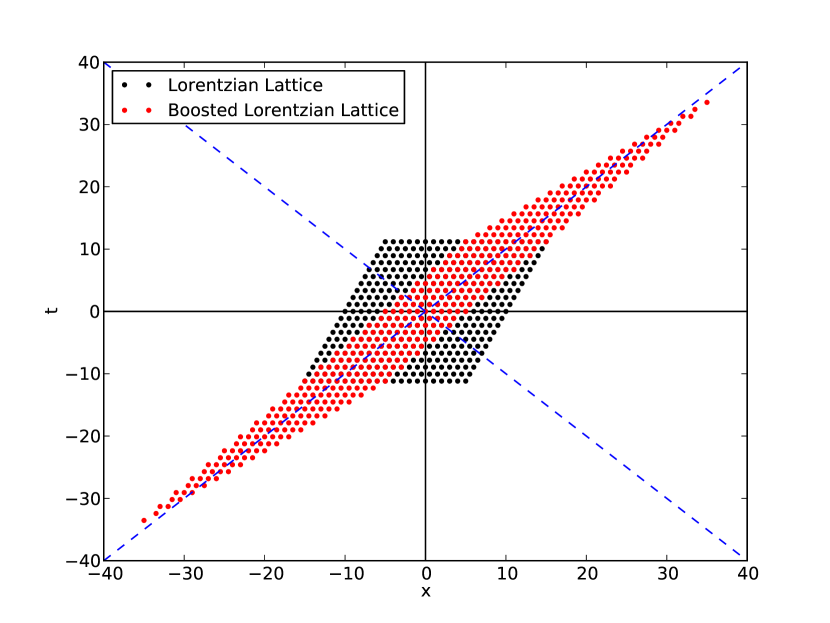
(b)

Figure 1: (a) The black dots show a lattice on the integers. The red dots are an active boost of this lattice by velocity $v=\tanh(1.5)$. The red diamond is a causal interval in the boosted frame which contains no points. The black diamond is the same causal interval as seen in the original frame. (b) The black dots show a Lorentzian lattice generated by the timelike vector $\xi_{(0)}=(\sqrt{5}/2,1/2)$, and the spacelike vector $\xi_{(1)}=(0,1)$. The red dots are boosts of the Lorentzian lattice by $v=\sqrt{5}/3$, showing that this particular boost takes the lattice to itself.

Are there any regular lattices in $1+1$ that do not have this problem? As it turns out, the answer is yes: Lorentzian lattices. These are lattices which are invariant under a discrete subgroup of the Lorentz group. Such a lattice is shown in Figure 1(b): it goes to itself under the action of a discrete set of boosts. We have classified all 2D Lorentzian lattices in Appendix B. In the case of the integer lattice shown in Figure 1(a), the more it is boosted, the more irregular it becomes. A Lorentzian lattice, however, does not have this problem because it eventually goes to itself. It is then reasonable to expect a better number-volume correspondence in this case.

We have investigated the $N$-$V$ correspondence for various Lorentzian lattices using simulations. Figure 2 shows the result of one such analysis on the lattice shown in Figure1(b). The setup is as follows: we consider $1000$ different causal diamonds with the same volume $V$, whose centres and shapes vary randomly throughout the lattice. For each realization, the number of lattice points inside the causal diamond is counted, leading to a distribution of the number of points for a given volume $V$. This procedure is then repeated for different volumes. As it can be seen from Figure 2, the Lorentzian lattice shown in Figure 1(b) realizes the number-volume correspondence with much less noise than Poisson sprinkling for macroscopic volumes. In fact, Figure 2(b) shows that the dispersion about the mean is barely growing with volume at all. The same exercise with the integer lattice results in a huge dispersion, much larger than that of Poisson, which is to be expected.

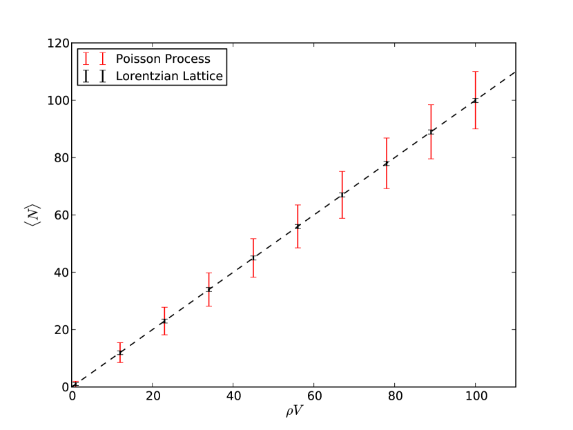
(a)

(b)

Figure 2: The number-volume correspondence for the Lorentzian lattice shown in Figure 1(b). (a) The mean and standard deviation of the number of points. (b) The histogram of the number of points for different volumes.

What about Lorentzian lattices in $3+1$ dimensions? Would they also realize the number-volume correspondence better than Poisson sprinkling? What is quite surprising is that the integer lattice is a Lorentzian lattice in both $2+1$ and $3+1$ dimensions Schild . We know from the $1+1$-dimensional integer lattice, however, that a boost along any spatial coordinate direction would create huge voids in any higher-dimensional integer lattice. Therefore, one would expect a poor number-volume realization in this case. We have confirmed this intuition for the $2+1$-dimensional integer lattice using simulations similar to those discussed previously (see Figure 3). What makes $1+1$-dimensional Minkowski space special is that boosts can only be performed along one direction. Therefore, a Lorentzian lattice does not “change” too drastically under the action of an arbitrary boost. This feature does not seem to persist in higher dimensions, which leads us to conclude that Lorentzian lattices in higher dimensions are not likely to realize the number-volume correspondence better than Poisson sprinkling.

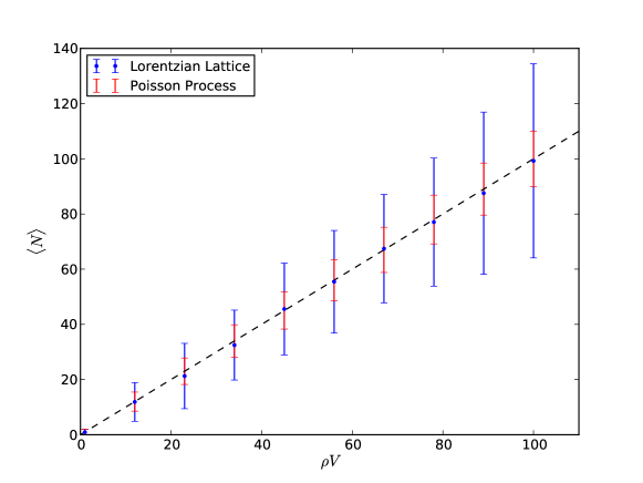
Figure 3: The number-volume correspondence for the $2+1$-dimensional integer lattice. For a given volume $V$, $200$ different causal diamonds with the same volume $V$ but randomly varying shapes are considered. The mean and standard deviation of the number of points (blue) is compared with that of the Poisson process (red).

4 A Conjecture

Based on the results of the previous Sections, we conjecture the following:

Conjecture 1.

Let $\xi$ be a point process whose realizations are points of a $3+1$-dimensional smooth Lorentzian manifold $(M,g)$. Let $N_{S}$ be the random variable which counts the number of points in a causal interval $S\subset M$: it takes on a value $n\in\{0,1,2,\dots\}$ with probability $P_{S}(n)$. Assume also that $\xi$ realizes the number-volume correspondence on average $\forall$ $S$: $\langle N_{S}\rangle=V_{S}$, where $V_{S}$ is the spacetime volume of $S$. Then, $\nexists$ $\xi$ and $V_{*}>0$ such that for all causal intervals $S$ with volume $V_{S}>V_{*}$:

$$\langle(N_{S}-V_{S})^{2}\rangle\leq\alpha V_{S}\quad\text{where}\qquad 0\leq\alpha<1.$$ (8)

5 Conclusions

Causal set theory maintains that all information about the continuum spacetime of general relativity is contained microscopically in a partially order and locally finite set. Discreteness allows one to count elements, which is thought to provide information about scale: a spacetime region with volume $V$ should contain about $\rho V$ causal set elements. In this paper, we proved a theorem which shows that this number-volume correspondence is best realized via Poisson sprinkling for arbitrarily small volumes. Quite surprisingly, we also showed that $1+1$-dimensional Lorentzian lattices provide a much better number-volume correspondence than Poisson sprinkling for large volumes. We presented evidence, however, that this feature should not persist in $3+1$ dimensions and conjectured that the Poisson process should indeed provide the best number-volume correspondence for macroscopically large spacetime regions.

Appendix A Proof of Inequality (6)

Theorem 2.

Let $N_{V}$ be a discrete random variable which takes on a value $n\in\{0,1,2,\cdots\}$ with probability $P_{V}(n)$, and whose mean is $V>0$:

$$\langle N_{V}\rangle=\sum_{n=0}^{\infty}nP_{V}(n)=V.$$ (9)

$N_{V}$ has the least variance when $P_{V}(n)=0$ $\forall$ $n\neq n_{*},n_{*}+1$, where $n_{*}$ is the largest integer which is smaller than or equal to $V$. Equivalently:

$$\langle(N_{V}-V)^{2}\rangle\geq(V-n_{*})(n_{*}+1-V),$$ (10)

where the inequality is saturated for the aforementioned process.

Proof.

The following three conditions must be true

$$\sum_{n=0}^{\infty}P_{V}(n) =1,$$ (11)

$$\sum_{n=0}^{\infty}P_{V}(n)n =V,$$ (12)

$$\ 0\leq P_{V}(n) \leq 1\qquad\forall\qquad n.$$ (13)

We denote the random variable which we claim has the least variance by $N^{m}_{V}$, and its probability mass function by $P^{m}_{V}$. It follows from (11) and (12) that

$$P^{m}_{V}(n_{*})=n_{*}+1-V,\qquad P^{m}_{V}(n_{*}+1)=V-n_{*},\qquad\langle(N^{m}_{V}-V)^{2}\rangle=(V-n_{*})(n_{*}+1-V).$$ (14)

Let us now show that for any other probability mass function $P_{V}(n)$:

$$\sigma_{V}^{2}\equiv\sum_{n=0}^{\infty}P_{V}(n)(n-V)^{2}\geq(V-n_{*})(n_{*}+1-V).$$ (15)

To this end, we define the following

$$A_{V} \equiv\sum_{n=0}^{n_{*}}P_{V}(n),$$ (16)

$$B_{V} \equiv\sum_{n=0}^{n_{*}}P_{V}(n)(V-n)=\sum_{n=n_{*}+1}^{\infty}P_{V}(n)(n-V),$$ (17)

where the last equality follows from (12). On the one hand,

$$B_{V}=\sum_{n=0}^{n_{*}}P_{V}(n)(V-n)\geq(V-n_{*})\sum_{n=0}^{n_{*}}P_{V}(n)=A_{V}(V-n_{*}).$$ (18)

On the other hand,

$$B_{V}=\sum_{n=n_{*}+1}^{\infty}P_{V}(n)(n-V)\geq(n_{*}+1-V)\sum_{n=n_{*}+1}^{\infty}P_{V}(n)=(n_{*}+1-V)(1-A_{V}).$$ (19)

It then follows from (18) and (19) that

$$1-\frac{B_{V}}{n_{*}+1-V}\leq A_{V}\leq\frac{B_{V}}{V-n_{*}},$$ (20)

which in turn implies that

$$B_{V}\geq(V-n_{*})(n_{*}+1-V).$$ (21)

Consider now the variance:

$$\sigma_{V}^{2} =\sum_{n=0}^{n_{*}-1}P_{V}(n)(n-V)^{2}+\sum_{n=n_{*}+2}^{\infty}P_{V}(n)(n-V)^{2}$$

$$+P_{V}(n_{*})(V-n_{*})^{2}+P_{V}(n_{*}+1)(n_{*}+1-V)^{2}.$$ (22)

For all $n\neq n_{*},n_{*}+1$, $(n-V)^{2}>|V-n|$, from which it follows that

$$\sigma_{V}^{2} \geq\sum_{n=0}^{n_{*}-1}P_{V}(n)(V-n)+\sum_{n=n_{*}+2}^{\infty}P_{V}(n)(n-V)$$

$$+P_{V}(n_{*})(V-n_{*})^{2}+P_{V}(n_{*}+1)(n_{*}+1-V)^{2}$$ (23)

$$=2B_{V}+(n_{*}-V)(n_{*}+1-V)\left[P_{V}(n_{*})+P_{V}(n_{*}+1)\right].$$ (24)

The equality in the last line follows from recognizing that

$$\sum_{n=n_{*}+2}^{\infty}P_{V}(n)(n-V)=\sum_{n=0}^{n_{*}+1}P_{V}(n)(V-n).$$ (25)

Finally, using the inequality (21):

$$\sigma_{V}^{2} \geq 2(V-n_{*})(n_{*}+1-V)+(n_{*}-V)(n_{*}+1-V)\left[P_{V}(n_{*})+P_{V}(n_{*}+1)\right]$$ (26)

$$=(V-n_{*})(n_{*}+1-V)\left[2-P_{V}(n_{*})-P_{V}(n_{*}+1)\right]$$ (27)

$$\geq(V-n_{*})(n_{*}+1-V),$$ (28)

where the last inequality follows from the fact that $P_{V}(n_{*})+P_{V}(n_{*}+1)\leq 1$. This concludes the proof of the theorem. ∎

Appendix B 2D Lorentzian Lattices: Details

We wish to construct a lattice that is invariant under the action of a discrete subgroup of the Lorentz group. We shall work in $D$-dimensional Minkowski space and use the metric signature $-++\cdots$. Consider $D$ vectors $\xi_{(d)}$, with $d\in\{0,1,2,\cdots,D-1\}$, which generate the lattice. In other words, any element of the lattice $X$ can be written as

$$X=n^{(d)}\xi_{(d)},$$ (29)

where $n^{(d)}$ are integers and the summation over $d$ is implicit. Let $\Lambda$ be an element of the Lorentz group. We require that for all points $X$ on the lattice, $\Lambda X$ is also a point on the lattice:

$$\Lambda X=n^{(d)}\Lambda\xi_{(d)}=m^{(d)}\xi_{(d)},$$ (30)

where $m^{(d)}$ are integers. We may decompose $\Lambda\xi_{(d)}$ in the basis of the generators:

$$\Lambda\xi_{(d)}=A_{(d)}^{\phantom{(d)}(d^{\prime})}\xi_{(d^{\prime})},$$ (31)

where $A_{(d)}^{\phantom{(d)}(d^{\prime})}$ are constants which depend on $\Lambda$ and $\xi_{(d)}$. It then follows from (30) that

$$n^{(d)}A_{(d)}^{\phantom{(d)}(d^{\prime})}=m^{(d^{\prime})}.$$ (32)

Therefore, $A_{(d)}^{\phantom{(d)}(d^{\prime})}$ must be an integer for all $d$ and $d^{\prime}$ if our lattice is to be invariant under the action of $\Lambda$. In order to compute $A$, we can“dot” both sides of (31) by $\xi_{(d^{\prime\prime})}$:

$$\Lambda\xi_{(d)}\cdot\xi_{(d^{\prime\prime})}=A_{(d)}^{\phantom{(d)}(d^{\prime})}\xi_{(d^{\prime})}\cdot\xi_{(d^{\prime\prime})}.$$ (33)

Defining the matrices $B$ and $C$ as,

$$B_{(d)}^{\phantom{(d)}(d^{\prime})}\equiv\xi_{(d)}\cdot\xi_{(d^{\prime})},\qquad C_{(d)}^{\phantom{(d)}(d^{\prime})}\equiv\Lambda\xi_{(d)}\cdot\xi_{(d^{\prime})},$$ (34)

it follows that

$$A=CB^{-1}.$$ (35)

Consider now the case of $1+1$ Minkowski space, i.e. $D=2$. Let $\xi_{(0)}$ and $\xi_{(1)}$ be the timelike and spacelike generators:

$$\xi_{(0)}=\epsilon\begin{pmatrix}\cosh\psi\\ \sinh\psi\end{pmatrix},\qquad\xi_{(1)}=\delta\begin{pmatrix}\sinh\theta\\ \cosh\theta\end{pmatrix},$$ (36)

where $\epsilon,\delta>0$. Also, since in $1+1$ we only have boosts to consider:

$$\Lambda=\begin{pmatrix}\cosh\phi&\sinh\phi\\ \sinh\phi&\cosh\phi\end{pmatrix}.$$ (37)

Defining the following quantities,

$$\gamma=\frac{\delta}{\epsilon},\qquad\chi=\psi-\theta,$$ (38)

it follows from (34) that

$$B=\epsilon^{2}\begin{pmatrix}-1&\gamma\sinh\chi\\ \gamma\sinh\chi&\gamma^{2}\end{pmatrix},\qquad C=\epsilon^{2}\begin{pmatrix}-\cosh\phi&\gamma\sinh(\phi+\chi)\\ \gamma\sinh(\chi-\phi)&\gamma^{2}\cosh\phi\end{pmatrix}.$$ (39)

Using (35):

$$A=\frac{1}{\cosh\chi}\begin{pmatrix}\cosh(\phi+\chi)&\frac{1}{\gamma}\sinh\phi\\ \gamma\sinh\phi&\cosh(\phi-\chi)\end{pmatrix}.$$ (40)

We need to pick $\phi,\chi$ and $\gamma$ so that all elements of $A$ are integers. Let $k_{1}-k_{4}$ be integers and require

$$\frac{\cosh(\phi+\chi)}{\cosh{\chi}}=k_{1},\qquad\frac{1}{\gamma}\frac{\sinh\phi}{\cosh{\chi}}=k_{2},\qquad\gamma\frac{\sinh\phi}{\cosh{\chi}}=k_{3},\qquad\frac{\cosh(\phi-\chi)}{\cosh{\chi}}=k_{4}.$$ (41)

Note that

$$k_{1},k_{4}>0,\qquad\text{sgn}(k_{2})=\text{sgn}(k_{3}).$$ (42)

The second and third equations in (41) are equivalent to

$$\gamma^{2}=\frac{k_{3}}{k_{2}},\qquad\frac{\sinh^{2}\phi}{\cosh^{2}\chi}=k_{2}k_{3}.$$ (43)

Also, the first and fourth equations in (41) imply

$$2\cosh\phi=k_{1}+k_{4},\qquad 2\sinh\phi\tanh\chi=k_{1}-k_{4}.$$ (44)

The first equation in (44) fixes $\phi$ up to a sign, using which the second equation in (43) fixes $\chi$ up to a sign. Putting these together in the second equation in (44), we obtain the following constraint on the integers $k_{1}-k_{4}$:

$$k_{1}k_{4}-k_{2}k_{3}=1.$$ (45)

This equation can be satisfied for various integers, and therefore there are many Lorentzian lattices in $1+1$.

To summarize: find integers $k_{1}-k_{4}$ that satisfy the conditions $(i)$ $k_{1},k_{4}>0$, $(ii)$ sgn($k_{2}$)=sgn($k_{3}$), (iii) $k_{1}k_{4}-k_{2}k_{3}=1$. Then, if we let $\cosh(\phi)=\frac{k_{1}+k_{4}}{2}$, $\gamma=\sqrt{k_{3}/k_{2}}$, and $\sinh(\chi)=\frac{k_{1}-k_{4}}{2\sqrt{k_{2}k_{3}}}$, the lattice generated by $\xi_{(0)}$ and $\xi_{(1)}$ goes to itself under the action of $\Lambda(\phi)$, with $\psi,\theta,\delta,\epsilon$ satisfying (38). Figure 1(b) shows an example of a Lorentzian lattice with $k_{1}=2$, $k_{2}=k_{3}=k_{4}=1$, $\delta=1$, and $\theta=0$.