Atomic Level Green-Kubo Stress Correlation Function for a Model Crystal:
An Insight into Molecular Dynamics Results on a Model Liquid.

Abstract

In order to get insight into the connection between the vibrational dynamics and the atomic level Green-Kubo stress correlation function in liquids we consider this connection in a model crystal instead. Of course, vibrational dynamics in liquids and crystals are quite different and it is not expected that the results obtained on a model crystal should be valid for liquids. However, these considerations provide a benchmark to which the results of the previous molecular dynamics simulations can be compared. Thus, assuming that vibrations are plane waves, we derive analytical expressions for the atomic level stress correlation functions in the classical limit and analyze them. These results provide, in particular, a recipe for analysis of the atomic level stress correlation functions in Fourier space and extraction of the wavevector and frequency dependent information. We also evaluate the energies of the atomic level stresses. Obtained energies are significantly smaller than the energies that were obtained in MD simulations of liquids previously. This result suggests that the average energies of the atomic level stresses in liquids and glasses are largely determined by the structural disorder. We discuss this result in the context of equipartition of the atomic level stress energies. Analysis of the previously published data suggests that it is possible to speak about configurational and vibrational contributions to the average energies of the atomic level stresses in a glass state. However, this separation in a liquid state is problematic. We also consider peak broadening in the pair distribution function with increase of distance. We find that peak broadening (by $\approx 40\%$) occurs due to the transverse vibrational modes, while contribution from the longitudinal modes does not change with distance. Finally, we introduce and consider atomic level transverse current correlation function.

I Introduction

In order to understand abrupt increase in viscosity of liquids approaching the glass transition, it is necessary to understand well the nature of viscosity itself. This understanding, however, is still limited HansenJP20061 ; EvansDJ19901 ; Boon19911 ; Hetero20131 ; Berthier2011 ; Tanaka20091 ; Tanaka2011E ; Levashov20111 ; Levashov2013 ; Iwashita2013 .

Computer simulations has proved to be an important tool in addressing properties of supercooled liquids HansenJP20061 ; EvansDJ19901 ; Boon19911 ; Hetero20131 ; Berthier2011 . One standard approach to calculate viscosity in computer simulations is based on the Green-Kubo expression that relates viscosity to the integral of the macroscopic stress correlation function HansenJP20061 ; EvansDJ19901 ; Boon19911 ; Green1954 ; Kubo1957 ; Helfand1960 ; EvansDJ19811 ; Hoheisel19881 .

Properties of the stress correlation function have been extensively studied previously from a macroscopic perspective HansenJP20061 ; EvansDJ19901 ; Boon19911 ; Hoheisel19881 . There have been significantly fewer studies that tried to address how behavior of the system at the atomic level translates into the macroscopic behavior of the stress correlation function Woodcock19911 ; Woodcock20062 ; Stassen19951 ; Stassen19952 ; Levashov20111 ; Levashov2013 ; Iwashita2013 .

The situation is similar with a closely related but somewhat different approach, i.e., the approach based on considerations of the transverse current correlation function HansenJP20061 ; EvansDJ19901 ; Boon19911 ; Tanaka20091 ; Tanaka2011E ; Tanaka20081 ; Mizuno2013 ; Mountain19821 . Studies of vibrational dynamics in disordered media with the transverse current correlation function are very common and several important results were obtained with it relatively recently Tanaka20091 ; Tanaka2011E ; Tanaka20081 . However, in all these studies the transverse current correlation function is treated as a macroscopic quantity. Thus the relations between the atomic level processes and the macroscopic behavior of the transverse current correlation function remain obscure Tanaka20091 ; Tanaka2011E .

We previously studied atomic level structure of the macroscopic Green-Kubo stress correlation function by decomposing it into correlation functions between the atomic level stresses Levashov20111 ; Levashov2013 . The approach represents further development of preceding works Hoheisel19881 ; Woodcock19911 ; Woodcock20062 ; Stassen19951 ; Stassen19952 . Our data clearly show presence of stress waves in the atomic level stress correlation function and that the stress waves contribute to viscosity Levashov20111 ; Levashov2013 . However, it was not previously discussed how stress waves and their properties translate into the observed atomic level stress correlation functions. It is difficult to address this issue in liquids, even qualitatively, as vibrational and configurational dynamics in liquids are mixed Stillinger20131 ; HeuerA20081 ; KeyesT19971 . Moreover, vibrational and configurational dynamics in disordered media are puzzles by themselves Stillinger20131 ; HeuerA20081 ; Zwanzig19651 ; KeyesT19971 ; Taraskin2000 ; Taraskin2002 ; Scopigno20071 ; Tanaka20081 ; Mizuno2013 ; Keys2011 ; Iwashita2013 ; Kob2006 ; Frenkel1947 ; Trachenko2009 ; Bolmatov2012 ; Bolmatov2013 .

On the other hand, as it appears from the review of the previous literature, the details of the connection between vibrational dynamics and the atomic level stress correlation function were not addressed previously even for those systems for which it could be done relatively easily, i.e., for the crystals. Applicability of results obtained from crystal models to liquids, in general, is not expected and should be considered with caution. However, it has been demonstrated that parallels between liquid and solid states can be useful Frenkel1947 ; Trachenko2009 ; Bolmatov2012 ; Bolmatov2013 .

Thus, in order to gain at least some qualitative or semiquantitative insight into the connection between the vibrational dynamics of a model liquid and the atomic level stress correlation functions observed in MD simulations Levashov20111 ; Levashov2013 , we examine a crystal-like model in which vibrations are represented by plane waves. Considerations in this paper represent further developments and more detailed discussions of some ideas and a model first presented in Ref.Egami19821 .

Another goal of this paper is to develop a framework for analysis in Fourier space of the MD data from a model liquid Levashov20111 ; Levashov2013 . This analysis is presented in Ref.Levashov20141 . It relies on the results presented in this paper.

To make derivations of the expressions for the stress correlation functions clearer it is useful to address several other issues. In particular, we calculate atomic level stress energies. In this context we discuss the data from previously published MD simulations on liquids and glasses Egami19821 ; Chen19881 ; Levashov2008B ; Levashov2008E .

In the framework of the model it is easy to evaluate the peak broadening in the pair distribution function with increasing distance. Calculations show that the peak broadening (by $\approx 40\%$) occurs because of the transverse waves, while the contribution from the longitudinal waves only weakly depends on distance.

Finally we briefly discuss the atomic level transverse current correlation function and argue that it is possible to study its behavior in MD simulations in a way which we previously applied to the atomic level stress correlation function.

The paper is organized as follows. In section II we describe the model. Section III is focused on derivations and analysis of the obtained results. In section IV we discuss obtained results in the broader context of some results obtained previously.

II The model

We consider a single component system and assume that different atoms have identical environments. In particular, we assume that every atom interacts harmonically with $N_{c}$ nearest neighbors. We also assume that distribution of these neighbors is spherically symmetric and that their equilibrium distance from the central atom is $a$. Finally we assume that vibrational motion in the system is described by plane waves.

II.1 Continuous spherical approximation

In the following derivations we will usually perform summation for every atom $n$ over its nearest neighbors $m$. In performing these summations we will utilize a continuous spherical approximation. Thus we will change summation over $m$ into the integration over the spherical angles:

$$\sum_{m}f(\theta_{m},\phi_{m})\rightarrow\frac{N_{c}}{4\pi}\int f(\theta,\phi)\sin(\theta)d\theta d\phi\;\;.\;\;\;\;\;\;\;\;$$ (1)

II.2 Debye’s Model

In order to estimate various quantities to which many different waves contribute we will assume that different waves contribute independently. We will also utilize Debye’s model, i.e., we will change summation over different waves into the integration over the wavevector:

$$\frac{dN}{N}=\left(\frac{a}{2\pi}\right)^{3}\,4\pi\,q^{2}\,dq\;\;,\;\;\;\;Q_{max}=\left(\frac{\pi}{a}\right)\left(\frac{6}{\pi}\right)^{1/3}\;\;,\;\;\;\;\;\;\;\;$$ (2)

where $N$ is the total number of atoms in the system and also the total number of vibrational states for one polarization. $dN$ is the number of states in the interval $dq$, and $Q_{max}$ is the maximum value of the wavevector. Equations in (2) are written for one particular polarization of the waves. We will assume further, as usual, that there are one longitudinal and two transverse polarizations.

The value of $Q_{max}$ and the value of the prefactor $\left(a/(2\pi)\right)^{3}$ in (2) are connected by the normalization condition. In principle, one can assume different values of $Q_{max}$ for different polarizations of the waves. We will not elaborate on this issue further.

II.3 Long wavelength approximation

In the following we will sometimes assume that:

$$\sin\left(\bm{q}\bm{a}_{nm}\right)\approx\left(\bm{q}\bm{a}_{nm}\right)\;\;,\;\;\;\cos\left(\bm{q}\bm{a}_{nm}\right)\approx 1\;\;.\;\;\;\;\;\;\;\;$$ (3)

Equations (3) are correct if the wavelength of the wave is much larger than the interatomic distance $a\equiv|\bm{a}_{nm}|$. Usually we will give the results obtained without long wavelength approximation and then, for comparison, the results obtained with long wavelength approximation.

III Derivations

III.1 Potential energy of an atom due to a plane wave

Let us assume that $\bm{r}_{n}^{o}$ is the equilibrium position of the particle $n$ and $\bm{u}_{n}$ is the displacement of the particle $n$ from equilibrium. Then $\bm{r}_{n}=\bm{r}_{n}^{o}+\bm{u}_{n}$, $r_{nm}=\left|\bm{r}_{m}-\bm{r}_{n}\right|$, $\bm{a}_{nm}=a\bm{\hat{a}}_{nm}=\left(\bm{r}_{m}^{o}-\bm{r}_{n}^{o}\right)$, $\bm{u}_{nm}=\bm{u}_{m}-\bm{u}_{n}$. With these notations potential energy for the nearest neighbor atoms $n$ and $m$ in the harmonic approximation is given by:

$$U_{nm}=\frac{k\left(r_{nm}-r_{nm}^{o}\right)^{2}}{2}\approx\frac{k}{2}\left(\bm{\hat{a}}_{nm}\bm{u}_{nm}\right)^{2}\;\;\;\;.$$ (4)

The solutions for particle displacements in classical harmonic crystals are plane waves. For a particular wave:

$$\bm{u}_{n}(\bm{q})=u_{q}\bm{\hat{e}}_{q}\,Re\left\{\chi_{n}(\bm{q})\right\}\;\;\;,\;\;\;$$ (5)

$$\chi_{n}(\bm{q})=\exp\left[-i\left(\omega_{\bm{q}}t-\bm{q}\bm{r}_{n}+\phi_{\bm{q}}\right)\right]\;\;\;,\;\;\;$$ (6)

where $u_{q}$ (real scalar) is the amplitude of the wave and $\bm{\hat{e}}_{q}$ (real vector) is its polarization vector.

From (5,6) we get:

$$\bm{u}_{nm}(\bm{q})=u_{q}\bm{\hat{e}}_{q}Re\left\{\chi_{n}(\bm{q})\left[\exp\left(i\bm{q}\bm{a}_{nm}\right)-1\right]\right\}\;\;.$$ (7)

It is straightforward to show from (4,7) that time average of the potential energy of the atom $n$ due to a particular wave is:

$$\left<U_{n}\right>_{t}\approx\left(\frac{1}{2}\right)\,ku_{q}^{2}\sum_{m}\left(\bm{\hat{a}}_{nm}\bm{\hat{e}}_{q}\right)^{2}\sin^{2}\left(\frac{\bm{q}\bm{a}_{nm}}{2}\right)\;\;,$$ (8)

where we introduced factor $1/2$ to take into account that half of the elastic energy belongs to the atom $n$, while another half to the atom $m$.

III.2 Force on an atom and dispersion relations

It follows from (4) that the force on the atom $n$ due to its interaction with the atom $m$ is:

$$f_{nm}^{\alpha}=-\frac{\partial U_{nm}}{\partial u_{n}^{\alpha}}=k(\bm{\hat{a}}_{nm}\bm{u}_{nm})\hat{a}_{nm}^{\alpha}\;\;.$$ (9)

Using the expression (7) for $\bm{u}_{nm}(\bm{q})$ in (9) for the total force on the atom $n$ we get:

$$f_{n}^{\alpha}= \sum_{m}(ku_{q})\,\left(\bm{\hat{a}}_{nm}\bm{\hat{e}}_{\bm{q}}\right)\,a_{nm}^{\alpha}\cdot$$

$$Re\left\{\chi_{n}(\bm{q})\left[\exp\left(i\bm{q}\bm{a}_{nm}\right)-1\right]\right\}\;\;\;\;.\;\;$$

Let us further suppose that we consider crystal lattices with central symmetry. Then for every neighbor $m$ there is another neighbor $m^{\prime}$ such that $\bm{a}_{nm^{\prime}}=-\bm{a}_{nm}$. This assumption should be true in the continuous spherical approximation. Taking this into account we can rewrite (III.2) as:

$$f_{n}^{\alpha}= \sum_{m}\left(ku_{q}\right)\left(\bm{\hat{a}}_{nm}\bm{\hat{e}}_{\bm{q}}\right)a_{nm}^{\alpha}\cdot$$

$$\left[\cos\left(\bm{q}\bm{a}_{nm}\right)-1\right]\cdot\cos\left(\omega_{\bm{q}}t-\bm{q}\bm{r}_{n}+\phi_{\bm{q}}\right)\;\;\;\;.\;\;\;\;$$

From (5,6,III.2) and Newton’s second law we get:

$$\hat{e}_{\bm{q}}^{\alpha}\omega_{L,T}^{2}(\bm{q})=\left(\frac{2k}{M}\right)\sum_{m}\left(\bm{\hat{a}}_{nm}\bm{\hat{e}}_{\bm{q}}\right)\sin^{2}\left(\frac{\bm{q}\bm{a}_{nm}}{2}\right)a_{nm}^{\alpha}\;\;,\;\;\;\;\;\;\;$$ (12)

where $M$ is the particle’s mass. Indexes $L$ and $T$ label longitudinal and transverse polarizations. Multiplication of both sides of (12) on $\hat{e}^{\alpha}_{\bm{q}}$ with the following summation over $\alpha$ leads to:

$$\omega_{L,T}^{2}(\bm{q})=\left(\frac{2k}{M}\right)\sum_{m}\left(\bm{\hat{a}}_{nm}\bm{\hat{e}}_{\bm{q}}\right)^{2}\sin^{2}\left(\frac{\bm{q}\bm{a}_{nm}}{2}\right).\;\;\;\;$$ (13)

Expression (13) is very similar to expression (8). This, of course, is not an occasion as the average potential energy of a site (8) due to a wave with the amplitude $u_{\bm{q}}$ should be equal to $M\omega^{2}_{\bm{q}}u^{2}_{\bm{q}}/4$.

Figure 1: Dispersion curves for the longitudinal and transverse waves in the continuous spherical approximation. Thick lines show the results obtained without the long wavelength approximation. Thin lines show the results obtained with the long wavelength approximation. Note that $\left(Q_{max}a\right)\cong 3.9$

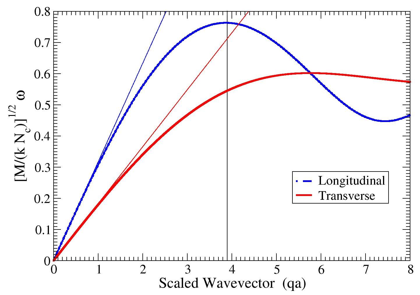
In the continuous spherical approximation (13) should not depend on the direction of $\bm{q}$ and an analytical expression for (13) could be obtained for the longitudinal and transverse waves. For a longitudinal wave it is sufficient to assume that $(\bm{q}\parallel\bm{\hat{z}})$ and $(\bm{\hat{e}_{q}}\parallel\bm{\hat{z}})$. For a transverse wave it is sufficient to assume that $(\bm{q}\parallel\bm{\hat{z}})$ and $(\bm{\hat{e}_{q}}\parallel\bm{\hat{x}})$. Thus we can rewrite (13) as:

$$\omega_{L,T}^{2}(q)=\omega_{o}^{2}D_{L,T}(qa)\equiv\frac{2}{4\pi}\int f_{L,T}(\xi,\theta,\phi)d\Omega\;\;\;,\;\;\;\;$$ (14)

where

$$\omega_{o}^{2}\equiv\left(\frac{k}{M}\right)N_{c}\;\;\;,\;\;\;\;\;\;\xi\equiv\frac{qa}{2}\;\;\;.\;\;$$ (15)

For longitudinal and transverse waves:

$$f_{L}(\xi,\theta,\phi)=\cos^{2}(\theta)\,\sin^{2}\left(\xi\cos(\theta)\right)\;\;\;,\;\;$$

$$f_{T}(qa,\theta,\phi)=\sin^{2}(\theta)\cos^{2}(\phi)\,\sin^{2}\left(\xi\cos(\theta)\right)\;\;\;.\;\;\;\;\;$$

Integrations over the spherical angles using the Maple(^TM) program Maple5 lead to:

$$D_{L}(qa)=\left[L_{1}(\xi)+L_{2}(\xi)\right]/\left[6\xi^{3}\right]\;\;\;,\;\;\;$$ (16)

$$D_{T}(qa)=\left[T_{1}(\xi)+T_{2}(\xi)\right]/\left[12\xi^{3}\right]\;\;\;,\;\;\;$$ (17)

where

$$L_{1}(\xi)=-6\,\xi^{2}\cos(\xi)\,\sin(\xi)+2\,\xi^{3}-6\,\xi\,\cos^{2}(\xi)\;\;\;,$$

$$L_{2}(\xi)=3\,\cos(\xi)\,\sin(\xi)+3\,\xi\;\;\;,$$

$$T_{1}(\xi)=4\xi^{3}+6\,\xi\,\cos^{2}(\xi)$$

$$T_{2}(\xi)=-3\,\cos(\xi)\,\sin(\xi)-3\,\xi\;\;\;.$$ (18)

The dependencies $\sqrt{D_{L}(qa)}$ and $\sqrt{D_{T}(qa)}$ on $qa$, i.e., the dispersion relations, are plotted in Fig.1.

The dispersion relations for the longitudinal and transverse waves could also be calculated in the long wavelength (lw) approximation:

$$\omega_{lw}^{2}(L,q)=\frac{\omega_{o}^{2}}{10}(qa)^{2},\;\;\;\;\;\omega_{lw}^{2}(T,q)=\frac{\omega_{o}^{2}}{30}(qa)^{2}.\;\;\;\;\;$$ (19)

Thus in the long wavelength approximation speeds of the longitudinal waves are $\sqrt{3}$ times larger than the speeds of the transverse waves.

III.3 Equipartition and mean square displacements

If we will assume that equipartition holds for our spherical approximation then the average potential energy of every wave should be equal to $k_{b}T/2$. Thus we should have:

$$\frac{M\omega_{L,T}^{2}(q)u_{L,T}^{2}(q)}{4}=\frac{1}{2}\frac{k_{b}T}{N}\;\;,$$

$$u_{L,T}^{2}(q)=2\left(\frac{k_{b}T}{kN_{c}}\right)\left(\frac{1}{D_{L,T}(qa)}\right)\frac{1}{N}\;\;,\;\;\;\;\;\;\;$$ (20)

where $u_{L,T}^{2}(q)$ is the average square amplitude of the longitudinal or transverse waves with the magnitude of the wave vector $q$. Thus the squares of the amplitudes are inversely proportional to the dispersion curves shown in the Fig.1. Note that wave’s amplitudes diverge for small wavevectors.

III.4 Mean square displacements due to all waves

In order to find the mean square displacements due to all waves, assuming that all of them are independent, we have to take half (since ($<u_{n}^{2}>=(1/2)u_{q}^{2}$) of (20) and integrate it over all $q$ using (2).

In this way for the mean square displacements due to all longitudinal waves and both polarizations of all transverse waves we get:

$$<u^{2}(L,T)>=\left(\frac{k_{b}T}{kN_{c}}\right)\gamma(L,T)\;\;,\;\;\;$$ (21)

$$\gamma(L)=2.8160\;\;,\;\;\;\;\;\gamma(T)=13.3615\;\;.\;\;\;$$

Note that $<u^{2}(T)>$ is significantly larger than $<u^{2}(L)>$.

It is simpler to evaluate the values of the mean square displacements in the long wavelength approximation. In this case we get:

$$\gamma_{lw}(L)=1.9746\;\;,\;\;\;\gamma_{lw}(T)=11.8478\$$ (22)

Note that the values of the coefficients in the long wavelength approximation are smaller than without the long wavelength approximations. This is consistent with (20), as the values of the frequencies are always larger in the long wavelength approximation.

III.5 The widths of peaks in the pair distribution function

Atoms located close to each other in the lattice should exhibit a certain degree of coherence in their motion. Because of this peaks in the pair distribution function at small distances should be narrower than at large distances. The dependence of the peak’s widths on distance was investigated previously using a detailed model and evolved simulations Chung1997 ; Chung1999 . It the frame of our model we can provide a simple evaluation of the size of the effect.

The average square of the peak width in the pair distribution function is determined by Chung1997 ; Chung1999 :

$$\left<\left(\Delta r_{nm}\right)^{2}\right>\cong\left<\left(\bm{\hat{r}}_{nm}^{o}\bm{u}_{nm}\right)^{2}\right>\;\;\;.\;\;\;$$ (23)

In (23) the notation $\left<...\right>$ is used for the time and spherical averages. Expression for $\left<\left(\Delta r_{nm}\right)^{2}\right>$ is completely analogous to the expression (4), but with $\bm{r}_{nm}^{o}$ instead of $\bm{a}_{nm}$.

In analogy with (4,8) and using the expression (20) for $u_{\bm{q}}^{2}$ we get:

$$\frac{k\left<\left(\Delta r_{nm}(\bm{q}\right)^{2}\right>}{2k_{b}T}\cong\frac{\sum_{m}\left(\bm{\hat{r}}_{nm}\bm{\hat{e}}_{\bm{q}}\right)^{2}\sin^{2}\left(\frac{\bm{q}\bm{r}_{nm}}{2}\right)}{\sum_{m}\left(\bm{\hat{a}}_{nm}\bm{\hat{e}}_{\bm{q}}\right)^{2}\sin^{2}\left(\frac{\bm{q}\bm{a}_{nm}}{2}\right)}\;\;\;\;\;\;$$ (24)

In order to estimate the peak width due to all waves it is necessary to integrate the numerator and denominator of (24) over the spherical angles and then their ratio over all $q$ using (2). The results of these integrations (assuming that $N_{c}=1$) for all longitudinal waves and one polarization of all transverse waves are shown in Fig.2.

Figure 2: The value of the ratio of sums in (24) integrated over all wavevectors as a function of $r$. The blue curve represents contributions from all longitudinal waves. The red curve represents contributions from one polarization of all transverse waves.

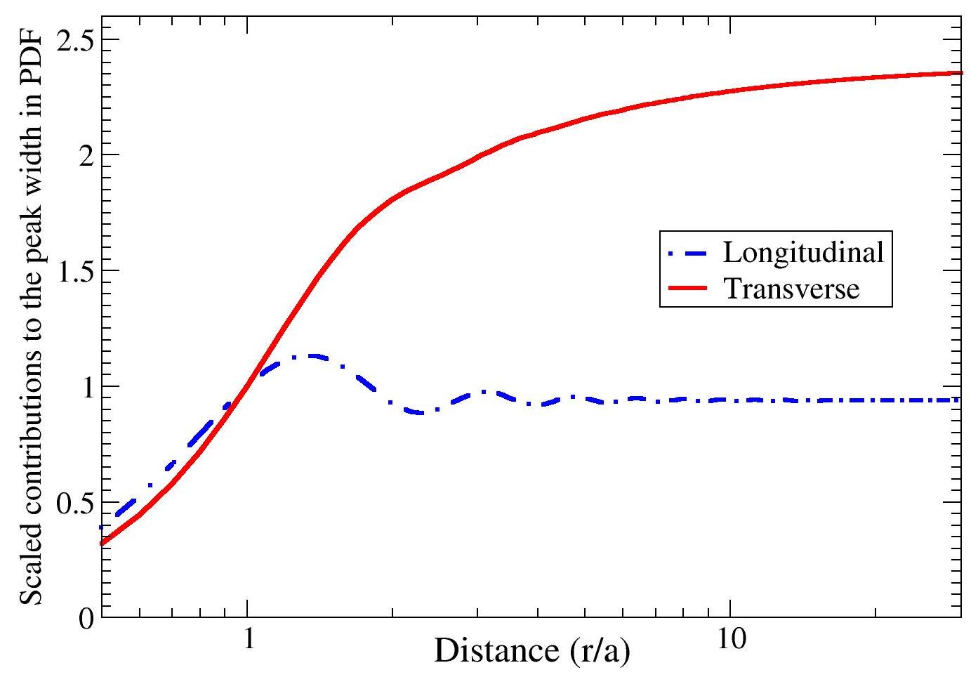
For large $r_{nm}$ motions of the atoms $n$ and $m$ should be uncorrelated. It is straightforward to show from (23) that if atoms $n$ and $m$ vibrate independently then $<(\Delta r_{nm})^{2}>=(2/3)<(u_{n})^{2}>$. This should be the large $r_{nm}$ limit of the peak’s width. In order to get this limit from the curves in Fig.2 it is necessary to multiply the limiting value by 2 for the longitudinal waves (the prefactor in 24) and by 4 for the transverse waves (the prefactor and two polarizations). Then the results can be compared with (21).

It is interesting that convergence to the final value for the transverse waves is slower than for the longitudinal waves. Note also that contribution to the peak width from the shear waves increases by more than twice as the distance increases. There is essentially no change in the peak’s widths with distance due to the longitudinal waves.

III.6 Atomic level stress elements

Similarly to the previous definitions Egami19821 ; Chen19881 ; Levashov2008B , we define the $\alpha\beta$-component of the local atomic stress element on a particle $n$ as:

$$s_{n}^{\alpha\beta}=\frac{1}{2}\sum_{m\neq n}f_{nm}^{\alpha}r_{nm}^{\beta}\;\;,$$ (25)

where, $f_{nm}^{\alpha}$ is the $\alpha$-component of the force on the particle $n$ caused by the interaction with the particle $m$ and $r_{nm}^{\beta}$ is the $\beta$-component of the radius vector from the particle $n$ to the particle $m$. The sign in (25) was chosen in such a way that an atom under compression will have a negative stress/pressure.

If there are interactions between the nearest neighbors only, we can rewrite (25) using (9) as:

$$s_{n}^{\alpha\beta}=\frac{\left(ka\right)}{2}\sum_{m\neq n}(\bm{u}_{nm}\bm{\hat{a}}_{nm})\hat{a}_{nm}^{\alpha}\hat{a}_{nm}^{\beta}\;\;,$$ (26)

Using (7) in (26) for the complex stress we obtain:

$$s_{n}^{\alpha\beta}(\bm{q})=\frac{\left(ka\right)}{2}u_{\bm{q}}\chi_{n}(\bm{q})\cdot$$

$$\cdot\sum_{m\neq n}\left(\bm{\hat{e}_{q}}\bm{\hat{a}}_{nm}\right)\left[\exp\left(i\bm{q}\bm{a}_{nm}\right)-1\right]\hat{a}_{nm}^{\alpha}\hat{a}_{nm}^{\beta}\;\;\;.\;\;\;\;$$ (27)

Let us, like in the transition from (III.2) to (III.2), again assume that we consider crystal lattices with the central symmetry. For the real part of the stress from (27) we get:

$$s_{n}^{\alpha\beta}(\bm{q})=\frac{\left(kau_{q}\right)}{2}N_{c}\Upsilon^{\alpha\beta}_{1}\left(\bm{q},\bm{\hat{e}}_{q}\right)\sin\left(\omega_{\bm{q}}t-\bm{q}\bm{r}_{n}+\phi_{\bm{q}}\right)\;,\;\;\;\;\;\;\;\;$$ (28)

where

$$\Upsilon^{\alpha\beta}_{1}\left(\bm{q},\bm{\hat{e}}_{q}\right)\equiv\frac{1}{N_{c}}\sum_{m\neq n}\left(\bm{\hat{e}}_{\bm{q}}\bm{\hat{a}}_{nm}\right)\sin\left(\bm{q}\bm{a}_{nm}\right)\hat{a}_{nm}^{\alpha}\hat{a}_{nm}^{\beta}\;\;.\;\;\;\;\;\;\;\;$$ (29)

Formulas (28,29) express local atomic stress elements due to a particular wave through the parameters of the lattice and the parameters of the propagating wave.

III.7 Atomic level pressure

In accord with Egami19821 ; Chen19881 ; Levashov2008B , we define atomic level pressure as:

$$p_{n}(\bm{q})=\frac{1}{3v_{o}}\left[s^{xx}_{n}(\bm{q})+s^{yy}_{n}(\bm{q})+s^{zz}_{n}(\bm{q})\right]\;\;\;,\;\;\;\;$$ (30)

where $v_{o}$ is atomic volume. Here we will assume that atomic volume is a constant approximately equal to the inverse of the number density, i.e., $v_{o}\approx 1/\rho_{o}$.

It follows from (28,29,30) that:

$$p_{n}(\bm{q})=\frac{\left(kau_{q}\right)N_{c}}{6v_{o}}\Upsilon^{p}_{1}\left(\bm{q},\bm{\hat{e}}_{q}\right)\sin\left(\omega_{\bm{q}}t-\bm{q}\bm{r}_{n}+\phi_{\bm{q}}\right)\;\;,\;\;\;\;\;\;$$ (31)

where

$$\Upsilon^{p}_{1}\left(\bm{q},\bm{\hat{e}}_{q}\right)=\frac{1}{N_{c}}\sum_{m\neq n}\left(\bm{\hat{e}}_{\bm{q}}\bm{\hat{a}}_{nm}\right)\sin\left(\bm{q}\bm{a}_{nm}\right)\;\;\;.\;\;\;\;$$ (32)

Summation over $m$ (spherical integration) for a longitudinal wave leads to:

$$\Upsilon^{p}_{1}\left(L,qa\right)=\left[\frac{\sin(2\xi)-(2\xi)\cos(2\xi)}{(2\xi)^{2}}\right],\;\;\;\xi=\frac{qa}{2}\;.\;\;\;$$ (33)

It also follows from (32) that transverse waves do not contribute to the pressure.

III.8 Mean square of the atomic level pressure

It follows from (31,32,35) that time averaged square of the pressure due to a longitudinal wave with the wavevector of magnitude $q$ is:

$$\left<\left[p_{n}(q)\right]^{2}\right>=\frac{\left(kau_{q}\right)^{2}N_{c}^{2}}{72v_{o}^{2}}\cdot\Upsilon^{p}_{2}\left(L,qa\right)\;\;\;,\;\;\;\;$$ (34)

where

$$\Upsilon^{p}_{2}\left(L,qa\right)\equiv\left[\Upsilon^{p}_{1}\left(L,qa\right)\right]^{2}\;\;.\;\;\;\;$$ (35)

In the long wavelength approximation:

$$\Upsilon^{p}_{2,lw}\left(L,qa\right)\approx\frac{1}{9}(qa)^{2}\;\;\;.\;\;\;$$ (36)

Expressing $u_{q}^{2}$ from (20) and then using it in (34) leads, after integration (2) over $q$, to:

$$\left<p_{n}^{2}\right>\approx k_{b}T\cdot\left(\frac{ka^{2}N_{c}}{36v_{o}^{2}}\right)\cdot 0.29\;\;\;\;.$$ (37)

Calculations in the long wavelength approximation lead to $\approx 1.11$ instead of $\approx 0.29$.

III.9 Atomic level pressure energy

In several previous publications atomic level stress energies were discussed Egami19821 ; Chen19881 ; Levashov2008B . These quantities are of interest, in particular, because of their values in the liquid states. According to MD simulations, the stress energy for every stress component is very close to $(1/4)k_{b}T=(1/6)(3/2)k_{b}T$.

It is well known that the average potential energy of a classical $3D$ harmonic oscillator is equal to $(3/2)k_{b}T$. Thus the values of the atomic levels stress energies are such that it appears that the average potential energy of some $3D$ harmonic oscillator is equally divided between the six independent components of the atomic level stresses. Thus it is interesting to estimate the values of the local atomic stress energies in our model.

The expression for the local atomic pressure energy is Egami19821 ; Levashov2008B :

$$<U^{p}>\equiv\frac{v_{o}\left<p_{n}^{2}\right>}{2B}\;\;\;\;.\;\;\;\;\;\;$$ (38)

In order to evaluate the expression we need to know the value of the bulk modulus $B$. The expressions for the elastic constants were discussed before Egami19821 ; Levashov2008B . The results of their evaluations are:

$$B=\frac{\varkappa}{8}\;\;,\;\;\;\;\;\;G=\frac{\varkappa}{30}\;\;,\;\;\;\;\;\;\varkappa=\left(ka^{2}\right)\frac{N_{c}}{v_{o}}\;\;,\;\;\;\;\;\;\;$$ (39)

where $G$ is the shear modulus. Using the value of the bulk modulus $B$ for the average pressure stress energy we get:

$$<U^{p}>\approx\left(\frac{1}{4}\right)k_{b}T\cdot\left(\frac{1}{7.76}\right)\;\;.$$ (40)

This energy is significantly smaller than the value of the pressure energy that was obtained for liquids.

In the long wavelength approximation we get:

$$<U^{p}_{lw}>\cong\left(\frac{1}{4}\right)k_{b}T\cdot\frac{1}{2.03}\;\;.$$ (41)

Thus in the long wavelength approximation the atomic level pressure stress energy is approximately 2 times smaller than the equipartition value, in agreement with Egami19821 . However, without the long wavelength approximation the local atomic pressure energy is more than 7 times smaller than the equipartition value. We address these differences further in the discussion section.

III.10 Pressure-pressure correlation function

Our goal here is to address the behavior of the atomic level stress correlation function that is analogous to the function $F(t,r)$ that could be derived from the macroscopic Green-Kubo stress correlation function and that was studied by MD simulations previously Levashov20111 ; Levashov2013 . Thus we introduce:

$$C^{p}(t,r)=\left(\frac{a}{2\pi}\right)^{3}N\int_{0}^{Q_{max}}C^{p}(t,r,q)\,4\pi q^{2}dq\;\;\;,\;\;\;\;$$ (42)

where

$$C^{p}(t,r,q)=\left<p_{n}(t_{o},q)\cdot p_{m}(t_{o}+t,q)\right>\;\;\;.\;\;\;\;$$ (43)

Spherical averaging and the averaging over $t_{o}$ are assumed in (43).

Note that the correlation function that we introduced in (42,43) is the correlation function per pair of particles and not the correlation function between “a central particle” and “the particles in the spherical annulus”, as it was done in Levashov20111 ; Levashov2013 .

Figure 3: Pressure-Pressure correlation function without long wavelength approximation.

Figure 4: Pressure-Pressure correlation function with long wavelength approximation.

From (31,32) it follows that:

$$C^{p}(t,r,q)=\frac{\left(kau_{q}\right)^{2}}{36v_{o}^{2}}\cdot\Upsilon^{p}_{2}\left(L,qa\right)\cdot\;\;\;\;\;\;\;\;\;$$ (44)

$$\left<\sin\left[\omega_{\bm{q}}t_{o}-\bm{q}\bm{r}_{n}+\phi_{\bm{q}}\right]\sin\left[\omega_{\bm{q}}(t_{o}+t)-\bm{q}\bm{r}_{m}+\phi_{\bm{q}}\right]\right>\;\;\;.\;\;\;\;$$

From representing the product of sines as a difference of cosines it follows that one of the cosines gives zero on averaging over $\phi_{\bm{q}}$. Thus we get:

$$C^{p}(t,r,q)=$$

$$\frac{\left(kau_{q}\right)^{2}}{36v_{o}^{2}}\cdot\Upsilon^{p}_{2}\left(L,qa\right)\cdot\frac{1}{2}\left<\cos\left[\frac{\omega_{\bm{q}}t-\bm{q}\bm{r}_{nm}}{2}\right]\right>$$ (45)

Further we rewrite $\cos\left[\frac{\omega_{\bm{q}}t-\bm{q}\bm{r}_{nm}}{2}\right]$ as:

$$\left<\cos\left[\frac{\omega_{\bm{q}}t}{2}\right]\cos\left[\frac{\bm{q}\bm{r}_{nm}}{2}\right]\right>+\left<\sin\left[\frac{\omega_{\bm{q}}t}{2}\right]\sin\left[\frac{\bm{q}\bm{r}_{nm}}{2}\right]\right>\;\;\;\;\;\;\;$$ (46)

Spherical averaging of the second term over the directions of $\bm{r}_{nm}$ is zero. Spherical averaging in the first term gives:

$$\left<\cos\left[\frac{\bm{q}\bm{r}_{nm}}{2}\right]\right>=2\frac{\sin\left(qr/2\right)}{(qr/2)}\;\;\;.$$ (47)

Using the expression (20) for $u_{q}^{2}$ we rewrite (45) as:

$$C^{p}(t,r,q)=k_{b}T\left(\frac{ka^{2}N_{c}}{v_{o}^{2}}\right)\cdot\frac{1}{36}\cdot$$

$$\cdot\frac{2}{N}\left\{\frac{\Upsilon^{p}_{2}\left(L,qa\right)}{D_{L}(qa)}\right\}\cdot\left\{\frac{\cos\left(\omega_{q}t/2\right)\sin\left(qr/2\right)}{(qr/2)}\right\}\;\;,\;\;\;\;\;$$ (48)

where, according to (14), $\omega_{q}=\omega_{o}\sqrt{D_{L}(qa)}$. The product of the cosine and sine in (48) could be rewritten as:

$$\frac{1}{2}\left[\sin\left(\frac{qr-\omega_{q}t}{2}\right)+\sin\left(\frac{qr+\omega_{q}t}{2}\right)\right]\;\;\;.\;\;\;\;\;\;$$ (49)

The first sine corresponds to a wave propagating from the central particle. This sine is zero when $r-(\omega_{\bm{q}}/q)t=0$. The argument of the second sine is always positive for positive $t$ and $r$. For positive times the contribution to the stress correlation function due to all waves from the second sine is much smaller than from the first sine. However, for negative times the second sine behaves like the first sine for positive times.

In order to find the pressure correlation function due to all waves we have to integrate (48) over all $q$ using (2). Fig.3 shows the results for the pressure-pressure correlation function due to all waves without long wavelength approximation. Fig.4 shows the result with long wavelength approximation.

III.11 An example of the local atomic shear stress and shear stress energy

In accord with references Egami19821 ; Chen19881 ; Levashov2008B we define:

$$\sigma^{\epsilon}_{n}(\bm{q},\bm{\hat{e}}_{\bm{q}})=\left(\frac{\sqrt{2}}{v_{o}}\right)s^{xy}_{n}(\bm{q},\bm{\hat{e}}_{\bm{q}})\;\;\;.\;\;\;\;\;$$ (50)

Both longitudinal and transverse waves contribute to $\sigma^{\epsilon}_{n}(\bm{q},\bm{\hat{e}}_{\bm{q}})$. Their contributions depend on the magnitude and direction of $\bm{q}$ and the direction of $\bm{\hat{e}}_{\bm{q}}$. Below, for shortness, we present the formulas for the transverse waves only. The formulas for the longitudinal waves are analogous.

From (28,29,50,20) we get:

$$\left<\left[\sigma^{\epsilon}_{n}(T,q)\right]^{2}\right>=\left(k_{b}T\right)\left(\frac{ka^{2}N_{c}}{2v_{o}^{2}}\right)\frac{1}{N}\left[\frac{\Upsilon^{xy}_{2}\left(T,qa\right)}{D_{T}\left(qa\right)}\right],\;\;\;\;\;$$ (51)

where:

$$\Upsilon^{xy}_{2}\left(T,qa\right)\equiv\left<\left[\Upsilon^{xy}_{1}\left(T,\bm{q},\bm{\hat{e}_{q}},a\right)\right]^{2}\right>\;,$$ (52)

and $\Upsilon^{xy}_{1}\left(T,\bm{q},\bm{\hat{e}_{q}},a\right)$ is given by (29). The averaging in (52) is over all directions of $\bm{\hat{e}}_{\bm{q}}$ orthogonal to $\bm{q}$ and then over the directions of $\bm{q}$.

We were not able to produce analytical expressions for $\Upsilon^{xy}_{2}\left(T,qa\right)$ and $\Upsilon^{xy}_{2}\left(L,qa\right)$. However, we calculated them numerically numerically . Fig.5 shows the dependencies of

$$H^{p}(L,qa)\equiv \left[\frac{\Upsilon^{p}_{2}(L,qa)}{D_{L}(qa)}\right](qa)^{2}\;\;\;,\;\;\;\;$$ (53)

$$H^{xy}(L,qa)\equiv \left[\frac{\Upsilon^{xy}_{2}(L,qa)}{D_{L}(qa)}\right](qa)^{2}\;\;\;,\;\;\;\;$$ (54)

$$H^{xy}(T,qa)\equiv \left[\frac{\Upsilon^{xy}_{2}(T,qa)}{D_{T}(qa)}\right](qa)^{2}\;$$ (55)

on $qa$ without long wavelength approximation. In (53,54,55) we introduced the factor $(qa)^{2}$ assuming further integrations over $q$.

We also obtained analytical expressions for (52) in the long wavelength approximation:

$$\frac{\Upsilon^{xy}_{2,lw}(L,qa)}{D_{L}(qa)}\approx\left[\frac{8}{675}\right],\;\;\;\;\;\frac{\Upsilon^{xy}_{2,lw}(T,qa)}{D_{T}(qa)}\approx\left[\frac{18}{675}\right].\;\;\;\;\;$$ (56)

Figure 5: Functions $H^{p}(L,qa)$, $H^{xy}(L,qa)$, and $H^{xy}(T,qa)$ from (53,54,55). Note that $H^{xy}(L,qa)$ curve was scaled by $100$, while $H^{xy}(T,qa)$ curve was scaled by $50$. Thus the contribution of the transverse waves to the average square of the shear stress is significantly larger than the contribution from the longitudinal waves. Also note that there are two polarizations of the transverse waves, while the figure shows the contribution from one polarization only.

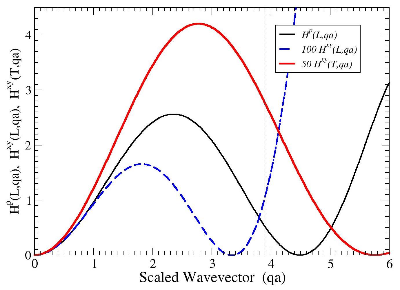
In order to evaluate mean square stresses due to all waves we have to integrate (51), i.e., the curves in Fig.5, over all $q$ using (2). The results of these integrations, expressed in terms of the average energy of the atomic level shear stresses, are:

$$\frac{v_{o}\left<\left[\sigma_{n}^{\epsilon}(L,T)\right]^{2}\right>}{4G}\approx\left(\frac{1}{4}\right)k_{b}T\cdot\tau(L,T)\;\;\;,\;\;\;$$ (57)

$$\tau(L)\approx\frac{3.1}{135},\;\;\;\;\;\tau(T)\approx\frac{20.6}{135}\;\;\;.\;\;\;$$

The shear stress energy coefficient due to all waves is:

$$\tau(L)+2\tau(T)\approx(44.3/135)\approx\frac{1}{3}\;\;\;.\;\;$$ (58)

Thus we got the result which is 3 times smaller than the equipartition result for certain MD liquids Chen19881 ; Levashov2008B . Also note that this result is more than two times larger than the result that was obtained for the pressure (40).

In the long wavelength approximation we get:

$$\tau_{lw}(L)=\frac{24}{135},\;\;\;\;\;\;\;\;\;\tau_{lw}(T)=\frac{54}{135},\;\;\;$$ (59)

$$\tau_{lw}(L)+2\tau_{lw}(T)=(132/135)\approx 1\;.\;\;\;$$ (60)

Thus in the long wavelength approximation we essentially have $(1/4)k_{b}T$ dependence.

III.12 Shear Stress Correlation Function

In order to introduce a shear stress correlation function which is analogous to the function $F(t,r)$ in Levashov20111 ; Levashov2013 we first introduce a correlation function due to a particular wave. For a particular transverse wave we write:

$$C^{\epsilon}_{\bm{q}}(T,t,r,\bm{q},\bm{\hat{e}_{q}})=\left(\frac{2}{v_{o}^{2}}\right)\cdot$$ (61)

$$\left<s_{n}^{xy}(t_{o},\bm{q},\bm{\hat{e}_{q}})\cdot s_{m}^{xy}(t_{o}+t,\bm{q},\bm{\hat{e}_{q}})\right>=$$ (62)

$$\left(k_{b}T\right)\left(\frac{ka^{2}N_{c}}{2v_{o}^{2}}\right)\frac{1}{N}\left[\frac{\left(\Upsilon^{xy}_{1}\left(T,\bm{q},\bm{\hat{e}_{q}},a\right)\right)^{2}}{D_{T}\left(qa\right)}\right]\cdot$$ (63)

$$\left<\sin\left[\omega_{\bm{q}}t_{o}-\bm{q}\bm{r}_{n}+\phi_{\bm{q}}\right]\sin\left[\omega_{\bm{q}}(t_{o}+t)-\bm{q}\bm{r}_{m}+\phi_{\bm{q}}\right]\right>\;.\;\;\;\;\;\;\;\;$$ (64)

Similarly to how it was done in the transition from (III.10) to (48) for the pressure-pressure correlation function we now average over the different directions of $\bm{r}_{nm}$. The difference with the pressure-pressure case is that now the prefactor depends on the direction and the polarization of the wave, while in the pressure-pressure case it depends only on the magnitude of the wavevector. This difference is, however, irrelevant for the averaging over the directions of $\bm{r}_{nm}$. Then we perform the averaging over the polarization and the direction of the wave. This averaging is identical to the averaging that was done in derivations of (51,52). Thus we get:

$$C^{\epsilon}(T,t,r)=\left(\frac{a}{2\pi}\right)^{3}N\int_{0}^{Q_{max}}C^{\epsilon}(T,t,r,q)\,4\pi q^{2}dq\;,\;\;\;\;\;\;\;$$ (65)

where

$$C^{\epsilon}(T,t,r,q)=k_{b}T\left(\frac{ka^{2}N_{c}}{v_{o}^{2}}\right)\cdot E(\omega_{q}t)\cdot$$

$$\cdot\frac{2}{N}\left\{\frac{\Upsilon^{xy}_{2}\left(T,qa\right)}{D_{T}(qa)}\right\}\cdot\left\{\frac{\cos\left(\omega_{q}t/2\right)\sin\left(qr/2\right)}{(qr/2)}\right\}\;\;\;.\;\;\;\;$$ (66)

In (66) we introduced the function $E(\omega_{q}t)$ artificially. It should not be there if the waves do not decay with time or distance. However, if we want to make a comparison with the stress correlation functions calculated in MD simulations on liquids, then it is reasonable to assume that waves decay. For the sake of a qualitative comparison we assume that Mizuno2013 :

$$E(\omega_{q},t)=\exp\left[-0.3(\omega_{q}/\omega_{o})^{2}\omega_{o}t\right]\;\;\;.\;\;\;$$ (67)

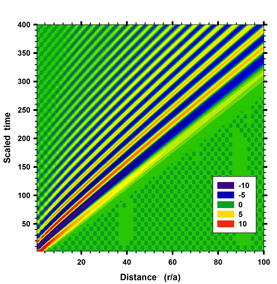
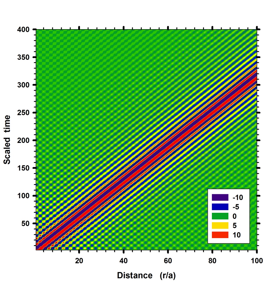
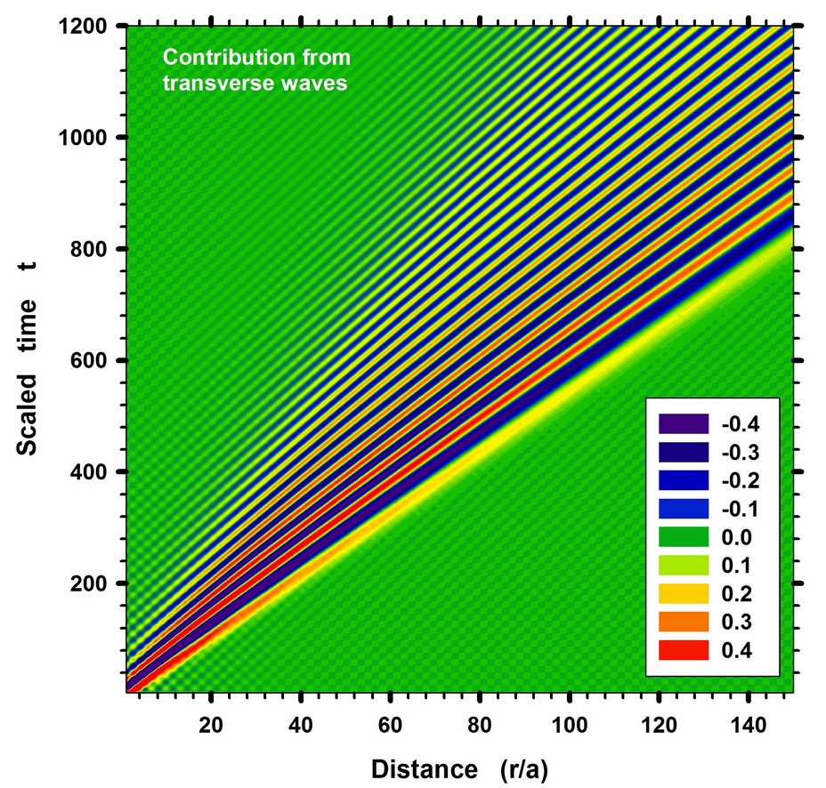
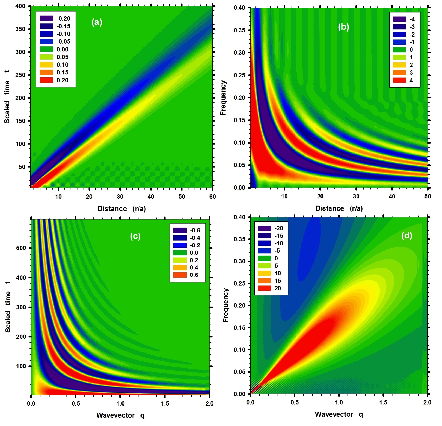
Figure 6 shows the stress correlation function calculated numerically from (65,66) under the assumption that the first row in (66) is equal to 1. Panel (a) of Figure 7 again shows the stress correlation function (65,66), but now with $E(\omega_{q},t)$ given by (67). We do not show in the figure the contribution from the longitudinal waves. This contribution is qualitatively similar to the contribution from the transverse waves. However, this contribution is significantly smaller in magnitude. Also, since the speeds of the longitudinal waves are $\approx\sqrt{3}$ times larger than the speeds of the transverse waves, the diagonal lines in the contribution from the longitudinal waves have slopes which are $\approx\sqrt{3}$ times smaller than the slopes of the diagonal lines from the transverse waves.

It is interesting to compare the panel (a) of Fig.7 with the panel (b) of Fig.4 in Ref.Levashov2013 . Note that in the present paper we changed the axes and now $x$-axis shows the distance, while $y$-axis shows the time. In the panel (b) of Fig.4 in Ref. Levashov2013 we see two waves. One wave is longitudinal and another wave is transverse. There we also see pdf - like contribution to the stress correlation function. In the panel (a) of Fig.7 we see the contribution from the transverse waves only, since we did not include in it the contribution from the longitudinal waves or the pdf - like structure. Besides the differences mentioned above, it is clear that the contribution to the stress correlation function from the transverse waves observed in MD simulation and in the present calculations are qualitatively similar. In particular, if we consider how intensity changes with increase of time for a given distance we observe at first positive intensity and then negative intensity.

Formula (49) suggests that the speed of the wave corresponds to the slope of the first boundary between the positive and negative intensities. This interpretation is different from the one adopted in Ref.Levashov2013 . There it was assumed that the center of the wave corresponds to the maximum of the positive intensity. With the new interpretation the speed of the longitudinal waves in the panel (b) of Fig.4 in Ref. Levashov2013 is $c_{l}\approx 7500$ (m/s) while before it was argued that it is 6000 (m/s). The new speed of the transverse waves is $c_{t}\approx 5000$ (m/s), while before it was argued that it is 3000 (m/s). Note that, according to the new values, $c_{l}/c_{t}\approx 1.5$, which is not quite $\sqrt{3}$.

Figure 6: Contribution from one polarization of the transverse waves to the shear stress correlation function. Scaled time is $\omega_{o}t$. No damping of the waves is assumed.

III.13 Fourier transforms of the shear stress correlation function

The atomic level stress correlation functions, like those in (48,66), could be calculated in MD simulations Levashov20111 ; Levashov2013 . In this section we analyze what information could be obtained by performing Fourier transforms of these stress correlation functions (48,66). Thus further we consider a function which is structurally similar to the stress correlation functions (48,66):

$$f(t,r)\equiv\int_{0}^{Q_{max}}h(q,t)\cos\left(\frac{\omega_{q}t}{2}\right)\sin\left(\frac{qr}{2}\right)dq\;\;\;.\;\;\;\;\;\;$$ (68)

For the shear stress correlation function due to the transverse waves (66), for example, we have:

$$f(t,r)\equiv r\cdot C^{\epsilon}(T,t,r)\;\;\;,\;\;\;$$ (69)

$$h(q,t)\equiv\alpha\left(\frac{Y_{2}^{xy}(T,q)}{D_{T}(qa)}\right)\cdot E(\omega_{q},t)\cdot q\;\;\;,\;\;\;$$ (70)

where $\alpha$ is a numerical coefficient. Note that $f(t,r)$, as we define it, is the correlation function per pair of particles multiplied by $r$.

Further we define:

$$\tilde{f}(t,q)\equiv\int_{0}^{\infty}f(t,r)\,\sin(qr)dr\;\;\;,\;\;\;$$ (71)

$$\tilde{f}(\omega,r)\equiv\int_{0}^{\infty}f(t,r)\,\cos(\omega\,t)dt\;\;\;,\;\;\;$$ (72)

$$\tilde{f}(\omega,q)\equiv\int_{0}^{\infty}\int_{0}^{\infty}f(t,r)\,\cos(\omega\,t)\,\sin(qr)\,dt\,dr\;\;\;.\;\;\;\;\;$$ (73)

From (71,68,70) we get:

$$\tilde{f}(t,q)\equiv\left(\frac{\pi}{2}\right)h(2q,t)\cos\left(\frac{\omega_{2q}t}{2}\right)\;\;\;\;,\;\;\;\;$$ (74)

where $\omega_{2q}^{2}=\omega_{o}^{2}D_{T}(2qa)$. Thus $\tilde{f}(t,q)$, for every value of $q$, oscillates in time with the period determined by the dispersion relation. The decrease in the amplitude of oscillations with increase of time is determined by the damping function $E(\omega_{q},t)$ (70). If there were no damping function the amplitude of oscillations would remain constant.

The situation with the Fourier transform of $f(t,r)$ over time is more complicated. In general, for liquids the damping function is not exponential, but a function that describes different relaxation regimes. For an exponential damping function it is possible to perform the Fourier transform of the integrand in (68) in a closed analytical form. However, then it is still necessary to integrate the obtained analytical expression over $q$. Here we will not consider the case with damping in more detail. If there is no damping, i.e., if $E(\omega_{q},t)=1$, then from (72,68,70) the Fourier transform of $f(t,r)$ over $t$ is:

$$\tilde{f}(\omega,r)\equiv\left(\frac{\pi}{2}\right)h(q_{2\omega})\sin\left(\frac{q_{2\omega}r}{2}\right)\;\;\;,\;\;\;$$ (75)

where $(2\omega)^{2}=\omega_{o}^{2}D_{T}(q_{2\omega}a)$. Thus, in the absence of damping, the Fourier transform of $f(t,r)$ over time (75) should exhibit for every frequency constant amplitude oscillations with wavelength determined by the dispersion relation.

In the absence of damping, the Fourier transforms of $f(t,r)$ over $r$ and $t$ (73) lead to:

$$\tilde{f}(\omega,q)\equiv\left(\frac{\pi}{2}\right)^{2}h(2q)\delta\left(\omega-\frac{\omega_{2q}}{2}\right)\;\;,\;\;\;$$ (76)

i.e., to the dispersion relation. It is clear from (74) that damping should lead to the broadening of the $\delta$-function in (76) .

Panel (a) of Fig.7 shows the function $f(t,r)$ from (69). Shear stress correlation function, $C^{\epsilon}(T,t,r)$, was obtained from (66) by integration over all $q$ with $E(\omega_{q},t)$ given by (67). It was assumed that $\alpha=1$. Panels (c,b,d) show the Fourier transforms (71,72,73) of the function $f(t,r)$.

Figure 7: Scaled shear stress correlation function, $f(t,r)$ (69), due to the transverse waves with exponential damping in time and its Fourier transforms. (a) $r$-scaled shear stress correlation function (66,69) integrated over all $q$ with $E(\omega_{q},t)$ given by (67). It was assumed that the numerical prefactor is equal to 1. Scaled time is $\omega_{o}t$. (b) Time to frequency Fourier transform of the scaled stress correlation function in the panel (a). Angular frequency is measured in units of $\omega_{o}$. (c) Distance to wavevector Fourier transform of the scaled stress correlation function in the panel (a). The unit of the wavevector is $1/a$. (d) Time to frequency and distance to wavevector Fourier transforms of the scaled stress correlation function in the panel (a). Note that the center of the diagonal high intensity region follows the dispersion curve for the transverse waves in Fig.1. It is clear that the broadening of the dispersion curve is caused by the exponential damping (67).

III.14 Transverse current correlation function

In agreement with the previous definitions HansenJP20061 ; EvansDJ19901 ; Boon19911 ; Tanaka20091 ; Tanaka20081 ; Mizuno2013 ; Mountain19821 , we are using the following expression for the real part of the transverse current:

$$J_{T}(\bm{k},t)=\sum_{i}\bm{v}^{T}_{i}(t)\cdot\cos\left[\bm{k}\bm{r}_{i}(t)\right]\;\;,$$ (77)

where $\bm{v}^{T}_{i}(t)=\bm{v}_{i}(t)-(\bm{v}_{i}(t)\bm{\hat{k}})$. For the contribution from a transverse wave with the wavevector $\bm{q}$ and the polarization $\bm{\hat{e}_{q}}$ from (77,5,6) we get:

$$J_{T}(\bm{k},\bm{q},\bm{\hat{e}_{q}},t)=-u_{q}\bm{\hat{e}}_{q}\omega_{q}B_{1}(\bm{k},\bm{q},t)\;,\;$$

$$B_{1}(\bm{k},\bm{q})\equiv\sum_{i}\sin\left[\omega_{q}t-\bm{q}\bm{r}_{i}(t)+\phi_{q}\right]\cos\left[\bm{k}\bm{r}_{i}(t)\right]\;.\;\;\;\;$$ (78)

Then for the correlation function due to this wave we have:

$$C_{JT}(\bm{k},\bm{q},\bm{\hat{e}_{q}},t)\equiv\frac{1}{N}\left<J_{T}(...,t_{o})J_{T}(...,t_{o}+t)\right>\;.\;\;\;$$ (79)

The averaging in (79) is over the initial time $t_{o}$.

Using the same logic that was used in the derivations of (48,66) from (78,79,20) we get:

$$C_{JT}(\bm{k},\bm{q},\bm{\hat{e}_{q}},t)=\left(\frac{C_{e}}{N}\right)\cos\left(\omega_{q}t\right)\left[X_{1}+X_{2}\right]\;,\;\;$$ (80)

$$C_{e}\equiv\frac{u_{q}^{2}\omega_{q}^{2}}{4}=\frac{k_{b}T}{2NM}\;\;,\;\;\;X_{1,2}\equiv\sum_{ij}\frac{\sin\left(|\bm{k}\pm\bm{q}|r_{ij}\right)}{|\bm{k}-\bm{q}|r_{ij}}\;.\;\;\;\;\;\;$$ (81)

In derivations of (80,81) there also appear two other terms which, however, vanish in the limit $N\rightarrow\infty$. After the integration over $\bm{q}$ contributions from $X_{1}$ and $X_{2}$ terms are equal to each other. Note that if $\bm{k}=0$ then the structure of (80,81) is rather similar to the structures of (48,66).

It follows from (80,81) that it is possible to introduce and consider atomic level transverse current correlation function similarly to how it was done for the atomic level stress correlation function in Ref. Levashov20111 ; Levashov2013 .

IV Discussion

The primary goal of this paper is to gain an insight into the connection between the atomic level vibrational dynamics and the atomic level Green-Kubo stress correlation function. The understanding of this connection is needed to interpret the results of the previous MD simulations of a model liquid Levashov20111 ; Levashov2013 . For this purpose, we considered a simple model in which vibrations are plane waves. Such representation of vibrations does not imply that we think that vibrations in liquids or glasses are plane waves. The situation in disordered materials is much more complex KeyesT19971 ; Taraskin2000 ; Taraskin2002 ; Scopigno20071 . However, the model that we consider is solvable, and it provides the needed insight and a recipe for the analysis in Fourier space of the atomic level stress correlation functions obtained in MD simulations Levashov20141 .

Atoms, as they move, do not decompose their motions into the orthogonal vibrational modes. Instead, they experience forces and stresses. From this perspective, the comparisons of the atomic level stress correlation functions from different liquids and temperatures may provide valuable and, probably, more physical insights into the atomic scale dynamics than the considerations of the vibrational eigenmodes.

Further we discuss why atomic level stress energies obtained in MD simulations are significantly larger than the values obtained in this paper. In the framework of the studied model the average atomic level stress energies in the long wavelength approximation and at high temperatures are similar to those in Ref.Egami19821 .

To summarize, if the long wavelength approximation is not assumed then the pressure/shear stress energy within the model is approximately 8/3 times smaller than the value obtained from MD simulations Chen19881 ; Levashov2008B . If the long wavelength approximation is assumed then the pressure stress energy is 2 times smaller than the value from MD simulations, while the shear stress energy is approximately equal to the value from MD. Please, see also the text preceding to equation (39).

The dependencies of the atomic level stress energies on temperature, obtained in MD simulations on a liquid and its glass, can be found in Fig.3 of Ref.Chen19881 and in Fig.5 of Ref.Levashov2008B . If $T\gtrsim 1000$ (K) the system is in a liquid state. If $T\lesssim 1000$ (K), the system is in a glass state.

Note, in the figures, that at $T=0$ (K) the atomic level stress energies have a finite value $U_{o}$. At $T=0$ (K) there are no vibrations in the classical systems. Thus the values of the atomic level stress energies at $T=0$ (K) are determined only by the structural disorder, which also includes variations in the coordination numbers between the different atoms, as can be seen in Fig.2 of Ref.Levashov2008E .

In our present calculations of the atomic level stress energies, it was assumed that every atom interacts with $N_{c}$ neighbors. It was also assumed that $N_{c}$ is the same for every atom. But in the previous calculations of the atomic level stress energies with MD simulations, no distinction was made between the atoms with different coordination numbers Chen19881 ; Levashov2008B .

Formulas (40,51) show that average squares of the atomic level stresses are proportional to $N_{c}$, while (39) shows that elastic constants are also proportional to $N_{c}$. From this perspective, if all atoms have the same coordination, the atomic level stress energies, which are proportional to the ratio of the average squares of the stresses to the relevant elastic constants, should not exhibit dependence on $N_{c}$. However, in the previous MD simulations, the average squares of the stresses and the average values of the elastic constants were obtained by averaging over the atoms with different $N_{c}$. Thus a (large) part of the average atomic level stress energies obtained in previous MD simulations in the glass and in the liquid states might be related to the variations in the coordination numbers between the different atoms. Another possibility might be associated with inapplicability of the spherical approximation for certain coordination numbers or with inapplicability of the plane wave approximation.

Atomic level stresses were originally applied to a model of metallic glass in order to describe structural disorder Egami1980 . Later it was briefly discussed that it might be possible to speak about structural and vibrational contributions to the atomic level stresses Egami19821 . However, no systematic attempts to separate structural and vibrational contributions to the atomic level stresses were previously made. Considerations of the atomic level stress energies for the subsets of atoms with different coordination numbers should help to elucidate the roles of structural disorder and vibrational dynamics. This is in agreement with the results of Iwashita2013 .

In the glass state, dependencies of the atomic level stress energies on temperature (obtained in MD simulations) can approximately be described by a formula: $U_{o}+(1/6)k_{b}T$. It is natural to associate $U_{o}$ with the structural contribution, while $(1/6)k_{b}T$ with the vibrational contribution. Note that the rates of increase of the atomic level stress energies in the glass obtained from MD simulations are larger than the values that we derived in this paper (see formulas (40) and (57)). Note also that, according to the present paper, the rates of increase of the pressure and shear energies should be different. However, previous MD simulations show similar rates. This can reflect the fact that vibrations in disordered media are not plane waves as we assumed here. It also can reflect the fact that structural disorder changes even in the glass state. For example, as temperature increases (still in the glass state) there is a weak change in the number of atoms with a given coordination as can be seen in Fig.2 of Ref.Levashov2008E . However, this weak change can also be a consequence of the vibrational dynamics.

In the liquid state temperature dependence of the atomic level stress energies closely follows $(1/4)k_{b}T$. Absence of $U_{o}$ in the last formula suggests that in the liquid state there is no “frozen in” structural contribution. Thus Fig.3 of Ref.Chen19881 and Fig.5 of Ref.Levashov2008B suggest that it might be possible to speak about vibrational and configurational degrees of freedom in the glass state. However, in the liquid states these degrees of freedom appear to be completely mixed.

In derivations of the $(1/4)k_{b}T$ law for the atomic level stress energies, it was assumed that the values of atomic level stresses can vary from $-\infty$ to $+\infty$ Egami19821 ; Levashov2008B . Any, in magnitude, contribution to the atomic level stress can come from the repulsive part of the potential for a given coordination number because very large forces can originate from the repulsive core. On the other hand, only a limited contribution can come from the attractive part of the potential for a given coordination number. This also can be the reason why the equipartition result does not hold for a fixed coordination number, but holds when averaging is done over all coordination numbers.

Derivation of the equipartition from the Boltzmann distribution Egami19821 ; Levashov2008B implies the presence of ergodicity for every central atom and its coordination shell. In the liquid state, time averaging over every atom is equal to the ensemble average. In the glass state, as the coordination numbers of many atoms are fixed on the timescale of a simulation, time average of the stress for every particular atom is not equal to the ensemble average. Thus, breakdown of equipartition of the atomic level stress energies at the glass transition might signal ergodicity breaking.

Finally, we note that the total potential energy of the system per atom follows $(3/2)k_{b}T$ law (see Fig.3 of Ref.Levashov2008E ) in the glass state, i.e., it follows the equipartition law and it grows faster than the energies of the atomic level stresses. Thus, the energies of the atomic level stresses obtained from our calculations here or in the previous MD simulations do not capture the total increase in potential energy.

In the liquid state, the total potential energy grows faster than $(3/2)k_{b}T$ in the range of temperatures between the glass transition temperature and the potential energy landscape crossover temperature (see Fig.3 of Ref.Levashov2008E ). Thus, the total potential energy again grows faster than the energy of the atomic level stresses. In this range of temperatures, the total potential energy follows the Rosenfeld-Tarazona law $U=U_{g}+bT^{3/5}$ Rosenfeld1998 ; Gebremichael2005 , where $U_{g}$ is the energy at the glass transition. The value of the coefficient $b$ is such that in the studied range of temperatures (which covers all reasonable temperatures), potential energy of a liquid is larger than $(3/2)k_{b}T$. Thus, the energies of the local atomic level stresses and the harmonic approximation made in their derivations do not reflect all processes that happen in the model liquid upon heating.

V Acknowledgments

We would like to thank T. Egami, V.N. Novikov, and K.A. Lokshin for useful discussions.

References

- (1) J. P. Hansen and I. R. McDonald, Theory of Simple Liquids, 3rd ed. Academic Press, London, 2006
- (2) D. J. Evans and G. P. Morriss, Non-Equilibrium Statistical Mechanics of Liquids, Academic, New York, 1990.
- (3) J.P. Boon and S. Yip, Molecular Hydrodynamics, Dover Publications Inc., New York, 1991.
- (4) Dynamical Heterogeneities in Glasses, Colloids and Granular Materials Edited by L. Berthier, G. Biroli, J.-P. Bouchaud, L. Cipelletti, and W. van Saarloos, Oxford University Press, 2011.
- (5) L. Berthier, G. Biroli, Rev. Mod. Phys. 83, 587 (2011).
- (6) A. Furukawa, H. Tanaka, Phys. Rev. Lett. 103, 135703 (2009)
- (7) A. Furukawa, H. Tanaka, Phys. Rev. E 84, 061503 (2011)
- (8) V.A. Levashov, J.R. Morris, T. Egami, Phys. Rev. Lett. 106, 115703, 2011
- (9) V.A. Levashov, J.R. Morris, T. Egami, J. Chem. Phys. 138, 044507 (2013)
- (10) T. Iwashita, D.M. Nicholson, T. Egami, Phys. Rev. Lett. 110, 205504, (2013)
- (11) M.S. Green, J. Chem. Phys. 22, 398 (1954)
- (12) R. Kubo, J. Phys. Soc. Jpn. 12, 570 (1957)
- (13) E. Helfand, Phys. Rev. 119, 1, (1960)
- (14) D.J. Evans, Phys. Rev. A 23, 2622, (1981)
- (15) C. Hoheisel and R. Vogelsang, Comp. Phys. Rep. 8, 1 (1988)
- (16) S. Sharma S, L.V. Woodcock, J. Chem. Soc.-Faraday Trans. 87, i13, 2023 (1991)
- (17) L.V. Woodcock, AICHE J. 52, i2, 438 (2006)
- (18) Hubert Stassen and William A. Steele, J. Chem. Phys. 102, 932 (1995)
- (19) Hubert Stassen and William A. Steele, J. Chem. Phys. 102, 8533 (1995)
- (20) H. Shintani and H. Tanaka, Nature Materials 7, 870 (2008)
- (21) H. Mizuno and R. Yamamoto, Phys. Rev. Lett. 110, 095901, (2013)
- (22) R.D. Mountain Phys. Rev. A 26, 2859, (1982)
- (23) F.H. Stillinger, P.G. Debenedetti Annu. Rev. Condens. Matter Phys. 4, 263 (2013)
- (24) A. Heuer, J. Phys.: Condens Matter 20, 373101 (2008)
- (25) T. Keyes, J. Phys. Chem. A 101, 2921 (1997)
- (26) R. Zwanzig, R.D. Mountain, J. Chem. Phys., 43, 4464 (1965)
- (27) S.N. Taraskin and S.R. Elliott, Phys. Rev. B 61, 12017 (2000)
- (28) N. Taraskin and S. R. Elliott, Physica B 316, 81 (2002)
- (29) W. Schirmacher, G. Ruocco, and T. Scopigno Phys. Rev. Lett. 98, 025501 (2007)
- (30) A.S. Keys, L.O. Hedges, J.P. Garrahan, S.C. Glotzer, and D. Chandler Phys. Rev. X. 1, 021013, (2011)
- (31) G.A. Appignanesi, J.A. Rodriguez Fris, R.A. Montani and W. Kob, Phys. Rev. Lett. 96, 057801, (2006)
- (32) J.I. Frenkel, Kinetic Theory of Liquids, Ed. R.H. Fowler, P.L. Kapitza and N.F. Mott, (Oxford: Oxford University Press 1947)
- (33) K. Trachenko and V.V. Brazhkin, J. Phys.: Condens. Matter 21 425104, (2009)
- (34) D. Bolmatov, V.V. Brazhkin, K. Trachenko, Scientific Reports 2, 241, (2012)
- (35) D. Bolmatov, V.V. Brazhkin, K. Trachenko, Nature Communications 4, 2331, (2013)
- (36) T. Egami and D. Srolovitz, J. Phys. F: Met. Phys. 12, 2141 (1982). See, in particular, section 7 on p.2155.
- (37) V.A. Levashov, arXiv: 1406.5232, (2014)
- (38) S.P. Chen, T. Egami and V. Vitek, Phys. Rev. B 37, 2440 (1988)
- (39) V.A. Levashov, T. Egami, R.S. Aga, J.R. Morris, Phys. Rev. B 78, 064205 (2008)
- (40) V.A. Levashov, T. Egami, R.S. Aga, J.R. Morris, Phys. Rev. E 78, 041202 (2008)
- (41) Maple (5). Maplesoft, a division of Waterloo Maple Inc., Waterloo, Ontario.
- (42) J.S. Chung and M.F. Thorpe, Phys. Rev. B 55, 1545 (1997)
- (43) J.S. Chung and M.F. Thorpe, Phys. Rev. B 59, 4807 (1999)
- (44) For transverse waves it is convenient to represent as a linear combination of vectors , which are orthogonal to and to each other. If angles and define the direction of then we can chose and . Thus we write . In (52), after taking the square, averaging should be done over and then over the directions of . For longitudinal waves .
- (45) T. Egami, K. Maeda, V. Vitek, Phil. Mag. A 41, 883 (1980)
- (46) Y. Rosenfeld and P. Tarazona, Mol. Phys. 95, 141 (1998)
- (47) Y. Gebremichael et. al., J. Phys. Chem. B 109, 15068 (2005)