Calculation of the transverse kicks generated by the bends of a hollow electron lens
Abstract
Electron lenses are pulsed, magnetically confined electron beams whose current-density profile is shaped to obtain the desired effect on the circulating beam in high-energy accelerators. They were used in the Fermilab Tevatron collider for abort-gap clearing, beam-beam compensation, and halo scraping. A beam-beam compensation scheme based upon electron lenses is currently being implemented in the Relativistic Heavy Ion Collider at Brookhaven National Laboratory. This work is in support of a conceptual design of hollow electron beam scraper for the Large Hadron Collider. It also applies to the implementation of nonlinear integrable optics with electron lenses in the Integrable Optics Test Accelerator at Fermilab. We consider the axial asymmetries of the electron beam caused by the bends that are used to inject electrons into the interaction region and to extract them. A distribution of electron macroparticles is deposited on a discrete grid enclosed in a conducting pipe. The electrostatic potential and electric fields are calculated using numerical Poisson solvers. The kicks experienced by the circulating beam are estimated by integrating the electric fields over straight trajectories. These kicks are also provided in the form of interpolated analytical symplectic maps for numerical tracking simulations, which are needed to estimate the effects of the electron lens imperfections on proton lifetimes, emittance growth, and dynamic aperture. We outline a general procedure to calculate the magnitude of the transverse proton kicks, which can then be generalized, if needed, to include further refinements such as the space-charge evolution of the electron beam, magnetic fields generated by the electron current, and longitudinal proton dynamics.
I Introduction
Electron lenses are pulsed, magnetically confined electron beams whose current-density profile is shaped to obtain the desired effect on the circulating beam in high-energy accelerators. Electron lenses were used in the Fermilab Tevatron collider for bunch-by-bunch compensation of long-range beam-beam tune shifts, for removal of uncaptured particles in the abort gap, for preliminary experiments on head-on beam-beam compensation, and for the demonstration of halo scraping with hollow electron beams. Electron lenses for beam-beam compensation were built for the Relativistic Heavy Ion Collider at Brookhaven National Laboratory and are currently being commissioned. Electron lenses represent one of the most promising options to cope with the challenges of beam halo scraping and control in the Large Hadron Collider Stancari:PAC:2013 ; Stancari:TM:2014 . They are also one of the candidate lattice elements to achieve nonlinear integrable optics in the Integrable Optics Test Accelerator at Fermilab Nagaitsev:IPAC:2012 ; Valishev:IPAC:2012 .
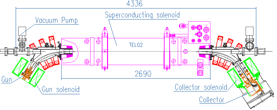
Applications of electron lenses often rely on the axial symmetry of the electrons’ current distribution. For instance, in a hollow electron beam scraper, the halo of the circulating beam is affected by the electromagnetic fields generated by the electrons Stancari:PRL:2011 . The beam core is unaffected only if the distribution of the electron charge is axially symmetric. One cause of asymmetry is the space-charge evolution of the electron beam as it propagates through the electron lens. In this note, we consider another effect: the bends that are usually used to inject and extract the electron beam from the interaction region (Figure 1). Although small, these asymmetries may have detectable effects on core lifetimes and emittances because of their nonlinear nature, especially when the current of the electron pulse is changed turn by turn to enhance the halo removal effect by resonant excitation of selected particles.
II Generation of the electron macroparticles
In this note, we focus on the configuration of hollow electron lenses for the LHC. The parameters of the proton beam are used to calculate beam sizes in the interaction region. Typical values are reported in Table 1. We assume a round proton beam with an rms beam size .
| Kinetic energy | Emittance (rms norm.) | Lattice function amplitude | Size (rms) | Divergence (rms) |
| [TeV] | [m] | [m] | [m] | [rad] |
The hollow electron beam is represented by a cylindrical bent pipe with a curvature radius , inner radius , and outer radius . The ratio between the outer and the inner radius is chosen to reproduce the dimensions of the cathode in the existing 1-inch hollow electron gun that was built as LHC prototype Li:TM:2012 ; Moens:Thesis:2013 : . The bent tube of electrons spans a bend angle of . A total of electron macroparticles is used to reproduce the static charge density distribution of a -A, -keV electron beam.
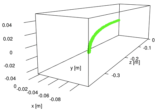
A subsample of the distribution of macroparticles is shown in Figure 2. The -axis is chosen along the direction of the circulating proton beam. The -axis points horizontally outward. The upward direction is represented by the -axis. The origin of the coordinate system coincides with the point where the axis of the bent electron beam intersects the axis of the circulating beam.
III Calculation of electrostatic fields
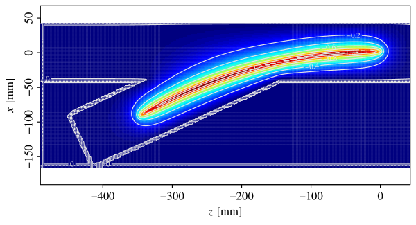

A multigrid Poisson solver within the Warp particle-in-cell code Vay:CSD:2012 is used to calculate the electrostatic fields. The Dirichlet boundary conditions are defined by a long cylindrical main beam pipe and by a cylindrical injection beam pipe stub, joining the main pipe at an angle (Figure 3). This arrangement is a simplified version of the injection scheme in the Tevatron electron lenses (Figure 1). Both pipes have an inner radius . The injection pipe is centered on the midpoint along the electron beam arc between the starting edge of the electron beam and the intersection point between the curved electron beam axis and the main pipe. The axis of the injection pipe is tangent to the electron beam axis at .
Space is subdivided into 2 discrete grids, a coarse one and a fine one. The coarse mesh has a spacing of and covers the whole simulated space, which extends at least 1 beam pipe radius beyond the charge distribution of the system. The fine mesh is constructed around the hypothetical central trajectory of the circulating proton beam. Its spacing is , or a fraction of . It extends longitudinally for the whole length of the simulated space. The coverage of the fine mesh is designed to obtain kick maps for both the core and the halo of the proton beam. We therefore define a region of interest: and , with . The fine mesh extends beyond the region of interest to smoothly connect with the coarse mesh.
Numerical simulations are run on Linux machines. A full calculation takes a few minutes on a single processor core. For the coarse mesh, all the relevant data is written to file: mesh coordinates, charge density, electrostatic potential, electric field components. For the fine mesh, only the integrated fields are saved (as described below). Data analysis, scripting, and report generation are done with the multi-platform, open-source statistical software R R:2013 .
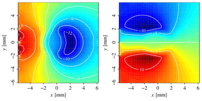
Figure 3 shows the electrostatic potential on the -plane of the bend. A section of the conductors is marked by the 0-V equipotential lines and by the grid points in light gray. The potential near the center of the electron beam is .
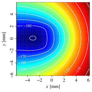
The electrostatic potential and the components of the electric field on the -axis (axis of the proton beam) of the coarse mesh are shown in Figure 4. As most of the charge lies on the side of the -plane, the -component of the electric field is negative. Because of symmetry, the vertical component should vanish. Its small fluctuations show the effect of the discrete distribution of charge. As expected, the -component of the electric field is positive for large negative , whereas it becomes negative after the protons cross the negative charge distribution.
IV Calculation of the transverse proton kicks
The electrostatic fields are integrated over straight paths to estimate the kicks on the circulating proton beam. Only transverse kicks are considered, as the longitudinal kicks of two symmetric bends cancel out for high-energy protons. The transverse kicks due to two bends, on the other hand, have the same sign and will add up. The typical angles of the proton trajectories are of the order of (Table 1), where and are Courant-Snyder lattice parameters. The resulting position variations of the protons over the length of the bend are therefore neglected.
From Newton’s second law, and neglecting magnetic effects, the transverse kick is related to the impulse of the electrostatic force :
| (2) | |||||
| (3) |
where , , , , , are the charge, velocity, relativistic factors, rest energy, and magnetic rigidity of the circulating beam, and is time. The integrated electric fields (loosely referred to as ‘kicks’) are defined as follows:
| (4) | |||||
| (5) |
and can be applied to particles of different magnetic rigidities. The results of the calculation are shown in Figure 6. Protons on axis experience a negative horizontal integrated field of , whereas the vertical kick vanishes. For 7-TeV protons, for instance, an integrated field of 10 kV generates an angular deviation of 1.4 nrad.
For tracking simulations, one could interpolate the kick maps of Figure 6 in 2 dimensions for each particle. Alternatively, for better accuracy and to speed up calculations, we look for an analytical symplectic parameterization of the functions and .
V Parameterization of the transverse kicks
The integrated potential is parameterized in terms of the tensor product of Chebyshev polynomials of the first kind up to order Press:NR:2007 :
| (6) | |||||
where are dimensional coefficients (in units of , for instance) and are Chebyshev polynomials of order in the variable :
| (7) | |||||
This parameterization is chosen because, in the interval , Chebyshev polynomials are orthogonal, making the coefficients independent of each other, and bounded, , making the coefficients of the same order of magnitude. (Because of the nonzero electron charge density on the proton trajectory, the electric potential does not satisfy Laplace’s equation and it cannot be derived from a complex harmonic potential decomposable as a superposition of multipoles.) The coordinates and are expressed in units of an arbitrary length scale ( for our region of interest), to ensure that the argument of the polynomials is contained within the unit interval. Because of the symmetry of the charge distribution, the potential should be an even function of and only contain even powers of the vertical coordinate. We therefore require
| (8) |
for any order of the polynomials in .
The kicks are obtained by derivation of the integrated potential:
| (9) | |||||
The derivatives of the Chebyshev polynomials can be calculated recursively as follows:
| (10) |
or from their trigonometric representation:
| (11) |
The cross derivatives of the kicks are
| (12) |
This ensures that the component of the curl of the integrated electric field is zero. This is a necessary and sufficient condition for the Jacobian matrix of initial and final transverse coordinates and momenta
| (13) |
to be symplectic:
| (14) |
because at any order of approximation.
In the region of interest, we have calculated points, each represented by the coordinates and fields , with . The polynomial model is applied simultaneously (i.e., with the same coefficients) to the integrated potential and to the kicks. Fitting only the integrated potential would introduce spurious effects in its derivatives as the order increases, whereas a fit to only the kicks cannot determine . The relative weights of and are set according to their ranges in the region of interest:
| (15) | |||||
The model is linear in the parameters, and the least-squares coefficients of this overdetermined system can be calculated by matrix inversion using singular-value decomposition (SVD) of the Vandermonde matrices of powers Press:NR:2007 :
| (16) |
Explicitly, we have
| (17) |
where the factors and are defined according to Eqs. 6, 9, and 15:
| (18) | |||||
Once the coefficients are found, the fitted values and the residuals are calculated as follows:
| (19) | |||||
| (20) |
An estimate of the random uncertainties on the coefficients is also provided by this procedure.

| E | E | E | E | E | E | E | E | E | ||
| E | E | E | E | E | E | E | E | 0 | ||
| E | E | E | E | E | E | E | 0 | |||
| E | E | E | E | E | E | E | E | 0 | 0 | |
| E | E | E | E | E | E | E | E | 0 | 0 | |
| E | E | E | E | E | E | E | 0 | 0 | 0 | |
| E | E | E | E | E | E | E | 0 | 0 | 0 | |
| E | E | E | E | E | E | 0 | 0 | 0 | 0 | |
| E | E | E | E | E | E | 0 | 0 | 0 | 0 | |
| E | E | E | E | E | 0 | 0 | 0 | 0 | 0 | |
| E | E | E | E | E | 0 | 0 | 0 | 0 | 0 | |
| E | E | E | E | 0 | 0 | 0 | 0 | 0 | 0 | |
| E | E | E | E | 0 | 0 | 0 | 0 | 0 | 0 | |
| E | E | E | 0 | 0 | 0 | 0 | 0 | 0 | 0 | |
| E | E | E | 0 | 0 | 0 | 0 | 0 | 0 | 0 | |
| E | E | 0 | 0 | 0 | 0 | 0 | 0 | 0 | 0 | |
| E | E | 0 | 0 | 0 | 0 | 0 | 0 | 0 | 0 | |
| E | 0 | 0 | 0 | 0 | 0 | 0 | 0 | 0 | 0 | |
| E | 0 | 0 | 0 | 0 | 0 | 0 | 0 | 0 | 0 |
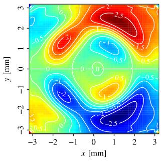
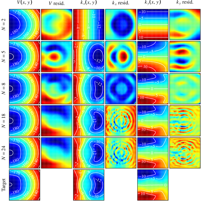
Figure 7 shows how the goodness of fit of the model (Eqs. 6, 8, and 9) varies as a function of the maximum order of the power series. The reconstructed integrated potential and the distribution of residuals as the order of the approximating polynomial increases are shown in Figure 8. At order (our chosen approximation), the standard deviation of the residuals of the integrated voltage is (compared to a total range of ). For the horizontal and vertical kicks, the standard deviations of residuals are and , respectively (over a total range of ). Inspection of the voltage residuals (Figure 8), shows a systematic effect roughly proportional to the vertical derivative of the integrated potential, suggesting that the potential is not exactly symmetric with respect to , but rather shifted by an amount of the order of the spacing of the fine mesh. This explains why the residuals do not decrease indefinitely with the order of the polynomial interpolation (Figure 7). This numerical artifact is negligible for our purposes.
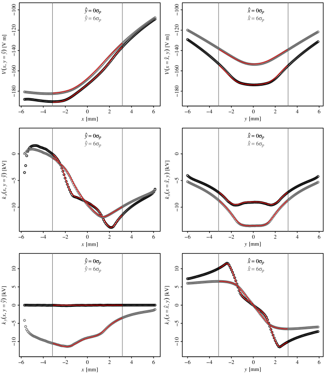
The one-dimensional dependence of the calculated and fitted functions , , and for a few sample cases is shown in Figure 9. The coefficients of the order polynomials and their statistical uncertainties are reported in Tables 2 and 3. The interpolated cross derivatives (Eq. 12) are shown in Figure 10.
VI Dependence of the results on the geometry of the system
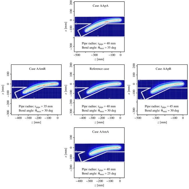
To study the sensitivity of the results to the geometry of the system, cases with different beam pipe radii and injection angles were simulated. The chosen beam pipe radii were , (reference case), and . These are the inner radii of both the main pipe and the injection pipe. The chosen bend angles were , (reference case), and . These are the angles spanned by the electron beam. Figure 11 shows the electrostatic potential on the bend plane () for each of these 5 cases.
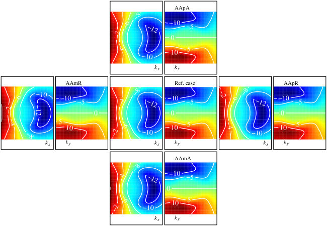
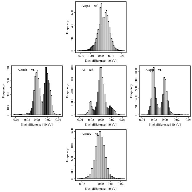
The calculated kick maps are compared in Figure 12. They look qualitatively very similar. A quantitative comparison is presented in Figure 13. Because the grid points are not exactly the same in each case, we randomly select 4096 points in the region of interest ( and ) and calculate the average kicks in their neighborhood for each case. The neighborhood is defined as 2 times the spacing of the fine grid. The histograms of the differences between the average kicks, divided by the arbitrary kick scale , are shown in Figure 13. The changes in geometry considered in this study amount to a change in the kicks limited to about 2.3% (or 0.23 kV).
VII Conclusions
The electrostatic fields generated by the bends in an electron lens were calculated. The corresponding symplectic kick maps were provided as coefficients of truncated power series of orthogonal polynomials for evaluation with analytical formulas. The goal is to asses some of the effects of electron-lens asymmetries on the circulating beam in the case of the proposed proton halo scraper for the LHC. The same technique can be applied to electron lenses with different current-density profiles (Gaussian, flat, etc.) to study perturbations in nonlinear integrable optics for the IOTA ring at Fermilab.
The present work may be further extended by taking into account the space-charge evolution of the electron beam, the magnetic fields, and longitudinal proton dynamics.
References
- (1) G. Stancari et al., in Proceedings of the 2013 North American Particle Accelerator Conference (NAPAC13), Pasadena, California, 29 September – 4 October 2013, p. 413, FERMILAB-CONF-13-355-APC.
- (2) G. Stancari et al., “Conceptual design of hollow electron lenses for beam halo control in the Large Hadron Collider,” FERMILAB-TM-2572-APC (2014).
- (3) S. Nagaitsev et al., in Proceedings of the 2012 International Particle Accelerator Conference (IPAC12), New Orleans, LA, USA, May 2012, p. 16, FERMILAB-CONF-12-247-AD.
- (4) A. Valishev et al., in Proceedings of the 2012 International Particle Accelerator Conference (IPAC12), New Orleans, LA, USA, May 2012, p. 1371, FERMILAB-CONF-12-209-AD-APC.
- (5) G. Stancari et al., Phys. Rev. Lett. 107, 084802 (2011).
- (6) S. Li and G. Stancari, FERMILAB-TM-2542-APC (August 2012).
- (7) V. Moens, Masters Thesis, École Polytechnique Fédérale de Lausanne (EPFL), Switzerland, FERMILAB-MASTERS-2013-02 and CERN-THESIS-2013-126 (August 2013).
- (8) J.-L. Vay, D. P. Grote, R. H. Cohen, and A. Friedman, Comput. Sci. Disc. 5, 014019 (2012).
- (9) R Core Team, “R: A language and environment for statistical computing,” R Foundation for Statistical Computing, Vienna, Austria. ISBN 3-900051-07-0, http://www.R-project.org.
- (10) W. H. Press, S. A. Teukolsky, W. T. Vetterling, and B. P. Flannery, Numerical Recipes: The Art of Scientific Computing (Cambridge University Press, 3rd ed., 2007)