On Modeling and Measuring the Temperature of the $z\sim 5$ IGM

Abstract

The temperature of the low-density intergalactic medium (IGM) at high redshift is sensitive to the timing and nature of hydrogen and HeII reionization, and can be measured from Lyman-alpha (Ly-$\alpha$) forest absorption spectra. Since the memory of intergalactic gas to heating during reionization gradually fades, measurements as close as possible to reionization are desirable. In addition, measuring the IGM temperature at sufficiently high redshifts should help to isolate the effects of hydrogen reionization since HeII reionization starts later, at lower redshift. Motivated by this, we model the IGM temperature at $z\gtrsim 5$ using semi-numeric models of patchy reionization. We construct mock Ly-$\alpha$ forest spectra from these models and consider their observable implications. We find that the small-scale structure in the Ly-$\alpha$ forest is sensitive to the temperature of the IGM even at redshifts where the average absorption in the forest is as high as $90\%$. We forecast the accuracy at which the $z\gtrsim 5$ IGM temperature can be measured using existing samples of high resolution quasar spectra, and find that interesting constraints are possible. For example, an early reionization model in which reionization ends at $z\sim 10$ should be distinguishable – at high statistical significance – from a lower redshift model where reionization completes at $z\sim 6$. We discuss improvements to our modeling that may be required to robustly interpret future measurements.

1. Introduction

The temperature of the low density intergalactic medium (IGM) after reionization retains information about when and how the gas was heated during the Epoch of Reionization (EoR) (e.g. Miralda-Escudé & Rees 1994; Hui & Gnedin 1997; Theuns et al. 2002a; Hui & Haiman 2003). The temperature of the IGM in turn impacts the statistical properties of the Ly-$\alpha$ forest towards background quasars and so the absorption in the forest provides “fossil” evidence regarding the timing and nature of reionization. Scrutinized carefully, this fossil may therefore improve our understanding of reionization. For example, the IGM will likely be cooler at $z\sim 5$ if most of the IGM volume reionized at relatively high redshift, near e.g. $z\sim 10$, than if reionization happened later, near say $z\sim 6$. If reionization occurs early, the gas has longer to cool and reaches a lower temperature than if it happens late, at least provided the gas is heated to a fixed temperature at reionization. In addition, the IGM temperature should be inhomogeneous, partly as a result of spatial variations in the timing of reionization across the universe (Trac et al., 2008; Cen et al., 2009; Furlanetto & Oh, 2009). Careful measurements of the IGM temperature after reionization should hence constrain the average reionization history of the universe, and may potentially reveal spatial variations around the average history as well.

Two separate phases of reionization are likely relevant for understanding the thermal history of the IGM: an early period of hydrogen reionization during which hydrogen is ionized, and helium is singly ionized by star-forming galaxies, and a later period in which helium is doubly-ionized by quasars, i.e. HeII reionization. Hydrogen reionization completed sometime before $z\sim 6$ or so (e.g. Fan et al. 2006, although it might conceivably end as late as $z\sim 5$ – see McGreer et al. 2011; Mesinger 2009; Lidz et al. 2007) , while mounting evidence suggests HeII reionization finished by $z\gtrsim 2.5-3$ (see e.g. Worseck et al. 2011; Syphers et al. 2011 and references therein). Many of the existing IGM temperature measurements focus on redshifts of $z\sim 2-4$ (Schaye et al., 2000; Ricotti et al., 2000; McDonald et al., 2001; Zaldarriaga et al., 2001; Theuns et al., 2002b; Lidz et al., 2010); in this case the temperature is likely strongly influenced by HeII reionization (e.g. McQuinn et al. 2009) and so these measurements mostly constrain helium reionization rather than hydrogen reionization.

In order to best constrain hydrogen reionization using the thermal history of the IGM, temperature measurements at higher redshift ($z\gtrsim 5$) are required. Indeed, recent work has started to probe the temperature at these early times. In particular, the recent study by Becker et al. (2012) includes a measurement at $z=4.8$; Bolton et al. (2011) and Raskutti et al. (2012) determine the $z\sim 6$ temperature in the special “proximity zone” region of the Ly-$\alpha$ forest close to the quasar itself; and the analysis in Viel et al. (2013) starts to bound the $z\gtrsim 5$ IGM temperature, although these authors focus on placing limits on warm dark matter models.

The temperature at these higher redshifts is unlikely to be significantly impacted by HeII reionization. In addition, the “memory” of intergalactic gas to heating during the EoR gradually fades and so measurements as close as possible to the EoR should, in principle, be most constraining. It is not, however, obvious that the IGM temperature can be measured accurately enough from the $z\gtrsim 5$ Ly-$\alpha$ forest to exploit the sensitivity of the high redshift temperature to the properties of reionization. In particular, the forest is highly absorbed by $z\sim 5$ with $z\gtrsim 6$ spectra showing essentially complete Gunn-Peterson (Gunn & Peterson, 1965) absorption troughs (Becker et al., 2001; Fan et al., 2006). An interesting question is then: what is the highest redshift at which it is feasible to measure the IGM temperature from the Ly-$\alpha$ forest?

Towards this end, the goal of this paper is to both model the thermal state of the $z\sim 5$ IGM, incorporating inhomogeneities in the hydrogen reionization process, and to quantify the prospects for actually measuring the IGM temperature using $z\gtrsim 5$ Ly-$\alpha$ forest absorption spectra. The outline of this paper is as follows. In §2, we describe the numerical simulations used in our analysis. In §3, we present plausible example models for the reionization history of the universe and describe our approach for modeling inhomogeneous reionization. We adopt a semi-analytic approach for modeling the resulting thermal history of the IGM, as described in §4. In this section, we also quantify the statistical properties of the temperature field in several simulated reionization models. Finally, in §5 we discuss how to measure the temperature from the $z\sim 5$ Ly-$\alpha$ forest, and forecast how well it may be measured with existing data. Our main conclusions are described in §6.

This work partly overlaps with previous work which also recognized the importance of, and modeled, temperature inhomogeneities in the $z\sim 5$ IGM and considered some of the observable implications (Trac et al., 2008; Cen et al., 2009; Furlanetto & Oh, 2009). One key difference with this earlier work is that we consider a more direct approach for measuring the temperature of the $z\sim 5$ IGM from the Ly-$\alpha$ forest. Our modeling of the thermal state of the IGM is closely related to that in Furlanetto & Oh (2009), except that we implement a similar general approach using numerical simulations, which allow us to construct mock Ly-$\alpha$ forest spectra and to measure the detailed statistical properties of these spectra. The works of (Trac et al., 2008; Cen et al., 2009) use radiative transfer simulations to model hydrogen reionization and the thermal history of the IGM and so these authors track some of the underlying physics in more detail than we do here. However, our approach here is faster, simpler, and more flexible, while we believe that it nevertheless captures many of the important processes involved.

2. Simulations

Our analysis makes use of two different types of numerical simulations. First, we use the “semi-numeric” scheme of Zahn et al. (2006) to model reionization; this algorithm is performed on top of the dark matter simulation of McQuinn et al. (2007a). The McQuinn et al. (2007a) simulation tracks $1024^{3}$ dark matter particles in a simulation volume with a co-moving sidelength of $130$ Mpc/$h$. Using the semi-numeric technique allows us to capture the impact of inhomogeneities in the reionization process, while providing the flexibility to explore a range of possible reionization models. In these models, we assume that the gas distribution closely traces the simulated dark matter distribution. We discuss the impact of this approximation when relevant. As we will describe, we map between the redshift of reionization of each gas element and its temperature at high redshift using the technique of Hui & Gnedin (1997); this mapping depends on the density of each gas element. We then produce mock Ly-$\alpha$ forest spectra, according to the usual “fluctuating Gunn-Peterson approximation” (e.g. Miralda-Escude et al. 1996; Croft et al. 2002) although here we additionally account for the temperature variations from inhomogeneous reionization.

We also make use of one of the smoothed particle hydrodynamic (SPH) simulations from Lidz et al. (2010). These simulations were run using the code Gadget-2 (Springel, 2005). This simulation tracks $2\times 1024^{3}$ particles (with equal numbers of dark matter and baryonic particles) in a $50$ Mpc/$h$ simulation box. In these calculations, we ignore the inhomogeneity of the reionization process. We use these simulations to more faithfully capture the gas distribution (for gas elements that reionize at a given time). In constructing mock Ly-$\alpha$ forest spectra from these simulations, we first modify the simulated gas temperatures, according to various prescriptions, in order to test how sensitive the statistical properties of the absorption are to the gas temperature.

3. Reionization Histories

In an effort to explore how the thermal state of the post-reionization IGM depends on the reionization history of the universe, we consider several example reionization histories. Our aim is to consider models that result in a wide range of possible thermal histories, while broadly maintaining consistency with current observational constraints on reionization.

For simplicity, we assume (as is common) that early galaxy populations produce ionizing photons at a rate that is directly proportional to the rate at which matter collapses into halos above some minimum mass. The minimum mass describes the host halo mass above which galaxies form readily; here we adopt $M_{\rm min}=10^{9}M_{\odot}$. We compute the collapse fraction from the Sheth-Tormen halo mass function (Sheth et al., 2001). With these assumptions, the volume averaged ionization fraction ($\langle x_{i}\rangle$) obeys the following differential equation (Shapiro & Giroux, 1987; Madau et al., 1999):

$$\frac{d\langle x_{i}\rangle}{dt}=\zeta\frac{df_{\rm coll}}{dt}-\frac{\langle x_{i}\rangle}{\bar{t}_{\rm rec}}.$$ (1)

The first term on the right hand side of the equation describes the rate at which neutral atoms are ionized, while the second term on the right hand side accounts for ionized atoms that recombine. The recombination time ($\bar{t}_{\rm rec}$) depends on the clumpiness of the IGM, parametrized by a “clumping factor”, $C=\langle n_{e}^{2}\rangle/\langle n_{e}\rangle^{2}$, and the temperature of the IGM. In solving this equation – and for this purpose only – we assume an isothermal IGM. We approximate the clumping factor and the temperature as independent of redshift. Adopting the case-B recombination rate in solving this equation, a temperature of $T_{0}=2\times 10^{4}$ K, and $C=3$ (see e.g. Pawlik et al. 2008; McQuinn et al. 2011b for a discussion regarding plausible values of the clumping factor) gives

$$\bar{t}_{\rm rec}=0.93{\rm Gyr}\left[\frac{3}{C}\right]\left[\frac{1+z}{7}\right]^{-3}\left[\frac{T_{0}}{2\times 10^{4}K}\right]^{0.7}.$$ (2)

Solving the differential equation, Eq. 1, suffices to compute the average ionization fraction as a function of redshift, given the minimum mass and efficiency, $\zeta$, of the ionizing sources.

In order to model reionization inhomogeneities, we use the “semi-numeric” scheme of Zahn et al. (2006), which is based on the excursion set model of reionization developed in Furlanetto et al. (2004). This scheme captures the tendency for halos – and hence galaxies – to form first in regions that are overdense on large scales, and to reionize before more typical locations in the universe. In the simplest version of the semi-numeric scheme, recombinations are considered only in an average sense and are treated as simply reducing the overall efficiency at which atoms are ionized. Let us denote the resulting efficiency factor as $\tilde{\zeta}(z)$ to distinguish it from the above ionizing efficiency factor $\zeta$. As we explain subsequently, we allow this efficiency factor to be redshift dependent. We can then consider the condition that a region of co-moving size $R$ is ionized. In the initial conditions, the mass enclosed within this co-moving region is $M=4\pi R^{3}\langle\rho_{M}\rangle/3$, with $\langle\rho_{M}\rangle$ denoting the average matter density per co-moving volume. The condition for this region to be ionized is then:

$$\tilde{\zeta}(z)f_{\rm coll}(>M_{\rm min}|\delta_{M},M)\geq 1.$$ (3)

In this equation $f_{\rm coll}(>M_{\rm min}|\delta_{M},M)$ is the conditional collapse fraction, i.e., the fraction of mass in halos above the minimum mass ($M_{\rm min}$) in a region of linear overdensity $\delta_{M}$. Here $\delta_{M}$ denotes the overdensity when the linear density field is smoothed on mass scale $M$.

In order to tabulate a reionization redshift for many grid cells across the volume of our simulation, we smooth the density field – linearly evolved from the initial conditions – on a range of mass scales, starting from large scales and stepping downward until we reach the scale of each simulation cell. For each simulation cell, and across all smoothing scales considered, we record the highest redshift at which the ionization barrier (Eq. 3) is crossed. This highest crossing redshift is considered to be the reionization redshift, $z_{r}$, for the cell in question. We tabulate reionization redshifts for each of $512^{3}$ grid cells. This provides us with a reasonable model for the expected spatial variations in the redshift of reionization – and the coherence scale of these inhomogeneities – across the simulation volume.

Note that here we approximate the excursion set model as determining the redshift at which each volume element is reionized, although in reality mass elements move from their initial positions, and overdense regions expand less rapidly than typical locations. This approximation is commonly made, and is reasonable given the large size of the ionized regions (Furlanetto et al., 2004) and the correspondingly large coherence scale of the spatial variations in the reionization redshift.

Another ingredient we use from the McQuinn et al. (2007a) simulation is the evolved non-linear dark matter density field, interpolated onto the same grid (using CIC interpolation) as the reionization redshifts. For our calculations with this simulation, we generally assume that the gas distribution follows the simulated, gridded dark matter distribution. Note that the smoothing introduced by gridding the dark matter particles is comparable to the Jeans smoothing scale: the co-moving Jeans wavenumber for isothermal gas at $10^{4}$ K, is $k_{J}=13h$ Mpc^-1 at $z=5$ which is comparable to the Nyquist wavenumber of the grid, $k_{\rm Nyq}=12h$ Mpc^-1. More relevant, however, is the “filtering scale” – essentially a time-averaged Jeans scale – and this should be smaller than the Jeans scale by around a factor of a few (Gnedin & Hui, 1998). In any case a single global smoothing only roughly approximates the full effect of Jeans smoothing. We will return to discuss this further in §5 and §5.3. In particular, in order to approximately capture the impact of small scale structure and thermal broadening in our mock quasar spectra, we will add small-scale structure using a lognormal model. Although using the gridded dark matter density field to represent the gas distribution is inadequate for making detailed mock spectra, it suffices for our model of the temperature distribution of the low density gas.

Returning to further consider the semi-numeric modeling, an important caveat is that this algorithm does not return precisely the expected volume-averaged ionization fraction (see the Appendix of Zahn et al. 2006 for a discussion). Here we simply tune $\tilde{\zeta}(z)$ to produce the desired redshift evolution of the ionization fraction. Although this procedure is not ideal, small adjustments to the ionizing efficiency factor have little impact on the size of the ionized regions at a given volume-averaged ionization fraction, $\langle x_{i}\rangle$, and so this approach is adequate for our present purposes.

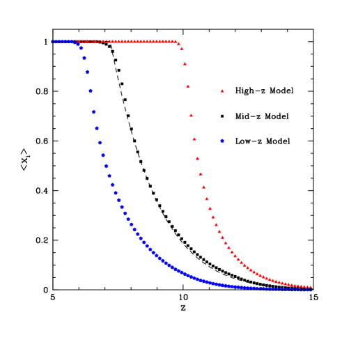
Figure 1.— Example reionization histories. The red triangles show the simulated volume-average ionization fraction in our semi-numeric High-z reionization model, the black squares are for the Mid-z reionization scenario, and the blue pentagons are for a low redshift (Low-z) reionization model. The black dashed line shows the reionization history computed by solving Eq. 1 with $\zeta=46$, $M_{\rm min}=10^{9}M_{\odot}$ and $C=3$. The semi-numeric efficiency parameters $\tilde{\zeta}(z)$ in the Mid-z case have been tuned to match this model.

The redshift evolution of the volume-averaged ionization fractions are shown in Fig. 1 for three example models. The symbols show the average ionized fraction from the simulation cube at different redshifts. We call the three examples in the figure the “Low-z” model, the “Mid-z” model, and the “High-z” model. The Mid-z model adopts a redshift dependent efficiency factor of the form $\tilde{\zeta}(z)=35(1+z/13)^{1.75}$ for $z\leq 12$ and $\tilde{\zeta}=35$ for $z>12$. For comparison, the black dashed line shows the solution to Eq. 1 for a model with $\zeta=46$, $C=3$, and $M_{\rm min}=10^{9}M_{\odot}$. Hence the semi-numeric scheme in the Mid-z model has been tuned to return the ionized fraction expected from Eq. 1 for a plausible model. The Low-z and High-z models are similar to the Mid-z model, except that the efficiency factor in the semi-numeric models has been adjusted to $\tilde{\zeta}(z)=12(1+z/11)^{0.60}$ at $z\leq 10$ and to $\tilde{\zeta}(z)=12$ at $z>10$ for the Low-z model and to a constant efficiency factor $\tilde{\zeta}(z)=70$ for the High-z model. (Although these alternative models were not themselves explicitly tuned to match particular solutions to Eq. 1, the general behavior is similar to in the Mid-z model except that reionization happens a little later/earlier in the Low-z/High-z model and so these models also appear reasonable).

It is also useful to quantify the timing and duration of reionization, as well as the optical depth to Thomson scattering ($\tau_{e}$), in each model. Defining the “completion” of reionization as the redshift where the volume averaged ionization fraction first reaches $\langle x_{i}\rangle=1$, the High-z model completes at $z=9.6$, the Mid-z model at $z=6.7$, and the Low-z model at $z=5.8$. As one measure of the “duration” of reionization, we consider the redshift spread over which $\langle x_{i}\rangle$ evolves from $\langle x_{i}\rangle=0.1$ to $\langle x_{i}\rangle=1$. This duration is $\Delta z=2.7,4.3,3.5$ for the High-z, Mid-z, and Low-z models. Note that the duration is the longest in the Mid-z model because the ionizing efficiency factor $\tilde{\zeta}(z)$ has the strongest redshift dependence in this case. The electron scattering optical depths are $\tau_{e}=0.088,0.066,0.052$ for the High-z, Mid-z, and Low-z reionization models respectively. These values assume that the fraction of helium that is singly ionized is identical to the fraction of hydrogen that is ionized, and ignore the slight boost expected from the free electrons produced after HeII reionization, which we do not track in this work.

The present constraint on $\tau_{e}$ from Planck CMB temperature anisotropy data (Ade et al., 2013), combined with the E-mode polarization power spectrum at large angular scales from WMAP nine year data (Bennett et al., 2013), is $\tau_{e}=0.089^{+0.012}_{-0.014}$. Most of the constraining power here comes from the WMAP polarization data. Hence our High-z model produces a $\tau_{e}$ close to the presently preferred value, the Mid-z model is low by $1.6-\sigma$, while the Low-z model is too low by $2.6-\sigma$. Hence our lower redshift reionization models are already marginally disfavored, but they are still certainly worthy of further investigation. The Planck collaboration should soon announce new large-scale CMB polarization measurements; the improved frequency coverage of the Planck satellite should help guard against foreground contamination, and further test these models for $\tau_{e}$. Although the current $\tau_{e}$ constraints allow higher reionization redshift models than the three examples considered here, the $z\sim 5$ IGM temperature is insensitive to the reionization redshift if reionization happens above $z\gtrsim 10$ (§4, Hui & Haiman 2003). While viable, we need not consider such models explicitly here since in these cases the $z\sim 5$ temperature will be similar to that in our High-z model.

4. The Thermal State of the IGM

We now explore how the thermal state of the $z\sim 4-6$ IGM depends on the reionization history of the Universe, using the example histories of the previous section. In this section, we focus mostly on the Low-z and High-z models since they span a fairly wide range of possibilities for the IGM temperature at the redshifts of interest.

The key equation describing the thermal evolution of a gas element in the IGM is (e.g. Hui & Gnedin 1997):

$$\frac{dT}{dt}= -2HT+\frac{2T}{3(1+\delta)}\frac{d\delta}{dt}+\frac{T}{\mu}\frac{d\mu}{dt}$$

$$+\frac{2\mu m_{p}}{3\rho k_{B}}\left({\mathcal{H}}-\Lambda\right).$$ (4)

The first term on the right hand side accounts for adiabatic cooling owing to the overall expansion of the universe. The second term describes adiabatic heating/cooling from structure formation, i.e. from gas elements contracting/expanding. In the third and fourth terms, $\mu$ is the mean mass per free particle in the gas, in units of the proton mass. The third term accounts for the temperature change that occurs because the mean mass per particle may change with time. ${\mathcal{H}}$ describes the heating term, while $\Lambda$ is the cooling function of the gas. These terms describe the heat gain and loss per unit volume, per unit time, in the gas.

Let us first summarize the qualitative behavior of the solutions to Eq. 4, focusing on the low density intergalactic gas that fills most of the volume of the universe (see also Miralda-Escudé & Rees 1994; Hui & Gnedin 1997; Hui & Haiman 2003; Furlanetto & Oh 2009). During reionization, most gas elements are rapidly ionized and change their ionization fraction by order unity. The excess energy of the ionizing photons (above the ionization threshold) goes into the kinetic energy of the outgoing electrons, which quickly share their energy with the surrounding gas, and raise its temperature. The first thing to consider is hence the initial temperature reached at reionization. Provided the gas becomes highly ionized, its temperature boost during reionization depends only on the shape of the spectrum – and not the amplitude – of the radiation that ionized it.

In detail, we expect gas elements to be ionized by radiation with a range of spectral shapes. This should be the case both because the intrinsic ionizing spectrum will vary from galaxy to galaxy, and because the spectral shape may be hardened by intervening absorption, which will itself vary spatially depending on the column density of neutral gas between an ionizing source and an absorber. On the other hand, the ionized regions during hydrogen reionization likely grow under the collective influence of numerous (yet individually faint) dwarf galaxies (e.g. Robertson et al. 2013), and so some of these variations may average down, provided gas elements are ionized by a combination of several sources and the ionizing radiation arrives along various different pathways. In any case, modeling the precise temperature input during reionization and its spatial variations requires full radiative transfer simulations and is well beyond the scope of our approach here. We adopt this uniform temperature boost approximation throughout, and discuss plausible values for the input temperature subsequently. Note also that in this case the temperature boost during reionization is independent of density: extra heat is put into the overdense regions since more atoms are ionized in these regions, but the heat is shared across the larger number of particles in the overdense parcel.

After a gas element is reionized, it settles into ionization equilibrium and the UV radiation from the ionizing sources keeps the gas highly ionized (at least for the low density gas parcels that fill most of the volume of the IGM). In ionization equilibrium, each recombination is balanced by a photoionization and the ionizations in turn heat the gas; the average time between recombinations in the low density IGM is long, and so the heat input from photoionization is significantly reduced after a parcel becomes highly ionized during reionization. In addition, the spectral shape of the ionizing radiation incident on a typical gas element should soften – i.e., the average heat input per photoionization should drop – after reionization as the optical depth to ionizing photons decreases (Abel & Haehnelt, 1999).

The dominant cooling processes are adiabatic cooling from the expansion of low density gas parcels and Compton cooling off of the CMB. As a result of cooling, although gas elements that reionize at the same time start off with identical temperatures, irrespective of their density, parcels with differing densities will not stay at the same temperature. In particular, the low density elements expand and cool faster than typical regions, while overdense regions recombine faster and thus – in ionization equilibrium – gain more heat from photoionizations after reionization. In addition, sufficiently overdense regions will be heated by adiabatic contraction. Hui & Gnedin (1997) showed that this competition between adiabatic cooling/heating, Compton cooling, and photoionization heating, drives the intergalactic gas to generally land on a tight temperature-density relation of the form $T=T_{0}(1+\delta)^{\gamma-1}$. Both the temperature at mean density, $T_{0}$, and the slope of the temperature density relation, $\gamma$, depend on the reionization redshift; $T_{0}$ falls off and $\gamma$ becomes steeper as the gas cools after reionization, until the gas gradually loses memory of the heating during reionization. In the previous work of Hui & Gnedin (1997), however, all of the gas was assumed to reionize at the same redshift. Here we would like to generalize this to incorporate spatial variations in the redshift of reionization (see also Furlanetto & Oh 2009 and Hui & Haiman 2003).

4.1. Modeling the Thermal State

In general, to follow the thermal evolution in Eq. 4 we should combine this equation with equations specifying the evolution of the ionized fraction of each different particle species. However, for our present application a simpler approach should suffice. In particular, we start by assuming that each parcel is heated to a common temperature, $T_{r}$, at its reionization redshift, $z_{r}$. We then follow the subsequent thermal evolution after a gas element is ionized by assuming ionization equilibrium and that each element is highly ionized (as in Furlanetto & Oh 2009). More specifically, we assume that both HI and HeI are highly ionized, but that HeII is not yet ionized, i.e., that HeII reionization starts later than the high redshifts of interest for our study. We further assume the gas is composed of only hydrogen and helium, neglecting metal line cooling, and also molecular hydrogen cooling, which should be very good approximations for the low density IGM. In addition to adiabatic heating/cooling and Compton cooling, we track HI photoheating, HeI photoheating, and recombination cooling of HII/HeII using the rate expressions in the Appendix of Hui & Gnedin (1997). We ignore collisional ionizations, and HI/HeI/HeII line excitation cooling: neglecting these processes should be a good approximation for the low density and highly ionized gas that fills most of the IGM volume after reionization. Furthermore, we ignore other potential heating sources such as shock heating, galactic winds, blazar heating, etc..(see e.g. Hui & Haiman 2003; Chang et al. 2012 and references therein for a discussion). In the Appendix we also derive approximate solutions using linear perturbation theory (incorporating only HI photoheating, Compton cooling, and adiabatic cooling/heating), that are useful for fast and fairly accurate estimates (see also Hui & Gnedin 1997).

In principle we could calculate the adiabatic expansion/contraction term (second term in Eq. 4) directly from the McQuinn et al. (2007a) simulation, at least under the approximation that the gas distribution traces the simulated dark matter density field. Here we instead follow the approach of Hui & Gnedin (1997) and compute this term for tracer elements assuming their density evolution obeys the Zel’dovich approximation (Zel’dovich, 1970). As mentioned earlier, we do, however, extend this calculation to consider gas elements with a range of different reionization redshifts.

The basic premise here is that gas elements with identical reionization redshifts should land on a well-defined temperature-density relation (as supported by the tests in Hui & Gnedin 1997 and subsequent work); we can determine this relation by solving Eq. 4 for many sample gas parcels. Incorporating, however, the spread in reionization redshifts, and that the reionization redshift of each parcel may correlate with its density, a perfect temperature-density relation will not generally be a good description. In other words, we follow sample gas parcels to determine the mapping between the temperature-density relation at a given redshift and the reionization redshift and temperature, i.e., this is used to determine $T_{0}(z|z_{r},T_{r})$ and $\gamma(z|z_{r},T_{r})$. These mappings can then be applied to our reionization simulation to determine the temperature of any gas element, given its reionization redshift and overdensity. To determine $T_{0}(z|z_{r},T_{r})$ and $\gamma(z|z_{r},T_{r})$, we follow the thermal evolution for $20,000$ tracer elements for many different reionization redshifts, assuming their density evolves according to the Zel’dovich approximation, and fit separate power-laws for each $z,z_{r}$, and $T_{r}$.

In the Zel’dovich approximation, the density field evolves according to the equation:

$$1+\delta=\frac{1}{\rm{det}[\delta_{ij}+D(t)\psi_{ij}]},$$ (5)

with $\psi_{ij}$ denoting the initial deformation tensor, and $D(t)$ denoting the linear growth factor (normalized to unity today). The density evolution of a tracer element can then be specified by the eigenvalues of the local initial deformation tensor. As in Hui & Gnedin (1997) and Reisenegger & Miralda-Escude (1995), we can construct realizations of the density evolution in the Zel’dovich approximation by randomly drawing eigenvalues of $\psi_{ij}$ from the expected probability distribution (Doroshkevich, 1970). We do this following Hui et al. (2000); Bertschinger & Jain (1994).

In our fiducial model, we take the temperature at reionization to be $T_{r}=2\times 10^{4}$ K (see Furlanetto & Oh 2009; McQuinn 2012 for a discussion of this choice). In calculating the photoionization heating term after a gas parcel reionizes, we assume that the specific intensity of the ionizing radiation is a power-law in frequency close to the hydrogen photoionization threshold, $J(\nu)\propto\nu^{-\alpha}$ with $\alpha=1.5$. As mentioned previously, the heat input is insensitive to the amplitude of the ionizing radiation, provided the gas is highly ionized. This spectral shape is intended to be somewhat harder than expected for the intrinsic spectrum of the ionizing sources, since intervening absorption will harden this spectrum (Zuo & Phinney, 1993; Hui & Haiman, 2003; Furlanetto & Oh, 2009).

4.2. Simulated Temperature Field

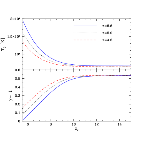
Figure 2.— Thermal state of gas elements with a given reionization redshift, as a function of that redshift. In each case, the gas elements are heated to a temperature of $T_{r}=2\times 10^{4}$ K during reionization, and the residual photo-heating after reionization is computed assuming that the (hardened) spectral index of the ionizing sources is $\alpha=1.5$ near the HI photoionization edge. Top panel: The temperature at mean density ($T_{0}$) for gas elements at each of $z=4.5,5.0$ and $5.5$ as a function of their reionization redshift. Bottom panel: This is similar to the top panel, except it shows the slope of the temperature-density relation ($\gamma-1$) rather than $T_{0}$. Note that although we assume that gas elements with a given reionization redshift all land on a well defined temperature-density relation, this will not generally be a good description once we account for the spread in reionization redshift across the universe.

We now examine the properties of the simulated temperature field, modeled as described in the previous section. First, we consider the mapping between the temperature at mean density, $T_{0}$, and the slope of the temperature-density relation, $\gamma$, for gas at various redshifts, given the reionization redshift, $z_{r}$, of each gas element. This is shown, for our baseline set of assumptions, in Fig. 2 for each of $z=4.5,5.0,$ and $z=5.5$. The values of $T_{0}$ are close to the temperature at reionization ($T_{r}=2\times 10^{4}$ K) for gas elements that ionized at redshifts just above $z=5.5$, since these elements have had very little time to cool. On the other hand, gas parcels with higher $z_{r}$ have had longer to cool and are hence at lower temperatures. For instance, gas elements that reionized at $z_{r}=8$ have cooled down to $T_{0}=8,800$ K by $z=5.5$, more than a factor of two below the temperature at reionization. The temperatures of gas elements that reionize at sufficiently high redshift, however, become insensitive to the precise redshift of reionization. In particular, gas elements that reionize above $z_{r}\gtrsim 10$ are all at $T_{0}=6,700$ K at $z=5.5$, irrespective of $z_{r}$. This results mainly because Compton cooling is very efficient at high redshift ($z\gtrsim 10$), and effectively erases the memory of the photoheating during reionization (Hui & Gnedin, 1997). Indeed, this is the main reason that we don’t consider still higher redshift reionization models, although they would be allowed by the present $\tau_{e}$ constraints as discussed in §3 (but perhaps disfavored by other data sets, see e.g. Robertson et al. 2013; Kuhlen & Faucher-Giguere 2012 for recent summaries.): the thermal state of the IGM is insensitive to higher redshift reionization models.

The bottom panel is similar to the top panel except here we plot $\gamma-1$ versus $z_{r}$. Gas elements that reionize just above $z=5.5$ are close to isothermal, while elements that ionize at $z_{r}\gtrsim 10$ have a steeper slope, $\gamma=1.53$. The $T_{0}$ and $\gamma-1$ curves at $z=4.5$ and $z=5.0$ illustrate less sensitivity to $z_{r}$, since gas elements at these redshifts have had longer to cool down from their initial temperatures at reionization. Nevertheless, the models at these lower redshifts still certainly do show some dependence on $z_{r}$.

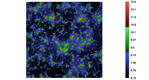
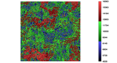
Figure 3.— Reionization redshifts and temperatures at $z=5.5$ in the low-z reionization model. Top panel: The reionization redshifts for a narrow slice ($0.25$ Mpc/$h$ thick) through the simulation. Each slice is $130$ Mpc/$h$ on a side. The red regions indicate locations with the highest reionization redshifts across the simulation slice, while the dark regions are the last to be reionized. Bottom panel: The temperature of the same slice as in the top panel. The red areas in this panel show the hottest locations in the slice, and correspond to the dark regions in the top panel that are reionized late. The dark blue regions in the temperature slice, on the other hand, are the coolest regions that reionized first. The color scales are chosen so that $99\%$ of simulation cells in the slice shown here have redshifts and temperatures falling between the minimum and maximum values on the color bar.

We then use the curves plotted in Fig. 2 as a mapping to predict the temperature of various grid cells in our simulation given their overdensities, $\delta$, and reionization redshifts, $z_{r}$. This procedure allows us to model the temperature field across the entire simulation volume at various redshifts.

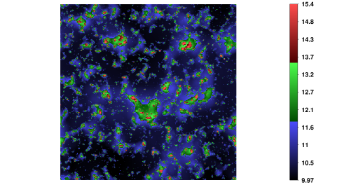
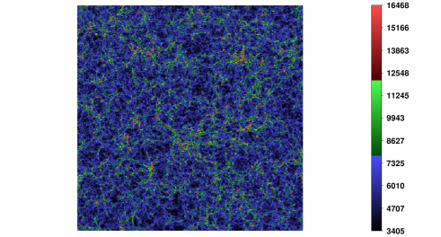
Figure 4.— Reionization redshifts and temperatures at $z=5.5$ in the high-z reionization model. Identical to Fig. 3, except this figure shows the contrasting High-z model. Note that the color scale in this case also encompasses $99\%$ of the reionization redshifts and temperatures in the simulation slice, but that these ranges are different than in the previous figure.

Figs. 3 and 4 show the result of applying the mapping (at $z=5.5$) to the simulated density field. Specifically, these figures show thin slices ($0.25$ Mpc/$h$ thick) through the simulation volume, with the top panel showing the reionization redshift and the bottom panel the corresponding temperature of cells in the simulation volume. In the Low-z model (Fig. 3), the temperature field has sizable spatial variations on large scales. As anticipated earlier, these result because of the spread in the timing of reionization across the universe. As one can infer from the slice, the regions that are at low-density (when the density field is smoothed on large-scales) – i.e., the “voids” in the density distribution – are the last to reionize. These regions are at the highest temperature shortly after reionization because they have had the least amount of time to cool (see also Trac et al. 2008; Furlanetto & Oh 2009).

In contrast, the temperature field in the High-z model (Fig. 4) has mostly lost memory of the heating during reionization and so the temperature variations are more subtle here. This is expected from Figs. 1 and 2: much of the gas in this model is reionized at $z_{r}\gtrsim 10$, and efficient Compton cooling mostly removes the memory of reionization in this case. The temperature variations that are apparent in the High-z model instead reflect the usual temperature-density relation, as the competition between cooling and heating after reionization drives overdense regions to larger temperatures. These temperature variations are primarily coherent on the Jeans/filtering scale and so, as evident from the simulation slices, these fluctuations are concentrated mostly on smaller scales than the ones induced by the spread in the timing of reionization.

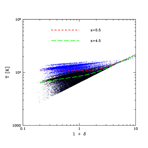
Figure 5.— Temperature density relations at $z=4.5$ and $z=5.5$ in the Low-z reionization model. The blue points show the temperature and density of gas elements from the simulation at $z=5.5$, while the black points are the same at $z=4.5$. The red short dashed line shows the median simulated temperature as a function of density at $z=5.5$. The green long dashed line is the same at $z=4.5$.

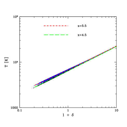
Figure 6.— Temperature density relations at $z=4.5$ and $z=5.5$ in the High-z reionization model. Identical to Fig. 5, except the results here are for the High-z reionization model.

A further, more quantitative description is provided by constructing scatter plots of the temperatures of many simulated gas elements as a function of their densities. This is shown in Figs. 5 and 6 for the Low-z and High-z reionization models, respectively. Broadly similar results may be found in earlier work by Trac et al. (2008) and Furlanetto & Oh (2009). The red short-dashed line in each figure shows the median gas temperature at $z=5.5$, while the green long-dashed line is the median temperature at $z=4.5$. Fig. 5 shows that the temperature of the $z=5.5$ IGM is generally rather high – and has a large amount of scatter at low densities – in the Low-z reionization model. By contrast, the temperature in the High-z reionization model (Fig. 6) is smaller – e.g., by 60% for the median temperature near the cosmic mean density – as is the scatter. In the Low-z model the median temperature is a fairly flat function of density for gas less dense than the cosmic mean.

Note that although the regions that have low density – when the density field is averaged on large scales – ionize last and are mostly hotter than denser regions (see Fig. 3), this does not fully “invert” the temperature-density relation. This is because the density field on the scale of the simulation grid (and at the Jeans scale) is only somewhat correlated with the larger scale density variations that determine the spread in the timing of reionization in our model. In any case, in agreement with previous work (Trac et al., 2008; Furlanetto & Oh, 2009), the usual temperature-density relation is a poor description of the thermal state of the IGM in the Low-z model at $z=5.5$. At slightly lower redshifts, $z=4.5$, the temperature has dropped somewhat and the scatter in the Low-z model has partially subsided, although it is still substantial. The median temperatures in the two reionization models are closer to each other by $z=4.5$, but they still differ by 30%.

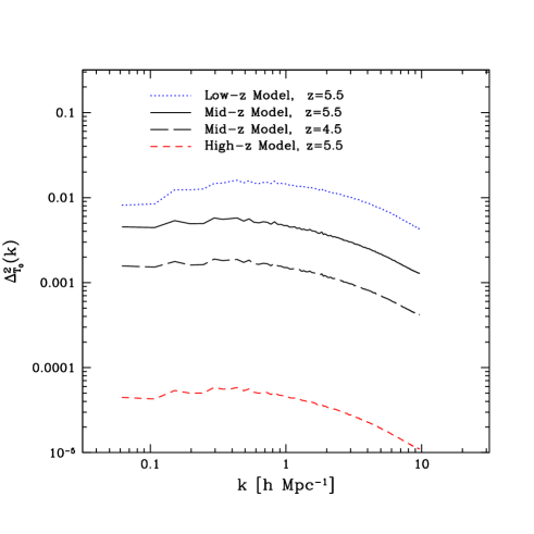
Figure 7.— Power spectrum of temperature fluctuations in various models. The curves show the power spectrum of $\delta_{T_{0}}({\mathchoice{{\hbox{\BFd x}}}{{\hbox{\BFt x}}}{{\hbox{\BFs x}}}{{\hbox{\BFss x}}}})=(T_{0}({\mathchoice{{\hbox{\BFd x}}}{{\hbox{\BFt x}}}{{\hbox{\BFs x}}}{{\hbox{\BFss x}}}})-\langle T_{0}\rangle)/\langle T_{0}\rangle$ from the simulated models. The blue dotted line, the black solid line, and the red short-dashed line are the power spectra at $z=5.5$ in the Low-z, Mid-z, and High-z models respectively. The black long-dashed line shows the $\delta_{T_{0}}$ power spectrum at $z=4.5$ in the Mid-z model to illustrate how the temperature fluctuations fade with time.

It is also useful to calculate the power spectrum of temperature fluctuations in each model. Since we are assigning a value of $T_{0}$ and $\gamma$ to each grid cell in the simulation volume, we can easily consider the power spectrum of $T_{0}$ rather than the power spectrum of the full temperature field. The advantage of considering the power spectrum of $T_{0}$ is that this power spectrum vanishes in the case of homogeneous reionization. In the case of homogeneous reionization, the temperature is a power-law in the gas density, and so the full temperature field still has (mostly small scale) fluctuations sourced directly by density inhomogeneities. Hence we consider here the power spectrum of $T_{0}({\mathchoice{{\hbox{\BFd x}}}{{\hbox{\BFt x}}}{{\hbox{\BFs x}}}{{\hbox{\BFss x}}}})$, or more precisely the power spectrum of $\delta_{T_{0}}({\mathchoice{{\hbox{\BFd x}}}{{\hbox{\BFt x}}}{{\hbox{\BFs x}}}{{\hbox{\BFss x}}}})=(T_{0}({\mathchoice{{\hbox{\BFd x}}}{{\hbox{\BFt x}}}{{\hbox{\BFs x}}}{{\hbox{\BFss x}}}})-\langle T_{0}\rangle)/\langle T_{0}\rangle$. Although the power spectrum of this field is not directly observable, it nevertheless helps to characterize the temperature fluctuations from reionization.

The power spectra in some of our models are shown in Fig. 7. Specifically, the curves show $\Delta^{2}_{T_{0}}=k^{3}P_{T_{0}}(k)/(2\pi^{2})$, the contribution to the variance of $\delta_{T_{0}}$ per natural logarithmic interval in $k$, i.e., per ${\rm dln}(k)$. In the Low-z model, the temperature fluctuations peak at a level of around $\sqrt{\Delta^{2}_{T_{0}}(k)}\approx 15\%$. We should keep in mind, however, that the scatter in the temperature at lower density is larger than at mean density (see Fig. 5). As a result, the power spectra of $T_{0}$ shown here hence do not fully capture the impact of inhomogeneous reionization, but they do nevertheless illustrate the spatial scale of the reionization induced inhomogeneities as well as their redshift and model dependence. The power spectra ($\Delta^{2}_{T_{0}}$) are evidently fairly flat functions of $k$. This is not surprising, since the power spectra of the fluctuations in the ionization field are also rather flat functions of $k$ during most of the EoR (e.g. McQuinn et al. 2007b). At the same redshift, the $\delta_{T_{0}}$ power spectrum in the Mid-z Model is $\approx 3$ times smaller in amplitude than in the Low-z model, while the amplitude of variations ($\Delta^{2}_{T_{0}}(k)$) in the High-z model are $\approx 300$ times smaller than in the Low-z model. As discussed previously, the small fluctuations in the High-z model result because Compton cooling is efficient at high redshift and this rapid cooling effectively erases the memory of heating at higher redshifts. Comparing the black solid and dashed lines illustrate how the fluctuations fade from $z=5.5$ to $z=4.5$ in the Mid-z model.

These models illustrate the dependence of the thermal history of the IGM on the timing of reionization; let us briefly summarize our main findings here. The IGM temperature for models in which a significant fraction of the IGM volume is reionized at relatively low redshift, near $z\sim 6$, is correspondingly larger than if most of the gas is reionized at higher redshift. In addition, the late reionization models produce sizable temperature inhomogeneities with fluctuations on scales as large as $\sim$ tens of co-moving Mpc.

4.3. Variations around Fiducial Parameters

Before we proceed to discuss the observable signatures of the IGM temperature models, it is interesting to consider how variations around our fiducial assumptions regarding the reionization temperature, $T_{r}$, and the shape of the ionizing spectrum after reionization might impact the resulting thermal state of the IGM. To investigate this, we consider models where the reionization temperature is $T_{r}=3\times 10^{4}$ K and $T_{r}=1\times 10^{4}$ K to contrast with our fiducial model in which $T_{r}=2\times 10^{4}$ K. The low $T_{r}$ model requires sources with extremely soft ionizing spectra, and is meant to represent a lower limit to the plausible reionization temperature, while the higher temperature $T_{r}=3\times 10^{4}$ K case is more reasonable (e.g. McQuinn 2012). In addition, for our fiducial reionization temperature we produce models with (post reionization) spectral shapes of $\alpha=0.5$ and $\alpha=2.5$ to compare with our baseline assumption of $\alpha=1.5$.

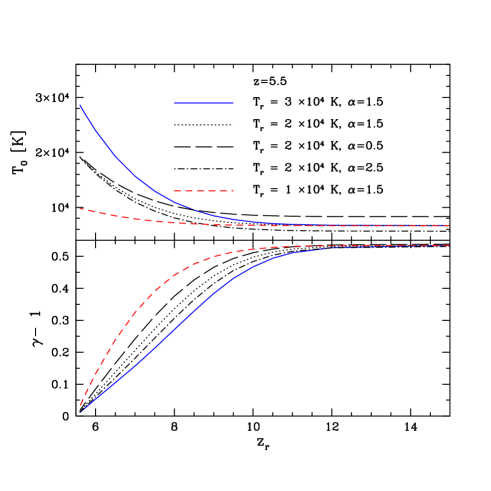
Figure 8.— Thermal state at $z=5.5$ for various reionization temperature and spectral shape models. This is similar to the $z=5.5$ curves in Fig. 2, except here we vary the reionization temperature, $T_{r}$, and the spectral shape, $\alpha$. Increasing $T_{r}$ leads to a higher $T_{0}$ and a flatter $\gamma$ for recently reionized gas parcels, while parcels that reionize at sufficiently high redshifts are insensitive to $T_{r}$. A harder ionizing spectrum after reionization (smaller $\alpha$) leads mostly to a slightly larger value of the asymptotic temperature achieved at high $z_{r}$. The harder spectrum also slightly hastens the transition of $\gamma$ to its asymptotic value.

First, we consider how our models for $T_{0}(z=5.5|z_{r})$ and $\gamma(z=5.5|z_{r})$ depend on the reionization temperature and spectral shape, i.e., we regenerate the models of Fig. 2 for different values of $T_{r}$ and $\alpha$. The results of these calculations are shown in Fig. 8. The first feature to note is that $T_{0}$ and $\gamma$ are independent of $z_{r}$ and $T_{r}$ in the limit of large reionization redshift: efficient cooling wipes out the memory of the early heating history. On the other hand, the $z=5.5$ temperature is naturally quite sensitive to the reionization temperature if reionization occurred relatively recently. One consequence of this is that the scatter in the $z\sim 5$ temperature will be larger in low redshift reionization models for cases with larger reionization temperatures: a high reionization temperature increases the temperature contrast between recently reionized gas parcels and those that reionized early. The increased scatter in these models may potentially boost the observability of the temperature inhomogeneities induced by spatial variations in the timing of reionization, as we explore subsequently.

Another important point is that increasing $T_{r}$ in a high reionization redshift model will not help to mimic the $z\sim 5$ temperature in a lower redshift reionization model, since the gas that reionized at high redshift reaches an asymptotic temperature that is insensitive to $T_{r}$. On the other hand, decreasing $T_{r}$ (as in the $T_{r}=10^{4}$ K curves) in a low reionization redshift model will certainly diminish the distinction between this model and higher reionization redshift models. As we will see, however, the larger scatter and flatter trend of temperature with density in the low $z_{r}$, low $T_{r}$ model offer potential handles for distinguishing between these models and higher reionization redshift scenarios.

Next we consider how the results vary with changes in the spectral shape, $\alpha$, as shown in the figure. These variations have a relatively minor effect. Adopting a harder ionizing spectrum (smaller $\alpha$) after reionization increases the amount of residual late-time photoheating. This thereby raises the asymptotic temperature and the asymptotic value is reached earlier. Quantitatively, the asymptotic temperature is $20\%$ higher in the $\alpha=0.5$ case than in our fiducial $\alpha=1.5$ model, and $18\%$ smaller for $\alpha=2.5$. The dependence on $\alpha$ is relatively mild compared to other uncertainties in our modeling and so we don’t consider it further here.

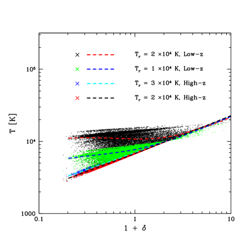
Figure 9.— Temperature density relation at $z=5.5$ for various reionization temperatures in the High-z and Low-z models. The “X”s in the legend indicate the color of the points in the corresponding models, while the dashed lines in the same models have different colors to promote visibility. The models in the legend are listed from top to bottom: the highest points and line (indicating the median temperature at various densities) show the $T_{r}=2\times 10^{4}$ K, Low-z model; next is the $T_{r}=1\times 10^{4}$ K, Low-z model; then the $T_{r}=3\times 10^{4}$ K, High-z model; and finally the $T_{r}=3\times 10^{4}$ K, High-z model.

Another perspective is to construct scatter plots in the temperature-density plane and plot median temperature-density relations for various models, as in Fig. 5 and Fig. 6. This is shown for gas at $z=5.5$ in Fig. 9. Consider first the two High-z models (the bottom two sets of points and dashed lines in the figure), which show the results of assuming $T_{r}=2\times 10^{4}$ K (bottom-most case with red points and a black dashed line), and $T_{r}=3\times 10^{4}$ K (shown as blue points and a cyan line, just above the bottom-most model). This shows that the results in this model are insensitive to $T_{r}$: this is as anticipated from Fig. 8. The next model is a Low-z case and has $T_{r}=1\times 10^{4}$ K (green points and blue line). This model is clearly closer to the High-z reionization model than our fiducial Low-z case, which is shown in the figure as the upper most black points with red line fit. However, the median temperature at low density and the scatter in the temperature are both larger in the Low-z, low reionization temperature model than in the High-z models. If the scatter in the temperature, and the trend of temperature with density can be measured observationally, this may help break the partial degeneracies between reionization redshift and temperature.

5. Measuring the Temperature of the $z\sim 5$ IGM

We now turn to consider the impact of the thermal state of the IGM on the properties of the $z\sim 5$ Ly-$\alpha$ forest, and on the possibility of extracting these signatures to learn about reionization. The effects of temperature on the statistics of the Ly-$\alpha$ forest are discussed, for example, in Lidz et al. (2010). The three main effects are: higher temperatures produce more Doppler broadening; the recombination rate of the absorbing gas is temperature dependent with hotter gas recombining more slowly, leading to less neutral gas and less absorption; hotter gas leads to more Jeans smoothing, with the precise impact of this smoothing depending on the entire prior thermal history of the absorbing gas (Gnedin & Hui, 1998).

The enhanced Doppler broadening and Jeans smoothing in models with high temperatures each act to reduce the amount of small-scale structure in the Ly-$\alpha$ forest. These two effects are not, however, entirely degenerate: Jeans smoothing filters the gas distribution in three dimensions, while Doppler broadening smooths the optical depth field along the line of sight (e.g. Zaldarriaga et al. 2001). Previous studies suggest that Doppler broadening impacts the small scale structure in the forest more than Jeans smoothing, at least near $z\sim 3$ (Zaldarriaga et al., 2001; Peeples et al., 2010; Lidz et al., 2010). At $z\sim 5$, we expect Jeans smoothing to have more impact, however: the high opacity in the Ly-$\alpha$ line at these redshifts implies that even slight density enhancements can give rise to noticeable absorption lines, and these slight density variations may be erased by Jeans smoothing. Unfortunately, it is challenging to model the impact of Jeans smoothing while incorporating a realistic model for inhomogeneous reionization and photoheating. This requires hydrodynamic models that resolve the filtering scale, while capturing a large enough volume to model patchy reionization. Furthermore, the filtering scale depends on the entire prior thermal history. In this paper, we defer this challenge to future work and assume that the effect of Jeans smoothing is sub-dominant to that of Doppler broadening. We caution that Jeans smoothing might, however, enhance the impact of patchy reionization and modeling it may be necessary to robustly interpret future measurements.

In any case, the small-scale structure in the Ly-$\alpha$ forest should be sensitive to the thermal state and the thermal history of the IGM, and so we now consider an approach for estimating the amplitude of small-scale structure in the forest. Here we will use the basic technique described in Lidz et al. (2010), except applied here to simulated data at higher redshift where there is more absorption in the forest. The first issue we aim to explore here is to what extent the temperature of the IGM is measurable at higher redshift, where the forest is significantly more absorbed. A second goal is to explore the impact of the temperature inhomogeneities modeled in the previous section.

We briefly outline the approach of Lidz et al. (2010) for measuring the small-scale structure – and thereby extracting constraints on the IGM temperature – here for completeness. In this approach, each spectrum is convolved with a Morlet wavelet filter and the smoothing scale of this filter is tuned to extract the amplitude of the small scale power spectrum in the forest as a function of position across each spectrum. The Morlet filter is a plane wave, multiplied by a Gaussian and in configuration space may be written as:

$$\Psi_{n}(x)=K\rm{exp}(ik_{0}x)\rm{exp}\left[-\frac{x^{2}}{2s_{n}^{2}}\right].$$ (6)

The Fourier space counterpart, when the normalization constant $K$ is fixed so the filter has unit power (see Lidz et al. 2010) is:

$$\Psi_{n}(k)=\pi^{-1/4}\sqrt{\frac{2\pi s_{n}}{\Delta u}}\rm{exp}\left[-\frac{(k-k_{0})^{2}s_{n}^{2}}{2}\right].$$ (7)

In the above equation, $\Delta u$ is the size of each spectral pixel in velocity units and $s_{n}$ is a suitable smoothing scale (also in velocity units) chosen to extract the small scale power, and we set $k_{0}s_{n}=6$ (see Lidz et al. 2010). Each mock spectrum is convolved with the above filter. We work with the transmission fluctuation field, $\delta_{F}(x)=(F(x)-\langle F\rangle)/\langle F\rangle$ where $F=e^{-\tau}$ is the transmission and $\langle F\rangle$ is the ensemble-averaged mean transmitted flux.

The transmission fluctuation, convolved with the wavelet filter, is:

$$a_{n}(x)=\int dx^{\prime}\Psi_{n}(x-x^{\prime})\delta_{F}(x^{\prime}),$$ (8)

The amplitude of this filtered field, at position “$x$” is given by

$$A(x)=|a_{n}(x)|^{2},$$ (9)

and characterizes the amount of small-scale structure in the transmission field. We generally smooth this field with a top-hat of length $L$,

$$A_{L}(x)=\frac{1}{L}\int_{-\infty}^{\infty}dx^{\prime}\Theta(|x-x^{\prime}|;L/2)A(x^{\prime}),$$ (10)

where $\Theta$ is a top-hat function. The quantity $A_{L}(x)$ is a measure of the average small scale power across different portions of a quasar spectrum, and should broadly trace the temperature of corresponding regions in the IGM, with cold regions giving a larger $A_{L}$ than hot regions.

5.1. Hydrodynamic Simulations: Perfect Temperate-Density Relation Models

As a first test, we take high redshift outputs from the hydrodynamic simulation (see §2) and impose temperature-density relations before producing mock quasar spectra. This test ignores the impact of inhomogeneous reionization, but it nonetheless provides some intuition for how well our approach can constrain the IGM temperature.

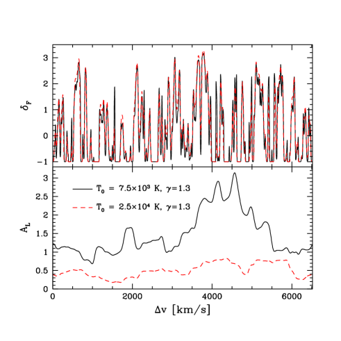
Figure 10.— Example sightlines and wavelet amplitudes for two different models of the IGM temperature at $z\sim 5$. The top panel shows $\delta_{F}(x)$ for an example sightlines with $T_{0}=2.5\times 10^{4}$ K, $\gamma=1.3$ (red dashed) and the same sightline except with $T_{0}=7.5\times 10^{3}$ K, $\gamma=1.3$ (black solid). The bottom panel shows the smoothed wavelet amplitudes, $A_{L}$, along each spectrum. The lower temperature model has more small scale structure and larger wavelet amplitudes. The smoothing scale $s_{n}=51$ km/s here, while $\Delta u=3.2$ km/s and $L=1,000$ km/s.

Fig. 10 shows an example sightline, $50$ Mpc/$h$ in length, extracted from the hydrodynamic simulation at $z=5$ for each of two different temperature-density relation models. The top panel shows the transmission fluctuation, $\delta_{F}$, for models with $\gamma=1.3$ and each of $T_{0}=7.5\times 10^{3}$ K and $T_{0}=2.5\times 10^{4}$ K while the bottom panel shows the smoothed wavelet amplitudes, $A_{L}$, in each model. In this case, the smoothing scale $s_{n}$ is set to $s_{n}=51$ km/s, the pixel size to $\Delta u=3.2$ km/s, and $L=1,000$ km/s. In each case the intensity of the ionizing background has been renormalized so that the global mean transmitted flux is $\langle F\rangle=0.20$. This is the mean transmitted flux implied by extrapolating the recent best-fit measurement of Becker et al. (2012) to $z=5$.

Although the differences between $\delta_{F}$ along the two example sightlines are generally small, there are some noticeable differences. In particular, it appears that the “spikes” of transmission in the colder model are more prominent. This is mostly a result of the larger Doppler widths in the hot model. At this redshift, the heights of the transmission spikes are often influenced by nearby gas elements that are centered on saturated or highly absorbed parts of the spectrum; the broad Doppler wings from this gas extend into adjoining unsaturated regions and thereby reduce the height of neighboring transmission spikes. The spikes are less impacted by the narrower Doppler wings in the colder model and remain more prominent. Essentially, the forest has become “inverted” at these redshifts in comparison to at lower redshift. At sufficiently low redshift, the forest is mostly transmitted with some prominent absorption lines interspersed. In the low redshift case most of the information about the IGM temperature comes from narrow absorption lines. At high redshift, the forest is mostly absorbed and most of the information about the IGM temperature is instead in the transmission spikes.

In either case, the amount of small scale power in the Ly-$\alpha$ forest is indicative of the temperature of the gas in the IGM. This is illustrated by the bottom panel of Fig. 10 for the high redshift case considered here. This panel shows the smoothed wavelet amplitudes along each line of sight. The smoothed wavelet amplitudes are larger in the cold IGM model, with the largest differences occurring near $\Delta v\sim 4500$ km/s, close to several prominent transmission spikes in the models.

One possible complication is that long completely saturated regions will – regardless of temperature – have low wavelet amplitudes, $A_{L}$, since there is no small scale structure in such regions. These saturated zones may in fact be more prominent in models with low temperature since cold regions recombine more quickly, and hence have larger neutral fractions and suffer more absorption than hot regions. Fig. 10 suggests, however, that this is not a big effect at $z=5$, $\langle F\rangle=0.2$, although the saturated regions will be more prominent at higher redshift (see §5.3). We can guard against “contamination” from saturated regions by masking them before measuring the probability distribution of the wavelet amplitudes, and by varying the smoothing scale $L$.

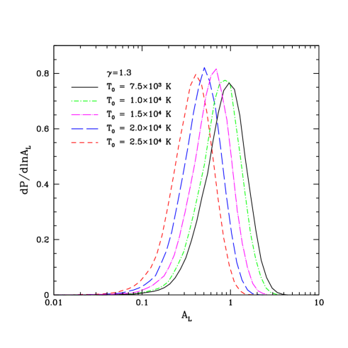
Figure 11.— Probability distribution of $A_{L}$ for various $T_{0}$ models at $z\sim 5$. Each model here assumes a perfect temperature density relation with $\gamma=1.3$, and in each case the mean transmitted flux has been fixed – by adjusting the intensity of the ionizing background – to $\langle F_{\alpha}\rangle=0.20$. As in Fig. 10, the smoothing scale has been set to $s_{n}=51$ km/s, while $\Delta u=3.2$ km/s and $L=1,000$ km/s.

To characterize the variations of the wavelet amplitudes with temperature more quantitatively, we calculate the probability distribution function (PDF) of wavelet amplitudes for ensembles of mock spectra generated from different temperature-density relation models. The results of these calculations are shown in Fig. 11. The PDF is quite sensitive to the temperature at mean density in these models. For example, the location of the peak in the wavelet amplitude PDF is at an $A_{L}$ that is roughly three times larger in the coldest model shown (with $T_{0}=7.5\times 10^{3}$ K), compared to the hottest model considered here ($T_{0}=2.5\times 10^{4}$ K). For the mean transmitted flux ($\langle F\rangle=0.20$) and $z=5$, the wavelet PDF for $s_{n}=51$ km/s is sensitive mostly to densities near the cosmic mean. As a result, we find that the wavelet PDFs here depend strongly on $T_{0}$, but are insensitive to $\gamma$, the slope of the temperature-density relation. It is hence important to keep in mind that our approach for measuring the IGM temperature is only sensitive to the temperature of the IGM close to the mean density, and it is therefore not possible to extract the full trend of temperature with density shown in our models (e.g., Fig. 5).

Although the PDFs depend sensitively on $T_{0}$, it is also clear that the wavelet amplitudes are not perfect indicators of the temperature. In the limit that the temperature at mean density were the only quantity that determined $A_{L}$, these PDFs should approach delta functions in $A_{L}$. That the wavelet PDFs have some breadth is not, however, surprising: the temperature is clearly not the only quantity that determines the small-scale structure in the forest. That said, Fig. 11 looks promising and helps to motivate further study.

5.2. Degeneracy with the Mean Transmitted Flux

One other potential issue, however, is that the wavelet PDF is also sensitive to the somewhat uncertain value of the mean transmitted flux, $\langle F\rangle$. Although the present statistical uncertainties on this quantity are $\sigma_{\langle F\rangle}/\langle F\rangle\leq 10\%$ near $z\sim 5$ (Becker et al. 2012), the systematic uncertainties are significantly larger. In particular, it is difficult to estimate the unabsorbed quasar continuum level, especially at the redshifts of interest for this study, where the absorption in the forest is very large (e.g. Faucher-Giguère et al. 2008). The measurement of the wavelet PDF itself should, however, be fairly robust to uncertainties in the level of the unabsorbed quasar continuum. This is the case because we consider the statistics of the transmission fluctuations, $\delta_{F}=(F-\langle F\rangle)/\langle F\rangle$, for which a (multiplicative) error in the continuum normalization divides out (see Lidz et al. (2010) for a discussion and tests with lower redshift data).

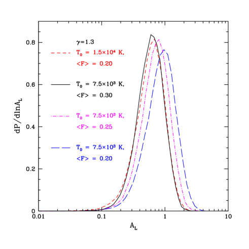
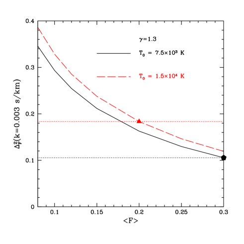
Figure 12.— Degeneracy with $\langle F\rangle$. Top panel: Although the PDF of $A_{L}$ is sensitive to $T_{0}$, this effect is degenerate with the impact of varying $\langle F\rangle$. For instance, the model with $T_{0}=1.5\times 10^{4}$ K and $\langle F\rangle=0.20$ is closely mimicked by a colder model with $T_{0}=7.5\times 10^{3}$ K, yet a larger mean transmission of $\langle F\rangle=0.30$. Bottom panel: This illustrates that the degeneracy can be broken by measuring the (relatively) large scale flux power spectrum. The curves here show the flux power spectrum, evaluated at a single convenient (larger-scale) wavenumber of $k=0.003$ s/km, in each $T_{0}$ model as a function of $\langle F\rangle$. The triangle and pentagon show the flux power for each model at the $\langle F\rangle$ for which the wavelet amplitude PDFs are degenerate in the two models. The large scale flux power in these two models differs appreciably and can be used to break the degeneracy. The red dotted and black dotted horizontal lines are intended only to guide the eye.

Nevertheless, we still need to know the mean transmitted flux very accurately: we use this measurement to in turn fix the intensity of the ionizing background at the redshifts of interest, which is itself quite uncertain. The amount of small scale structure in the forest, and hence the model wavelet amplitudes, do depend on the overall mean transmitted flux. As a result, while we should be able to measure the wavelet PDF without knowing the precise continuum normalization, our interpretation of this measurement still requires knowing the mean transmitted flux. To illustrate this, we plot (in the top panel of Fig. 12) the $z=5$ wavelet amplitude PDF in a model with $T_{0}=1.5\times 10^{4}$ K and the preferred mean transmitted flux at this redshift ($\langle F\rangle=0.20$, red short-dashed line). As in Fig. 11, the wavelet amplitudes are smaller in this model than in, for example, the cooler model with $T_{0}=7.5\times 10^{3}$ K at the same value of the mean transmitted flux (blue long-dashed line in the top panel of Fig. 12). However, if we allow the mean transmitted flux to increase in the colder model, the resulting wavelet PDF becomes similar to that in the hotter model. In particular, the black solid line shows a colder model with the mean transmitted flux increased to $\langle F\rangle=0.30$; this closely matches the wavelet PDF in the hotter model at the smaller mean transmitted flux ($\langle F\rangle=0.20$). This particular value of the mean transmitted flux, $\langle F\rangle=0.30$, is well outside the presently allowed range, given the statistical errors on current measurements. Nevertheless, the wavelet PDF clearly shows some degeneracy between variations in $T_{0}$ and in $\langle F\rangle$. This invites further attention, especially given the systematic concerns associated with estimating the unabsorbed continuum level.

One way to help break this degeneracy is to combine the measured wavelet PDF with a measurement of the flux power spectrum on larger scales. This quantity is especially sensitive to the mean transmitted flux, and the power spectrum of $\delta_{F}$ has the virtue – like the wavelet PDF – that it is insensitive to the overall normalization of the quasar continuum. On the other hand, on sufficiently large scales, the gentle fluctuations in the underlying quasar continuum still likely contaminate this measurement. However, there should still be a useful range of scales where the structure in the forest dominates over that in the continuum (see e.g. McDonald et al. 2006) and it is these scales that we will consider to help break the $T_{0}-\langle F\rangle$ degeneracy.

To illustrate how the flux power measurement may help break this degeneracy, we plot the amplitude of transmission fluctuations, $\Delta^{2}_{F}=kP_{F}(k)/\pi$, for a single example wavenumber ($k=0.003$ s/km in velocity units, or $k=0.39h$ Mpc^-1 in co-moving units at $z=5$) as a function of mean transmitted flux. The 1-D flux power spectrum ($P_{F}(k)$) is fairly flat on large scales and so the precise $k$ considered here is not especially important. The bottom panel of Fig. 12 shows the flux power spectrum at $k=0.003$ s/km as a function of $\langle F\rangle$ for the two values of $T_{0}$. In each case, $\Delta^{2}_{F}$ is a strong function of $\langle F\rangle$. The red triangle and black pentagon show the power spectra in the $T_{0}=1.5\times 10^{4}$ K and the $T_{0}=7.5\times 10^{3}$ K models respectively, for the values of the mean transmitted flux ($\langle F\rangle=0.20$ and $\langle F\rangle=0.30$) at which their wavelet PDFs are degenerate. The large scale flux power spectra in these two models differ by the sizable factor of $1.7$. It should be straightforward to measure the flux power spectrum on these scales to this level of accuracy, and so this measurement can help pin down $\langle F\rangle$ and break the degeneracy.

One possible concern with this approach is that the precise relationship between $\Delta^{2}_{F}$ and $\langle F\rangle$ may be somewhat model dependent, and our inability to perfectly model the forest – especially at high redshifts, potentially close to the EoR – might lead us to draw spurious conclusions. At present, the only way to guard against this possibility is to test the goodness-of-fit of our models for as wide a range of empirical tests as possible. Ideally, one would compare models with measurements of the flux power across a wide range of scales (although significantly larger scales will be subject to contamination from power in the quasar continuum), the wavelet PDF, the mean transmitted flux, and perhaps the statistics of the Ly-$\beta$ forest as well (e.g. Dijkstra et al. 2004; Furlanetto & Oh 2009).

5.3. Wavelet Amplitude PDFs in Inhomogeneous Reionization Models

With the results of the previous section as a guide, we now turn to consider the wavelet amplitude PDFs in the more realistic inhomogeneous temperature models developed in §4. In this case, we are using the dark matter simulations of McQuinn et al. (2007a) along with our model temperature distributions. Although the large volume of these simulations allows us to capture the reionization-induced inhomogeneities, they are not – taken as is – adequate for capturing the small-scale structure in the Ly-$\alpha$ forest, which is the basic observable we aim to explore here.

In order to make headway, we add small-scale structure to sightlines extracted from the simulation cube using the log-normal model, as in Kohler et al. (2007). Briefly, we generate one-dimensional Gaussian random fields $\delta_{G}$ using the one-dimensional linear density power spectrum (scaled to the redshift of interest, and calculated after smoothing the three-dimensional linear power spectrum with a filter of the form $e^{-2k^{2}/k_{f}^{2}}$ and $k_{f}=30h$ Mpc^-1 to loosely mimic the effect of Jeans smoothing, Gnedin & Hui 1998). From the Gaussian random realizations, we produce lognormal fields at high resolution using the transformation $1+\delta_{\rm LN}=e^{\delta_{G}-\sigma_{G}^{2}/2}$, where $\sigma_{G}^{2}$ is the variance of the Gaussian random field. As in Kohler et al. (2007) the lognormal field is modulated by the larger scale modes captured in the simulation ($\delta_{\rm sim}$) according to $1+\delta=(1+\delta_{\rm sim})(1+\delta_{\rm LN})$ with the (subscript-free) symbol $\delta$ denoting the density contrast with added small-scale structure. Similarly, using the simulated temperature in a coarse pixel (described by $T_{0}$ and $\gamma$), the temperature in a fine pixel becomes $T=T_{0}(1+\delta)^{\gamma-1}$.

The main disadvantage here is that the resulting sightlines have too much large scale structure: the lognormal field adds both large and small scale modes to the simulation, and the simulation was not deficient in large scale power to begin with. This is partly mitigated by our using a slightly higher redshift simulation output ($z=6.9$) than the redshift of interest. This simple approach is hence imperfect, but the added small scale structure does nevertheless allow us to reliably model the impact of thermal broadening on the resulting mock Ly-$\alpha$ forest spectra. As a test, we measure the flux power spectrum from the mock “lognormal-enhanced” sightlines and compare them with the flux power spectrum from mock spectra generated from the hydrodynamic simulation. The flux power spectrum from the lognormal spectra is roughly $50\%$ larger than from the hydrodyamic simulations. However, the overall shape of the flux power is fairly well captured in the lognormal case, and importantly, the shape of the flux power spectrum varies in a similar way in both calculations as the temperature and thermal broadening are varied. Hence we believe that this approach suffices to capture the main impact of patchy reionization on the small scale structure in the Ly-$\alpha$ forest. We caution, however, that a detailed comparison with upcoming measurements will certainly require improvements here.

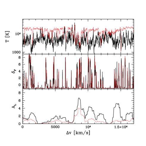
Figure 13.— Example sightlines and wavelet amplitudes from the Low-z and High-z reionization models. In the models here, the global mean flux is $\langle F\rangle=0.1$ and $z=5.5$. In each panel the red dotted line shows a sightline through the $T_{r}=3\times 10^{4}$ K, Low-z reionization model while the black solid line is the same sightline, except in this case the temperature field is drawn from the High-z reionization model (with $T_{r}=2\times 10^{4}$ K). The simulated density and temperature fields have small scale structure added according to the lognormal model, as described in the text. Top panel: The simulated temperature field. Middle panel: The transmission field, $\delta_{F}$. Bottom panel: The smoothed wavelet amplitude with $L=1,000$ km/s, $s_{n}=34$ km/s, and $\Delta u=2.1$ km/s. The transmission fluctuations and wavelet amplitudes are larger than in Fig. 10, mostly because of the lower mean transmitted flux adopted here.

With this cautionary remark, we turn to consider the properties of mock spectra drawn from our inhomogeneous temperature models. Fig. 13 shows typical example sightlines from the High-z and Low-z reionization models at $z=5.5$ and $\langle F\rangle=0.1$. The trends are broadly similar to those in Fig. 10: the colder models have more small scale structure than the hotter models. As a result, the transmission field has more prominent spikes in the colder High-z model, and the smoothed wavelet amplitudes in this model (bottom panel) are larger than in the Low-z model. The inhomogeneous models incorporate, however, the reionization-induced temperature variations that are not included in the previous model, although the impact of these variations are generally hard to discern by eye. One can however identify that the prominent cold region in the middle of this sightline, for example, corresponds to a pronounced peak in the smoothed wavelet amplitude field in each model. Note that the wavelet amplitudes and $\delta_{F}$ fluctuations are larger here than in Fig. 10 because here we consider $z=5.5$ and $\langle F\rangle=0.1$, while in the previous figure we considered $z=5.0$ and $\langle F\rangle=0.2$. In addition, the lower transmitted flux considered here leads to more completely absorbed regions in the mock Ly-$\alpha$ forest, and these regions have correspondingly low wavelet amplitudes. As discussed earlier, these regions do not contain information about the IGM temperature.

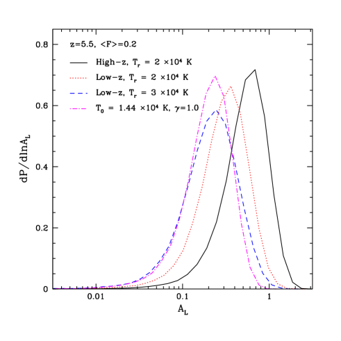
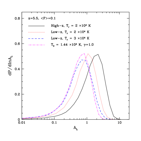
Figure 14.— Probability distribution of $A_{L}$ for various reionization and temperature models at $z=5.5$. Top panel: In this panel all models are normalized to $\langle F\rangle=0.2$. The solid black curve shows the wavelet amplitudes for the High-z reionization model (with $T_{r}=2\times 10^{4}$ K), while the red dotted and blue dashed curves show Low-z reionization models with reionization temperatures of $T_{r}=2\times 10^{4}$ K and $T_{r}=3\times 10^{4}$ K respectively. The magenta dot-dashed line shows a homogeneous temperature model for comparison. In this case, the temperature was set to match the median temperature in the Low-z, $T_{r}=3\times 10^{4}$ K model for gas at the cosmic mean density; the broader distribution in the Low-z model reflects the impact of inhomogeneous reionization. Bottom panel: Identical to the top panel, but here the models fix $\langle F\rangle=0.1$. In each case, the filter scale and pixel size are set to $s_{n}=34$ km/s and $\Delta u=2.1$ km/s respectively, while $L=1,000$ km/s.

More quantitatively, the resulting wavelet amplitude PDFs for some example inhomogeneous temperature models are shown in Fig. 14. Since the mean transmitted flux at this redshift ($z=5.5$) is somewhat uncertain, we compare models normalized to each of $\langle F\rangle=0.2$ (top panel) and $\langle F\rangle=0.1$ (bottom panel) in order to illustrate the impact of varying $\langle F\rangle$. Extrapolating the best fit measurement from (Becker et al., 2012), we find $\langle F\rangle=0.13$ at $z=5.5$ so this range should approximately bracket the expected value, although the lower end of this range is preferred. Note that there is some evidence that the mean transmitted flux decreases more rapidly above $z\sim 5.5$ or so compared to the evolution expected from lower redshifts (e.g. Fan et al. 2006), and so this would further favor the lower value, and perhaps even slightly smaller numbers than considered here. Nevertheless, it is worth considering the mean transmitted flux dependence explicitly: even if $\langle F\rangle=0.2$ is reached at $z=5$ rather than $z=5.5$, the temperature fluctuations could be as large at $z=5$ as in our $z=5.5$ models if reionization is more extended than considered here.

In each case, the wavelet filter’s smoothing scales are set to $s_{n}=34$ km/s and $L=1,000$ km/s, while the pixel size is $\Delta u=2.1$ km/s. In each panel, the PDF in the High-z model is compared to Low-z models for two different reionization temperatures, $T_{r}=2\times 10^{4}$ K and $T_{r}=3\times 10^{4}$ K. In addition, we plot the wavelet amplitude PDF for a model with a completely homogeneous temperature field. In this isothermal case the temperature is set to $T_{0}=1.44\times 10^{4}$ K, matching the median temperature near the cosmic mean density in the Low-z, $T_{r}=3\times 10^{4}$ K model. Homogeneous reionization models with the same $T_{0}$ but differing $\gamma$ would give very similar results, since the wavelet amplitudes are sensitive to absorbing gas near the cosmic mean density for these values of the mean transmitted flux. Comparing the $T_{0}=1.44\times 10^{4}$ K isothermal model with the Low-z, $T_{r}=3\times 10^{4}$ K case helps to illustrate the impact of temperature inhomogeneities.

First, we consider how the location of the peak in the PDF varies with the reionization model. The qualitative behavior is as expected: the High-z model peaks at the largest wavelet amplitude, while the Low-z models peak at smaller wavelet amplitude. This results because the High-z model is colder than the Low-z models, and so it has more small-scale structure and hence higher wavelet amplitudes. The Low-z model with the higher reionization temperature, $T_{r}=3\times 10^{4}$ K, has hotter gas at the redshift of interest ($z=5.5$) than in the Low-z scenario with $T_{r}=2\times 10^{4}$ K and so the PDF in the former model is peaked at smaller wavelet amplitudes.

These trends occur in both the $\langle F\rangle=0.1$ and $\langle F\rangle=0.2$ models. In the smaller $\langle F\rangle$ model the PDFs peak at larger $A_{L}$, reflecting the enhanced power in the $\delta_{F}=(F-\langle F\rangle)/\langle F\rangle$ field for decreasing mean flux. To provide a quantitative comparison, the High-z model has an average wavelet amplitude that is $73\%$ larger than in the Low-z, $T_{r}=2\times 10^{4}$ K model, while the average amplitude in the $T_{r}=3\times 10^{4}$ K, Low-z model is $27\%$ smaller than the $T_{r}=2\times 10^{4}$ K case. These numbers are for $\langle F\rangle=0.2$, but the fractional differences are similar for $\langle F\rangle=0.1$.

Next we consider the width of the wavelet amplitude PDFs. The width arises in part because $A_{L}$ is not a perfect tracer of temperature, and also because the temperature field is inhomogeneous. The latter contribution to the width can in principle be used to constrain the spread in the timing of reionization, and so this quantity is highly interesting. Comparing first the inhomogeneous models in Fig. 14, it is clear that the Low-z, $T_{r}=3\times 10^{4}$ K model has the widest distribution of wavelet amplitudes, followed by the Low-z, $T_{r}=2\times 10^{4}$ K model, while the High-z model has the narrowest $A_{L}$ distribution of these models. This is expected, since the High-z model has the smallest temperature fluctuations, while the Low-z, $T_{r}=3\times 10^{4}$ K model has the largest temperature fluctuations. It is also instructive to compare the isothermal models (magenta dot-dashed lines in each panel) with the Low-z, $T_{r}=3\times 10^{4}$ K models. The isothermal model has the same median temperature near the cosmic mean density as the Low-z, $T_{r}=3\times 10^{4}$ K model. This PDF is similar, but narrower, than in the inhomogeneous temperature case. Quantitatively, the fractional width of the distribution, $\sigma_{A,L}/\langle A_{L}\rangle$, is $18\%$ larger in the Low-z, $T_{r}=3\times 10^{4}$ K model than in the homogeneous case at $\langle F\rangle=0.2$ and $11\%$ larger at $\langle F\rangle=0.1$. These relatively small differences seem challenging to extract, but are sufficiently interesting to merit further investigation.

5.4. Forecasts

Finally, we briefly forecast the significance at which various models may be distinguished using existing data samples. Here we will be content with rough estimates. For simplicity, we predict the expected error bar on only the first two moments of the wavelet amplitude PDF, and compare this to the difference between some of our models. We consider a sample of $N_{\rm los}$ independent spectra, and assume that each spectrum has sufficient $S/N$ so that we can estimate error bars in the sample variance limit – i.e., we work in the limit that photon noise from the night sky and the quasar itself, as well as instrumental noise, are negligible compared to sample variance (also termed “cosmic variance”). Our error budget hence reflects the scatter expected – given the large scale structure of the universe and the limited volume probed by our hypothetical survey – around the true value that would be obtained if we could average over an infinite volume.

It is instructive to first consider the type of quasar spectra that are required to measure the wavelet amplitudes in the sample variance limit. The first obvious requirement is that the spectral resolution needs to be high enough to resolve the thermal broadening scale, which is on the order of $\sim 10$ km/s. This can be achieved with, for example, Keck HIRES spectra which have a spectral resolution of FWHM $=6.7$ km/s. Spectra from the MIKE spectrograph on Magellan would partly resolve the thermal broadening scale: the resolution of these spectra is a factor of $\sim 2$ worse than HIRES (e.g. Becker et al. 2011a). Next, we consider the impact of photon and instrumental noise. In particular, we estimate the $S/N$ (at the continuum) per HIRES pixel at which the expected shot-noise is a small fraction of the average wavelet amplitude in plausible models. The mean wavelet amplitude from the noise should be roughly $\langle A_{\rm noise}\rangle\approx(N/S)^{2}/\langle F\rangle$ (Hui et al., 2001; Lidz et al., 2010). In order for the noise to be sub-dominant, we impose that the noise should be less than $10\%$ of the mean wavelet amplitude in our Low-z, $T_{r}=2\times 10^{4}$ K model at $\langle F\rangle=0.2$ (which has $\langle A\rangle=0.35$). This requires a $S/N\gtrsim 12$ at the continuum, per $2.1$ km/s HIRES pixel. This is a fairly stringent requirement for quasars at the high redshifts of interest for our proposed measurements, but this sensitivity has been reached already in previous work. We could likely make a less stringent requirement on the $S/N$ of the data sample: this would just necessitate careful shot-noise subtraction, and boost our error budget somewhat. Currently, we are aware of roughly $\sim 10$ HIRES spectra in the published literature at $z\sim 5-5.7$ that meet our $S/N$ and resolution criteria (e.g. Becker et al. 2011b). There are substantially larger numbers of lower resolution and $S/N$ spectra from the SDSS that could potentially be followed-up at higher resolution and sensitivity to improve the statistics here. For example, there are $36$ SDSS-DR7 quasars in the $z=[5.0,5.2]$ redshift bin of Becker et al. (2012).

We now proceed to estimate the sample variance errors. The first quantity of interest is the sightline-to-sightline scatter in the wavelet amplitudes, averaged over the entire Ly-$\alpha$ forest region of each quasar. We define $P_{A,L}(k)$ to be the power spectrum of the fluctuations in the wavelet amplitude after smoothing the amplitudes on scale $L$, i.e., the power spectrum of $\delta_{A,L}(x)=(A_{L}(x)-\langle A_{L}\rangle)/\langle A_{L}\rangle$. We relate the expected error bars to this power spectrum, and estimate them by measuring $P_{A,L}(k)$ from our simulated models. This approach has the advantage that we can approximately extrapolate $P_{A,L}(k)$ to scales beyond that of our simulation box and roughly account for missing large scale Fourier modes. This power spectrum of $\delta_{A,L}(x)$ is a four point function of the flux and is related to the power spectrum of $A(x)$ (the unsmoothed wavelet amplitude power spectrum) from Eqs. 9 and 10 by

$$P_{A,L}(k)=\left[\frac{\rm{sin}(kL/2)}{kL/2}\right]^{2}P_{A}(k).$$ (11)

This is just a filtered version of the wavelet amplitude power spectrum. From each independent sightline, we estimate the moments of the wavelet amplitude PDF by further averaging over a length scale $L_{\rm spec}$, comparable to the separation (in velocity units) between the Ly-$\alpha$ and Ly-$\beta$ emission lines from the quasar. Note the distinction between the two smoothing scales here: $L$ is the smoothing scale over which we are studying the wavelet amplitude variations, while $L_{\rm spec}$ is the scale over which we estimate the moments from each spectrum.

The formula for the sample variance for a single sightline is then (Lidz et al., 2010):

$$\frac{\sigma^{2}_{A,L}(L_{\rm spec})}{\langle A\rangle^{2}}=\int_{-\infty}^{\infty}\frac{dk^{\prime}}{2\pi}\left[\frac{\rm{sin}(k^{\prime}L_{\rm spec}/2)}{k^{\prime}L_{\rm spec}/2}\right]^{2}P_{A,L}(k^{\prime}).$$

(12)

In a sample of $N_{\rm los}$ independent Ly-$\alpha$ forest sightlines, the expected (1-$\sigma$) fractional error on $\langle A_{L}\rangle$ (in the sample variance limit) is:

$$\frac{\delta\langle A_{L}\rangle}{\langle A_{L}\rangle}=\frac{1}{\sqrt{N_{\rm los}}}\frac{\sigma_{A,L}(L_{\rm spec})}{\langle A_{L}\rangle}.$$ (13)

We can compare this estimate of the fractional error in the average wavelet amplitude with the difference between the average amplitudes in some of the models of the previous section.

Next, we want to consider the expected error bar on the second moment of the wavelet PDF. This second moment provides one diagnostic for the impact of temperature inhomogeneities from patchy reionization. We would like to check whether the variance of the $A_{L}$ distribution is broad enough to imply patchy reionization. This requires computing the “variance of the variance”; in particular, we want the variance of an estimate of $\sigma^{2}_{A,L}$ when this quantity is estimated from a sightline of length $L_{\rm spec}$. We calculate this quantity assuming that $A_{L}$ approximately obeys Gaussian statistics. In this case, one can show that the desired variance is:

$${\rm Var}[\sigma^{2}_{A,L}(L_{\rm spec})]= 2\langle A_{L}\rangle^{4}\int_{-\infty}^{\infty}\frac{dk^{\prime}}{2\pi}\left[\frac{\rm{sin}(k^{\prime}L_{\rm spec}/2)}{k^{\prime}L_{\rm spec}/2}\right]^{2}$$

$$\times\int_{-\infty}^{\infty}\frac{dk^{\prime\prime}}{2\pi}P_{A,L}(k^{\prime}-k^{\prime\prime})P_{A,L}(k^{\prime\prime})$$

$$+4\langle A_{L}\rangle^{4}\sigma^{2}_{A,L}(L_{\rm spec}).$$ (14)

The expected error on an estimate of $\sigma^{2}_{A,L}$ from a sample of $N_{\rm los}$ independent sightlines is then:

$$\frac{\delta\sigma^{2}_{A,L}}{\sigma^{2}_{A,L}}=\frac{1}{\sqrt{N_{\rm los}}}\frac{\sqrt{{\rm Var}[\sigma^{2}_{A,L}(L_{\rm spec})]}}{\sigma^{2}_{A,L}}.$$ (15)

We can now plug numbers into Eqs. 13 and 15 to estimate the ability of current samples to constrain some of our models. We assume that $N_{\rm los}=10$ sightlines are available for our study, and take $z=5.5$, $\langle F\rangle=0.2$ here. We assume the true model is the $T_{r}=3\times 10^{4}$ K, Low-z case and examine at what significance other models may be distinguished from this case. Conservatively, we assume that $L_{\rm spec}=2.5\times 10^{4}$ km/s; the velocity separation between the Ly-$\alpha$ and Ly-$\beta$ emission lines is $5.1\times 10^{4}$ km/s, and so our assumed value effectively masks-out half of the forest. While one will want to mask-out proximity regions, damped Ly-$\alpha$ systems, prominent metal lines, etc., our choice is certainly conservative. In this case, evaluating Eq. 13 in our assumed true model, we find that a measurement of $\langle A_{L}\rangle$ from $N_{\rm los}=10$ sightlines should rule out the High-z ($T_{r}=2\times 10^{4}$ K) model at $32-\sigma$, and a Low-z model with the lower reionization temperature ($T_{r}=2\times 10^{4}$ K) at $9-\sigma$! These forecasts are optimistic, since we have assumed – for example – perfect knowledge of the mean transmitted flux; in practice, the mean transmitted flux may have to be constrained separately from the large-scale flux power spectrum (§5.2). Nonetheless, we believe the overall point is robust: existing samples should provide interesting constraints on $\langle A_{L}\rangle$.

Significantly more challenging is to measure the variance of the $A_{L}$ distribution well enough to identify signatures of patchy reionization. With the optimistic “true” model considered here (the Low-z, $T_{r}=3\times 10^{4}$ K case), however, we forecast that $N_{\rm los}=10$ spectra are sufficient to rule out the homogeneous $T=1.44\times 10^{4}$ K model at $2.4-\sigma$, based on the variance of the $A_{L}$ distribution alone. Note that both of these estimates assumed $\langle F\rangle=0.2$ and our $z=5.5$ temperature models but the expected constraints are similar for $\langle F\rangle=0.1$.

6. Conclusions

In this work, we modeled the temperature of the IGM at $z\gtrsim 5$, incorporating the impact of spatial variations in the timing of reionization across the universe. We contrasted the $z\sim 5$ temperature in models where reionization completes at high redshift – near $z=10$ – with scenarios where reionization completes later, near $z=6$. In agreement with previous work (Trac et al., 2008; Furlanetto & Oh, 2009), we found that the properties of the $z=5$ temperature differ markedly between these two models. The IGM is cooler in the early reionization model, and the usual temperature-density relation is a good description of the temperature state in this case, while the temperature state is more complex and inhomogeneous in the late reionization scenario.

We then produced mock $z\gtrsim 5$ Ly-$\alpha$ forest spectra from our numerical models, in effort to explore the observable implications of the IGM temperature as close as possible to hydrogen reionization. In particular, we used the Morlet wavelet filter approach of Lidz et al. (2010) to extract the small-scale structure across each Ly-$\alpha$ forest spectrum. The small-scale structure in the forest is sensitive to the temperature of the IGM, and the filter we use is localized in configuration space, which makes it well-suited for application in cases where the temperature field is inhomogeneous.

Interestingly, we found that the small-scale structure in the forest is sensitive to the IGM temperature even when the forest is highly absorbed. In particular, the transmission field in between absorbed regions is more spiky if the IGM is cold, compared to hotter models. Using existing high resolution Ly-$\alpha$ forest samples, one should be able to use this difference to distinguish between high redshift and lower redshift reionization models at high significance. It may, however, be necessary to combine measurements of the small-scale structure in the forest with measurements of the larger scale flux power spectrum to help break degeneracies with the mean transmitted flux, which is hard to estimate directly at the high redshifts of interest for these studies.

In addition, we considered the impact of spatial variations in the timing of reionization on the width of the wavelet amplitude distribution. We found that these variations broaden the width of this distribution, but that the broadening is fairly subtle. This likely results in part because the temperature variations we are interested in are coherent on rather large scales, and aliasing – from fluctuations in the transmission field transverse to the line of sight – obscures our ability to measure large scale fluctuations along the line of sight (e.g. McQuinn et al. 2011a; Lai et al. 2006). Nonetheless, we forecast that our Low-z, $T_{r}=3\times 10^{4}$ K model can be distinguished from a homogeneous temperature model at $2-3\sigma$ with existing samples of ten high resolution sightlines. Larger samples could improve on this, and an analysis of the small-scale structure in the Ly-$\beta$ forest might help as well. In this paper, we focused on the small-scale structure since it is a direct indicator of the temperature, but another approach would be to consider instead transmission fluctuations on large scales, especially as probed in “3D” measurements of the Ly-$\alpha$ forest (e.g. McQuinn et al. 2011a). This may be possible at $z\gtrsim 4$ with DESI (Levi et al., 2013; McQuinn et al., 2011a).

To robustly interpret future measurements, our modeling should be improved in various ways. In particular, we should incorporate inhomogeneous Jeans smoothing effects into our modeling. This might be accomplished by, for example, incorporating our semi-numeric modeling on top of a large dynamic range HPM (Gnedin & Hui, 1998) simulation. These calculations will need to face the competing requirements of capturing the large-scale variations in the timing of reionization, while simultaneously resolving the filtering scale. Nevertheless, we believe that measurements of the $z\gtrsim 5$ IGM temperature should provide a valuable handle on the reionization history of the universe.

Appendix: Approximate Thermal History Calculations

Here we derive an approximate analytic formula for the thermal history of an IGM gas element using linear perturbation theory. Here our derivation is quite similar to the analytic calculation in Hui & Gnedin (1997) (their §3.1), except here we include Compton cooling off of the CMB, which is important for our application in which we consider high redshift reionization and the temperature at redshifts close to reionization.

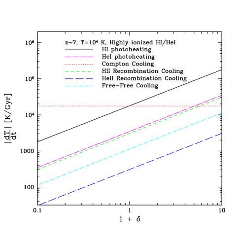
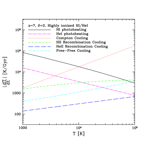
Figure 15.— Heating/cooling rates at $z\sim 7$. Left panel: The (absolute value of) the rates for relevant processes in the IGM at $T=10^{4}$ K as a function of density, assuming that hydrogen is highly ionized and that helium is mostly singly-ionized. Right panel: Similar to the left panel except the rates are shown as a function of temperature for gas at the comic mean density.

It is instructive to first briefly examine which heating/cooling processes are important, in addition to the usual adiabatic heating/cooling from the contraction/expansion of gas parcels. In particular, Fig. 15 compares the relative importance of HI photoheating, HeI photoheating, Compton cooling, HII recombination cooling, HeII recombination cooling, and free-free emission cooling for intergalactic gas at $z\sim 7$. The figure assumes that the gas is in ionization equilibrium and that hydrogen is highly ionized and helium mostly singly ionized. As in the body of the text, we are assuming that HeII reionization has not yet commenced at the redshifts of interest. For the highly-ionized and low density intergalactic gas considered here, line excitation cooling and collisional ionizations should be unimportant. The left hand panel considers the various heating and cooling processes for gas of fixed temperature, $T=10^{4}$ K, as a function of density while the right hand panel shows the same for gas at the comic mean density as a function of temperature. In each panel, the curves in the figure indicate the absolute values of the various rates, so that cooling processes are shown as positive numbers on the plot. The photoheating curves assume that the hardened ionizing spectrum follows a $J(\nu)\propto\nu^{-1.5}$ power-law near the photoionization edges. The dominant processes are clearly HI photoheating and Compton cooling. After these processes in importance are HeI photoheating and HII recombination cooling: these have rates that are roughly $20\%$ smaller than HI photoheating near the cosmic mean density and $T\sim 10^{4}$ K at $z\sim 7$. It is also interesting to note that at the densities considered here and for the adopted ionizing spectrum, HeI photoheating and HII recombination cooling have nearly equal magnitudes near $T\sim 10^{4}$ K; since these two processes enter the thermal evolution equation with opposite signs, this leads to a partial cancellation.

As a result, a good approximation to the IGM thermal evolution (at high redshifts before HeII reionization) results from including only adiabatic heating/cooling, Compton cooling, and HI photoheating. Note, however, that in the body of the work we include all of the additional processes considered in Fig. 15. The approximate results here are nonetheless useful and fairly accurate, and can in turn help to build intuition. The approximate equation for the thermal evolution is then:

$$\frac{dT}{dt}=-2HT+\frac{2T}{3(1+\delta)}\frac{d\delta}{dt}+\frac{\alpha_{0}\bar{n}_{e}E_{J}}{3(1+\chi_{\rm He})k_{B}}\left(\frac{T}{10^{4}K}\right)^{-0.7}(1+\delta)+\frac{4}{3}\frac{\sigma_{T}a_{\rm rad}T_{\gamma}^{4}}{m_{e}c}\left(T_{\gamma}-T\right).$$ (16)

Here $\alpha_{0}$ is the (case-A) recombination coefficient for hydrogen at $T=10^{4}$ K, $E_{J}$ is the average energy injected into the gas per photoionization, $T_{\gamma}$ is the CMB temperature (at the scale factor of interest), $\sigma_{T}$ is the Thomson scattering cross section, and $a_{\rm rad}T_{\gamma}^{4}$ is the energy density in the CMB. The first two terms describe adiabatic cooling/heating, the third term is from photoionization heating, and the last term accounts for Compton cooling. This equation assumes that the gas is in photoionization equilibrium, adopts an electron number density of $n_{e}=n_{H}+n_{He}$, and assumes the number density of free particles in the gas is $n_{\rm tot}=n_{e}+n_{H}+n_{He}=2(n_{H}+n_{He})$.

As in Hui & Gnedin (1997), we assume a solution of the form $T=T_{0}(1+\delta)^{\gamma-1}$ and linearize ($T\approx T_{0}[1+(\gamma-1)\delta]$) to find equations for $T_{0}$ and $\gamma-1$, as functions of scale factor. Let us first introduce two constants to make the notation more compact:

$${\mathcal{A}}=(10^{4}K)^{0.7}\frac{\alpha_{0}\bar{n}_{e}(0)E_{J}}{3(1+\chi_{\rm He})k_{B}H_{0}\sqrt{\Omega_{m}}}.$$ (17)

Here $\bar{n}_{e}(0)$ denotes the present day ($z=0$), spatially averaged, electron number density. Note that the constant ${\mathcal{A}}$ has dimensions of $[{\mathcal{A}}]=[K]^{1.7}$. In our fiducial model with $\alpha=1.5$, the numerical value of ${\mathcal{A}}$ is ${\mathcal{A}}=5.77\times 10^{5}K^{1.7}$. Second, we introduce

$${\mathcal{B}}=\frac{1}{H_{0}\sqrt{\Omega_{m}}t_{\rm Comp}(0)};\quad t_{\rm Comp}=\frac{3m_{e}c}{4\sigma_{T}a_{\rm rad}T_{\gamma}^{4}}.$$ (18)

Here $t_{\rm comp}(0)$ a characteristic timescale for Compton cooling today ($z=0$); this timescale falls off towards high redshift as $t_{\rm comp}\propto a^{4}$. In our assumed cosmology, the numerical value of this constant is ${\mathcal{B}}=1.15\times 10^{-2}$.

Using the high redshift approximation for the Hubble parameter, $H\approx H_{0}\sqrt{\Omega_{m}}a^{-3/2}$, and setting $\delta=0$ to find an equation for $T_{0}(a)$ valid in linear theory, Eq. 16 gives the following equation for $T_{0}$:

$$\frac{d(a^{2}T_{0})}{da}={\mathcal{A}}a^{0.9}(a^{2}T_{0})^{-0.7}-{\mathcal{B}}a^{-7/2}(a^{2}T_{0})+{\mathcal{B}}T_{\gamma}(0)a^{-5/2}.$$ (19)

A similar equation follows for $\gamma-1$ (again valid to linear order in $\delta$, and with the approximations to the thermal evolution equation in Eq. 16):

$$\frac{d(\gamma-1)}{da}=\left[\frac{2}{3}-(\gamma-1)\right]\frac{1}{a}+{\mathcal{A}}a^{0.9}(a^{2}T_{0})^{-1.7}\left[1-1.7(\gamma-1)\right]-\frac{{\mathcal{B}}T_{\gamma}(0)}{a^{2}T_{0}}a^{-5/2}(\gamma-1).$$ (20)

We can safely neglect the third term in Eq. 19, and we find a solution for $T_{0}(a)$ of the form (with the initial condition that the gas element is ionized at scale factor $a_{r}$ to a temperature $T_{r}$):

$$u=u_{r}{\rm exp}\left[0.68{\mathcal{B}}a^{-5/2}-0.68{\mathcal{B}}a_{r}^{-5/2}\right]+0.68{\mathcal{A}}(0.68{\mathcal{B}})^{0.76}e^{0.68{\mathcal{B}}a^{-5/2}}\int_{t}^{t_{r}}dt^{\prime}t^{\prime-1.76}e^{-t^{\prime}}.$$

$$u=(a^{2}T_{0})^{1.7};\quad u_{r}=(a_{r}^{2}T_{r})^{1.7};\quad t=0.68{\mathcal{B}}a^{-5/2};\quad t_{r}=0.68{\mathcal{B}}a_{r}^{-5/2}.$$ (21)

The corresponding solution to Eq. 20 for the evolution of $\gamma$ does not have a simple closed analytic form, but the equations can be solved numerically. Comparing the solutions for $T_{0}(z)$ from Eq. 21 and $\gamma(z)$ from Eq. 20 with results given in the body of the text, we find that the approximate solutions are good to better than $10\%$ accuracy. This accuracy is, in fact, somewhat better than might be expected given the approximations made, and may reflect cancelations between some of the neglected terms (such as the compensating omissions of HeI photoheating and HII recombination cooling, as highlighted in Fig. 15). Nevertheless, the approximate solutions seem quite useful and so we include them here.

References

- Abel & Haehnelt (1999) Abel, T., & Haehnelt, M. G. 1999, Astrophys.J., 520, L13, astro-ph/9903102
- Ade et al. (2013) Ade, P., et al. 2013, 1303.5076
- Becker et al. (2011a) Becker, G. D., Bolton, J. S., Haehnelt, M. G., & Sargent, W. L. 2011a, Mon.Not.Roy.Astron.Soc., 410, 1096, 1008.2622
- Becker et al. (2012) Becker, G. D., Hewett, P. C., Worseck, G., & Prochaska, J. X. 2012, 1208.2584
- Becker et al. (2011b) Becker, G. D., Sargent, W. L., Rauch, M., & Calverley, A. P. 2011b, Astrophys.J., 735, 93, 1101.4399
- Becker et al. (2001) Becker, R. H., et al. 2001, Astron.J., 122, 2850, astro-ph/0108097
- Bennett et al. (2013) Bennett, C., et al. 2013, Astrophys.J.Suppl., 208, 20, 1212.5225
- Bertschinger & Jain (1994) Bertschinger, E., & Jain, B. 1994, Astrophys.J., 431, 486, astro-ph/9307033
- Bolton et al. (2011) Bolton, J. S., Becker, G. D., Raskutti, S., Wyithe, J. S. B., Haehnelt, M. G., et al. 2011, 1110.0539
- Cen et al. (2009) Cen, R., McDonald, P., Trac, H., & Loeb, A. 2009, Astrophys.J., 706, L164, 0907.0735
- Chang et al. (2012) Chang, P., Broderick, A. E., & Pfrommer, C. 2012, Astrophys.J., 752, 23, 1106.5504
- Croft et al. (2002) Croft, R. A., Weinberg, D. H., Bolte, M., Burles, S., Hernquist, L., et al. 2002, Astrophys.J., 581, 20, astro-ph/0012324
- Dijkstra et al. (2004) Dijkstra, M., Lidz, A., & Hui, L. 2004, Astrophys.J., 605, 7, astro-ph/0305498
- Doroshkevich (1970) Doroshkevich, A. G. 1970, Astrofizika, 6, 581
- Fan et al. (2006) Fan, X.-H., Strauss, M. A., Becker, R. H., White, R. L., Gunn, J. E., et al. 2006, Astron.J., 132, 117, astro-ph/0512082
- Faucher-Giguère et al. (2008) Faucher-Giguère, C.-A., Prochaska, J. X., Lidz, A., Hernquist, L., & Zaldarriaga, M. 2008, ApJ, 681, 831, 0709.2382
- Furlanetto & Oh (2009) Furlanetto, S., & Oh, S. P. 2009, 0901.1888
- Furlanetto et al. (2004) Furlanetto, S., Zaldarriaga, M., & Hernquist, L. 2004, Astrophys.J., 613, 1, astro-ph/0403697
- Gnedin & Hui (1998) Gnedin, N. Y., & Hui, L. 1998, Mon.Not.Roy.Astron.Soc., 296, 44, astro-ph/9706219
- Gunn & Peterson (1965) Gunn, J. E., & Peterson, B. A. 1965, ApJ, 142, 1633
- Hui et al. (2001) Hui, L., Burles, S., Seljak, U., Rutledge, R. E., Magnier, E., et al. 2001, Astrophys.J., 552, 15, astro-ph/0005049
- Hui & Gnedin (1997) Hui, L., & Gnedin, N. Y. 1997, Mon.Not.Roy.Astron.Soc., 292, 27, astro-ph/9612232
- Hui & Haiman (2003) Hui, L., & Haiman, Z. 2003, Astrophys.J., 596, 9, astro-ph/0302439
- Hui et al. (2000) Hui, L., Kofman, L., & Shandarin, S. F. 2000, Astrophys.J., 537, 12, astro-ph/9901104
- Kohler et al. (2007) Kohler, K., Gnedin, N. Y., & Hamilton, A. J. S. 2007, ApJ, 657, 15, astro-ph/0511627
- Kuhlen & Faucher-Giguere (2012) Kuhlen, M., & Faucher-Giguere, C. 2012, 1201.0757
- Lai et al. (2006) Lai, K., Lidz, A., Hernquist, L., & Zaldarriaga, M. 2006, Astrophys.J., 644, 61, astro-ph/0510841
- Levi et al. (2013) Levi, M., et al. 2013, 1308.0847
- Lidz et al. (2010) Lidz, A., Faucher-Giguere, C.-A., Dall’Aglio, A., McQuinn, M., Fechner, C., et al. 2010, Astrophys.J., 718, 199, 0909.5210
- Lidz et al. (2007) Lidz, A., McQuinn, M., & Zaldarriaga, M. 2007, Astrophys.J., 670, 39, astro-ph/0703667
- Madau et al. (1999) Madau, P., Haardt, F., & Rees, M. J. 1999, ApJ, 514, 648, arXiv:astro-ph/9809058
- McDonald et al. (2001) McDonald, P., Miralda-Escude, J., Rauch, M., Sargent, W. L., Barlow, T. A., et al. 2001, Astrophys.J., 562, 52, astro-ph/0005553
- McDonald et al. (2006) McDonald, P., et al. 2006, Astrophys.J.Suppl., 163, 80, astro-ph/0405013
- McGreer et al. (2011) McGreer, I. D., Mesinger, A., & Fan, X. 2011, 1101.3314
- McQuinn (2012) McQuinn, M. 2012, Mon.Not.Roy.Astron.Soc., 426, 1349, 1206.1335
- McQuinn et al. (2011a) McQuinn, M., Hernquist, L., Lidz, A., & Zaldarriaga, M. 2011a, Mon.Not.Roy.Astron.Soc., 415, 977, 1010.5250
- McQuinn et al. (2007a) McQuinn, M., Hernquist, L., Zaldarriaga, M., & Dutta, S. 2007a, Mon.Not.Roy.Astron.Soc., 381, 75, 0704.2239
- McQuinn et al. (2007b) McQuinn, M., Lidz, A., Zahn, O., Dutta, S., Hernquist, L., et al. 2007b, Mon.Not.Roy.Astron.Soc., 377, 1043, astro-ph/0610094
- McQuinn et al. (2009) McQuinn, M., Lidz, A., Zaldarriaga, M., Hernquist, L., Hopkins, P. F., et al. 2009, Astrophys.J., 694, 842, 0807.2799
- McQuinn et al. (2011b) McQuinn, M., Oh, S. P., & Faucher-Giguere, C.-A. 2011b, Astrophys.J., 743, 82, 1101.1964
- Mesinger (2009) Mesinger, A. 2009, 0910.4161
- Miralda-Escude et al. (1996) Miralda-Escude, J., Cen, R.-y., Ostriker, J. P., & Rauch, M. 1996, Astrophys.J., 471, 582, astro-ph/9511013
- Miralda-Escudé & Rees (1994) Miralda-Escudé, J., & Rees, M. J. 1994, MNRAS, 266, 343
- Pawlik et al. (2008) Pawlik, A. H., Schaye, J., & van Scherpenzeel, E. 2008, 0807.3963
- Peeples et al. (2010) Peeples, M. S., Weinberg, D. H., Dave, R., Fardal, M. A., & Katz, N. 2010, Mon.Not.Roy.Astron.Soc., 404, 1295, 0910.0250
- Raskutti et al. (2012) Raskutti, S., Bolton, J. S., Wyithe, J. S. B., & Becker, G. D. 2012, 1201.5138
- Reisenegger & Miralda-Escude (1995) Reisenegger, A., & Miralda-Escude, J. 1995, ApJ, 449, 476, astro-ph/9502063
- Ricotti et al. (2000) Ricotti, M., Gnedin, N. Y., & Shull, J. M. 2000, Astrophys.J., 534, 41, astro-ph/9906413
- Robertson et al. (2013) Robertson, B. E., Furlanetto, S. R., Schneider, E., Charlot, S., Ellis, R. S., et al. 2013, Astrophys.J., 768, 71, 1301.1228
- Schaye et al. (2000) Schaye, J., Theuns, T., Rauch, M., Efstathiou, G., & Sargent, W. L. 2000, Mon.Not.Roy.Astron.Soc., 318, 817, astro-ph/9912432
- Shapiro & Giroux (1987) Shapiro, P. R., & Giroux, M. L. 1987, ApJ, 321, L107
- Sheth et al. (2001) Sheth, R. K., Mo, H., & Tormen, G. 2001, Mon.Not.Roy.Astron.Soc., 323, 1, astro-ph/9907024
- Springel (2005) Springel, V. 2005, MNRAS, 364, 1105, astro-ph/0505010
- Syphers et al. (2011) Syphers, D., Anderson, S. F., Zheng, W., Smith, B., Pieri, M., et al. 2011, Astrophys.J., 742, 99, 1108.4727
- Theuns et al. (2002a) Theuns, T., Schaye, J., Zaroubi, S., Kim, T.-S., Tzanavaris, P., et al. 2002a, Astrophys.J., 567, L103, astro-ph/0201514
- Theuns et al. (2002b) Theuns, T., Zaroubi, S., Kim, T.-S., Tzanavaris, P., & Carswell, R. F. 2002b, Mon.Not.Roy.Astron.Soc., 332, 367, astro-ph/0110600
- Trac et al. (2008) Trac, H., Cen, R., & Loeb, A. 2008, 0807.4530
- Viel et al. (2013) Viel, M., Becker, G. D., Bolton, J. S., & Haehnelt, M. G. 2013, Physical Review, D88, 043502, 1306.2314
- Worseck et al. (2011) Worseck, G., Prochaska, J. X., McQuinn, M., Dall’Aglio, A., Fechner, C., et al. 2011, Astrophys.J., 733, L24, 1103.5752
- Zahn et al. (2006) Zahn, O., Lidz, A., McQuinn, M., Dutta, S., Hernquist, L., et al. 2006, Astrophys.J., 654, 12, astro-ph/0604177
- Zaldarriaga et al. (2001) Zaldarriaga, M., Hui, L., & Tegmark, M. 2001, Astrophys.J., 557, 519, astro-ph/0011559
- Zel’dovich (1970) Zel’dovich, Y. B. 1970, A&A, 5, 84
- Zuo & Phinney (1993) Zuo, L., & Phinney, E. S. 1993, ApJ, 418, 28