Neutrino electromagnetic interactions: a window to new physics

Abstract

We review the theory and phenomenology of neutrino electromagnetic interactions, which give us powerful tools to probe the physics beyond the Standard Model. After a derivation of the general structure of the electromagnetic interactions of Dirac and Majorana neutrinos in the one-photon approximation, we discuss the effects of neutrino electromagnetic interactions in terrestrial experiments and in astrophysical environments. We present the experimental bounds on neutrino electromagnetic properties and we confront them with the predictions of theories beyond the Standard Model.

I Introduction

The theoretical and experimental investigation of neutrino properties and interactions is one of the most active fields of research in current high-energy physics. It brings us precious information on the physics of the Standard Model and provides a powerful window on the physics beyond the Standard Model.

The possibility that a neutrino has a magnetic moment was considered by Pauli in his famous 1930 letter addressed to “Dear Radioactive Ladies and Gentlemen” (see Pauli [412]), in which he proposed the existence of the neutrino and he supposed that its mass could be of the same order of magnitude as the electron mass. Neutrinos remained elusive until the detection of reactor neutrinos by Reines and Cowan around 1956 [440]. However, there was no sign of a neutrino mass. After the discovery of parity violation in 1957, Landau [328], Lee and Yang [338], Salam [451] proposed the two-component theory of massless neutrinos, in which a neutrino is described by a Weyl spinor and there are only left-handed neutrinos and right-handed antineutrinos. It was however clear [424, 131, 371] that two-component neutrinos could be massive Majorana fermions and that the two-component theory of a massless neutrino is equivalent to the Majorana theory in the limit of zero neutrino mass.

The two-component theory of massless neutrinos was later incorporated in the Standard Model of Glashow [240], Weinberg [518], Salam [452], in which neutrinos are massless and have only weak interactions. In the Standard Model Majorana neutrino masses are forbidden by the $\text{SU}(2)_{L}\times\text{U}(1)_{Y}$ symmetry. Although in the Standard Model neutrinos are electrically neutral and do not possess electric or magnetic dipole moments, they have a charge radius which is generated by radiative corrections.

We now know that neutrinos are massive, because many experiments observed neutrino oscillations (see the reviews by Giunti and Kim [234], Bilenky [104], Xing and Zhou [524], Gonzalez-Garcia et al. [245], Bellini et al. [90], Beringer et al. [93]), which are generated by neutrino masses and mixing [417, 418, 360, 420]. Therefore, the Standard Model must be extended to account for the neutrino masses. There are many possible extensions of the Standard Model which predict different properties for neutrinos (see Ramond [439], Mohapatra and Pal [386], Xing and Zhou [524]). Among them, most important is their fundamental Dirac or Majorana character. In many extensions of the Standard Model neutrinos acquire also electromagnetic properties through quantum loops effects which allow direct interactions of neutrinos with electromagnetic fields and electromagnetic interactions of neutrinos with charged particles.

Hence, the theoretical and experimental study of neutrino electromagnetic interactions is a powerful tool in the search for the fundamental theory beyond the Standard Model. Moreover, the electromagnetic interactions of neutrinos can generate important effects, especially in astrophysical environments, where neutrinos propagate over long distances in magnetic fields in vacuum and in matter.

Unfortunately, in spite of many efforts in the search of neutrino electromagnetic interactions, up to now there is no positive experimental indication in favor of their existence. However, it is expected that the Standard Model neutrino charge radii should be measured in the near future. This will be a test of the Standard Model and of the physics beyond the Standard Model which contributes to the neutrino charge radii. Moreover, the existence of neutrino masses and mixing implies that neutrinos have magnetic moments. Since their values depend on the specific theory which extends the Standard Model in order to accommodate neutrino masses and mixing, experimentalists and theorists are eagerly looking for them.

The structure of this review is as follows. In Section II we summarize the basic theory of neutrino masses and mixing and the phenomenology of neutrino oscillations, which are important for the following discussion of theoretical models and for understanding the connection between neutrino masses and mixing and neutrino electromagnetic properties. In Section III we derive the general form of the electromagnetic interactions of Dirac and Majorana neutrinos in the one-photon approximation, which are expressed in terms of electromagnetic form factors. In Section IV we discuss the phenomenology of the neutrino magnetic and electric dipole moments in laboratory experiments. These are the most studied electromagnetic properties of neutrinos, both experimentally and theoretically. In Section V we discuss neutrino radiative decay in vacuum and in matter and related processes which are induced by the neutrino magnetic and electric dipole moments. These processes could have observable effects in astrophysical environments and could be detected on Earth by astronomical photon detectors. In Section VI we discuss some important effects due to the interaction of neutrino magnetic moments with classical electromagnetic fields. In particular, we derive the effective potential in a magnetic field and we discuss the corresponding spin and spin-flavor transitions in astrophysical environments. In Section VII we review the theory and experimental constraints on the neutrino electric charge (millicharge), the charge radius and the anapole moment. In conclusion, in Section VIII we summarize the status of our knowledge of neutrino electromagnetic properties and we discuss the prospects for future research. This review has also several appendices. We highlight here Appendix A, in which we clarify the conventions and notation used in the paper and we list some useful physical constants and formulae.

Let us also remind that neutrino electromagnetic properties and interactions are discussed in the books by Bahcall [56], Boehm and Vogel [111], Kim and Pevsner [299], Raffelt [427], Fukugita and Yanagida [221], Zuber [535], Mohapatra and Pal [386], Xing and Zhou [524], Barger et al. [74], Lesgourgues et al. [341], and in the previous reviews by Bilenky and Petcov [107], Dolgov and Zeldovich [173], Raffelt [430], Salati [453], Raffelt [433, 434, 435], Pulido [421], Dolgov [172], Nowakowski et al. [398], Wong and Li [520], Studenikin [487], Giunti and Studenikin [239], Broggini et al. [123], Akhmedov [16]. In this review we improved and extended the discussion presented in our previous reviews in order to cover in details the most important aspects of neutrino electromagnetic interactions.

II Neutrino masses and mixing

In the Standard Model of electroweak interactions [240, 518, 452], neutrinos are described by two-component massless left-handed Weyl spinors (see Giunti and Kim [234]). The masslessness of neutrinos is due to the absence of right-handed neutrino fields, without which it is not possible to have Dirac mass terms, and to the absence of Higgs triplets, without which it is not possible to have Majorana mass terms. In the following we consider the extension of the Standard Model with the introduction of three right-handed neutrinos. We will see that this seemingly innocent addition has the very powerful effect of introducing not only Dirac mass terms, but also Majorana mass terms for the right-handed neutrinos, which can induce Majorana masses for the observable light neutrinos through the see-saw mechanism.

Table 1 shows the values of the weak isospin, hypercharge, and electric charge of the lepton and Higgs doublets and singlets in the extended Standard Model under consideration. We work in the flavor basis in which the mass matrix of the charged leptons is diagonal. Hence, $e$, $\mu$, $\tau$ are the physical charged leptons with definite masses.

In the following Subsections we briefly review the theory of masses and mixing of Dirac (II.1) and Majorana (II.2) neutrinos, the standard framework of three-neutrino mixing (II.3), neutrino oscillations in vacuum and in matter (II.4), the current phenomenological status of three-neutrino mixing (II.5), and the possibility of additional sterile neutrinos (II.6.

II.1 Dirac neutrinos

The fields in Tab. 1 allow us to construct the Yukawa Lagrangian term

$$\mathscr{L}_{\text{Y}}=-\sum_{\ell,\ell^{\prime}=e,\mu,\tau}Y_{\ell\ell^{\prime}}\overline{L_{{\ell}L}}\,\widetilde{\Phi}\,\nu_{\ell^{\prime}R}+\text{H.c.},$$ (1)

where $Y$ is a matrix of Yukawa couplings and $\widetilde{\Phi}\equiv i\sigma_{2}\Phi^{*}$. In the Standard Model, a nonzero vacuum expectation value of the Higgs doublet,

$$\langle\Phi\rangle=\frac{1}{\sqrt{2}}\begin{pmatrix}0\\ v\end{pmatrix},$$ (2)

induces the spontaneous symmetry breaking of the Standard Model symmetries $\text{SU}(2)_{L}\times\text{U}(1)_{Y}\to\text{U}(1)_{Q}$. From the Yukawa Lagrangian term in Eq. (1), we obtain the neutrino Dirac mass term

$$\mathscr{L}_{\text{D}}=-\sum_{\ell,\ell^{\prime}=e,\mu,\tau}\overline{\nu_{{\ell}L}}\,M^{\text{D}}_{\ell\ell^{\prime}}\,\nu_{\ell^{\prime}R}+\text{H.c.},$$ (3)

with the complex $3\times 3$ Dirac mass matrix

$$M^{\text{D}}=\frac{v}{\sqrt{2}}\,Y.$$ (4)

If the total lepton number is conserved, $\mathscr{L}_{\text{D}}$ is the only neutrino mass term and the three massive neutrinos obtained through the diagonalization of $\mathscr{L}_{\text{D}}$ are Dirac particles. The diagonalization of $\mathscr{L}_{\text{D}}$ is achieved through the transformations

$$\hbox{}\nu_{{\ell}L}=\sum_{k=1}^{3}U_{\ell k}\,\nu_{kL},$$ (5)

$$\hbox{}\nu_{\ell^{\prime}R}=\sum_{k=1}^{3}V_{\ell^{\prime}k}\,\nu_{kR},$$ (6)

with unitary $3\times 3$ matrices $U$ and $V$ such that

$$\left(U^{\dagger}\,M^{\text{D}}\,V\right)_{kj}=m_{k}\,\delta_{kj},$$ (7)

with real and positive masses $m_{k}$ (see Bilenky and Petcov [107], Giunti and Kim [234]). The resulting diagonal Dirac mass term is

$$\mathscr{L}_{\text{D}}=-\sum_{k=1}^{3}m_{k}\,\overline{\nu_{kL}}\,\nu_{kR}+\text{H.c.}=-\sum_{k=1}^{3}m_{k}\,\overline{\nu_{k}}\,\nu_{k},$$ (8)

with the Dirac fields of massive neutrinos

$$\nu_{k}=\nu_{kL}+\nu_{kR}.$$ (9)

($\ell=e,\mu,\tau$)		$I$	$I_{3}$	$Y$	$Q$
left-handed lepton doublets	$L_{\ell L}\equiv\begin{pmatrix}\nu_{\ell L}\\ \ell_{L}\end{pmatrix}$	$1/2$	$\begin{matrix}1/2\\ -1/2\end{matrix}$	$-1$	$\begin{matrix}0\\ -1\end{matrix}$
right-handed charged-lepton singlets	$\ell_{R}$	$0$	$0$	$-2$	$-1$
right-handed neutrino singlets	$\nu_{\ell R}$	$0$	$0$	$0$	$0$
Higgs doublet	$\Phi\equiv\begin{pmatrix}\phi^{+}\\ \phi^{0}\end{pmatrix}$	$1/2$	$\begin{matrix}1/2\\ -1/2\end{matrix}$	$+1$	$\begin{matrix}1\\ 0\end{matrix}$

Table 1: Eigenvalues of the weak isospin $I$, of its third component $I_{3}$, of the hypercharge $Y$, and of the charge $Q=I_{3}+Y/2$ of the lepton and Higgs doublets and singlets in the extension of the Standard Model with the introduction of right-handed neutrinos.

II.2 Majorana neutrinos

In the above derivation of Dirac neutrino masses we have assumed that the total lepton number is conserved. However, since there is not any compelling argument which imposes the conservation of the total lepton number, it is plausible that the right-handed singlet neutrinos have the Majorana mass term

$$\mathscr{L}_{R}=\frac{1}{2}\sum_{\ell,\ell^{\prime}=e,\mu,\tau}\nu_{\ell R}^{T}\,\mathcal{C}^{\dagger}\,M^{R}_{\ell\ell^{\prime}}\,\nu_{\ell^{\prime}R}+\text{H.c.},$$ (10)

which violates the total lepton number by two units. In Eq. (10), $\mathcal{C}$ is the charge-conjugation matrix defined by Eqs. (527)–(529) and the mass matrix $M^{R}$ is complex and symmetric.

The Majorana mass term in Eq. (10) is allowed by the symmetries of the Standard Model, since right-handed neutrino fields are invariant. On the other hand, an analogous Majorana mass term of the left-handed neutrinos,

$$\mathscr{L}_{L}=\frac{1}{2}\sum_{\ell,\ell^{\prime}=e,\mu,\tau}\nu^{T}_{{\ell}L}\,\mathcal{C}^{\dagger}\,M^{L}_{\ell\ell^{\prime}}\,\nu_{{\ell^{\prime}}L}+\text{H.c.},$$ (11)

is forbidden, since it has $I_{3}=1$ and $Y=-2$, as one can find easily using Tab. 1. There is no Higgs triplet in the Standard Model to compensate these quantum numbers.

In the extension of the Standard Model with the introduction of right-handed neutrinos, the neutrino masses and mixing are given by the Dirac–Majorana mass term

$$\mathscr{L}_{\text{D+M}}=\mathscr{L}_{\text{D}}+\mathscr{L}_{R}.$$ (12)

The neutrino fields with definite masses are obtained through the diagonalization of $\mathscr{L}_{\text{D+M}}$. It is convenient to define the vector $N_{L}$ of six left-handed fields

$$N^{T}_{L}\equiv\left(\nu_{eL},\nu_{\mu L},\nu_{\tau L},\nu_{eR}^{c},\nu_{\mu R}^{c},\nu_{\tau R}^{c}\right),$$ (13)

with the charge-conjugated fields

$$\nu_{\ell R}^{c}=\mathcal{C}\,\overline{\nu_{\ell R}}^{T}.$$ (14)

The Dirac–Majorana mass term in Eq. (12) can be written in the compact form

$$\mathscr{L}_{\text{D+M}}=\frac{1}{2}\,N^{T}_{L}\,\mathcal{C}^{\dagger}\,M^{\text{D+M}}\,N_{L}+\text{H.c.},$$ (15)

with the $6\times 6$ symmetric mass matrix

$$M^{\text{D+M}}\equiv\begin{pmatrix}0&{M^{\text{D}}}^{T}\\ M^{\text{D}}&M^{R}\end{pmatrix}.$$ (16)

The order of magnitude of the elements of the Dirac mass matrix $M^{\text{D}}$ in Eq. (4) is smaller than $v\sim 10^{2}\,\text{GeV}$, since the Dirac mass term (3) is forbidden by the symmetries of the Standard Model and can be generated only as a consequence of symmetry breaking below the electroweak scale $v$. On the other hand, since the Majorana mass term in Eq. (10) is a Standard Model singlet, the elements of the Majorana mass matrix $M_{R}$ are not related to the electroweak scale. It is plausible that the Majorana mass term $\mathscr{L}_{R}$ is generated by new physics beyond the Standard Model and the right-handed chiral neutrino fields $\nu_{\ell R}$ belong to nontrivial multiplets of the symmetries of the high-energy theory. The corresponding order of magnitude of the elements of the mass matrix $M_{R}$ is given by the symmetry-breaking scale of the high-energy physics beyond the Standard Model, which may be as large as the grand unification scale, of the order of $10^{14}$–$10^{16}\,\text{GeV}$. In this case, the mass matrix can be diagonalized by blocks, up to corrections of the order $\epsilon=(M^{R})^{-1}M^{\text{D}}$:

$$W^{T}\,M^{\text{D+M}}\,W\simeq\begin{pmatrix}M^{\text{M}}_{\text{l}}&0\\ 0&M^{\text{M}}_{\text{h}}\end{pmatrix},$$ (17)

with

$$W\simeq 1-\frac{1}{2}\begin{pmatrix}\epsilon^{\dagger}\epsilon&2\epsilon^{\dagger}\\ -2\epsilon&\epsilon\epsilon^{\dagger}\end{pmatrix}.$$ (18)

The light symmetric $3\times 3$ Majorana mass matrix $M^{\text{M}}_{\text{l}}$ and the heavy symmetric $3\times 3$ Majorana mass matrix $M^{\text{M}}_{\text{h}}$ are given by

$$M^{\text{M}}_{\text{l}}\simeq-{M^{\text{D}}}^{T}\,(M^{R})^{-1}\,M^{\text{D}},\qquad M^{\text{M}}_{\text{h}}\simeq M^{R}.$$ (19)

There are three heavy masses given by the eigenvalues of $M^{\text{M}}_{\text{h}}$ and three light masses given by the eigenvalues of $M^{\text{M}}_{\text{l}}$, whose elements are suppressed with respect to the elements of the Dirac mass matrix $M^{\text{D}}$ by the very small matrix factor ${M^{\text{D}}}^{T}(M^{R})^{-1}$. This is the celebrated see-saw mechanism [379, 228, 438, 525, 387], which explains naturally the smallness of light neutrino masses. Notice, however, that the values of the light neutrino masses and their relative sizes can vary over wide ranges, depending on the specific values of the elements of $M^{\text{D}}$ and $M^{R}$.

Since the off-diagonal block elements of $W$ are very small, the three flavor neutrinos are mainly composed by the three light neutrinos. Therefore, the see-saw mechanism implies the effective low-energy Majorana mass term

$$\mathscr{L}_{\text{M}}^{\text{eff}}=\frac{1}{2}\sum_{\ell,\ell^{\prime}=e,\mu,\tau}\nu^{T}_{{\ell}L}\,\mathcal{C}^{\dagger}\,(M^{\text{M}}_{\text{l}})_{\ell\ell^{\prime}}\,\nu_{{\ell^{\prime}}L}+\text{H.c.},$$ (20)

which involves only the three active left-handed flavor neutrino fields. The symmetric $3\times 3$ Majorana mass matrix $M^{\text{M}}_{\text{l}}$ is diagonalized by the transformation in Eq. (5) with a $3\times 3$ unitary mixing matrix $U$ such that

$$(U^{T}M^{\text{M}}_{\text{l}}U)_{kj}=m_{k}\delta_{kj},$$ (21)

with real and positive masses $m_{k}$ (see Bilenky and Petcov [107], Giunti and Kim [234]). In this way, the effective Majorana mass term in Eq. (20) can be written in terms of the massive fields as

$$\mathscr{L}_{\text{M}}^{\text{eff}}=\hbox{} \hbox{}\frac{1}{2}\sum_{k=1}^{3}m_{k}\,\nu_{kL}^{T}\,\mathcal{C}^{\dagger}\,\nu_{kL}+\text{H.c.}$$

$$=\hbox{} \hbox{}\frac{1}{2}\sum_{k=1}^{3}m_{k}\,\nu_{k}^{T}\,\mathcal{C}^{\dagger}\,\nu_{k},$$ (22)

with the massive Majorana fields

$$\nu_{k}=\nu_{kL}+\nu_{kL}^{c}=\nu_{kL}+\mathcal{C}\,\overline{\nu_{kL}}^{T},$$ (23)

which satisfy the Majorana constraint

$$\nu_{k}=\nu_{k}^{c}=\mathcal{C}\,\overline{\nu_{k}}^{T}.$$ (24)

Hence, a general result of the see-saw mechanism is an effective low-energy mixing of three massive Majorana neutrinos.

II.3 Three-neutrino mixing

In the previous two Sections we have seen that an effective mixing of three light neutrinos is obtained in the Dirac case assuming the conservation of the total lepton number and in the Majorana case through the see-saw mechanism. In both cases the mixing relation between the three left-handed flavor neutrino fields $\nu_{eL}$, $\nu_{\mu L}$, $\nu_{\tau L}$ which partake in weak interactions and the three left-handed massive neutrino fields $\nu_{1L}$, $\nu_{2L}$, $\nu_{3L}$ is given by Eq. (5), which depends on a unitary $3\times 3$ mixing matrix $U$.

The mixing matrix $U$ is observable through its effects in charged-current weak interaction processes in which leptons are described by the current

$$j_{\text{CC}}^{\rho}=2\sum_{\ell=e,\mu,\tau}\overline{\nu_{{\ell}L}}\,\gamma^{\rho}\ell_{L}=2\sum_{\ell=e,\mu,\tau}\sum_{k=1}^{3}U_{\ell k}^{*}\overline{\nu_{kL}}\gamma^{\rho}\ell_{L}.$$ (25)

A unitary $3\times 3$ matrix can be parameterized in terms of three mixing angles and six phases. However, in the mixing matrix three phases are unphysical, because they can be eliminated by rephasing the three charged lepton fields in $j_{\text{CC}}^{\rho}$. In the case of Majorana massive neutrinos, no additional phase can be eliminated, because the Majorana mass term in Eq. (22) is not invariant under rephasing of $\nu_{kL}$. On the other hand, in the case of Dirac massive neutrinos, two additional phases can be eliminated by rephasing the massive neutrino fields. Hence, the mixing matrix has three physical phases in the case of Majorana massive neutrinos or one physical phase in the case of Dirac massive neutrinos. In general, in the case of Majorana massive neutrinos $U$ can be written as

$$U=U^{\text{D}}\,D^{\text{M}},$$ (26)

where $U^{\text{D}}$ is a Dirac unitary mixing matrix which can be parameterized in terms of three mixing angles and one physical phase, called Dirac phase, and $D^{\text{M}}$ is a diagonal unitary matrix with two physical phases, usually called Majorana phases. In the case of Dirac neutrinos $U=U^{\text{D}}$.

The standard parameterization of $U^{\text{D}}$ is

$$U^{\text{D}}=\begin{pmatrix}c_{12}c_{13}&s_{12}c_{13}&s_{13}e^{-i\delta_{13}}\\ -s_{12}c_{23}-c_{12}s_{23}s_{13}e^{i\delta_{13}}&c_{12}c_{23}-s_{12}s_{23}s_{13}e^{i\delta_{13}}&s_{23}c_{13}\\ s_{12}s_{23}-c_{12}c_{23}s_{13}e^{i\delta_{13}}&-c_{12}s_{23}-s_{12}c_{23}s_{13}e^{i\delta_{13}}&c_{23}c_{13}\end{pmatrix},$$ (27)

where $c_{ab}\equiv\cos\vartheta_{ab}$ and $s_{ab}\equiv\sin\vartheta_{ab}$. $\vartheta_{12}$, $\vartheta_{13}$, $\vartheta_{23}$ are the three mixing angles ($0\leq\vartheta_{ab}\leq\pi/2$) and $\delta_{13}$ is the Dirac phase ($0\leq\delta_{13}<2\pi$). The diagonal unitary matrix $D^{\text{M}}$ can be written as

$$D^{\text{M}}=\text{diag}\!\left(1\,,\,e^{i\lambda_{21}}\,,\,e^{i\lambda_{31}}\right),$$ (28)

in terms of the two Majorana phases $\lambda_{21}$ and $\lambda_{31}$,

All the phases in the mixing matrix violate the CP symmetry (see Giunti and Kim [234], Branco et al. [121]).

Let us also note that in the leptonic weak neutral current,

$$j_{\text{NC}}^{\rho}=\sum_{\ell=e,\mu,\tau}\overline{\nu_{{\ell}L}}\,\gamma^{\rho}\,\nu_{{\ell}L}=\sum_{k=1}^{3}\overline{\nu_{kL}}\,\gamma^{\rho}\,\nu_{kL},$$ (29)

the unitarity of $U$ implies the absence of neutral-current transitions among different massive neutrinos (GIM mechanism; Glashow et al. [241]).

II.4 Neutrino oscillations

Flavor neutrinos are produced and detected in charged-current weak interaction processes described by the leptonic current in Eq. (25). Hence, a neutrino with flavor $\ell=e,\,\mu,\,\tau$ created in a charged-current weak interaction process from a charged lepton $\ell^{-}$ or together with a charged antilepton $\ell^{+}$ is described by the state

$$|\nu_{\ell}\rangle=\sum_{k}U_{\ell k}^{*}\,|\nu_{k}\rangle.$$ (30)

Since the mixing matrix is unitary, we have the inverted relation

$$|\nu_{k}\rangle=\sum_{\ell}U_{\ell k}\,|\nu_{\ell}\rangle.$$ (31)

The massive neutrino states $|\nu_{k}\rangle$ are eigenstates of the free Hamiltonian with energy eigenvalues

$$E_{k}=\sqrt{|\vv{p}_{k}|^{2}+m_{k}^{2}},$$ (32)

where $\vv{p}_{k}$ are the respective momenta. In the plane-wave approximation (see Giunti and Kim [234]), the space-time evolution of a massive neutrino is given by

$$|\nu_{k}(\vv{L},T)\rangle=e^{-iE_{k}T+i\vv{p}_{k}\cdot\vv{L}}\,|\nu_{k}\rangle,$$ (33)

where $(\vv{L},T)$ is the space-time distance from the production point. Inserting this equation in Eq. (30) and using Eq. (31), we obtain

$$|\nu_{\ell}(\vv{L},T)\rangle=\hbox{} \hbox{}\sum_{k}U_{\ell k}^{*}\,e^{-iE_{k}T+i\vv{p}_{k}\cdot\vv{L}}\,|\nu_{k}\rangle$$

$$=\hbox{} \hbox{}\sum_{\ell^{\prime}=e,\mu,\tau}\left(\sum_{k}U_{\ell k}^{*}\,e^{-iE_{k}T+i\vv{p}_{k}\cdot\vv{L}}\,U_{\ell^{\prime}k}\right)|\nu_{\ell^{\prime}}\rangle.$$ (34)

Then, the phase differences of different massive neutrinos generate flavor transitions with probability

$$P_{\nu_{\ell}\to\nu_{\ell^{\prime}}}(\vv{L},T)=\hbox{} \hbox{}|\langle\nu_{\ell^{\prime}}|\nu_{\ell}(\vv{L},T)\rangle|^{2}$$

$$=\hbox{} \hbox{}\left|\sum_{k}U_{\ell k}^{*}\,e^{-iE_{k}T+i\vv{p}_{k}\cdot\vv{L}}\,U_{\ell^{\prime}k}\right|^{2}.$$ (35)

Since the source-detector distance $L\equiv|\vv{L}|$ is macroscopic, we can consider all massive neutrino momenta $\vv{p}_{k}$ aligned along $\vv{L}$. Moreover, taking into account the smallness of neutrino masses, in oscillation experiments in which the neutrino propagation time $T$ is not measured it is possible to approximate $T=L$ (see Giunti and Kim [234]). With these approximations, the phases in Eq. (35) reduce to

$$-E_{k}T+p_{k}L=\hbox{} \hbox{}-\left(E_{k}-p_{k}\right)L=-\frac{E_{k}^{2}-p_{k}^{2}}{E_{k}+p_{k}}\,L$$

$$=\hbox{} \hbox{}-\frac{m_{k}^{2}}{E_{k}+p_{k}}\,L\simeq-\frac{m_{k}^{2}}{2E_{\nu}}\,L,$$ (36)

at lowest order in the neutrino masses. Here, $p_{k}\equiv|\vv{p}_{k}|$ and $E_{\nu}$ is the neutrino energy neglecting mass contributions. Equation (36) shows that the phases of massive neutrinos relevant for oscillations are independent of the values of the energies and momenta of different massive neutrinos, because of the relativistic dispersion relation in Eq. (32). The flavor transition probabilities are

$$\hbox{}P_{\nu_{\ell}\to\nu_{\ell^{\prime}}}(L,E_{\nu})=\delta_{\ell\ell^{\prime}}$$

$$\hbox{}-4\sum_{k>j}\operatorname{Re}\!\left(U_{{\ell}k}^{*}\,U_{{\ell^{\prime}}k}\,U_{{\ell}j}\,U_{{\ell^{\prime}}j}^{*}\right)\sin^{2}\left(\frac{\Delta{m}^{2}_{kj}L}{4E_{\nu}}\right)$$

$$\hbox{}-2\sum_{k>j}\operatorname{Im}\!\left(U_{\ell k}U_{\ell j}^{*}U_{\ell^{\prime}k}^{*}U_{\ell^{\prime}j}\right)\,\sin\!\left(\frac{\Delta{m}^{2}_{kj}L}{2E_{\nu}}\right).$$ (37)

where $\Delta{m}^{2}_{kj}=m_{k}^{2}-m_{j}^{2}$.

In the approximation of two-neutrino mixing, in which one of the three massive neutrino components of two flavor neutrinos is neglected, the mixing matrix reduces to

$$U=\begin{pmatrix}\cos\vartheta&\sin\vartheta\\ -\sin\vartheta&\cos\vartheta\end{pmatrix},$$ (38)

where $\vartheta$ is the mixing angle ($0\leq\vartheta\leq\pi/2$). In this approximation, there is only one squared-mass difference $\Delta{m}^{2}$ and the transition probability is given by

$$P_{\nu_{\ell}\to\nu_{\ell^{\prime}}}^{2\nu}(L,E_{\nu})=\sin^{2}2\vartheta\,\sin^{2}\!\left(\frac{\Delta{m}^{2}L}{4E_{\nu}}\right)\qquad(\ell\neq\ell^{\prime}).$$ (39)

The corresponding survival probabilities are given by

$$P_{\nu_{\ell}\to\nu_{\ell}}^{2\nu}(L,E_{\nu})=1-\sin^{2}2\vartheta\,\sin^{2}\!\left(\frac{\Delta{m}^{2}L}{4E_{\nu}}\right).$$ (40)

These simple expressions are often used in the analysis of experimental data.

When neutrinos propagate in matter, the potential generated by the coherent forward elastic scattering with the particles in the medium (electrons and nucleons) modifies mixing and oscillations [519]. In a medium with varying density it is possible to have resonant flavor transitions [376]. This is the famous MSW effect.

Figure 1: Feynman diagrams of the coherent charged-current forward elastic scattering processes that generate the potentials $V_{\text{CC}}$ 1 and $\overline{V}_{\text{CC}}$ 1.

The effective potentials for $\nu_{\ell}$ and $\bar{\nu}_{\ell}$ are, respectively,

$$V_{\ell}=V_{\text{CC}}\,\delta_{\ell e}+V_{\text{NC}},\qquad\overline{V}_{\ell}=-V_{\ell},$$ (41)

with the charged-current and neutral-current potentials

$$V_{\text{CC}}=\sqrt{2}\,G_{\text{F}}\,N_{e},\qquad V_{\text{NC}}=-\frac{1}{2}\,\sqrt{2}\,G_{\text{F}}\,N_{n},$$ (42)

generated, respectively, by the Feynman diagrams in Fig. 1 and 2. Here $N_{e}$ and $N_{n}$ are the electron and neutron number densities in the medium (in an electrically neutral medium the neutral-current potentials of protons and electrons cancel each other). In normal matter, these potentials are very small, because

$$\sqrt{2}\,G_{\text{F}}\simeq 7.63\times 10^{-14}\,\frac{\text{eV}\,\text{cm}^{3}}{N_{\text{A}}},$$ (43)

where $N_{\text{A}}$ is Avogadro’s number given in Eq. (494).

Let us consider, for simplicity, two-neutrino $\nu_{e}$–$\nu_{a}$ mixing, where $\nu_{a}$ is a linear combination of $\nu_{\mu}$ and $\nu_{\tau}$ (which can be pure $\nu_{\mu}$ or $\nu_{\tau}$ as special cases). This is a good approximation for solar neutrinos. In general, a neutrino produced at $x=0$ is described at a distance $x$ by a state

$$|\nu(x)\rangle=\varphi_{e}(x)\,|\nu_{e}\rangle+\varphi_{a}(x)\,|\nu_{a}\rangle.$$ (44)

Taking into account that for ultrarelativistic neutrinos the distance $x$ is approximately equal to the propagation time $t$, the evolution of the flavor amplitudes $\varphi_{e}(x)$ and $\varphi_{a}(x)$ with the distance $x$ is given by the Schrödinger equation [519]

$$i\frac{\text{d}}{\text{d}x}\begin{pmatrix}\varphi_{e}(x)\\ \varphi_{a}(x)\end{pmatrix}=\mathrm{H}\begin{pmatrix}\varphi_{e}(x)\\ \varphi_{a}(x)\end{pmatrix},$$ (45)

with the effective Hamiltonian matrix

$$\mathrm{H}=\frac{1}{4E_{\nu}}\begin{pmatrix}-\Delta{m}^{2}\cos{2\vartheta}+A_{\text{CC}}&\Delta{m}^{2}\sin{2\vartheta}\\ \Delta{m}^{2}\sin{2\vartheta}&\Delta{m}^{2}\cos{2\vartheta}-A_{\text{CC}}\end{pmatrix},$$ (46)

where $A_{\text{CC}}=2E_{\nu}V_{\text{CC}}$. In Eq. (46) we took into account only the difference $V_{\text{CC}}$ of the potentials of $\nu_{e}$ and $\nu_{a}$, which affects neutrino oscillations. In the framework of three-neutrino mixing the neutral-current potential $V_{\text{NC}}$, which is common to the three neutrino flavors, does not have any effect. However, one must be aware that the neutral-current potential $V_{\text{NC}}$ must be taken into account in extensions of three-neutrino mixing involving sterile states (see Subsection II.6) and/or spin-flavor transitions (see Subsection VI.2).

Figure 2: Feynman diagram of the coherent neutral-current forward elastic scattering processes that generate the potentials $V_{\text{NC}}$ 2 and $\overline{V}_{\text{NC}}$ 2.

For an initial $\nu_{e}$, as in the case of solar neutrinos, the boundary condition for the solution of the differential equation is

$$\begin{pmatrix}\varphi_{e}(0)\\ \varphi_{a}(0)\end{pmatrix}=\begin{pmatrix}1\\ 0\end{pmatrix},$$ (47)

and the probabilities of $\nu_{e}\to\nu_{a}$ transitions and $\nu_{e}$ survival are, respectively,

$$\hbox{}P_{\nu_{e}\to\nu_{a}}(x)=|\varphi_{a}(x)|^{2},$$ (48)

$$\hbox{}P_{\nu_{e}\to\nu_{e}}(x)=|\varphi_{e}(x)|^{2}=1-P_{\nu_{e}\to\nu_{a}}(x).$$ (49)

The effective Hamiltonian matrix in Eq. (46) can be diagonalized with the transformation

$$\begin{pmatrix}\varphi_{e}(x)\\ \varphi_{a}(x)\end{pmatrix}=U_{\text{M}}\begin{pmatrix}\varphi^{\text{M}}_{1}(x)\\ \varphi^{\text{M}}_{2}(x)\end{pmatrix},$$ (50)

with the effective orthogonal ($U_{\text{M}}^{T}=U_{\text{M}}^{-1}$) mixing matrix in matter

$$U_{\text{M}}=\begin{pmatrix}\cos\vartheta_{\text{M}}&\sin\vartheta_{\text{M}}\\ -\sin\vartheta_{\text{M}}&\cos\vartheta_{\text{M}}\end{pmatrix},$$ (51)

such that

$$U_{\text{M}}^{T}\,\mathrm{H}\,U_{\text{M}}=\frac{\text{diag}(-\Delta{m}^{2}_{\text{M}},\Delta{m}^{2}_{\text{M}})}{4E_{\nu}}\,.$$ (52)

The amplitudes $\varphi^{\text{M}}_{1}(x)$ and $\varphi^{\text{M}}_{2}(x)$ correspond to the effective massive neutrinos in matter $\nu^{\text{M}}_{1}(x)$ and $\nu^{\text{M}}_{2}(x)$, which have the effective squared-mass difference

$$\Delta{m}^{2}_{\text{M}}=\sqrt{\left(\Delta{m}^{2}\cos 2\vartheta-2E_{\nu}V_{\text{CC}}\right)^{2}+\left(\Delta{m}^{2}\sin 2\vartheta\right)^{2}}.$$ (53)

The effective mixing angle in matter $\vartheta_{\text{M}}$ is given by

$$\tan 2\vartheta_{\text{M}}=\dfrac{\tan 2\vartheta}{1-\dfrac{2E_{\nu}V_{\text{CC}}}{\Delta{m}^{2}\cos 2\vartheta}}.$$ (54)

The most interesting characteristic of this expression is that there is a resonance [376] when

$$V_{\text{CC}}=\frac{\Delta{m}^{2}}{2E_{\nu}}\,\cos 2\vartheta,$$ (55)

which corresponds to the electron number density

$$N_{e}^{\text{R}}=\frac{\Delta{m}^{2}\cos 2\vartheta}{2\sqrt{2}E_{\nu}G_{\text{F}}}.$$ (56)

At the resonance the effective mixing angle is equal to $\pi/4$, i.e. the mixing is maximal, leading to the possibility of total transitions between the two flavors if the resonance region is wide enough.

In general, the evolution equation (45) must be solved numerically or with appropriate approximations. In a constant matter density, it is easy to derive an analytic solution, leading to the transition probability

$$P_{\nu_{e}\to\nu_{a}}^{2\nu}(x)=\sin^{2}2\vartheta_{\text{M}}\,\sin^{2}\left(\frac{\Delta{m}^{2}_{\text{M}}x}{4E_{\nu}}\right).$$ (57)

This expression has the same structure as the two-neutrino transition probability in vacuum in Eq. (39), with the mixing angle and the squared-mass difference replaced by their effective values in matter.

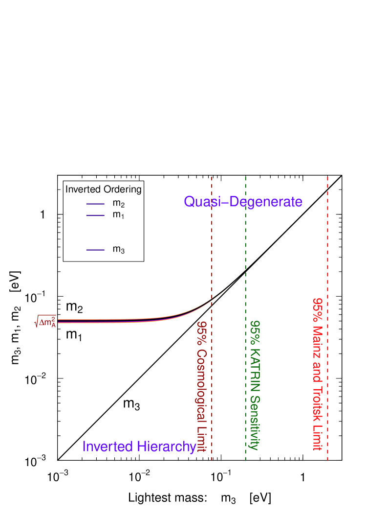
Figure 3: Values of the neutrino masses as functions of the lightest mass in the two possible cases of normal ordering 3 and inverted ordering 3. They have been obtained using the squared-mass differences in Tab. 2.

The matter effect is especially important for solar neutrinos, which are created as electron neutrinos by thermonuclear reactions in the center of the Sun, where the electron number density $N_{e}$ is of the order of $10^{2}\,N_{\text{A}}\,\text{cm}^{-3}$, and propagate out of the Sun through an electron density which decreases approximately in an exponential way (see Giunti and Kim [234]). In a first approximation which neglects the small effects due to $\vartheta_{13}$, $\nu_{e}$ is mixed only with $\nu_{1}$ and $\nu_{2}$, which are almost equally mixed with $\nu_{\mu}$ and $\nu_{\tau}$ (see Subsection II.5). In this approximation, the oscillations of solar neutrinos are well described by the two-neutrino $\nu_{e}$–$\nu_{a}$ mixing formalism with $\vartheta=\vartheta_{12}$. The oscillations are generated by the solar squared-mass difference

$$\Delta{m}^{2}_{\text{S}}\approx 8\times 10^{-5}\,\text{eV}^{2},$$ (58)

and

$$|\nu_{a}\rangle\simeq\hbox{} \hbox{}\cos\vartheta_{23}\,|\nu_{\mu}\rangle-\sin\vartheta_{23}\,|\nu_{\tau}\rangle$$

$$\approx\hbox{} \hbox{}(|\nu_{\mu}\rangle-|\nu_{\tau}\rangle)/\sqrt{2}.$$ (59)

An electron neutrino created in the center of the Sun is the linear combination of effective massive neutrinos

$$|\nu_{e}^{0}\rangle=\cos\vartheta_{\text{M}}^{0}|\nu^{0}_{1}\rangle+\sin\vartheta_{\text{M}}^{0}|\nu^{0}_{2}\rangle,$$ (60)

where $\nu^{0}_{1}$ and $\nu^{0}_{2}$ are the effective massive neutrinos at the point of neutrino production near the center of the Sun and $\vartheta_{\text{M}}^{0}$ is the corresponding effective mixing angle. Since the resonance is crossed adiabatically, there are no transitions between the effective massive neutrinos during propagation and the state which emerges from the Sun is

$$|\nu_{\text{S}}\rangle=\cos\vartheta_{\text{M}}^{0}|\nu_{1}\rangle+\sin\vartheta_{\text{M}}^{0}|\nu_{2}\rangle,$$ (61)

where $\nu_{1}$ and $\nu_{2}$ are the massive neutrinos in vacuum. Since the two massive neutrinos lose coherence during the long propagation from the Sun to the Earth [171], experiments on Earth measure the average electron neutrino survival probability [410]

$$\overline{P}_{\nu_{e}\to\nu_{e}}^{\text{S},2\nu}=\hbox{} \hbox{}\cos^{2}\vartheta_{\text{M}}^{0}|\langle\nu_{e}|\nu_{1}\rangle|^{2}+\sin^{2}\vartheta_{\text{M}}^{0}|\langle\nu_{e}|\nu_{2}\rangle|^{2}$$

$$=\hbox{} \hbox{}\frac{1}{2}+\frac{1}{2}\cos 2\vartheta_{\text{M}}^{0}\cos 2\vartheta_{12}.$$ (62)

This is a surprisingly simple expression, which depends only on the mixing angle in vacuum $\vartheta_{12}$ and on the effective mixing angle in the center of the Sun $\vartheta_{\text{M}}^{0}$, which can be easily calculated using Eq. (54). Notice that $\vartheta_{\text{M}}^{0}$ depends on the neutrino energy. With the value of $\Delta{m}^{2}_{\text{S}}$ in Eq. (58), $\vartheta_{\text{M}}^{0}\simeq\vartheta_{12}$ for $E_{\nu}\lesssim 1\,\text{MeV}$ and $\vartheta_{\text{M}}^{0}\simeq\pi/2$ for $E_{\nu}\gtrsim 5\,\text{MeV}$ (see Giunti and Kim [234]). Therefore,

$$\overline{P}_{\nu_{e}\to\nu_{e}}^{\text{S},2\nu}\simeq\left\{\begin{array}[]{lll}\displaystyle 1-0.5\sin^{2}2\vartheta_{12}&\quad\text{for}&E_{\nu}\lesssim 1\,\text{MeV},\\ \displaystyle\sin^{2}\vartheta_{12}&\quad\text{for}&E_{\nu}\gtrsim 5\,\text{MeV}.\end{array}\right.$$ (63)

II.5 Status of three-neutrino mixing

The results of several solar, atmospheric and long-baseline neutrino oscillation experiments have proved that neutrinos are massive and mixed particles (see Giunti and Kim [234], Bilenky [104], Xing and Zhou [524], Gonzalez-Garcia et al. [245], Bellini et al. [90], Gonzalez-Garcia et al. [246], Capozzi et al. [128]). There are two groups of experiments which measured two types of flavor transition generated by two independent squared-mass differences ($\Delta{m}^{2}$): the solar squared-mass difference in Eq. (58) and the atmospheric squared-mass difference

$$\Delta{m}^{2}_{\text{A}}\approx 2\times 10^{-3}\,\text{eV}^{2}.$$ (64)

Since in the framework of three-neutrino mixing described in Subsection II.3 there are just two independent squared-mass differences, solar, atmospheric and long-baseline data have led us to the current three-neutrino mixing paradigm, with the standard assignments

$$\Delta{m}^{2}_{\text{S}}=\Delta{m}^{2}_{21}\ll\Delta{m}^{2}_{\text{A}}=\frac{1}{2}\left|\Delta{m}^{2}_{31}+\Delta{m}^{2}_{32}\right|.$$ (65)

The absolute value in the definition of $\Delta{m}^{2}_{\text{A}}$ is necessary, because there are the two possible orderings of the neutrino masses illustrated schematically in the insets of the two corresponding panels in Fig. 3: the normal ordering (NO) with $m_{1}<m_{2}<m_{3}$ and $\Delta{m}^{2}_{13},\,\Delta{m}^{2}_{23}>0$; the inverted ordering (IO) with $m_{3}<m_{1}<m_{2}$ and $\Delta{m}^{2}_{13},\,\Delta{m}^{2}_{23}<0$.

The three-neutrino mixing parameters can be determined with good precision with a global fit of neutrino oscillation data. In Tab. 2 we report the results of the latest global fit presented in Capozzi et al. [128], which agree, within the uncertainties, with the NuFIT-v1.2 [246] update of the global analysis presented in Gonzalez-Garcia et al. [245]. One can see that all the oscillation parameters are determined with precision between about 3% and 10%. The largest uncertainty is that of $\vartheta_{23}$, which is known to be close to maximal ($\pi/4$), but it is not known if it is smaller or larger than $\pi/4$. For the Dirac CP-violating phase $\delta$, there is an indication in favor of $\delta\approx 3\pi/2$, which would give maximal CP violation, but at $3\sigma$ all the values of $\delta$ are allowed, including the CP-conserving values $\delta=0,\pi$.

An open problem in the framework of three-neutrino mixing is the determination of the absolute scale of neutrino masses, which cannot be determined with neutrino oscillation experiments, because oscillations depend only on the differences of neutrino masses. However, the measurement in neutrino oscillation experiments of the neutrino squared-mass differences allows us to constrain the allowed patterns of neutrino masses. A convenient way to see the allowed patterns of neutrino masses is to plot the values of the masses as functions of the unknown lightest mass, which is $m_{1}$ in the normal ordering and $m_{3}$ in the inverted ordering, as shown in Figs. 3. We used the squared-mass differences in Tab. 2. Figure 3 shows that there are three extreme possibilities:

Parameter	Ordering	Best fit	$1\sigma$ range	$2\sigma$ range	$3\sigma$ range	rel. unc.
$\Delta{m}^{2}_{\text{S}}/10^{-5}\,\text{eV}^{2}$		7.54	7.32 – 7.80	7.15 – 8.00	6.99 – 8.18	3%
$\sin^{2}\vartheta_{12}/10^{-1}$		3.08	2.91 – 3.25	2.75 – 3.42	2.59 – 3.59	5%
$\Delta{m}^{2}_{\text{A}}/10^{-3}\,\text{eV}^{2}$	NO	2.43	2.37 – 2.49	2.30 – 2.55	2.23 – 2.61	3%
	IO	2.38	2.32 – 2.44	2.25 – 2.50	2.19 – 2.56	3%
$\sin^{2}\vartheta_{23}/10^{-1}$	NO	4.37	4.14 – 4.70	3.93 – 5.52	3.74 – 6.26	10%
	IO	4.55	4.24 – 5.94	4.00 – 6.20	3.80 – 6.41	10%
$\sin^{2}\vartheta_{13}/10^{-2}$	NO	2.34	2.15 – 2.54	1.95 – 2.74	1.76 – 2.95	8%
	IO	2.40	2.18 – 2.59	1.98 – 2.79	1.78 – 2.98	8%

Table 2: Values of the neutrino mixing parameters obtained with a global analysis of neutrino oscillation data presented in Capozzi et al. [128] in the framework of three-neutrino mixing with the normal ordering (NO) and the inverted ordering (IO). The relative uncertainty (rel. unc.) has been obtained from the $3\sigma$ range divided by 6.

A normal hierarchy

$m_{1}\ll m_{2}\ll m_{3}$. In this case

$$\hbox{}m_{2}\simeq\sqrt{\Delta{m}^{2}_{\text{S}}}\approx 9\times 10^{-3}\,\text{eV},$$ (66)

$$\hbox{}m_{3}\simeq\sqrt{\Delta{m}^{2}_{\text{A}}}\approx 5\times 10^{-2}\,\text{eV}.$$ (67)

An inverted hierarchy

$m_{3}\ll m_{1}\lesssim m_{2}$ In this case

$$m_{1}\lesssim m_{2}\simeq\sqrt{\Delta{m}^{2}_{\text{A}}}\approx 5\times 10^{-2}\,\text{eV}.$$ (68)

Quasi-degenerate masses

$m_{1}\lesssim m_{2}\lesssim m_{3}\simeq m_{\nu}$ in the normal scheme and $m_{3}\lesssim m_{1}\lesssim m_{2}\simeq m_{\nu}$ in the inverted scheme, with

$$m_{\nu}\gg\sqrt{\Delta{m}^{2}_{\text{A}}}\approx 5\times 10^{-2}\,\text{eV}.$$ (69)

There are three main sources of information on the absolute scale of neutrino masses:

Beta decay

The most robust information on neutrino masses can be obtained in $\beta$-decay experiments which measure the kinematical effect of neutrino masses on the energy spectrum of the emitted electron. Tritium $\beta$-decay experiments obtained the most stringent bounds on the neutrino masses by limiting the effective electron neutrino mass $m_{\beta}$ given by (see Giunti and Kim [234], Bilenky [104], Xing and Zhou [524])

$$m_{\beta}^{2}=\sum_{k=1}^{3}|U_{ek}|^{2}m^{2}_{k}.$$ (70)

The most stringent 95% CL limits obtained in the Mainz [318] and Troitsk [45] experiments,

$$\hbox{}m_{\beta}\leq 2.3\,\text{eV}\quad(\text{Mainz}),$$ (71)

$$\hbox{}m_{\beta}\leq 2.1\,\text{eV}\quad(\text{Troitsk}),$$ (72)

are shown in Fig. 3. The KATRIN experiment [214], which is scheduled to start data taking in 2016, is expected to have a sensitivity to $m_{\beta}$ of about 0.2 eV (also shown in Fig. 3).

Neutrinoless double-beta decay

This process occurs only if massive neutrinos are Majorana fermions and depends on the effective Majorana mass (see Giunti and Kim [234], Bilenky [104], Xing and Zhou [524], Bilenky and Giunti [105])

$$m_{\beta\beta}=\left|\sum_{k=1}^{3}U^{2}_{ek}m_{k}\right|.$$ (73)

The most stringent 90%CL limits, have been obtained combining the results of EXO [48] and KamLAND-Zen [225] experiments with ${}^{136}\text{Xe}$,

$$m_{\beta\beta}\lesssim 0.12-0.25\,\text{eV}\,\text{[\cite[citet]{\@@bibref{Authors Phrase1NumberPhrase2}{Gando:2012zm}{\@@citephrase{[}}{\@@citephrase{]}}}]},$$ (74)

and combining the results of Heidelberg-Moscow [305], IGEX [2] and GERDA [12] with ${}^{76}\text{Ge}$,

$$m_{\beta\beta}\lesssim 0.2-0.4\,\text{eV}\,\text{[\cite[citet]{\@@bibref{Authors Phrase1NumberPhrase2}{Agostini:2013mzu}{\@@citephrase{[}}{\@@citephrase{]}}}]}.$$ (75)

The intervals are caused by nuclear physics uncertainties (see Vergados et al. [505]).

Cosmology

Since light massive neutrinos are hot dark matter, cosmological data give information on the sum of neutrino masses (see Giunti and Kim [234], Bilenky [104], Xing and Zhou [524], Lesgourgues et al. [341]). The analysis of cosmological data in the framework of the standard Cold Dark Matter model with a cosmological constant ($\Lambda$CDM) disfavors neutrino masses larger than some fraction of eV, but the value of the upper bound on the sum of neutrino masses depends on model assumptions and on the considered data set (see Wong [523]). Figure 3 shows the 95% limit

$$\sum_{k=1}^{3}m_{k}<0.32\,\text{eV},$$ (76)

obtained recently by the Planck collaboration [11]. See Archidiacono et al. [37], Abazajian et al. [6], Lesgourgues and Pastor [342] for recent reviews of the implications of cosmological data for neutrino physics.

II.6 Sterile neutrinos

In the previous Subsections we have considered the standard framework of three-neutrino mixing which can explain the numerous existing measurements of neutrino oscillations as explained in Subsection II.5. However, it is possible that there are additional massive neutrinos, such as those at the eV scale suggested by anomalies found in short-baseline oscillation experiments (see Aguilar et al. [13], Abdurashitov et al. [8], Giunti and Laveder [236], Mention et al. [374], Kopp et al. [310], Conrad et al. [148], Giunti et al. [237], Kopp et al. [309], Giunti et al. [238]) or those at the keV scale, which could constitute warm dark matter according to the Neutrino Minimal Standard Model ($\nu$MSM) [40, 44, 41, 42, 43] (see also the reviews in Boyarsky et al. [120], Kusenko [320], Drewes [182], Boyarsky et al. [118]). In the flavor basis, which describes the interacting neutrino states, the additional neutrinos are sterile, because we know from the measurement of the invisible width of the $Z$ boson in the LEP experiments that the number of light active neutrinos is three [457], and the existence of a heavy fourth generation of active fermions with an active neutrino heavier than $m_{Z}/2$ is disfavored by the experimental data [517, 340]. From the theoretical point of view, it is likely that if there are sterile neutrinos, all neutrinos are Majorana particles, but the Dirac case is not excluded.

Let us consider the general case of $N_{s}$ sterile neutrinos $\nu_{s_{1}},\ldots,\nu_{s_{N_{s}}}$. In the mass basis there are $N=3+N_{s}$ massive neutrino fields $\nu_{1},\ldots,\nu_{N}$ and the mixing of the left-handed neutrino fields is given by

$$\nu_{\ell L}=\sum_{k=1}^{N}U_{\ell k}\nu_{kL}\quad(\ell=e,\mu,\tau,s_{1},\ldots,s_{N_{s}}),$$ (77)

where $U$ is a $N{\times}N$ unitary mixing matrix. The three massive neutrinos $\nu_{1}$, $\nu_{2}$, $\nu_{3}$ coincide with those in the standard three-neutrino mixing framework discussed in Subsection II.3, and $\nu_{4},\ldots,\nu_{N}$ are the additional nonstandard $N_{s}$ massive neutrinos. In order to preserve approximately the three-neutrino mixing explanation of oscillation data described in Subsection II.5, the mixing of the three active neutrinos $\nu_{e}$, $\nu_{\mu}$, $\nu_{\tau}$ with the nonstandard massive neutrinos $\nu_{4},\ldots,\nu_{N}$ must be very small:

$$|U_{\ell k}|\ll 1\quad\text{for}\quad\ell=e,\mu,\tau\quad\text{and}\quad k\geq 4,$$ (78)

which implies that

$$|U_{s_{n}k}|\ll 1\quad\text{for}\quad n=1,\ldots,N_{s}\quad\text{and}\quad k\leq 3.$$ (79)

Since the mixing in the sterile sector is arbitrary, it is convenient to choose

$$U_{s_{n}k}=0\quad\text{for}\quad n\neq k-3\quad\text{and}\quad k\geq 4.$$ (80)

Then, from Eq. (79) we have

$$1-|U_{s_{k-3}k}|^{2}\ll 1,\quad\text{for}\quad k\geq 4.$$ (81)

The numerical values of the inequalities (78)–(81) depend on the model and on the experimental data under consideration. In this review we consider only these generic inequalities in order to present general results on the neutrino dipole moments in Subsections IV.1 and IV.2 and on neutrino radiative decay in Subsection V.1.

III Electromagnetic form factors

The importance of neutrino electromagnetic properties was first mentioned by Pauli in 1930, when he postulated the existence of this particle and discussed the possibility that the neutrino might have a magnetic moment [412]. Systematic theoretical studies of neutrino electromagnetic properties started after it was shown that in the extended Standard Model with right-handed neutrinos the magnetic moment of a massive neutrino is, in general, nonvanishing and that its value is determined by the neutrino mass [362, 332, 217, 414, 408, 469, 107].

Neutrino electromagnetic properties are important because they are directly connected to fundamentals of particle physics. For example, neutrino electromagnetic properties can be used to distinguish Dirac and Majorana neutrinos, because Dirac neutrinos can have both diagonal and off-diagonal magnetic and electric dipole moments, whereas only the off-diagonal ones are allowed for Majorana neutrinos (see Schechter and Valle [458], Shrock [469], Pal and Wolfenstein [408], Nieves [390], Kayser [297, 298]). This is shown in details in the following Subsections. Another important case in which Dirac and Majorana neutrinos have quite different observable effects is the spin-flavor precession in an external magnetic field discussed in Subsection VI.2. Neutrino electromagnetic properties are also probes of new physics beyond the Standard Model, because in the Standard Model neutrinos can have only a charge radius (see Subsection III.3 and Subsection VII.2). The discovery of other neutrino electromagnetic properties would be a signal of new physics beyond the Standard Model (see Bell et al. [88, 87], Bell [86], Novales-Sanchez et al. [397]).

In this Section we discuss the general form of the electromagnetic interactions of Dirac and Majorana neutrinos in the one-photon approximation. In Subsection III.1 we derive the general expression of the effective electromagnetic coupling of Dirac neutrinos in terms of electromagnetic form factors and we discuss the properties of the form factors under CP and CPT transformations. In Subsection III.2 we consider Majorana neutrinos and in Subsection III.3 we consider the Standard Model case of massless Weyl neutrinos.

III.1 Dirac neutrinos

Figure 4: Tree-level coupling of a charged fermion $\mathfrak{f}$ with a photon $\gamma$ 4 and effective one-photon coupling of a neutrino with a photon 4.

In the Standard Model, the interaction of a fermionic field $\mathfrak{f}(x)$ with the electromagnetic field $A^{\mu}(x)$ is given by the interaction Hamiltonian

$$\mathcal{H}_{\text{em}}^{(\mathfrak{f})}(x)=j_{\mu}^{(\mathfrak{f})}(x)A^{\mu}(x)=\mathbbm{q}_{\mathfrak{f}}\overline{\mathfrak{f}}(x)\gamma_{\mu}\mathfrak{f}(x)A^{\mu}(x),$$ (82)

where $\mathbbm{q}_{\mathfrak{f}}$ is the charge of the fermion $\mathfrak{f}$. Figure 4 shows the corresponding tree-level Feynman diagram (the photon $\gamma$ is the quantum of the electromagnetic field $A^{\mu}(x)$).

For neutrinos the electric charge is zero and there are no electromagnetic interactions at tree-level. However, such interactions can arise at the quantum level from loop diagrams at higher order of the perturbative expansion of the interaction. In the one-photon approximation, the electromagnetic interactions of a neutrino field $\nu(x)$ can be described by the effective interaction Hamiltonian

$$\mathcal{H}_{\text{em}}^{(\nu)}(x)=j_{\mu}^{(\nu)}(x)A^{\mu}(x)=\overline{\nu}(x)\Lambda_{\mu}\nu(x)A^{\mu}(x),$$ (83)

where, $j_{\mu}^{(\nu)}(x)$ is the neutrino effective electromagnetic current four-vector and $\Lambda_{\mu}$ is a $4\times 4$ matrix in spinor space which can contain space-time derivatives, such that $j_{\mu}^{(\nu)}(x)$ transforms as a four-vector. Since radiative corrections are generated by weak interactions which are not invariant under a parity transformation, $j_{\mu}^{(\nu)}(x)$ can be a sum of polar and axial parts. The corresponding diagram for the interaction of a neutrino with a photon is shown in Fig. 4, where the blob represents the quantum loop contributions.

As we will see in the following, the neutrino electromagnetic properties corresponding to the diagram in Fig. 4 include charge and magnetic form factors. Let us emphasize that these neutrino electromagnetic properties can exist even if neutrinos are elementary particles, without an internal structure, because they are generated by quantum loop effects. Thus, the neutrino charge and magnetic form factors have a different origin from the neutron charge and magnetic form factors (also called Dirac and Pauli form factors), which are mainly due to its internal quark structure. For example, the neutrino magnetic moment (which is the magnetic form factor for interactions with real photons, i.e. $q^{2}=0$ in Fig. 4) have the same quantum origin as the anomalous magnetic moment of the electron (see Greiner and Reinhardt [258]).

We are interested in the neutrino part of the amplitude corresponding to the diagram in Fig. 4, which is given by the matrix element

$$\langle\nu(p_{f},h_{f})|j_{\mu}^{(\nu)}(x)|\nu(p_{i},h_{i})\rangle,$$ (84)

where $p_{i}$ ($p_{f}$) and $h_{i}$ ($h_{f}$) are the four-momentum and helicity of the initial (final) neutrino. Taking into account that

$$\partial^{\mu}j_{\mu}^{(\nu)}(x)=i\left[\mathcal{P}^{\mu},j_{\mu}^{(\nu)}(x)\right],$$ (85)

where $\mathcal{P}^{\mu}$ is the four-momentum operator which generate translations, the effective current can be written as

$$j_{\mu}^{(\nu)}(x)=e^{i\mathcal{P}\cdot x}j_{\mu}^{(\nu)}(0)e^{-i\mathcal{P}\cdot x}.$$ (86)

Since $\mathcal{P}^{\mu}|\nu(p)\rangle=p^{\mu}|\nu(p)\rangle$, we have

$$\langle\nu(p_{f})|j_{\mu}^{(\nu)}(x)|\nu(p_{i})\rangle=e^{i(p_{f}-p_{i})\cdot x}\langle\nu(p_{f})|j_{\mu}^{(\nu)}(0)|\nu(p_{i})\rangle,$$ (87)

where we suppressed for simplicity the helicity labels which are not of immediate relevance. Here we see that the unknown quantity which determines the neutrino-photon interaction is $\langle\nu(p_{f})|j_{\mu}^{(\nu)}(0)|\nu(p_{i})\rangle$. Considering that the incoming and outgoing neutrinos are free particles which are described by free Dirac fields with the Fourier expansion in Eq. (548), we have

$$\langle\nu(p_{f})|j_{\mu}^{(\nu)}(0)|\nu(p_{i})\rangle=\overline{u}(p_{f})\Lambda_{\mu}(p_{f},p_{i})u(p_{i}).$$ (88)

The electromagnetic properties of neutrinos are embodied by the vertex function $\Lambda_{\mu}(p_{f},p_{i})$, which is a matrix in spinor space and can be decomposed in terms of linearly independent products of Dirac $\gamma$ matrices and the available kinematical four-vectors $p_{i}$ and $p_{f}$. As shown in Appendix B, the most general decomposition can be written as

$$\hbox{}\Lambda_{\mu}(p_{f},p_{i})=\mathbbm{f}_{1}(q^{2})q_{\mu}+\mathbbm{f}_{2}(q^{2})q_{\mu}\gamma_{5}+\mathbbm{f}_{3}(q^{2})\gamma_{\mu}$$

$$\hbox{}+\mathbbm{f}_{4}(q^{2})\gamma_{\mu}\gamma_{5}+\mathbbm{f}_{5}(q^{2})\sigma_{\mu\nu}q^{\nu}+\mathbbm{f}_{6}(q^{2})\epsilon_{\mu\nu\rho\gamma}q^{\nu}\sigma^{\rho\gamma},$$ (89)

where $\mathbbm{f}_{k}(q^{2})$ are six Lorentz-invariant form factors ($k=1,\ldots,6$) and $q$ is the four-momentum of the photon, which is given by

$$q=p_{i}-p_{f},$$ (90)

from energy-momentum conservation. Notice that the form factors depend only on $q^{2}$, which is the only available Lorentz-invariant kinematical quantity, since $(p_{i}+p_{f})^{2}=4m^{2}-q^{2}$. Therefore, $\Lambda_{\mu}(p_{f},p_{i})$ depends only on $q$ and from now on we will denote it as $\Lambda_{\mu}(q)$.

Since the Hamiltonian and the electromagnetic field are Hermitian ($\mathcal{H}_{\text{em}}^{(\nu)\dagger}=\mathcal{H}_{\text{em}}^{(\nu)}$ and $A^{\mu\dagger}=A^{\mu}$), the effective current must be Hermitian, $j_{\mu}^{(\nu)\dagger}=j_{\mu}^{(\nu)}$. Hence, we have

$$\langle\nu(p_{f})|j_{\mu}^{(\nu)}(0)|\nu(p_{i})\rangle=\langle\nu(p_{i})|j_{\mu}^{(\nu)}(0)|\nu(p_{f})\rangle^{*},$$ (91)

which leads to

$$\Lambda_{\mu}(q)=\gamma^{0}\Lambda_{\mu}^{\dagger}(-q)\gamma^{0}.$$ (92)

Using the properties of the Dirac matrices (see Appendix A), one can find that this constraint implies that

$$\mathbbm{f}_{2},\quad\mathbbm{f}_{3},\quad\mathbbm{f}_{4}\quad\text{are real},$$ (93)

and

$$\mathbbm{f}_{1},\quad\mathbbm{f}_{5},\quad\mathbbm{f}_{6}\quad\text{are imaginary}.$$ (94)

The number of independent form factors can be reduced by imposing current conservation, $\partial^{\mu}j_{\mu}^{(\nu)}(x)=0$, which is required by gauge invariance (i.e. invariance of $\mathcal{H}_{\text{em}}^{(\nu)}(x)$ under the transformation $A^{\mu}(x)\to A^{\mu}(x)+\partial^{\mu}\varphi(x)$ for any $\varphi(x)$, which leaves invariant the electromagnetic tensor $F^{\mu\nu}=\partial^{\mu}A^{\nu}-\partial^{\nu}A^{\mu}$). Using Eq. (85), current conservation implies that

$$\langle\nu(p_{f})|\left[\mathcal{P}^{\mu},j_{\mu}^{(\nu)}(0)\right]|\nu(p_{i})\rangle=0.$$ (95)

Hence, in momentum space we have the constraint

$$q^{\mu}\,\overline{u}(p_{f})\Lambda_{\mu}(q)u(p_{i})=0,$$ (96)

which implies that

$$\mathbbm{f}_{1}(q^{2})q^{2}+\mathbbm{f}_{2}(q^{2})q^{2}\gamma_{5}+2m\mathbbm{f}_{4}(q^{2})\gamma_{5}=0.$$ (97)

Since $\gamma_{5}$ and the unity matrix are linearly independent, we obtain the constraints

$$\mathbbm{f}_{1}(q^{2})=0,\quad\mathbbm{f}_{4}(q^{2})=-\mathbbm{f}_{2}(q^{2})q^{2}/2m.$$ (98)

Therefore, in the most general case consistent with Lorentz and electromagnetic gauge invariance, the vertex function $\Lambda_{\mu}(q)$ is defined in terms of four form factors [390, 297, 298],

$$\Lambda_{\mu}(q)=\hbox{} \hbox{}\mathbbm{f}_{Q}(q^{2})\gamma_{\mu}-\mathbbm{f}_{M}(q^{2})i\sigma_{\mu\nu}q^{\nu}+\mathbbm{f}_{E}(q^{2})\sigma_{\mu\nu}q^{\nu}\gamma_{5}$$

$$\hbox{}+\mathbbm{f}_{A}(q^{2})(q^{2}\gamma_{\mu}-q_{\mu}\not{q})\gamma_{5},$$ (99)

where $\mathbbm{f}_{Q}=\mathbbm{f}_{3}$, $\mathbbm{f}_{M}=i\mathbbm{f}_{5}$, $\mathbbm{f}_{E}=-2i\mathbbm{f}_{6}$ and $\mathbbm{f}_{A}=-\mathbbm{f}_{2}/2m$ are the real charge, dipole magnetic and electric, and anapole neutrino form factors. The term involving the electric form factor corresponds to the last term in Eq. (89), in which we took into account the identity in Eq. (519). In the term involving the anapole form factor we used the identity $\overline{u}(p_{f})\not{q}\gamma^{5}u(p_{i})=2m\,\overline{u}(p_{f})\gamma^{5}u(p_{i})$, which is easily obtained from Eqs. (510) and (535).

The physical meaning of the dipole magnetic and electric neutrino form factors is discussed in Section IV and that of the charge and anapole in Section VII. Here we only remark that for the coupling with a real photon ($q^{2}=0$)

$$\mathbbm{f}_{Q}(0)=\mathbbm{q},\quad\mathbbm{f}_{M}(0)=\bbmu,\quad\mathbbm{f}_{E}(0)=\bbespilon,\quad\mathbbm{f}_{A}(0)=\mathbbm{a},$$ (100)

where $\mathbbm{q}$, $\bbmu$, $\bbespilon$ and $\mathbbm{a}$ are, respectively, the neutrino charge, magnetic moment, electric moment and anapole moment. Although above we stated that $\mathbbm{q}=0$, here we did not enforce this equality because in some theories beyond the Standard Model neutrinos can be millicharged particles, as explained in Subsection VII.1.

Now it is interesting to study the properties of $\mathcal{H}_{\text{em}}^{(\nu)}(x)$ under a CP transformation, in order to find which of the terms in Eq. (99) violate CP. The reason is that, whereas it is well known that weak interactions violate maximally C and P, the violation of CP is a more exotic phenomenon, which has been observed so far only in the hadron sector (see Bilenky [106]).

Using the transformation (559) of a fermion field under an active CP transformation one can find that for the Standard Model electric current $j_{\mu}(x)$ in Eq. (82) we have

$$j_{\mu}(x)\xrightarrow{\;\text{CP}\;}\mathsf{U}_{\text{CP}}j_{\mu}(x)\mathsf{U}_{\text{CP}}^{\dagger}=-j^{\mu}(x_{\text{P}}).$$ (101)

Hence, the Standard Model electromagnetic interaction Hamiltonian $\mathcal{H}_{\text{em}}^{(\nu)}(x)$ is left invariant by

$$A_{\mu}(x)\xrightarrow{\;\text{CP}\;}-A^{\mu}(x_{\text{P}}).$$ (102)

CP is conserved in neutrino electromagnetic interactions (in the one-photon approximation) if $j_{\mu}^{(\nu)}(x)$ transforms as $j_{\mu}(x)$:

$$\text{CP}\quad\Longleftrightarrow\quad\mathsf{U}_{\text{CP}}j_{\mu}^{(\nu)}(x)\mathsf{U}_{\text{CP}}^{\dagger}=-j^{\mu}_{(\nu)}(x_{\text{P}}).$$ (103)

For the matrix element (88) we obtain

$$\text{CP}\quad\Longleftrightarrow\quad\Lambda_{\mu}(q)\xrightarrow{\;\text{CP}\;}-\Lambda^{\mu}(q).$$ (104)

Using the formulae in Appendix A, one can find that under a CP transformation we have

$$\Lambda_{\mu}(q)\xrightarrow{\;\text{CP}\;}\gamma^{0}\mathcal{C}\Lambda_{\mu}^{T}(q_{\text{P}})\mathcal{C}^{\dagger}\gamma^{0},$$ (105)

with $q^{\mu}_{\text{P}}=q_{\mu}$. Using the form-factor expansion in Eq. (99), we obtain

$$\hbox{}\Lambda_{\mu}(q)\xrightarrow{\;\text{CP}\;}-\big{[}\mathbbm{f}_{Q}(q^{2})\gamma^{\mu}-\mathbbm{f}_{M}(q^{2})i\sigma^{\mu\nu}q_{\nu}$$

$$\hbox{}-\mathbbm{f}_{E}(q^{2})\sigma^{\mu\nu}q_{\nu}\gamma_{5}+\mathbbm{f}_{A}(q^{2})(q^{2}\gamma^{\mu}-q^{\mu}\not{q})\gamma_{5}\big{]}.$$ (106)

Therefore, only the electric dipole form factor violates CP:

$$\text{CP}\quad\Longleftrightarrow\quad\mathbbm{f}_{E}(q^{2})=0.$$ (107)

Figure 5: Effective one-photon coupling of neutrinos with the electromagnetic field, taking into account possible transitions between two different initial and final massive neutrinos $\nu_{i}$ and $\nu_{f}$.

So far, in this Section we have considered only one massive neutrino field $\nu(x)$, but from the discussion of neutrino mixing in Section II we know that there are at least three massive neutrino fields in nature. Therefore, we must generalize the discussion to the case of $N$ massive neutrino fields $\nu_{k}(x)$ with respective masses $m_{k}$ ($k=1,\ldots,N$). The effective electromagnetic interaction Hamiltonian in Eq. (83) is generalized to

$$\mathcal{H}_{\text{em}}^{(\nu)}(x)=j_{\mu}^{(\nu)}(x)A^{\mu}(x)=\sum_{k,j=1}^{N}\overline{\nu_{k}}(x)\Lambda^{kj}_{\mu}\nu_{j}(x)A^{\mu}(x),$$ (108)

where we take into account possible transitions between different massive neutrinos. The physical effect of $\mathcal{H}_{\text{em}}^{(\nu)}$ is described by the effective electromagnetic vertex in Fig. 5, with the neutrino matrix element

$$\langle\nu_{f}(p_{f})|j_{\mu}^{(\nu)}(0)|\nu_{i}(p_{i})\rangle=\overline{u_{f}}(p_{f})\Lambda^{fi}_{\mu}(p_{f},p_{i})u_{i}(p_{i}).$$ (109)

As in the case of one massive neutrino field (see Appendix B), $\Lambda^{fi}_{\mu}(p_{f},p_{i})$ depends only on the four-momentum $q$ transferred to the photon and can be expressed in terms of six Lorentz-invariant form factors:

$$\hbox{}\Lambda^{fi}_{\mu}(q)=\mathbbm{f}_{1}^{fi}(q^{2})q_{\mu}+\mathbbm{f}_{2}^{fi}(q^{2})q_{\mu}\gamma_{5}+\mathbbm{f}_{3}^{fi}(q^{2})\gamma_{\mu}$$

$$\hbox{}+\mathbbm{f}_{4}^{fi}(q^{2})\gamma_{\mu}\gamma_{5}+\mathbbm{f}_{5}^{fi}(q^{2})\sigma_{\mu\nu}q^{\nu}+\mathbbm{f}_{6}^{fi}(q^{2})\epsilon_{\mu\nu\rho\gamma}q^{\nu}\sigma^{\rho\gamma}.$$ (110)

The Hermitian nature of $j_{\mu}^{(\nu)}$ implies that $\langle\nu_{f}(p_{f})|j_{\mu}^{(\nu)}(0)|\nu_{i}(p_{i})\rangle=\langle\nu_{i}(p_{i})|j_{\mu}^{(\nu)}(0)|\nu_{f}(p_{f})\rangle^{*}$, leading to the constraint

$$\Lambda^{fi}_{\mu}(q)=\gamma^{0}[\Lambda^{if}_{\mu}(-q)]^{\dagger}\gamma^{0}.$$ (111)

Considering the $N{\times}N$ form-factor matrices $\mathbbm{f}_{k}$ in the space of massive neutrinos with components $\mathbbm{f}_{k}^{fi}$ for $k=1,\ldots,6$, we find that

$$\mathbbm{f}_{2},\quad\mathbbm{f}_{3},\quad\mathbbm{f}_{4}\quad\text{are Hermitian},$$ (112)

and

$$\mathbbm{f}_{1},\quad\mathbbm{f}_{5},\quad\mathbbm{f}_{6}\quad\text{are antihermitian}.$$ (113)

Following the same method used in Eqs. (85)–(97), one can find that current conservation implies the constraints

$$\hbox{}\mathbbm{f}_{1}^{fi}(q^{2})q^{2}+\mathbbm{f}_{3}^{fi}(q^{2})(m_{f}-m_{i})=0,$$ (114)

$$\hbox{}\mathbbm{f}_{2}^{fi}(q^{2})q^{2}+\mathbbm{f}_{4}^{fi}(q^{2})(m_{f}+m_{i})=0.$$ (115)

Therefore, we obtain

$$\Lambda^{fi}_{\mu}(q)=\hbox{} \hbox{}\left(\gamma_{\mu}-q_{\mu}\not{q}/q^{2}\right)\left[\mathbbm{f}_{Q}^{fi}(q^{2})+\mathbbm{f}_{A}^{fi}(q^{2})q^{2}\gamma_{5}\right]$$

$$\hbox{}-i\sigma_{\mu\nu}q^{\nu}\left[\mathbbm{f}_{M}^{fi}(q^{2})+i\mathbbm{f}_{E}^{fi}(q^{2})\gamma_{5}\right],$$ (116)

where $\mathbbm{f}_{Q}^{fi}=\mathbbm{f}_{3}^{fi}$, $\mathbbm{f}_{M}^{fi}=i\mathbbm{f}_{5}^{fi}$, $\mathbbm{f}_{E}^{fi}=-2i\mathbbm{f}_{6}^{fi}$ and $\mathbbm{f}_{A}^{fi}=-\mathbbm{f}_{2}^{fi}/(m_{f}+m_{i})$, with

$$\mathbbm{f}_{\Omega}^{fi}=(\mathbbm{f}_{\Omega}^{if})^{*}\qquad(\Omega=Q,M,E,A).$$ (117)

Note that since $\overline{u_{f}}(p_{f})\not{q}u_{i}(p_{i})=(m_{f}-m_{i})\,\overline{u_{f}}(p_{f})u_{i}(p_{i})$, if $f=i$ Eq. (116) correctly reduces to Eq. (99).

The form-factors with $f=i$ are called “diagonal”, whereas those with $f{\neq}i$ are called “off-diagonal” or “transition form-factors”. This terminology follows from the expression

$$\Lambda_{\mu}(q)=\hbox{} \hbox{}\left(\gamma_{\mu}-q_{\mu}\not{q}/q^{2}\right)\left[\mathbbm{f}_{Q}(q^{2})+\mathbbm{f}_{A}(q^{2})q^{2}\gamma_{5}\right]$$

$$\hbox{}-i\sigma_{\mu\nu}q^{\nu}\left[\mathbbm{f}_{M}(q^{2})+i\mathbbm{f}_{E}(q^{2})\gamma_{5}\right],$$ (118)

in which $\Lambda_{\mu}(q)$ is a $N{\times}N$ matrix in the space of massive neutrinos expressed in terms of the four Hermitian $N{\times}N$ matrices of form factors

$$\mathbbm{f}_{\Omega}=\mathbbm{f}_{\Omega}^{\dagger}\qquad(\Omega=Q,M,E,A).$$ (119)

For the coupling with a real photon ($q^{2}=0$) we have

$$\mathbbm{f}_{Q}^{fi}(0)=\mathbbm{q}_{fi},\ \mathbbm{f}_{M}^{fi}(0)=\bbmu_{fi},\ \mathbbm{f}_{E}^{fi}(0)=\bbespilon_{fi},\ \mathbbm{f}_{A}^{fi}(0)=\mathbbm{a}_{fi},$$ (120)

where $\mathbbm{q}_{fi}$, $\bbmu_{fi}$, $\bbespilon_{fi}$ and $\mathbbm{a}_{fi}$ are, respectively, the neutrino charge, magnetic moment, electric moment and anapole moment of diagonal ($f=i$) and transition ($f{\neq}i$) types.

Considering now CP invariance, the transformation (103) of $j_{\mu}^{(\nu)}(x)$ implies the constraint in Eq. (104) for the $N{\times}N$ matrix $\Lambda_{\mu}(q)$ in the space of massive neutrinos. Using the formulae in Appendix A, we obtain

$$\Lambda_{\mu}^{fi}(q)\xrightarrow{\;\text{CP}\;}\xi^{\text{CP}}_{f}{\xi^{\text{CP}}_{i}}^{*}\gamma^{0}\mathcal{C}[\Lambda_{\mu}^{if}(q_{\text{P}})]^{T}\mathcal{C}^{\dagger}\gamma^{0},$$ (121)

where $\xi^{\text{CP}}_{k}$ is the CP phase of $\nu_{k}$. Since the massive neutrinos take part to standard charged-current weak interactions, their CP phases are equal if CP is conserved (see Giunti and Kim [234]). Hence, we have

$$\Lambda_{\mu}^{fi}(q)\xrightarrow{\;\text{CP}\;}\gamma^{0}\mathcal{C}[\Lambda_{\mu}^{if}(q_{\text{P}})]^{T}\mathcal{C}^{\dagger}\gamma^{0}.$$ (122)

Using the form-factor expansion in Eq. (116), we obtain

$$\Lambda_{\mu}^{fi}(q)\xrightarrow{\;\text{CP}\;}\hbox{} \hbox{}-\Big{\{}\left(\gamma^{\mu}-q^{\mu}\not{q}/q^{2}\right)\left[\mathbbm{f}_{Q}^{if}(q^{2})+\mathbbm{f}_{A}^{if}(q^{2})q^{2}\gamma_{5}\right]$$

$$\hbox{}-i\sigma^{\mu\nu}q_{\nu}\left[\mathbbm{f}_{M}^{if}(q^{2})-i\mathbbm{f}_{E}^{if}(q^{2})\gamma_{5}\right]\Big{\}}.$$ (123)

Imposing the constraint in Eq. (104), for the form factors we obtain

$$\text{CP}\quad\Longleftrightarrow\quad\left\{\begin{array}[]{l}\displaystyle\mathbbm{f}_{\Omega}^{fi}=\mathbbm{f}_{\Omega}^{if}=(\mathbbm{f}_{\Omega}^{fi})^{*}\qquad(\Omega=Q,M,A),\\ \displaystyle\mathbbm{f}_{E}^{fi}=-\mathbbm{f}_{E}^{if}=-(\mathbbm{f}_{E}^{fi})^{*},\end{array}\right.$$ (124)

where, in the last equalities, we took into account the constraints (117). Therefore, diagonal electric form factors violate CP, in agreement with the one-generation constraint in Eq. (107). For the Hermitian $N{\times}N$ form-factor matrices, we obtain that if CP is conserved $\mathbbm{f}_{Q}$, $\mathbbm{f}_{M}$ and $\mathbbm{f}_{A}$ are real and symmetric and $\mathbbm{f}_{E}$ is imaginary and antisymmetric:

$$\text{CP}\quad\Longleftrightarrow\quad\left\{\begin{array}[]{l}\displaystyle\mathbbm{f}_{\Omega}=\mathbbm{f}_{\Omega}^{\text{T}}=\mathbbm{f}_{\Omega}^{*}\qquad(\Omega=Q,M,A),\\ \displaystyle\mathbbm{f}_{E}=-\mathbbm{f}_{E}^{\text{T}}=-\mathbbm{f}_{E}^{*}.\end{array}\right.$$ (125)

Let us now consider antineutrinos. Using for the massive neutrino fields the Fourier expansion in Eq. (548), the effective antineutrino matrix element for $\bar{\nu}_{i}(p_{i})\to\bar{\nu}_{f}(p_{f})$ transitions is given by

$$\langle\bar{\nu}_{f}(p_{f})|j_{\mu}^{(\nu)}(0)|\bar{\nu}_{i}(p_{i})\rangle=-\overline{v_{i}}(p_{i})\Lambda^{if}_{\mu}(q)v_{f}(p_{f}).$$ (126)

Using the relation (540) we can write it as

$$\langle\bar{\nu}_{f}(p_{f})|j_{\mu}^{(\nu)}(0)|\bar{\nu}_{i}(p_{i})\rangle=\overline{u_{f}}(p_{f})\mathcal{C}[\Lambda^{if}_{\mu}(q)]^{T}\mathcal{C}^{\dagger}u_{i}(p_{i}),$$ (127)

where transposition operates in spinor space. Therefore, the effective form-factor matrix in spinor space for antineutrinos is given by

$$\overline{\Lambda}^{fi}_{\mu}(q)=\mathcal{C}[\Lambda^{if}_{\mu}(q)]^{T}\mathcal{C}^{\dagger}.$$ (128)

Using the properties of the charge-conjugation matrix, the expression (116) for $\Lambda^{if}_{\mu}(q)$, and the hermiticity in Eq. (117), we obtain the antineutrino form factors

$$\hbox{}\overline{\mathbbm{f}}_{\Omega}^{fi}=-\mathbbm{f}_{\Omega}^{if}=-(\mathbbm{f}_{\Omega}^{fi})^{*}\qquad(\Omega=Q,M,E),$$ (129)

$$\hbox{}\overline{\mathbbm{f}}_{A}^{fi}=\mathbbm{f}_{A}^{if}=(\mathbbm{f}_{A}^{fi})^{*}.$$ (130)

Therefore, in particular the diagonal magnetic and electric moments of neutrinos and antineutrinos, which are real, have the same size with opposite signs, as the charge, if it exists. On the other hand, the real diagonal neutrino and antineutrino anapole moments are equal.

It is interesting to note that the relations in Eqs. (129) and (130) between neutrino and antineutrino form factors are a consequence of CPT symmetry, which is a fundamental symmetry of local relativistic Quantum Field Theory (see Greenberg [256]). In order to prove this statement, let us first consider the CPT transformation of the Standard Model electric current $j_{\mu}(x)$ in Eq. (82): using Eq. (561) we have

$$j_{\mu}(x)\xrightarrow{\;\text{CPT}\;}\mathsf{U}_{\text{CPT}}j_{\mu}(x)\mathsf{U}_{\text{CPT}}^{\dagger}=-j_{\mu}(-x).$$ (131)

Therefore, the Standard Model electromagnetic interaction Hamiltonian $\mathcal{H}_{\text{em}}^{(\nu)}(x)$ is left invariant by

$$A_{\mu}(x)\xrightarrow{\;\text{CPT}\;}-A_{\mu}(-x).$$ (132)

CPT is conserved by the neutrino effective electromagnetic interaction Hamiltonian in Eq. (108) if $j_{\mu}^{(\nu)}(x)$ transforms as $j_{\mu}(x)$:

$$\text{CPT}\quad\Longleftrightarrow\quad\mathsf{U}_{\text{CPT}}j_{\mu}^{(\nu)}(x)\mathsf{U}_{\text{CPT}}^{\dagger}=-j_{\mu}^{(\nu)}(-x).$$ (133)

In order to find the implications of this relation for the antineutrino matrix element in Eq. (126), we need to consider it taking into account the helicities of the initial and final neutrinos, because CPT reverses helicities. Thus, assuming CPT and inserting $\mathsf{U}_{\text{CPT}}^{\dagger}\mathsf{U}_{\text{CPT}}=1$ on both sides of $j_{\mu}^{(\nu)}(0)$, we obtain

$$\hbox{}\overline{M}_{fi}=\langle\bar{\nu}_{f}(p_{f},h_{f})|j_{\mu}^{(\nu)}(0)|\bar{\nu}_{i}(p_{i},h_{i})\rangle$$

$$\hbox{}=-\langle\bar{\nu}_{f}(p_{f},h_{f})|\mathsf{U}_{\text{CPT}}^{\dagger}j_{\mu}^{(\nu)}(0)\mathsf{U}_{\text{CPT}}|\bar{\nu}_{i}(p_{i},h_{i})\rangle.$$ (134)

Now we take into account that the application of $\mathsf{U}_{\text{CPT}}$ to a neutrino state transforms it into an antineutrino state. Using the notation and conventions of Giunti and Kim [234] we have

$$\mathsf{U}_{\text{CPT}}|\bar{\nu}_{k}(p_{k},h_{k})\rangle=-\zeta(h)\,{\xi^{\text{CPT}}_{k}}^{*}|\nu_{k}(p_{k},-h_{k})\rangle,$$ (135)

where $\zeta(h)$ is a phase coming from the relation

$$\gamma^{5}\,v^{(-h)}(p)=\zeta(h)\,u^{(h)}(p),$$ (136)

and $\zeta(-h)=-\zeta(h)$. For the CPT phases $\xi^{\text{CPT}}_{k}$, we assume that they are all equal, as we have done for the CP phases in Eq. (121). Then, using Eq. (135) and taking into account the antiunitarity of $\mathsf{U}_{\text{CPT}}$, Eq. (134) becomes

$$\overline{M}_{fi}=-\zeta(h_{f})\zeta^{*}(h_{i})\langle\nu_{i}(p_{i},-h_{i})|j_{\mu}^{(\nu)}(0)|\nu_{f}(p_{f},-h_{f})\rangle.$$ (137)

This is the crucial relation between the neutrino and antineutrino matrix elements which follows from CPT invariance. Using for the neutrino matrix element the expression (109) and the relation (136), we obtain

$$\overline{M}_{fi}=\overline{v_{i}^{(h_{i})}}(p_{i})\gamma^{5}\Lambda^{if}_{\mu}(-q)\gamma^{5}v_{f}^{(h_{f})}(p_{f}).$$ (138)

Taking into account the form-factor expression of $\Lambda^{fi}_{\mu}(q)$ in Eq. (116), we have $\gamma^{5}\Lambda^{if}_{\mu}(-q)\gamma^{5}=-\Lambda^{if}_{\mu}(q)$, which leads to

$$\overline{M}_{fi}=-\overline{v_{i}^{(h_{i})}}(p_{i})\Lambda^{if}_{\mu}(q)v_{f}^{(h_{f})}(p_{f}).$$ (139)

This expression for the antineutrino matrix element coincides with Eq. (126) and implies the relations (129) and (130) for the form factors.

Thus, we obtained the expression (126) for the antineutrino matrix element in a complicated way, assuming only CPT invariance and the expression (109) for the neutrino matrix element. This result is a tautology in the theoretical framework in which we are working, because CPT is a fundamental symmetry of any local relativistic Quantum Field Theory (see Greenberg [256]). However, in some theories beyond the Standard Model small CPT violations can exist (see Tsukerman [504]), which may be revealed by finding violations of the equalities in Eqs. (129) and (130).

III.2 Majorana neutrinos

A Majorana neutrino is a neutral spin 1/2 particle which coincides with its antiparticle. The four degrees of freedom of a Dirac field (two helicities and two particle-antiparticle) are reduced to two (two helicities) by the Majorana constraint in Eq. (24). Since a Majorana field has half the degrees of freedom of a Dirac field, it is possible that its electromagnetic properties are reduced. From the relations (129) and (130) between neutrino and antineutrino form factors in the Dirac case, we can infer that in the Majorana case the charge, magnetic and electric form-factor matrices are antisymmetric and the anapole form-factor matrix is symmetric. In order to confirm this deduction, let us calculate the neutrino matrix element corresponding to the effective electromagnetic vertex in Fig. 5, with the effective interaction Hamiltonian in Eq. (108), which takes into account possible transitions between two different initial and final massive Majorana neutrinos $\nu_{i}$ and $\nu_{f}$. Using the Fourier expansion (552) for the neutrino Majorana fields we obtain

$$\langle\nu_{f}(p_{f})|j_{\mu}^{(\nu)}(0)|\nu_{i}(p_{i})\rangle\hbox{} \hbox{}=\overline{u_{f}}(p_{f})\Lambda^{fi}_{\mu}(p_{f},p_{i})u_{i}(p_{i})$$

$$\hbox{}-\overline{v_{i}}(p_{i})\Lambda^{if}_{\mu}(p_{f},p_{i})v_{f}(p_{f}).$$ (140)

Using Eq. (540), we can write it as

$$\overline{u_{f}}(p_{f})\left\{\Lambda^{fi}_{\mu}(p_{f},p_{i})+\mathcal{C}[\Lambda^{if}_{\mu}(p_{f},p_{i})]^{T}\mathcal{C}^{\dagger}\right\}u_{i}(p_{i}),$$ (141)

where transposition operates in spinor space. Therefore the effective form-factor matrix in spinor space for Majorana neutrinos is given by

$$\Lambda^{\text{M}fi}_{\mu}(p_{f},p_{i})=\Lambda^{fi}_{\mu}(p_{f},p_{i})+\mathcal{C}[\Lambda^{if}_{\mu}(p_{f},p_{i})]^{T}\mathcal{C}^{\dagger}.$$ (142)

As in the case of Dirac neutrinos, $\Lambda^{fi}_{\mu}(p_{f},p_{i})$ depends only on $q=p_{f}-p_{i}$ and can be expressed in terms of six Lorentz-invariant form factors according to Eq. (110). Hence, we can write the $N{\times}N$ matrix $\Lambda^{\text{M}}_{\mu}(p_{f},p_{i})$ in the space of massive Majorana neutrinos as

$$\Lambda^{\text{M}}_{\mu}(q)=\hbox{} \hbox{}\mathbbm{f}^{\text{M}}_{1}(q^{2})q_{\mu}+\mathbbm{f}^{\text{M}}_{2}(q^{2})q_{\mu}\gamma_{5}+\mathbbm{f}^{\text{M}}_{3}(q^{2})\gamma_{\mu}$$

$$\hbox{}+\mathbbm{f}^{\text{M}}_{4}(q^{2})\gamma_{\mu}\gamma_{5}+\mathbbm{f}^{\text{M}}_{5}(q^{2})\sigma_{\mu\nu}q^{\nu}$$

$$\hbox{}+\mathbbm{f}^{\text{M}}_{6}(q^{2})\epsilon_{\mu\nu\rho\gamma}q^{\nu}\sigma^{\rho\gamma},$$ (143)

with

$$\hbox{}\mathbbm{f}^{\text{M}}_{k}=\mathbbm{f}_{k}+\mathbbm{f}_{k}^{T}\Rightarrow\mathbbm{f}^{\text{M}}_{k}=(\mathbbm{f}^{\text{M}}_{k})^{T}\hbox{} \hbox{}\text{for}\,k=1,2,4,$$ (144)

$$\hbox{}\mathbbm{f}^{\text{M}}_{k}=\mathbbm{f}_{k}-\mathbbm{f}_{k}^{T}\Rightarrow\mathbbm{f}^{\text{M}}_{k}=-(\mathbbm{f}^{\text{M}}_{k})^{T}\hbox{} \hbox{}\text{for}\,k=3,5,6.$$ (145)

Now we can follow the discussion in Subsection III.1 for Dirac neutrinos taking into account the additional constraints (144) and (145) for Majorana neutrinos. The hermiticity of $j_{\mu}^{(\nu)}$ and current conservation lead to an expression similar to that in Eq. (118):

$$\Lambda^{\text{M}}_{\mu}(q)=\hbox{} \hbox{}\left(\gamma_{\mu}-q_{\mu}\not{q}/q^{2}\right)\left[\mathbbm{f}^{\text{M}}_{Q}(q^{2})+\mathbbm{f}^{\text{M}}_{A}(q^{2})q^{2}\gamma_{5}\right]$$

$$\hbox{}-i\sigma_{\mu\nu}q^{\nu}\left[\mathbbm{f}^{\text{M}}_{M}(q^{2})+i\mathbbm{f}^{\text{M}}_{E}(q^{2})\gamma_{5}\right],$$ (146)

with $\mathbbm{f}^{\text{M}}_{Q}=\mathbbm{f}^{\text{M}}_{3}$, $\mathbbm{f}^{\text{M}}_{M}=i\mathbbm{f}^{\text{M}}_{5}$, $\mathbbm{f}^{\text{M}}_{E}=-2i\mathbbm{f}^{\text{M}}_{6}$ and $\mathbbm{f}^{\text{M}}_{A}=-\mathbbm{f}^{\text{M}}_{2}/(m_{f}+m_{i})$. For the Hermitian $N{\times}N$ form-factor matrices in the space of massive neutrinos,

$$\mathbbm{f}^{\text{M}}_{\Omega}=(\mathbbm{f}^{\text{M}}_{\Omega})^{\dagger}\qquad(\Omega=Q,M,E,A),$$ (147)

the Majorana constraints (144) and (145) imply that

$$\hbox{}\mathbbm{f}^{\text{M}}_{\Omega}=-(\mathbbm{f}^{\text{M}}_{\Omega})^{T}\quad(\Omega=Q,M,E),$$ (148)

$$\hbox{}\mathbbm{f}^{\text{M}}_{A}=(\mathbbm{f}^{\text{M}}_{A})^{T}.$$ (149)

These relations confirm the expectation discussed above that for Majorana neutrinos the charge, magnetic and electric form-factor matrices are antisymmetric and the anapole form-factor matrix is symmetric.

Since $\mathbbm{f}^{\text{M}}_{Q}$, $\mathbbm{f}^{\text{M}}_{M}$ and $\mathbbm{f}^{\text{M}}_{E}$ are antisymmetric, a Majorana neutrino does not have diagonal charge and dipole magnetic and electric form factors [424, 131]. It can only have a diagonal anapole form factor. On the other hand, Majorana neutrinos can have as many off-diagonal (transition) form-factors as Dirac neutrinos.

Since the form-factor matrices are Hermitian as in the Dirac case, $\mathbbm{f}^{\text{M}}_{Q}$, $\mathbbm{f}^{\text{M}}_{M}$ and $\mathbbm{f}^{\text{M}}_{E}$ are imaginary, whereas $\mathbbm{f}^{\text{M}}_{A}$ is real:

$$\hbox{}\mathbbm{f}^{\text{M}}_{\Omega}=-(\mathbbm{f}^{\text{M}}_{\Omega})^{*}\qquad(\Omega=Q,M,E),$$ (150)

$$\hbox{}\mathbbm{f}^{\text{M}}_{A}=(\mathbbm{f}^{\text{M}}_{A})^{*}.$$ (151)

Taking into account these properties, in the standard case of three-neutrino mixing the charge, magnetic and electric Majorana form factors can be written as

$$\mathbbm{f}^{\text{M}fi}_{\Omega}(q^{2})=i\sum_{j=1}^{3}\epsilon^{fij}\,\tilde{\mathbbm{f}}^{\text{M}j}_{\Omega}(q^{2}),$$ (152)

for $\Omega=Q,M,E$, in terms of three vectors of real form factors

$$(\tilde{\mathbbm{f}}^{\text{M}1}_{\Omega},\tilde{\mathbbm{f}}^{\text{M}2}_{\Omega},\tilde{\mathbbm{f}}^{\text{M}3}_{\Omega})=-i(\tilde{\mathbbm{f}}^{\text{M}23}_{\Omega},\tilde{\mathbbm{f}}^{\text{M}31}_{\Omega},\tilde{\mathbbm{f}}^{\text{M}12}_{\Omega}).$$ (153)

Considering now CP invariance, the case of Majorana neutrinos is rather different from that of Dirac neutrinos, because the CP phases of Majorana neutrinos are constrained by the CP invariance of the Majorana mass term. In order to prove this statement, let us first notice that since a massive Majorana neutrino field $\nu_{k}$ is constrained by the Majorana relation in Eq. (24), only the parity transformation part is effective in a CP transformation. Indeed, from Eqs. (24) and (559) we obtain

$$\mathsf{U}_{\text{CP}}\nu_{k}(x)\mathsf{U}_{\text{CP}}^{\dagger}=\xi^{\text{CP}}_{k}\gamma^{0}\nu_{k}(x_{\text{P}}).$$ (154)

Considering the Majorana mass term in Eq. (22), we have

$$\mathsf{U}_{\text{CP}}\nu_{k}^{T}\,\mathcal{C}^{\dagger}\,\nu_{k}\mathsf{U}_{\text{CP}}^{\dagger}=-{\xi^{\text{CP}}_{k}}^{2}\,\nu_{k}^{T}\,\mathcal{C}^{\dagger}\,\nu_{k}.$$ (155)

Therefore,

$$\text{CP}\quad\Longleftrightarrow\quad\xi^{\text{CP}}_{k}=\eta_{k}\,i,$$ (156)

with $\eta_{k}=\pm 1$. These CP signs can be different for the different massive neutrinos, even if they all take part to the standard charged-current weak interactions through neutrino mixing, because they can be compensated by the Majorana CP phases in the mixing matrix (see Giunti and Kim [234]). Therefore, from Eq. (121) we have

$$\Lambda^{\text{M}fi}_{\mu}(q)\xrightarrow{\;\text{CP}\;}\eta_{f}\eta_{i}\gamma^{0}\mathcal{C}[\Lambda^{\text{M}if}_{\mu}(q_{\text{P}})]^{T}\mathcal{C}^{\dagger}\gamma^{0}.$$ (157)

Imposing a CP constraint analogous to that in Eq. (104), we obtain

$$\text{CP}\quad\Longleftrightarrow\quad\left\{\begin{array}[]{l}\displaystyle\mathbbm{f}^{\text{M}fi}_{\Omega}=\eta_{f}\eta_{i}\mathbbm{f}^{\text{M}fi}_{\Omega}=\eta_{f}\eta_{i}(\mathbbm{f}^{\text{M}fi}_{\Omega})^{*},\\ \displaystyle\mathbbm{f}^{\text{M}fi}_{E}=-\eta_{f}\eta_{i}\mathbbm{f}^{\text{M}fi}_{E}=-\eta_{f}\eta_{i}(\mathbbm{f}^{\text{M}fi}_{E})^{*},\end{array}\right.$$ (158)

with $\Omega=Q,M,A$. Taking into account the constraints (150) and (151), we have two cases:

$$\text{CP}\quad\text{and}\quad\eta_{f}=\eta_{i}\quad\Longleftrightarrow\quad\mathbbm{f}^{\text{M}fi}_{Q}=\mathbbm{f}^{\text{M}fi}_{M}=0,$$ (159)

and

$$\text{CP}\quad\text{and}\quad\eta_{f}=-\eta_{i}\quad\Longleftrightarrow\quad\mathbbm{f}^{\text{M}fi}_{E}=\mathbbm{f}^{\text{M}fi}_{A}=0.$$ (160)

Therefore, if CP is conserved two massive Majorana neutrinos can have either a transition electric form factor or a transition magnetic form factor, but not both, and the transition electric form factor can exist only together with a transition anapole form factor, whereas the transition magnetic form factor can exist only together with a transition charge form factor. In the diagonal case $f=i$, Eq. (159) does not give any constraint, because only diagonal anapole form factors are allowed for Majorana neutrinos.

We consider now the CPT symmetry. Following the method used at the end of the previous Subsection III.1 for Dirac neutrinos and taking into account the particle-antiparticle equality of Majorana neutrinos, one can show that the relations (148) and (149) are a consequence of CPT symmetry [390, 297, 298]. Therefore, in particular the existence of diagonal magnetic or electric moments of Majorana neutrinos would be a signal of CPT violation.

Let us finally note that the determination of which are the allowed form factors for Majorana neutrinos can be also performed at the field level considering the neutrino electromagnetic current $j_{\mu}^{(\nu)}$ in Eq. (108) and taking into account the chiral decomposition (23) of a Majorana field. For example, the magnetic dipole moment $\bbmu^{\text{M}}_{kj}$ is generated by

$$\overline{\nu_{k}}\sigma^{\mu\nu}\nu_{j}=\overline{\nu_{kL}}\sigma^{\mu\nu}\nu_{jL}^{c}+\overline{\nu_{kL}^{c}}\sigma^{\mu\nu}\nu_{jL}.$$ (161)

Taking into account the antisymmetry of fermion fields and the properties of the charge-conjugation matrix, one can find that

$$\overline{\nu_{k}}\sigma^{\mu\nu}\nu_{j}=-\overline{\nu_{j}}\sigma^{\mu\nu}\nu_{k}.$$ (162)

Therefore, Majorana neutrinos can have only off-diagonal (transition) magnetic dipole moments.

III.3 Massless Weyl neutrinos

In Section II we have seen that neutrinos are known to be massive and mixed. However, it is interesting to study the electromagnetic properties of neutrinos in the Standard Model, where they are described by the two-component massless left-handed Weyl spinors $\nu_{\ell L}(x)$, with $\ell=e,\mu,\tau$. In this case, taking into account that there is no mixing, the neutrino effective electromagnetic current is

$$j_{\mu}^{(\nu)}(x)=\sum_{\ell,\ell^{\prime}=e,\mu,\tau}\overline{\nu_{\ell L}}(x)\,\Lambda^{\ell\ell^{\prime}}_{\mu}\,\nu_{\ell^{\prime}L}(x).$$ (163)

Since neutrinos are strictly left-handed, the effective electromagnetic vertex in Fig. 5 is given by the matrix element

$$\langle\nu_{\ell}(p_{\ell},-)|j_{\mu}^{(\nu)}(0)|\nu_{\ell^{\prime}}(p_{\ell^{\prime}},-)\rangle=\overline{u_{\ell}^{(-)}}(p_{\ell})\Lambda^{\ell\ell^{\prime}}_{\mu}(q)u_{\ell^{\prime}}^{(-)}(p_{\ell^{\prime}}),$$ (164)

with $q=p_{\ell^{\prime}}-p_{\ell}$. Since for massless neutrinos Eq. (603) leads to the equality

$$\gamma^{5}u^{(-)}(p)=-u^{(-)}(p),$$ (165)

we can reduce the general expression of $\Lambda_{\mu}$ in Eq. (118) to [100]

$$\Lambda_{\mu}(q)=\left(\gamma_{\mu}-q_{\mu}\not{q}/q^{2}\right)\mathbbm{f}(q^{2}),$$ (166)

with

$$\mathbbm{f}(q^{2})=\mathbbm{f}_{Q}(q^{2})-\mathbbm{f}_{A}(q^{2})q^{2}.$$ (167)

Therefore, massless left-handed Weyl neutrinos have only one type of form factor given by the difference of the charge form factor and the anapole form factor multiplied by $q^{2}$.

It is important that massless left-handed Weyl neutrinos cannot have diagonal or off-diagonal electric or magnetic dipole moments, because

$$\overline{\nu_{\ell L}}\sigma^{\mu\nu}\nu_{\ell^{\prime}L}=\overline{\nu_{\ell L}}\sigma^{\mu\nu}\gamma_{5}\nu_{\ell^{\prime}L}=0.$$ (168)

The physical reason is that in the case of massless neutrinos the interactions generated by electric and magnetic dipole moments flip helicity, as explained in Appendix C, but the helicity flip of a massless left-handed Weyl neutrino is not possible if the corresponding right-handed state does not exist.

In the Standard Model neutrinos are electrically neutral and $\mathbbm{f}(0)=\mathbbm{f}_{Q}(0)=0$. However, radiative corrections generate a finite $\mathbbm{f}(q^{2})$ for $q^{2}\neq 0$, as explained in Subsection VII.2, where $\left.d\mathbbm{f}_{Q}(q^{2})/dq^{2}\right|_{q^{2}=0}$ is interpreted as the neutrino charge radius. The equivalence between the charge radius and anapole moment interpretations of $\mathbbm{f}(q^{2})$ is explained in Subsection VII.3.

Let us also note that the Lorentz symmetry allows to write an effective current of the type

$$\tilde{j}_{\mu}^{(\nu)}(x)=\sum_{\ell,\ell^{\prime}=e,\mu,\tau}\overline{\nu_{\ell L}}(x)\,\widetilde{\Lambda}^{\ell\ell^{\prime}}_{\mu}\,\nu^{c}_{\ell^{\prime}L}(x)+\text{H.c.}.$$ (169)

However, this current violates the total lepton number by two units and cannot be generated in the framework of the Standard Model where the total lepton number is conserved. In theories beyond the Standard Model in which the total lepton number is violated, neutrinos are Majorana particles and the discussion in Subsection III.2 applies. For example, the magnetic moment terms in Eq. (169) are of the form in Eq. (161).

IV Magnetic and electric dipole moments

The magnetic and electric dipole moments are theoretically the most well-studied electromagnetic properties of neutrinos. They also attract the interest of experimentalists, although the magnetic moments of Dirac neutrinos in the simplest extension of the Standard Model with the addition of right-handed neutrinos are proportional to the corresponding neutrino mass and therefore they are many orders of magnitude smaller than the present experimental limits. However, if there is new physics beyond the minimally extended Standard Model with right-handed neutrinos, the magnetic and electric dipole moments of neutrinos can be much larger and observable by future experiments.

In Subsection IV.1 we discuss this prediction for Dirac neutrinos and in Subsection IV.2 we present the predictions for the transition magnetic moments of Majorana neutrinos in minimal extensions of the Standard Model. In Subsection IV.3 we discuss the observable effects of electric and magnetic dipole moments in neutrino-electron elastic scattering and in Subsection IV.4 we review the derivation of the effective dipole moments in scattering experiments. In Subsection IV.5 we present the most relevant experimental limits on the values of the effective dipole moments and in Subsection IV.6 we conclude with some considerations on the theoretical possibilities to have large magnetic moments.

Figure 6: Feynman diagrams of proper vertices contributing to the neutrino vertex function at one loop in the extended Standard Model with right-handed neutrinos [192, 193]. $\chi$ is the unphysical would-be charged scalar boson.

IV.1 Theoretical predictions for Dirac neutrinos

The first calculations of the one-loop electromagnetic vertex of an initial fermion $\mathfrak{f}$, a final fermion $\mathfrak{f}^{\prime}$ (with $\mathfrak{f}^{\prime}=\mathfrak{f}$ or $\mathfrak{f}^{\prime}\neq\mathfrak{f}$) and a photon $\gamma$ in the minimal extension of the Standard Model with right-handed neutrinos were presented in Petcov [414], Marciano and Sanda [362], Lee and Shrock [332], with applications to $\mu\to e\gamma$ and $\mu\to ee\bar{e}$ decays and to the radiative neutrino decay process discussed in Subsection V.1, which depends on the transition electric and magnetic moments of the corresponding neutrinos. The electric and magnetic moments of neutrinos have been explicitly calculated in Fujikawa and Shrock [217], Pal and Wolfenstein [408], Shrock [469], Dvornikov and Studenikin [192, 193] by evaluating the one-loop radiative diagrams shown in Fig. 6. The result is [469]

$$\left.\begin{array}[]{r}\bbmu^{\text{D}}_{kj}\\ i\bbespilon^{\text{D}}_{kj}\end{array}\right\}=\frac{eG_{\text{F}}}{8\sqrt{2}\pi^{2}}\left(m_{k}\pm m_{j}\right)\sum_{\ell=e,\mu,\tau}f(a_{\ell})U^{*}_{\ell k}U_{\ell j},$$ (170)

where the superscript “D“ indicate Dirac neutrinos,

$$f(a_{\ell})=\frac{3}{4}\left[1+\frac{1}{1-a_{\ell}}-\frac{2a_{\ell}}{(1-a_{\ell})^{2}}-\frac{2a_{\ell}^{2}\ln a_{\ell}}{(1-a_{\ell})^{3}}\right],$$ (171)

and

$$a_{\ell}=\frac{m_{\ell}^{2}}{m_{W}^{2}}\leq\frac{m_{\tau}^{2}}{m_{W}^{2}}\simeq 5\times 10^{-4},$$ (172)

for $\ell=e,\mu,\tau$. Since all the $a_{\ell}$’s are very small, we can approximate

$$f(a_{\ell})\simeq\frac{3}{2}\left(1-\frac{a_{\ell}}{2}\right),$$ (173)

and we obtain

$$\left.\begin{array}[]{r}\bbmu^{\text{D}}_{kj}\\ i\bbespilon^{\text{D}}_{kj}\end{array}\right\}\simeq\hbox{} \hbox{}\frac{3eG_{\text{F}}}{16\sqrt{2}\pi^{2}}\left(m_{k}\pm m_{j}\right)$$ (176)

$$\hbox{}\times\left(\delta_{kj}-\frac{1}{2}\sum_{\ell=e,\mu,\tau}U^{*}_{\ell k}U_{\ell j}\frac{m_{\ell}^{2}}{m_{W}^{2}}\right).$$ (177)

It is clear that in this model there are no diagonal electric dipole moments ($\bbespilon^{\text{D}}_{kk}=0$). The diagonal magnetic moments are given by

$$\bbmu^{\text{D}}_{kk}\simeq\frac{3eG_{\text{F}}m_{k}}{8\sqrt{2}\pi^{2}}.$$ (178)

Here we neglected the corrections due to the very small $a_{\ell}$’s in Eq. (172). Note also that higher-order electromagnetic corrections, which have been neglected in Eq. (170), can be of the same order of magnitude or larger (for example, the ratio of the contributions of two-loop and one-loop diagrams can be of the order of $\alpha/\pi\simeq 2\times 10^{-3}$).

The expression (178) exhibits the following important features. Each diagonal magnetic moments is proportional to the corresponding neutrino mass and vanishes in the massless limit, even if in the extension of the Standard Model under consideration there are right-handed neutrinos. This case is different from that of massless Weyl neutrinos discussed in Subsection III.3, in which all electric and magnetic, diagonal and off-diagonal dipole moments are forbidden by the absence of right-handed states. In this case we have both spinors $u^{(-)}(p)$ and $u^{(+)}(p)$. As shown in Appendix C, in the massless limit helicity equals chirality, because $\gamma^{5}u^{(\pm)}(p)=\pm u^{(\pm)}(p)$. Since $\overline{u^{(\pm)}}(p)\sigma^{\mu\nu}u^{(\pm)}(p)=0$ and $\overline{u^{(\pm)}}(p)\sigma^{\mu\nu}u^{(\mp)}(p)\neq 0$, the existence of a magnetic moment corresponds to the existence of an helicity and chirality flipping interaction with the electromagnetic field. However, in the minimal extension of the Standard Model with right-handed neutrinos a magnetic moment is generated by the radiative diagrams in Fig. 6, which cannot flip chirality, because the weak interaction vertices in the diagrams in Fig. 6 involve only left-handed neutrinos.

At the leading order in the small ratios $m_{\ell}^{2}/m_{W}^{2}$, the diagonal magnetic moments are independent of the neutrino mixing matrix and of the values of the charged lepton masses. Their numerical values are given by

$$\bbmu^{\text{D}}_{kk}\simeq 3.2\times 10^{-19}\left(\frac{m_{k}}{\text{eV}}\right)\mu_{\text{B}}.$$ (179)

Taking into account the existing constraint of the order of 1 eV on the neutrino masses (see Subsection II.5), these values are several orders of magnitude smaller than the present experimental limits, which are discussed in Subsection IV.5.

Let us consider now the neutrino transition dipole moments, which are given by Eqs. (170) and (177) for $k\neq j$. Considering only the leading term $f(a_{\ell})\simeq 3/2$ in the expansion (173), one gets vanishing transition dipole moments, because of the unitarity relation

$$\sum_{\ell=e,\mu,\tau}U^{*}_{\ell k}U_{\ell j}=\delta_{kj}.$$ (180)

Therefore, the first nonvanishing contribution comes from the second term in the expansion (173) of $f(a_{\ell})$, which contains the additional small factor $a_{\ell}=m_{\ell}^{2}/m_{W}^{2}$:

$$\left.\begin{array}[]{r}\bbmu^{\text{D}}_{kj}\\ i\bbespilon^{\text{D}}_{kj}\end{array}\right\}\simeq-\frac{3eG_{\text{F}}}{32\sqrt{2}\pi^{2}}\left(m_{k}\pm m_{j}\right)\sum_{\ell=e,\mu,\tau}U^{*}_{\ell k}U_{\ell j}\,\frac{m_{\ell}^{2}}{m_{W}^{2}},$$ (181)

for $k\neq j$. Thus, the transition magnetic moment $\bbmu^{\text{D}}_{kj}$ is suppressed with respect to the largest of the diagonal magnetic moments of $\nu_{k}$ and $\nu_{j}$, which are given by Eq. (178). This suppression is called “GIM mechanism”, in analogy with the suppression of flavor-changing neutral currents in hadronic processes discovered by Glashow et al. [241]. Numerically, the transition dipole moments are given by

$$\left.\begin{array}[]{r}\bbmu^{\text{D}}_{kj}\\ i\bbespilon^{\text{D}}_{kj}\end{array}\right\}\simeq\hbox{} \hbox{}-3.9\times 10^{-23}\mu_{\text{B}}\left(\frac{m_{k}\pm m_{j}}{\text{eV}}\right)$$ (184)

$$\hbox{}\times\sum_{\ell=e,\mu,\tau}U^{*}_{\ell k}U_{\ell j}\left(\frac{m_{\ell}}{m_{\tau}}\right)^{2}.$$ (185)

Hence, the suppression of $\bbmu^{\text{D}}_{kj}$ with respect to the numerical values of the largest of the diagonal magnetic moments of $\nu_{k}$ and $\nu_{j}$, which are given by Eq. (179), is at least a factor of the order of $10^{-4}$. The transition electric moments are even smaller than the transition magnetic moment because of the mass difference, and they are the only electric moments in the extension of the Standard Model under consideration.

So far in this Subsection we considered the standard framework of three-neutrino mixing in which the unitarity relation (180) applies. However, it is possible that there are additional nonstandard sterile neutrinos, as discussed in Subsection II.6. In this case, the unitarity relation (180) becomes

$$\sum_{\ell=e,\mu,\tau}U^{*}_{\ell k}U_{\ell j}=\delta_{kj}-\sum_{n=1}^{N_{s}}U^{*}_{s_{n}k}U_{s_{n}j},$$ (186)

where $N_{s}$ is the number of sterile neutrinos, which correspond in the mass basis to $N_{s}$ nonstandard massive neutrinos. From Eqs. (170) and (173), the diagonal magnetic moments are given by

$$\bbmu^{\text{D}}_{kk}\simeq\frac{3eG_{\text{F}}m_{k}}{8\sqrt{2}\pi^{2}}\left(1-\sum_{n=1}^{N_{s}}|U_{s_{n}k}|^{2}\right).$$ (187)

From the inequality (79) it follows that the diagonal magnetic moments of the three standard massive neutrinos ($k=1,2,3$) are practically the same as those in Eq. (178). On the other hand, for the nonstandard massive neutrinos Eq. (80) implies that

$$\bbmu^{\text{D}}_{kk}\simeq\frac{3eG_{\text{F}}m_{k}}{8\sqrt{2}\pi^{2}}\left(1-|U_{s_{k-3}k}|^{2}\right)\quad\text{for}\quad k\geq 4.$$ (188)

Hence, the diagonal magnetic moments of the nonstandard massive neutrinos are suppressed by the inequality (81).

The GIM mechanism does not operate for the transition dipole moments, which are given by

$$\hbox{}\left.\begin{array}[]{r}\bbmu^{\text{D}}_{kj}\\ i\bbespilon^{\text{D}}_{kj}\end{array}\right\}\simeq-\frac{3eG_{\text{F}}}{16\sqrt{2}\pi^{2}}\left(m_{k}\pm m_{j}\right)$$ (191)

$$\hbox{}\times\left(\sum_{n=1}^{N_{s}}U^{*}_{s_{n}k}U_{s_{n}j}+\frac{1}{2}\sum_{\ell=e,\mu,\tau}U^{*}_{\ell k}U_{\ell j}\frac{m_{\ell}^{2}}{m_{W}^{2}}\right),$$ (192)

for $k{\neq}j$. However, the inequality (79) suppresses quadratically the additional contribution $\sum_{n}U^{*}_{s_{n}k}U_{s_{n}j}$ to the transition dipole moments between two standard massive neutrinos ($k,j\leq 3$). From Eqs. (78) and (80), the transition dipole moments between two nonstandard massive neutrinos ($k,j\geq 4$) are strongly suppressed. On the other hand, the transition dipole moments between a standard massive neutrino and a nonstandard massive neutrino ($k\leq 3$ and $j\geq 4$ or vice versa) are suppressed only linearly by the inequality (79).

IV.2 Theoretical predictions for Majorana neutrinos

Majorana neutrinos can have only transition magnetic and electric moments, as discussed in Subsection III.2. The simplest models with Majorana neutrinos can be obtained by extending the Standard Model with the addition of a $\text{SU}(2)_{L}$ Higgs triplet [229] or with the addition of right-handed neutrinos and a $\text{SU}(2)_{L}$ Higgs singlet [143] (see Mohapatra and Pal [386]). Neglecting the model-dependent Feynman diagrams which depend on the details of the scalar sector, the Majorana magnetic and electric transition moments are given by [469]

$$\bbmu^{\text{M}}_{kj}\simeq\hbox{} \hbox{}-\frac{3ieG_{\text{F}}}{16\sqrt{2}\pi^{2}}\left(m_{k}+m_{j}\right)\sum_{\ell=e,\mu,\tau}\operatorname{Im}\left[U^{*}_{\ell k}U_{\ell j}\right]\frac{m_{\ell}^{2}}{m_{W}^{2}},$$ (193)

$$\bbespilon^{\text{M}}_{kj}\simeq\hbox{} \hbox{}\frac{3ieG_{\text{F}}}{16\sqrt{2}\pi^{2}}\left(m_{k}-m_{j}\right)\sum_{\ell=e,\mu,\tau}\operatorname{Re}\left[U^{*}_{\ell k}U_{\ell j}\right]\frac{m_{\ell}^{2}}{m_{W}^{2}}.$$ (194)

Apart from the increase by a factor of 2 of the first coefficient with respect to the Dirac case in Eq. (181), it is difficult to compare the expressions of the Dirac and Majorana dipole moments, because the mixing matrices are different in the two cases, due to the possible presence of additional phases in the Majorana case (see Eq. (26)). In any case, it is clear that also the Majorana transition dipole moments are suppressed by the GIM mechanism and they are expected to have the same order of magnitude (185) of the Dirac transition dipole moments. However, the model-dependent contributions of the scalar sector can enhance the Majorana transition dipole moments (see Pal and Wolfenstein [408], Barr et al. [75], Pal [406]).

If CP is conserved, we must distinguish the two cases in which $\nu_{k}$ and $\nu_{j}$ have the same or opposite CP phases, as explained in Subsection III.2. It can be shown (see Giunti and Kim [234]) that if CP is conserved the elements of the mixing matrix can be written as

$$U_{\ell k}=\mathcal{O}_{\ell k}\,e^{i\lambda_{k}},$$ (195)

where $\mathcal{O}$ is a real orthogonal matrix (e.g. $U^{\text{D}}$ in Eq. (27) with $\delta_{13}=0,\pi$) and the Majorana CP phases $\lambda_{k}$ such that

$$e^{-2i(\lambda_{k}-\lambda_{j})}=\eta_{k}/\eta_{j}.$$ (196)

Here $\eta_{k}=\pm 1$ is the sign of the CP phase in Eq. (156) of the massive Majorana neutrino $\nu_{k}$. Then, we have

$$U^{*}_{\ell k}U_{\ell j}=\mathcal{O}_{\ell k}\,\mathcal{O}_{\ell j}\,e^{-i(\lambda_{k}-\lambda_{j})}=\mathcal{O}_{\ell k}\,\mathcal{O}_{\ell j}\,\sqrt{\eta_{k}/\eta_{j}}.$$ (197)

Then, if $\nu_{k}$ and $\nu_{j}$ have the same CP phase ($\eta_{k}=\eta_{j}$), the products $U^{*}_{\ell k}U_{\ell j}=\mathcal{O}_{\ell k}\mathcal{O}_{\ell j}$ are real and the dipole moments are given by [458, 408]

$$\bbmu^{\text{M}}_{kj}=0\qquad\text{and}\qquad\bbespilon^{\text{M}}_{kj}=2\bbespilon^{\text{D}}_{kj},$$ (198)

with $\bbespilon^{\text{D}}_{kj}$ and $\bbmu^{\text{D}}_{kj}$ given by Eq. (170). On the other hand, if $\nu_{k}$ and $\nu_{j}$ have opposite CP phases ($\eta_{k}=-\eta_{j}$), the products $U^{*}_{\ell k}U_{\ell j}=i\mathcal{O}_{\ell k}\mathcal{O}_{\ell j}$ are imaginary and the dipole moments are given by [458, 408]

$$\bbmu^{\text{M}}_{kj}=2\bbmu^{\text{D}}_{kj}\qquad\text{and}\qquad\bbespilon^{\text{D}}_{kj}=0.$$ (199)

The vanishing of $\bbmu^{\text{M}}_{kj}$ in the first case and the vanishing of $\bbespilon^{\text{D}}_{kj}$ in the second case are consistent with the general results in Eqs. (159) and (160).

Let us consider now the case of additional sterile neutrinos discussed in Subsection II.6. Taking into account the unitarity relation (186), in the Majorana case one can infer from Shrock [469] that the transition dipole moments are given by

$$\hbox{}\bbmu^{\text{M}}_{kj}\simeq-\frac{3ieG_{\text{F}}}{16\sqrt{2}\pi^{2}}\left(m_{k}+m_{j}\right)$$

$$\hbox{}\times\operatorname{Im}\left[\sum_{n=1}^{N_{s}}U^{*}_{s_{n}k}U_{s_{n}j}+\sum_{\ell=e,\mu,\tau}U^{*}_{\ell k}U_{\ell j}\,\frac{m_{\ell}^{2}}{m_{W}^{2}}\right],$$ (200)

$$\hbox{}\bbespilon^{\text{M}}_{kj}\simeq\frac{3ieG_{\text{F}}}{16\sqrt{2}\pi^{2}}\left(m_{k}-m_{j}\right)$$

$$\hbox{}\times\operatorname{Re}\left[\sum_{n=1}^{N_{s}}U^{*}_{s_{n}k}U_{s_{n}j}+\sum_{\ell=e,\mu,\tau}U^{*}_{\ell k}U_{\ell j}\,\frac{m_{\ell}^{2}}{m_{W}^{2}}\right].$$ (201)

Here the situation is similar to the case of Dirac neutrinos discussed at the end of Subsection IV.1: the additional contribution $\sum_{n}U^{*}_{s_{n}k}U_{s_{n}j}$ to the transition dipole moments between two standard massive neutrinos ($k,j\leq 3$) is suppressed quadratically by the inequality (79); the transition dipole moments between two nonstandard massive neutrinos ($k,j\geq 4$) are strongly suppressed by Eqs. (78) and (80); the transition dipole moments between a standard massive neutrino and a nonstandard massive neutrino ($k\leq 3$ and $j\geq 4$ or vice versa) are suppressed only linearly by the inequality (79).

IV.3 Neutrino-electron elastic scattering

The most sensitive and widely used method for the experimental investigation of the neutrino magnetic moment is provided by direct laboratory measurements of low-energy elastic scattering of neutrinos and antineutrinos with electrons in reactor, accelerator and solar experiments. Detailed descriptions of several experiments can be found in Wong and Li [520], Beda et al. [84].

Extensive experimental studies of the neutrino magnetic moment, performed during many years, are stimulated by the hope to observe a value much larger than the prediction in Eq. (179) of the minimally extended Standard Model with right-handed neutrinos. It would be a clear indication of new physics beyond the extended Standard Model. For example, the effective magnetic moment in $\bar{\nu}_{e}$-$e$ elastic scattering in a class of extra-dimension models can be as large as about $10^{-10}\mu_{\text{B}}$ [385]. Future higher precision reactor experiments can therefore be used to provide new constraints on large extra-dimensions.

The possibility for neutrino-electron elastic scattering due to neutrino magnetic moment was first considered in Carlson and Oppenheimer [130] and the cross section of this process was calculated in Bethe [101] (for related short historical notes see Kyuldjiev [325]). Here we would like to recall the paper by Domogatsky and Nadezhin [179], where the cross section of Bethe [101] was corrected and the antineutrino-electron cross section was considered in the context of the earlier experiments with reactor antineutrinos of Cowan et al. [151], Cowan and Reines [150], which were aimed to reveal the effects of the neutrino magnetic moment. Discussions on the derivation of the cross section and on the optimal conditions for bounding the neutrino magnetic moment, as well as a collection of cross section formulae for elastic scattering of neutrinos (antineutrinos) on electrons, nucleons, and nuclei can be found in Kyuldjiev [325], Vogel and Engel [511].

Let us consider the elastic scattering

$$\hbox to0.0pt{\kern-2.5pt$\overset{\scriptscriptstyle(-)}{\phantom{\nu}}$\hss}{{\nu}_{\ell}}+e^{-}\to\hbox to0.0pt{\kern-2.5pt$\overset{\scriptscriptstyle(-)}{\phantom{\nu}}$\hss}{{\nu}_{\ell}}+e^{-}$$ (202)

of a neutrino or antineutrino with flavor $\ell=e,\mu,\tau$ and energy $E_{\nu}$ with an electron at rest in the laboratory frame. There are two observables: the kinetic energy $T_{e}$ of the recoil electron and the recoil angle $\chi$ with respect to the neutrino beam, which are related by

$$\cos\chi=\frac{E_{\nu}+m_{e}}{E_{\nu}}\Big{[}\frac{T_{e}}{T_{e}+2m_{e}}\Big{]}^{1/2}.$$ (203)

The electron kinetic energy is constrained from the energy-momentum conservation by

$$T_{e}\leq\frac{2E_{\nu}^{2}}{2E_{\nu}+m_{e}}.$$ (204)

Since, in the ultrarelativistic limit, the neutrino magnetic moment interaction changes the neutrino helicity and the Standard Model weak interaction conserves the neutrino helicity (see Appendix C), the two contributions add incoherently in the cross section which can be written as [511],

$$\frac{d\sigma_{\nu_{\ell}e^{-}}}{dT_{e}}=\left(\frac{d\sigma_{\nu_{\ell}e^{-}}}{dT_{e}}\right)_{\text{SM}}+\left(\frac{d\sigma_{\nu_{\ell}e^{-}}}{dT_{e}}\right)_{\text{mag}}.$$ (205)

The weak-interaction cross section is given by

$$\left(\frac{d\sigma_{\nu_{\ell}e^{-}}}{dT_{e}}\right)_{\text{SM}}=\hbox{} \hbox{}\frac{G_{\text{F}}^{2}m_{e}}{2\pi}\bigg{\{}(g_{V}^{\nu_{\ell}}+g_{A}^{\nu_{\ell}})^{2}$$

$$\hbox{}+(g_{V}^{\nu_{\ell}}-g_{A}^{\nu_{\ell}})^{2}\left(1-\frac{T_{e}}{E_{\nu}}\right)^{2}$$

$$\hbox{}+\left[(g_{A}^{\nu_{\ell}})^{2}-(g_{V}^{\nu_{\ell}})^{2}\right]\frac{m_{e}T_{e}}{E_{\nu}^{2}}\bigg{\}},$$ (206)

with the standard coupling constants $g_{V}$ and $g_{A}$ given by

$$\hbox{}g_{V}^{\nu_{e}}=2\sin^{2}\theta_{W}+1/2,\quad\hbox{} \hbox{}g_{A}^{\nu_{e}}=1/2,$$ (207)

$$\hbox{}g_{V}^{\nu_{\mu,\tau}}=2\sin^{2}\theta_{W}-1/2,\quad\hbox{} \hbox{}g_{A}^{\nu_{\mu,\tau}}=-1/2.$$ (208)

For antineutrinos one must substitute $g_{A}\to-g_{A}$.

The neutrino magnetic-moment contribution to the cross section is given by [511]

$$\left(\frac{d\sigma_{\nu_{\ell}e^{-}}}{dT_{e}}\right)_{\text{mag}}=\frac{\pi\alpha^{2}}{m_{e}^{2}}\left(\frac{1}{T_{e}}-\frac{1}{E_{\nu}}\right)\left(\frac{\bbmu_{\nu_{\ell}}}{\mu_{\text{B}}}\right)^{2},$$ (209)

where $\bbmu_{\nu_{\ell}}$ is the effective magnetic moment discussed in the following Subsection IV.4. It is called traditionally “magnetic moment”, but it receives equal contributions from both the electric and magnetic dipole moments.

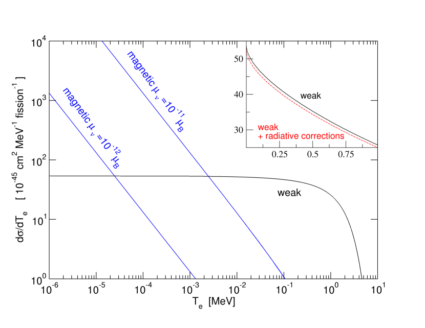
Figure 7: Standard Model weak and magnetic moment electromagnetic contributions to the differential cross section of neutrino-electron scattering averaged over the antineutrino spectrum of fissioning ²³⁵U. The inset plot is the weak correction on the linear scale both with (dashed line) and without (solid line) radiative corrections [454]. Figure from Balantekin and Vassh [60].

The two terms $(d\sigma_{\nu_{\ell}e^{-}}/dT_{e})_{\text{SM}}$ and $(d\sigma_{\nu_{\ell}e^{-}}/dT_{e})_{\text{mag}}$ exhibit quite different dependencies on the experimentally observable electron kinetic energy $T_{e}$, as illustrated in Fig. 7 taken from Balantekin and Vassh [60] (see also Vogel and Engel [511], Beda et al. [84]). One can see that small values of the neutrino magnetic moment can be probed by lowering the electron recoil energy threshold. In fact, considering $T_{e}\ll E_{\nu}$ in Eq. (209) and neglecting the coefficients due to $g_{V}^{\nu_{\ell}}$ and $g_{A}^{\nu_{\ell}}$ in Eq. (206), one can find that $(d\sigma/dT_{e})_{\text{mag}}$ exceeds $(d\sigma/dT_{e})_{\text{SM}}$ for

$$T_{e}\lesssim\frac{\pi^{2}\alpha^{2}}{G_{\text{F}}^{2}m_{e}^{3}}\left(\frac{\bbmu_{\nu}}{\mu_{\text{B}}}\right)^{2}.$$ (210)

IV.4 Effective magnetic moment

In scattering experiments the neutrino is created at some distance from the detector as a flavor neutrino, which is a superposition of massive neutrinos. Therefore, the magnetic moment that is measured in these experiment is not that of a massive neutrino, but it is an effective magnetic moment which takes into account neutrino mixing and the oscillations during the propagation between source and detector [274, 80].

Let us consider an initial neutrino with flavor $\ell=e,\,\mu,\,\tau$, which is described by the flavor state in Eq. (30). The state of the neutrino which is detected through a scattering process at a space-time distance $(\vv{L},T)$ from the source is given by the superposition of massive neutrinos in the first line of Eq. (34). Considering an incoming left-handed neutrino, the amplitude of $\nu_{j}$ production in low-$q^{2}$ electromagnetic scattering of a neutrino which has traveled a space-time distance $(\vv{L},T)$ from a source of $\nu_{\ell}$ is

$$A_{\ell j}(\vv{L},T)\hbox{} \hbox{}\propto\sum_{k}U_{\ell k}^{*}e^{-iE_{k}T+i\vv{p}_{k}\cdot\vv{L}}$$

$$\hbox{}\times\sum_{h_{j}}\overline{u_{j}^{(h_{j})}}\sigma_{\mu\nu}q^{\nu}\left(\bbmu_{jk}+i\bbespilon_{jk}\gamma_{5}\right)u_{k}^{(-)}.$$ (211)

Since for an incoming ultrarelativistic left-handed neutrino the additional $\gamma^{5}$ in the electric dipole term has only the effect of changing a sign (see Eq. (603)), the amplitude of $\nu_{k}\to\nu_{j}$ transitions is proportional to $\bbmu_{jk}-i\bbespilon_{jk}$, leading to

$$A_{\ell j}(\vv{L},T)\propto\sum_{k}U_{\ell k}^{*}e^{-iE_{k}T+i\vv{p}_{k}\cdot\vv{L}}\left(\bbmu_{jk}-i\bbespilon_{jk}\right).$$ (212)

The total cross section of electromagnetic scattering with an electron or a nucleon is given by

$$\sigma_{\nu_{\ell}e^{-}}(\vv{L},T)\propto\sum_{j}|A_{\ell j}(\vv{L},T)|^{2}.$$ (213)

Taking into account that for ultrarelativistic neutrinos $T=L$, from the approximation in Eq. (36) we obtain that the cross section is proportional to the squared effective magnetic moment

$$\bbmu_{\nu_{\ell}}^{2}(L,E_{\nu})=\sum_{j}\left|\sum_{k}U_{\ell k}^{*}e^{-i\Delta{m}^{2}_{kj}L/2E_{\nu}}\left(\bbmu_{jk}-i\bbespilon_{jk}\right)\right|^{2}.$$ (214)

In this expression of the effective $\bbmu_{\nu_{\ell}}$ one can see that in general both the magnetic and electric dipole moments contribute to the elastic scattering. Note also that, as neutrino oscillations discussed in Section II, the effective magnetic moment $\bbmu_{\nu_{\ell}}(L,E_{\nu})$ depends on the neutrino squared-mass differences, not on the absolute values of neutrino masses.

Considering antineutrinos, the mixing of antineutrinos is obtained from that of neutrinos in Eq. (30) with the substitution $U\to U^{*}$. From Eq. (129) it follows that the electric and magnetic moments of antineutrinos are obtained with the substitutions $\bbmu_{jk}\to-\bbmu_{jk}^{*}$ and $\bbespilon_{jk}\to-\bbespilon_{jk}^{*}$. Moreover, we must take into account that incoming antineutrinos are right-handed. Hence, for antineutrinos we have

$$\overline{A}_{\ell j}(\vv{L},T)\hbox{} \hbox{}\propto\sum_{k}U_{\ell k}e^{-iE_{k}T+i\vv{p}_{k}\cdot\vv{L}}$$

$$\hbox{}\times\sum_{h_{j}}\overline{u_{j}^{(h_{j})}}\sigma_{\mu\nu}q^{\nu}\left(\bbmu_{jk}^{*}+i\bbespilon_{jk}^{*}\gamma_{5}\right)u_{k}^{(+)}.$$ (215)

For an incoming ultrarelativistic right-handed neutrino the additional $\gamma^{5}$ in the electric dipole term has no effect (see Eq. (603)) and we obtain

$$\bbmu_{\bar{\nu}_{\ell}}^{2}(L,E_{\nu})=\hbox{} \hbox{}\sum_{j}\left|\sum_{k}U_{\ell k}e^{-i\Delta{m}^{2}_{kj}L/2E_{\nu}}\left(\bbmu_{jk}^{*}+i\bbespilon_{jk}^{*}\right)\right|^{2}$$

$$=\hbox{} \hbox{}\sum_{j}\left|\sum_{k}U_{\ell k}^{*}e^{i\Delta{m}^{2}_{kj}L/2E_{\nu}}\left(\bbmu_{jk}-i\bbespilon_{jk}\right)\right|^{2}.$$ (216)

Therefore, there can be only a phase difference between the terms contributing to $\bbmu_{\nu_{\ell}}^{2}(L,E_{\nu})$ and $\bbmu_{\bar{\nu}_{\ell}}^{2}(L,E_{\nu})$, which is induced by neutrino oscillations.

As discussed in the following Subsection IV.5, the laboratory experiments which are most sensitive to small values of the effective magnetic moment are reactor and accelerator experiments which detect the elastic scattering of flavor neutrinos on electrons at a short distance from the neutrino source. In this case, the value in Eq. (64) of the largest squared-mass difference $\Delta{m}^{2}_{\text{A}}$ in the standard case of three-neutrino mixing is such that $\Delta{m}^{2}_{\text{A}}L/2E_{\nu}\ll 1$. Therefore, it is possible to approximate all the exponentials in Eqs. (214) and (216) with unity and obtain the effective short-baseline magnetic moment of flavor neutrinos and antineutrinos

$$\bbmu_{\nu_{\ell}}^{2}\simeq\hbox{} \hbox{}\bbmu_{\bar{\nu}_{\ell}}^{2}\simeq\sum_{j}\left|\sum_{k}U_{\ell k}^{*}\left(\bbmu_{jk}-i\bbespilon_{jk}\right)\right|^{2}$$

$$=\hbox{} \hbox{}\left[U\left(\bbmu^{2}+\bbespilon^{2}\right)U^{\dagger}+2\operatorname{Im}\!\left(U\,\bbmu\,\bbespilon\,U^{\dagger}\right)\right]_{\ell\ell},$$ (217)

where we took into account that $\bbmu=\bbmu^{\dagger}$ and $\bbespilon=\bbespilon^{\dagger}$. In this approximation the effective magnetic moment is independent of the neutrino energy and from the source-detector distance.

In the following, when we refer to an effective magnetic moment of a flavor neutrino without indication of a source-detector distance $L$ it is implicitly understood that $L$ is small and the effective magnetic moment is given by Eq. (217).

It is interesting to note that flavor neutrinos can have effective magnetic moments even if massive neutrinos are Majorana particles. In this case, since massive Majorana neutrinos do not have diagonal magnetic and electric dipole moments, the effective magnetic moments of flavor neutrinos receive contributions only from the transition dipole moments. For example, in the three-generation case, following Eq. (152), we can write $\bbmu_{jk}$ and $\bbespilon_{jk}$ as

$$\bbmu_{jk}=i\sum_{m=1}^{3}\epsilon_{jkm}\tilde{\bbmu}_{m},\quad\bbespilon_{jk}=i\sum_{m=1}^{3}\epsilon_{jkm}\tilde{\bbespilon}_{m},$$ (218)

with real $\tilde{\bbmu}_{m}$ and $\tilde{\bbespilon}_{m}$. Thus, we obtain

$$\bbmu_{\nu_{\ell}}^{2}\simeq\sum_{k=1}^{3}\left(\tilde{\bbmu}_{k}^{2}+\tilde{\bbespilon}_{k}^{2}\right)-\left|\sum_{k=1}^{3}U_{\ell k}\left(\tilde{\bbmu}_{k}-i\tilde{\bbespilon}_{k}\right)\right|^{2}.$$ (219)

Another case in which the effective magnetic moment does not depend on the neutrino energy and on the source-detector distance is when the source-detector distance is much larger than all the oscillation lengths $L_{kj}=4\pi E_{\nu}/|\Delta{m}^{2}_{kj}|$. In this case the interference terms in Eqs. (214) and (216) are washed out by the finite energy resolution of the detector, leading to

$$\bbmu_{\nu_{\ell}}^{2}\hbox{} \hbox{}(\infty)\simeq\bbmu_{\bar{\nu}_{\ell}}^{2}(\infty)\simeq\sum_{k}|U_{\ell k}|^{2}\sum_{j}\left|\bbmu_{jk}-i\bbespilon_{jk}\right|^{2}$$

$$\hbox{}=\sum_{k}|U_{\ell k}|^{2}\left[(\bbmu^{2})_{kk}+(\bbespilon^{2})_{kk}+2\operatorname{Im}(\bbmu\bbespilon)_{kk}\right].$$ (220)

For three-generations of Majorana neutrinos, from Eq. (218) we obtain

$$\bbmu_{\nu_{\ell}}^{2}(\infty)\simeq\bbmu_{\bar{\nu}_{\ell}}^{2}(\infty)\simeq\sum_{k=1}^{3}\left(1-|U_{\ell k}|^{2}\right)\left(\tilde{\bbmu}_{k}^{2}+\tilde{\bbespilon}_{k}^{2}\right).$$ (221)

Method	Experiment	Limit	CL	Reference
Reactor $\bar{\nu}_{e}$-$e^{-}$	Krasnoyarsk	$\bbmu_{\nu_{e}}<2.4\times 10^{-10}\,\mu_{\text{B}}$	90%	Vidyakin et al. [508]
	Rovno	$\bbmu_{\nu_{e}}<1.9\times 10^{-10}\,\mu_{\text{B}}$	95%	Derbin et al. [166]
	MUNU	$\bbmu_{\nu_{e}}<9\times 10^{-11}\,\mu_{\text{B}}$	90%	Daraktchieva et al. [157]
	TEXONO	$\bbmu_{\nu_{e}}<7.4\times 10^{-11}\,\mu_{\text{B}}$	90%	Wong et al. [522]
	GEMMA	$\bbmu_{\nu_{e}}<2.9\times 10^{-11}\,\mu_{\text{B}}$	90%	Beda et al. [82]
Accelerator $\nu_{e}$-$e^{-}$	LAMPF	$\bbmu_{\nu_{e}}<1.1\times 10^{-9}\,\mu_{\text{B}}$	90%	Allen et al. [32]
Accelerator ($\nu_{\mu},\bar{\nu}_{\mu}$)-$e^{-}$	BNL-E734	$\bbmu_{\nu_{\mu}}<8.5\times 10^{-10}\,\mu_{\text{B}}$	90%	Ahrens et al. [14]
	LAMPF	$\bbmu_{\nu_{\mu}}<7.4\times 10^{-10}\,\mu_{\text{B}}$	90%	Allen et al. [32]
	LSND	$\bbmu_{\nu_{\mu}}<6.8\times 10^{-10}\,\mu_{\text{B}}$	90%	Auerbach et al. [47]
Accelerator ($\nu_{\tau},\bar{\nu}_{\tau}$)-$e^{-}$	DONUT	$\bbmu_{\nu_{\tau}}<3.9\times 10^{-7}\,\mu_{\text{B}}$	90%	Schwienhorst et al. [460]
Solar $\nu_{e}$-$e^{-}$	Super-Kamiokande	$\bbmu_{\text{S}}(E_{\nu}\gtrsim 5\,\text{MeV})<1.1\times 10^{-10}\,\mu_{\text{B}}$	90%	Liu et al. [348]
	Borexino	$\bbmu_{\text{S}}(E_{\nu}\lesssim 1\,\text{MeV})<5.4\times 10^{-11}\,\mu_{\text{B}}$	90%	Arpesella et al. [38]

Table 3: Experimental limits for different neutrino effective magnetic moments.

So far, in this Subsection we have considered the effects of neutrino mixing and oscillations on the effective magnetic moment for neutrinos propagating in vacuum. In the case of solar neutrinos, which have been used by the Super-Kamiokande [348] and Borexino [38] experiments to search for neutrino magnetic moment effects, one must take into account the matter effects discussed in Subsection II.4. The state which describes the neutrinos emerging from the Sun is the following generalization of the state in Eq. (61) which takes into account three-neutrino mixing and the squared-mass hierarchy in Eq. (65):

$$|\nu_{\text{S}}\rangle=\sum_{k=1}^{3}(U_{ek}^{\text{M}})^{*}|\nu_{k}\rangle,$$ (222)

with

$$\hbox{}U_{e1}^{\text{M}}=\cos\vartheta_{13}\cos\vartheta_{\text{M}}^{0},$$ (223)

$$\hbox{}U_{e2}^{\text{M}}=\cos\vartheta_{13}\sin\vartheta_{\text{M}}^{0},$$ (224)

$$\hbox{}U_{e3}^{\text{M}}=U_{e3}=\sin\vartheta_{13}e^{-i\delta_{13}},$$ (225)

where $\vartheta_{\text{M}}^{0}$ is the effective mixing angle at the point of neutrino production inside the Sun. Following the same reasoning that led to Eq. (214), we obtain that the effective magnetic moment measured by an experiment on Earth is

$$\bbmu_{\text{S}}^{2}(L,E_{\nu})=\sum_{j}\left|\sum_{k}(U_{ek}^{\text{M}})^{*}e^{-i\Delta{m}^{2}_{kj}L/2E_{\nu}}\left(\bbmu_{jk}-i\bbespilon_{jk}\right)\right|^{2},$$ (226)

where $L$ is the Sun-Earth distance. Since the Sun-Earth distance is much larger than the oscillation lengths, the interference terms in Eqs. (226) are washed out by the finite energy resolution of the detector and we obtain the effective magnetic moment

$$\bbmu_{\text{S}}^{2}(E_{\nu})=\sum_{k}|U_{ek}^{\text{M}}|^{2}\sum_{j}\left|\bbmu_{jk}-i\bbespilon_{jk}\right|^{2}.$$ (227)

This expression is similar to that in Eq. (220), but takes into account the effective mixing at the point of neutrino production inside the Sun. Note that $\bbmu_{\text{S}}$ depends on the neutrino energy through the dependence of $\vartheta_{\text{M}}^{0}$ on $E_{\nu}$ (see Eq. (54)). As remarked before Eq. (63), in practice we have $\vartheta_{\text{M}}^{0}\simeq\vartheta_{12}$ for $E_{\nu}\lesssim 1\,\text{MeV}$ and $\vartheta_{\text{M}}^{0}\simeq\pi/2$ for $E_{\nu}\gtrsim 5\,\text{MeV}$. Therefore,

$$\bbmu_{\text{S}}(E_{\nu}\lesssim 1\,\text{MeV})\simeq\bbmu_{\nu_{e}}(\infty),$$ (228)

and

$$\bbmu_{\text{S}}^{2}(E_{\nu}\gtrsim\hbox{} \hbox{}5\,\text{MeV})\simeq\cos^{2}\vartheta_{13}\sum_{j}\left|\bbmu_{j2}-i\bbespilon_{j2}\right|^{2}$$

$$\hbox{}+\sin^{2}\vartheta_{13}\sum_{j}\left|\bbmu_{j3}-i\bbespilon_{j3}\right|^{2}.$$ (229)

IV.5 Experimental limits

The constraints on the neutrino magnetic moment in direct laboratory experiments have been obtained so far from the lack of any observable distortion of the recoil electron energy spectrum. Experiments of this type have started in the 50’s at the Savannah River Laboratory where the ${\bar{\nu}_{e}}$-$e^{-}$ elastic scattering process was studied [151, 150, 441] with somewhat controversial results, as discussed by Vogel and Engel [511]. The most significant experimental limits on the effective magnetic moment $\bbmu_{\nu_{e}}$ which have been obtained in reactor ${\bar{\nu}_{e}}$-$e^{-}$ after about 1990 are listed in Tab. 3 (some details of the different experimental setups are reviewed in Broggini et al. [123]).

The current best limit on $\bbmu_{\nu_{e}}$ has been obtained in 2012 in the GEMMA experiment at the Kalinin Nuclear Power Plant (Russia) with a 1.5 kg highly pure germanium detector exposed at a $\bar{\nu}_{e}$ flux of $2.7\times 10^{13}\,\text{cm}^{-2}\,\text{s}^{-1}$ at a distance of 13.9 m from the core of a $3\,\text{GW}_{\text{th}}$ commercial water-moderated reactor [82]. The competitive TEXONO experiment is based at the Kuo-Sheng Reactor Neutrino Laboratory (Taiwan), where a 1.06 kg highly pure germanium detector was exposed to the flux of $\bar{\nu}_{e}$ at a distance of 28 m from the core of a $2.9\,\text{GW}_{\text{th}}$ commercial reactor [522].

Searches for effects of neutrino magnetic moments have been performed also in accelerator experiments. The LAMPF bounds on $\bbmu_{\nu_{e}}$ in Tab. 3 has been obtained with $\nu_{e}$ from $\mu^{+}$ decay [32]. The LAMPF and LSND bounds on $\bbmu_{\nu_{\mu}}$ in Tab. 3 has been obtained with $\nu_{\mu}$ and $\bar{\nu}_{\mu}$ from $\pi^{+}$ and $\mu^{+}$ decay [32, 47]. The DONUT collaboration [460] investigated $\nu_{\tau}$-$e^{-}$ and $\bar{\nu}_{\tau}$-$e^{-}$ elastic scattering, finding the limit on $\bbmu_{\nu_{\tau}}$ in Tab. 3.

Solar neutrino experiments can also search for a neutrino magnetic moment signal by studying the shape of the electron spectrum [80]. The effective magnetic moment $\bbmu_{\text{S}}$ in solar $\nu_{e}$-$e^{-}$ scattering experiments is given in Eq. (227). Table 3 gives the limits on obtained in the Super-Kamiokande experiment [348] for $\bbmu_{\text{S}}(E_{\nu}\gtrsim 5\,\text{MeV})$ and that obtained in the Borexino experiment [38] for $\bbmu_{\text{S}}(E_{\nu}\lesssim 1\,\text{MeV})$ (see Eqs. (229) and (228)).

Information on neutrino magnetic moments has been obtained also with global fits of solar neutrino data [293, 271, 503]. Considering Majorana three-neutrino mixing, Tortola [503] obtained, at 90% CL,

$$\sqrt{|\bbmu_{12}|^{2}+|\bbmu_{23}|^{2}+|\bbmu_{31}|^{2}}<4.0\times 10^{-10}\,\mu_{\text{B}},$$ (230)

from the analysis of solar and KamLAND, and

$$\sqrt{|\bbmu_{12}|^{2}+|\bbmu_{23}|^{2}+|\bbmu_{31}|^{2}}<1.8\times 10^{-10}\,\mu_{\text{B}},$$ (231)

adding the Rovno [166], TEXONO [344] and MUNU [156] constraints.

As we have seen in Subsection IV.3 the neutrino magnetic moment contribution to the $\hbox to0.0pt{\kern-2.5pt$\overset{\scriptscriptstyle(-)}{\phantom{\nu}}$\hss}{{\nu}_{\ell}}$–$e^{-}$ elastic scattering process flips the neutrino helicity. If neutrinos are Dirac particles, this process transforms active left-handed neutrinos into sterile right-handed neutrinos, leading to dramatic effects on the explosion of a core-collapse supernova [155, 399, 243, 331, 71, 395, 513, 49, 50, 61], where there are also contributions from $\hbox to0.0pt{\kern-2.5pt$\overset{\scriptscriptstyle(-)}{\phantom{\nu}}$\hss}{{\nu}_{\ell}}$–$p$ and $\hbox to0.0pt{\kern-2.5pt$\overset{\scriptscriptstyle(-)}{\phantom{\nu}}$\hss}{{\nu}_{\ell}}$–$n$ elastic scattering. Requiring that the entire energy in a supernova collapse is not carried away by the escaping sterile right-handed neutrinos created in the supernova core, Ayala et al. [49, 50] obtained the following upper limit on a generic neutrino magnetic moment:

$$\bbmu_{\nu}\lesssim\left(0.1-0.4\right)\times 10^{-11}\,\mu_{\text{B}},$$ (232)

which is slightly more stringent than the bound $\bbmu_{\nu}\lesssim\left(0.2-0.8\right)\times 10^{-11}\,\mu_{\text{B}}$ obtained by Barbieri and Mohapatra [71].

IV.6 Theoretical considerations

There is a gap of many orders of magnitude between the present experimental limits on neutrino magnetic moments of the order of $10^{-11}\,\mu_{\text{B}}$ (discussed in Subsection IV.5) and the prediction smaller than about $10^{-19}\,\mu_{\text{B}}$ in Eq. (179) of the minimal extension of the Standard Model with right-handed neutrinos. The hope to reach in the near future an experimental sensitivity of this order of magnitude is very weak, taking into account that the experimental sensitivity of reactor ${\bar{\nu}_{e}}$-$e$ elastic scattering experiments have improved by only one order of magnitude during a period of about twenty years (see Vogel and Engel [511], where a sensitivity of the order of $10^{-10}\mu_{\text{B}}$ is discussed). However, the experimental studies of neutrino magnetic moments are stimulated by the hope that new physics beyond the minimally extended Standard Model with right-handed neutrinos might give much stronger contributions.

One of the examples in which it is possible to avoid the neutrino magnetic moment being proportional to a (small) neutrino mass, that would in principle make a neutrino magnetic moment accessible for experimental observations, is realized in the left-right symmetric model with direct right-handed neutrino interactions [467, 300, 362, 85, 469, 189, 349, 437, 154, 388, 116]. In this model there is a new charged boson $W_{R}$ which mediates right-handed charged-current weak interactions and mixes with the Standard Model $W_{L}$ boson which mediates left-handed charged-current weak interactions. The massive gauge bosons states $W_{1}$ and $W_{2}$ are given by

$$\hbox{}W_{1}=W_{L}\cos\xi-W_{R}e^{i\varphi}\sin\xi,$$ (233)

$$\hbox{}W_{2}=W_{L}e^{-i\varphi}\sin\xi+W_{R}\cos\xi,$$ (234)

where $\xi$ is a small mixing angle and $\varphi$ is a possible CP-violating phase. Neglecting the contributions of neutrino masses and the terms suppressed by the small ratio $m_{W_{1}}/m_{W_{2}}$, the magnetic moments of Dirac neutrinos are given by [469, 221]

$$\bbmu_{kj}=\hbox{} \hbox{}\frac{eG_{\text{F}}}{4\sqrt{2}\pi^{2}}\sin 2\xi$$

$$\hbox{}\times\sum_{\ell=e,\mu,\tau}m_{\ell}\left[e^{i\varphi}U^{*}_{\ell k}V_{\ell j}+e^{-i\varphi}V^{*}_{\ell k}U_{\ell j}\right],$$ (235)

where $U$ is the standard mixing matrix of left-handed neutrinos and $V$ is the mixing matrix of right-handed neutrinos. Hence, in this case the neutrino magnetic moments depend on the values of the charged lepton masses. However, one must take into account the coefficient $\sin 2\xi$, which must be very small in order to have small Dirac neutrino masses [154]. For example, in the model of Chang and Mohapatra [135] $\sin\xi\lesssim 10^{-7}$ for $m_{W_{2}}\gtrsim 2.5\,\text{TeV}$ [81, 195, 359], which implies that $\bbmu_{kj}\lesssim 10^{-16}\mu_{\text{B}}$. However, larger values of the magnetic moments have been obtained by Rajpoot [437] by adding to the left-right symmetric model a charged scalar singlet, following the idea of Fukugita and Yanagida [220].

Other interesting possibilities of obtaining neutrino magnetic moments larger than the prediction in Eq. (179) of the minimal extension the Standard Model with right-handed neutrinos have been considered in the literature. For example, the analysis performed by Aboubrahim et al. [9] of the Dirac neutrino magnetic moment in the framework of a Minimal Supersymmetric Standard Model extension with a vectorlike lepton generation showed that a neutrino magnetic moment as large as $\left(10^{-12}-10^{-14}\right)\mu_{\text{B}}$ can be obtained. These values lie within reach of improved laboratory experiments in the future.

Gozdz et al. [252] obtained Majorana transition magnetic moments as large as about $10^{-17}\,\mu_{\text{B}}$, significantly larger than those in Eq. (185), in the framework of the Minimal Supersymmetric Standard Model with $R$-parity violating interactions, constrained by grand unification.

It is possible to estimate a generic relation between the size of a neutrino magnetic moment $\bbmu_{\nu}$ and the corresponding neutrino mass $m_{\nu}$ [512, 75, 407, 160, 87, 86]. Suppose that a large neutrino magnetic moment is generated by physics beyond a minimal extension of the Standard Model at an energy scale characterized by $\Lambda$. This contribution to $\bbmu_{\nu}$ is described by the Feynman diagram in Fig. 4, with the blob representing the effects of new physics beyond the Standard Model. The contribution of this diagram to the magnetic moment is

$$\bbmu_{\nu}\sim\frac{eG}{\Lambda},$$ (236)

where $e$ is the electric charge and $G$ is a combination of coupling constants and loop factors [87, 86]. The diagram of Fig. 4 without the photon line gives a new physics contribution to the neutrino mass of the order

$$\delta{m}_{\nu}\sim G\Lambda.$$ (237)

Combining the estimates (236) and (237), one can get the relation

$$\delta{m}_{\nu}\sim\frac{\Lambda^{2}}{2m_{e}}\frac{\bbmu_{\nu}}{\mu_{\text{B}}}=\frac{\bbmu_{\nu}}{10^{-18}\mu_{\text{B}}}\left(\frac{\Lambda}{\text{TeV}}\right)^{2}\,\text{eV}$$ (238)

between the new physics contribution to the neutrino mass and the neutrino magnetic moment.

It follows that, generally, in theoretical models that predict large values for the neutrino magnetic moment, simultaneously large contributions to the neutrino mass arise. Therefore, a particular fine tuning is needed to get a large value for the neutrino magnetic moment while keeping the neutrino mass within experimental bounds, unless the ratio $m_{\nu}/\bbmu_{\nu}$ is suppressed by a symmetry. Voloshin [512] proposed a $\text{SU}(2)_{\nu}$ under which the neutrino and antineutrino fields, $\nu$ and $\nu^{c}$, transform as a doublet. Taking into account that fermion fields anticommute, a Dirac mass term can be written as

$$\overline{\nu}\nu=-\nu^{T}\overline{\nu}^{T}=-\nu^{T}\mathcal{C}^{\dagger}\mathcal{C}\overline{\nu}^{T}=-\nu^{T}\mathcal{C}^{\dagger}\nu^{c},$$ (239)

and a magnetic moment term can be written as

$$\overline{\nu}\sigma_{\alpha\beta}\nu=-\nu^{T}\sigma_{\alpha\beta}^{T}\overline{\nu}^{T}=\nu^{T}\mathcal{C}^{\dagger}\sigma_{\alpha\beta}\nu^{c}.$$ (240)

One can see that the mass term is invariant under the change $\nu\leftrightarrows\nu^{c}$, whereas the magnetic moment term changes sign. Therefore, the magnetic moment term is a singlet under the $\text{SU}(2)_{\nu}$ symmetry, whereas the mass term transforms as a triplet and is forbidden. If, as it happens in a realistic model, the $\text{SU}(2)_{\nu}$ symmetry is broken and if this breaking is small, the ratio $m_{\nu}/\bbmu_{\nu}$ is also small, giving a natural way to obtain a magnetic moment of the order of $\sim 10^{-11}\mu_{\text{B}}$ without contradictions with the neutrino mass experimental constraints. Several possibilities based on the general idea of Voloshin [512] were considered by Leurer and Marcus [343], Babu and Mohapatra [52], Georgi and Randall [232], Ecker et al. [196], Chang et al. [134], Barbieri and Mohapatra [72].

Another idea of neutrino mass suppression without suppression of the neutrino magnetic moment was discussed by Barr et al. [75] within the Zee model [531], which is based on the Standard Model gauge group $\text{SU}(2)_{L}\times\text{U}(1)_{Y}$ and contains at least three Higgs doublets and a charged field which is a singlet of $\text{SU}(2)_{L}$. For this kind of models there is a suppression of the neutrino mass diagram, while the magnetic moment diagram is not suppressed.

Bell et al. [88], Davidson et al. [160], Bell et al. [87], Bell [86] derived “natural” upper bounds for the magnetic moments of Dirac and Majorana neutrinos generated by new physics above the electroweak scale. They considered an effective low-energy theory in which the effects of the new physics above the electroweak scale are described by high-dimension nonrenormalizable operators whose coefficients are not fine-tuned. The low-energy effective Lagrangian must respect the Standard Model $\text{SU}(2)_{L}\times\text{U}(1)_{Y}$ symmetry and is constructed with Standard Model fields plus right-handed neutrino fields $\nu_{R}$ (with implicit flavor indices), in order to have Dirac neutrino masses. This low-energy effective Lagrangian can be written as

$$\mathcal{L}_{\text{eff}}=\sum_{n,j}\frac{\mathcal{C}^{n}_{j}(\mu)}{\Lambda^{n-4}}\mathcal{O}_{j}^{(n)}(\mu)+\text{H.c.},$$ (241)

where $\mu$ is the renormalization scale, $n\geq 4$ denotes the operator dimension and $j$ runs over independent operators of a given dimension. For $n=4$, a Dirac neutrino mass arises from the operator $\mathcal{O}^{(4)}_{1}=\overline{L}\tilde{\Phi}\nu_{R}$, where ${\tilde{\Phi}}=i\sigma_{2}\Phi^{*}$. For $n=6$ there are two operators which generate, after electroweak symmetry breaking, the magnetic moment operator $\overline{\nu}\sigma_{\alpha\beta}\nu F^{\alpha\beta}$. These operators can generate a contribution to the neutrino mass operator $\mathcal{O}^{(4)}_{1}$ through loop diagrams. Using dimensional analysis, Bell et al. [88] estimated that the corresponding contribution $\delta{m}_{\nu}^{(4)}$ to the Dirac neutrino mass is given by

$$\delta{m}_{\nu}^{(4)}\sim\frac{\alpha}{16\pi}\frac{\Lambda^{2}}{m_{e}}\frac{\bbmu_{\nu}^{\text{D}}}{\mu_{\text{B}}}.$$ (242)

Apart from the different coefficient, the dependence on $\Lambda$ and $\mu_{\text{B}}$ is the same as in Eq. (238). The ${\Lambda}^{2}$ dependence is due to the quadratic divergence in the renormalization of the dimension-four neutrino mass operator. Imposing that $\delta{m}_{\nu}$ is smaller than the neutrino mass $m_{\nu}$, we obtain

$$\bbmu_{\nu}^{\text{D}}\lesssim 3\times 10^{-15}\,\mu_{\text{B}}\left(\frac{m_{\nu}}{\text{eV}}\right)\left(\frac{\text{TeV}}{\Lambda}\right)^{2}.$$ (243)

For $\Lambda\sim 1\,\text{TeV}$ and $m_{\nu}\lesssim 1\,\text{eV}$, one obtains $\bbmu_{\nu}^{\text{D}}\lesssim 3\times 10^{-15}\,\mu_{\text{B}}$, which is some orders of magnitude stronger than the experimental constraints in Tab. 3.

Bell et al. [88] noted that if the scale $\Lambda$ is close to the electroweak scale, an important contribution to the neutrino mass can arise also from an $n=6$ operator. In order to obtain a natural upper bound on $\bbmu_{\nu}^{\text{D}}$ they assumed that at the scale $\Lambda$ the coefficient of the $n=6$ mass operator is zero, so that the contribution to the neutrino mass is generated entirely by radiative corrections involving insertions of the $n=6$ magnetic moment operators. Solving the renormalization group equations from the scale $\Lambda$ to the electroweak scale, they found the following relation between the contribution $\delta{m}_{\nu}^{(6)}$ neutrino mass and the neutrino magnetic moment:

$$\frac{\bbmu_{\nu}^{\text{D}}}{\mu_{\text{B}}}=\frac{16\sqrt{2}G_{\text{F}}m_{e}\sin^{4}\theta_{W}}{9\alpha^{2}|f|\ln\left(\Lambda/v\right)}\,\delta{m}_{\nu}^{(6)},$$ (244)

where $\alpha$ is the fine structure constant, $v$ is the vacuum expectation value of the Higgs doublet,

$$f=1-r-\frac{2}{3}\tan^{2}\theta_{W}-\frac{1}{3}(1+r)\tan^{4}\theta_{W},$$ (245)

and $r$ is a ratio of effective operator coefficients defined at the scale $\Lambda$ which is of order unity without fine-tuning. If the neutrino magnetic moment is generated by new physics at a scale $\Lambda\sim 1\,\text{TeV}$ and the corresponding contribution to the neutrino mass is $\delta{m}_{\nu}^{(6)}\lesssim 1\,\text{eV}$, then $\bbmu_{\nu}\lesssim 8\times 10^{-15}\mu_{\text{B}}$. Also this bound is some orders of magnitude stronger than the experimental constraints in Tab. 3.

Following a similar method, Bell et al. [87] calculated natural upper bounds for the transition magnetic moments of Majorana neutrinos (see also Davidson et al. [160]). They found that the most general naturalness upper bounds for the Majorana transition magnetic moments in the flavor basis are given by

$$\mu_{\ell\ell^{\prime}}^{\text{M}}\lesssim 4\times 10^{-9}\,\mu_{\text{B}}\left(\frac{M_{\ell\ell^{\prime}}^{\text{M}}}{\text{eV}}\right)\left(\frac{\text{TeV}}{\Lambda}\right)^{2}\left|\frac{m_{\tau}^{2}}{m_{\ell}^{2}-m_{\ell^{\prime}}^{2}}\right|,$$ (246)

where $M_{\ell\ell^{\prime}}^{\text{M}}$ is the Majorana neutrino mass matrix in the flavor basis. For Majorana neutrinos the flavor and mass bases are related by a transformation similar to that in Eq. (21): $(U^{T}M^{\text{M}}U)_{kj}=m_{k}\delta_{kj}$, where $U$ is the neutrino mixing matrix. For the magnetic moments we have

$$\mu_{kj}^{\text{M}}=\sum_{\ell,\ell^{\prime}}U_{\ell k}\mu_{\ell\ell^{\prime}}^{\text{M}}U_{\ell^{\prime}j}.$$ (247)

The limits (246) are much weaker than those in the Dirac case, because for a Majorana neutrino the magnetic moment contribution to the mass is Yukawa suppressed. Hence, if a neutrino transition magnetic moment larger than about $10^{-14}\mu_{\text{B}}$ is observed in an experiment, it would indicate that it is plausible that neutrinos are Majorana rather than Dirac particles.

Let us emphasize that the natural upper bounds on neutrino magnetic moments derived by Bell et al. [88], Davidson et al. [160], Bell et al. [87], Bell [86] apply in models with new physics well above the electroweak scale, for which only the first terms of the effective Lagrangian expansion in Eq. (241) are not negligible. This is not the case, for example, in the model discussed by Aboubrahim et al. [9], in which there is new physics at the electroweak scale.

An unusual case of a large observable effect of the small magnetic moments in Eq. (179) is that of $\bar{\nu}_{e}$–$e^{-}$ elastic scattering in large extra dimension brane-bulk models with three bulk neutrinos discussed by Mohapatra et al. [385]. They showed that the magnetic moment contribution to $\bar{\nu}_{e}$–$e^{-}$ elastic scattering due to the tower of Kaluza-Klein right-handed neutrino states, each contribution with a magnetic moment given by Eq. (179), can be comparable with that of a single neutrino in four-dimensional space-time with magnetic moment of the order of $10^{-10}\,\mu_{\text{B}}$ and the different shapes of the spectra can distinguish the two cases. Hence, $\bar{\nu}_{e}$–$e^{-}$ elastic scattering experiments searching for the effects of neutrino magnetic moments can probe the existence of large extra dimensions.

V Radiative decay and related processes

The magnetic and electric (transition) dipole moments of neutrinos, as well as possible very small electric charges (millicharges), describe direct couplings of neutrinos with photons which induce several observable decay processes. In this Section we discuss the decay processes generated by the diagrams in Fig. 8: the diagram in Fig. 8 generates neutrino radiative decay $\nu_{i}\to\nu_{f}+\gamma$ and the processes of neutrino Cherenkov radiation and spin light ($SL\nu$) of a neutrino propagating in a medium; the diagram in Fig. 8 generates photon (plasmon) decay to an neutrino-antineutrino pair in a plasma ($\gamma^{*}\to\nu\bar{\nu}$).

In Subsections V.1 and V.2 we review neutrino radiative decay in vacuum and in matter, respectively. In Subsection V.3 we discuss neutrino Cherenkov radiation. In Subsection V.4 we consider the process of plasmon decay into a neutrino-antineutrino pair, which can be important in dense astrophysical environments as the interior of stars. In Subsection V.5 we review the spin light process of a neutrino propagating in a medium.

Figure 8: Feynman diagrams for neutrino radiative decay and Cherenkov radiation 8 and plasmon decay 8.

V.1 Radiative decay

If the masses of neutrinos are nondegenerate, the radiative decay of a heavier neutrino $\nu_{i}$ into a lighter neutrino $\nu_{f}$ (with $m_{i}>m_{f}$ ) with emission of a photon,

$$\nu_{i}\to\nu_{f}+\gamma,$$ (248)

may proceed in vacuum [467, 362, 332, 414, 244, 530, 408, 469]. Early discussions of the possible role of neutrino radiative decay in different astrophysical and cosmological settings can be found in Dicus et al. [170], Sato and Kobayashi [455], Stecker [478], Kimble et al. [303], Melott and Sciama [372], De Rujula and Glashow [162].

The neutrino radiative decay process is generated by the interaction in Fig. 5 with a real photon. The decay amplitude is given by

$$\hbox{}\langle\nu_{f}(p_{f},h_{f}),\gamma(q,\varepsilon)|\int d^{4}x\mathcal{H}_{\text{em}}^{(\nu)}(x)|\nu_{i}(p_{i},h_{i})\rangle$$

$$=\hbox{} \hbox{}(2\pi)^{4}\delta^{4}(q-p_{i}+p_{f})\overline{u^{(h_{f})}}(p_{f})\Lambda^{fi}_{\mu}(q)u^{(h_{i})}(p_{i})\varepsilon^{\mu},$$ (249)

where $p_{i}$ ($p_{f}$) and $h_{i}$ ($h_{f}$) are the four-momentum and helicity of the initial (final) neutrino and $q$ and $\varepsilon$ are the four-momentum and polarization four-vectors of the photon. The Dirac $\delta$-function implements energy-momentum conservation.

Taking into account that for a real photon

$$q^{2}=0\quad\text{and}\quad\varepsilon^{\mu}q_{\mu}=0,$$ (250)

from the general expression of $\Lambda_{\mu}(q)$ for Dirac neutrinos in Eq. (116) and from Eq. (120), we obtain

$$\Lambda^{fi}_{\mu}(q)\varepsilon^{\mu}=\mathbbm{q}_{fi}\not{\epsilon}-i\sigma_{\mu\nu}\varepsilon^{\mu}q^{\nu}\left(\bbmu_{fi}+i\bbespilon_{fi}\gamma_{5}\right),$$ (251)

where $\mathbbm{q}_{fi}\neq 0$ only if neutrinos are millicharged particles (see Subsection VII.1). Therefore, the radiative decay of a neutrino $\nu_{i}$ into a lighter neutrino $\nu_{f}$ depends on the corresponding transition charge, magnetic moment and electric moment. Assuming $\mathbbm{q}_{fi}=0$, the decay rate in the rest frame (rf) of the decaying neutrino $\nu_{i}$ is given by (see Raffelt [427, 433, 434])

$$\Gamma_{\nu_{i}\to\nu_{f}+\gamma}^{\text{rf}}=\frac{1}{8\pi}\left(\frac{m_{i}^{2}-m_{f}^{2}}{m_{i}}\right)^{3}\left(|\bbmu_{fi}|^{2}+|\bbespilon_{fi}|^{2}\right).$$ (252)

This expression is valid for both Dirac and Majorana neutrinos, because both can have transition magnetic and electric moments and the corresponding expression (143) for $\Lambda_{\mu}(q)$ in the Majorana case is equivalent to that in Eq. (116) for Dirac neutrinos.

The transition magnetic and electric dipole moments of Dirac neutrinos in the minimal extension of the Standard Model with right-handed neutrinos are given approximately by Eq. (181). In this case, the radiative decay rate is given by [469]

$$\Gamma_{\nu^{\text{D}}_{i}\to\nu^{\text{D}}_{f}+\gamma}^{\text{rf}}\simeq\hbox{} \hbox{}\frac{\alpha}{2}\left(\frac{3G_{\text{F}}}{32\pi^{2}}\right)^{2}\left(\frac{m^{2}_{i}-m^{2}_{f}}{m_{i}}\right)^{3}\left(m^{2}_{i}+m^{2}_{f}\right)$$

$$\hbox{}\times\left|\sum_{\ell=e,\mu,\tau}U^{*}_{\ell i}U_{\ell f}\,\frac{m_{\ell}^{2}}{m_{W}^{2}}\right|^{2}.$$ (253)

The radiative decay rate is suppressed by the small phase space due to the smallness of neutrino masses, by the proportionality of the magnetic (electric) transition moment to the sum (difference) of the masses of the two neutrinos involved in the decay and by a coefficient which is smaller than $(m_{\tau}/m_{W})^{4}\simeq 2\times 10^{-7}$. Note, however, that there are models (see, for instance, Petcov [415], Aboubrahim et al. [10, 9]) in which the neutrino radiative decay rate (as well as the magnetic moment discussed in Section IV) of a Dirac neutrino are much larger than those predicted in the minimally extended Standard Model.

The expression of the decay rate for Majorana neutrinos in the simplest extensions of the Standard Model (without taking into account model-dependent contributions of the scalar sector) can be derived from the expressions in Eqs. (193) and (194) of the Majorana magnetic and electric transition moments [469]:

$$\Gamma_{\nu^{\text{M}}_{i}\to\nu^{\text{M}}_{f}+\gamma}^{\text{rf}}\simeq\hbox{} \hbox{}\alpha\left(\frac{3G_{\text{F}}}{32\pi^{2}}\right)^{2}\left(\frac{m^{2}_{i}-m^{2}_{f}}{m_{i}}\right)^{3}$$

$$\hbox{}\times\left\{\left(m_{i}+m_{f}\right)^{2}\left|\sum_{\ell=e,\mu,\tau}U^{*}_{\ell i}U_{\ell f}\,\frac{m_{\ell}^{2}}{m_{W}^{2}}\right|^{2}\right.$$

$$\hbox{}\left.-4m_{i}m_{f}\left(\operatorname{Re}\left[\sum_{\ell=e,\mu,\tau}U^{*}_{\ell i}U_{\ell f}\,\frac{m_{\ell}^{2}}{m_{W}^{2}}\right]\right)^{2}\right\}.$$ (254)

In the case of CP conservation, from Eqs. (198) and (199) it follows that the decay process is induced purely by the neutrino electric or magnetic transition dipole moment if the CP phases of $\nu_{i}$ and $\nu_{f}$ are, respectively, equal or opposite.

For numerical estimations it is convenient to express the lifetime $\tau_{\nu_{i}\to\nu_{f}+\gamma}=\Gamma_{\nu_{i}\to\nu_{f}+\gamma}^{-1}$ in the following form:

$$\tau_{\nu_{i}\to\nu_{f}+\gamma}^{\text{rf}}\simeq 0.19\left(\frac{m_{i}^{2}}{m^{2}_{i}-m^{2}_{f}}\right)^{3}\left(\frac{\text{eV}}{m_{i}}\right)^{3}\left(\frac{\mu_{\text{B}}}{\bbmu_{fi}^{\text{eff}}}\right)^{2}\text{s},$$ (255)

with the neutrino effective magnetic moment

$$\bbmu_{fi}^{\text{eff}}=\sqrt{|\bbmu_{fi}|^{2}+|\bbespilon_{fi}|^{2}}.$$ (256)

Since $\bbmu_{fi}^{\text{eff}}$ is very small, the lifetime in Eq. 255 is very long. Indeed, in the case of Dirac neutrinos in the minimal extension of the Standard Model with right-handed neutrinos, considering only the dominant $\tau$ contribution in Eq. (253) and neglecting $m_{f}$, we obtain

$$\tau_{\nu^{\text{D}}_{i}\to\nu^{\text{D}}_{f}+\gamma}^{\text{rf}}\simeq\frac{6.2\times 10^{43}\,\text{s}}{|U_{\tau i}|^{2}|U_{\tau f}|^{2}}\left(\frac{\text{eV}}{m_{i}}\right)^{5}.$$ (257)

For $m_{i}\lesssim 1\,\text{eV}$, this lifetime is much larger than the age of the Universe, which is about $4.3\times 10^{17}\,\text{s}$ [93].

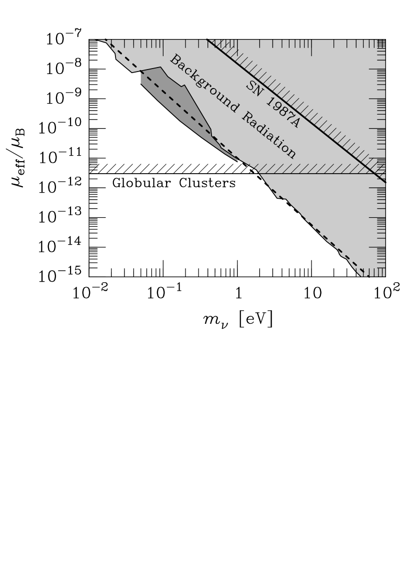
Figure 9: Astrophysical limits on neutrino transition moments. Figure from Raffelt [434].

The neutrino radiative decay can be constrained by the absence of decay photons in reactor $\bar{\nu}_{e}$ and solar $\nu_{e}$ fluxes. The limits on $\bbmu_{fi}^{\text{eff}}$ that are obtained from these considerations are much weaker than those obtained from neutrino scattering terrestrial experiments. Stronger constraints on $\bbmu_{fi}^{\text{eff}}$ (though still weaker than those obtained in terrestrial experiments) are obtained from the neutrino decay limit set by SN 1987A [308, 291] and from the measurements of the diffuse cosmic infrared background and those of the cosmic microwave background [152, 455, 168, 163, 478, 303, 173, 442, 108, 432, 366, 382]. These limits, shown in Fig. 9, can be expressed as (see Raffelt [427, 433, 434])

$$\frac{\bbmu_{fi}^{\text{eff}}}{\mu_{\text{B}}}<\left\{\begin{array}[]{ll}0.9{\times}10^{-1}\left(\text{eV}/m_{\nu}\right)^{2}&\text{Reactor ($\bar{\nu}_{e}$)},\\ 0.5{\times}10^{-5}\left(\text{eV}/m_{\nu}\right)^{2}&\text{Sun ($\nu_{e}$)},\\ 1.5{\times}10^{-8}\left(\text{eV}/m_{\nu}\right)^{2}&\text{SN 1987A (all flavors)},\\ 1.0{\times}10^{-11}\left(\text{eV}/m_{\nu}\right)^{9/4}&\begin{array}[]{l}\text{Cosmic background}\\ \text{(all flavors)}.\end{array}\end{array}\right.$$ (258)

Let us also recall the studies of the effect of neutrino radiative decay on primordial Big-Bang Nucleosynthesis in Sato and Kobayashi [455], Dicus et al. [168], Miyama and Sato [383], Audouze et al. [46], Terasawa et al. [497] (see also the review by Dolgov [172]).

Until now in this Subsection we considered the standard framework of three-neutrino mixing in which there are three massive neutrinos, but it is possible that additional massive neutrinos which are mainly sterile exist, as explained in Subsection II.6. The radiative decay of heavy massive neutrinos is a topic of current interest in view of the recent indication of an astrophysical monochromatic X-ray line at and energy of about 3.5 keV [126, 119], which could be due to the radiative decay of a heavy neutrino with a mass of about 7 keV [7, 510, 282] in agreement with the prediction of the $\nu$MSM (see Boyarsky et al. [120], Kusenko [320], Drewes [182], Boyarsky et al. [118]). In fact, from energy-momentum conservation in the two-body decay (248) the energy of the emitted photon in the rest frame of the decaying neutrino $\nu_{i}$ is given by

$$E_{\gamma}=\frac{m_{i}^{2}-m_{f}^{2}}{2m_{i}}\simeq\frac{m_{i}}{2}\quad\text{for}\quad m_{i}\gg m_{f}.$$ (259)

Let us first consider the radiative decay of Dirac neutrinos. Using Eq. (252), the transition dipole moments in Eq. (192) imply the decay rates

$$\hbox{}\Gamma_{\nu^{\text{D}}_{i}\to\nu^{\text{D}}_{f}+\gamma}^{\text{rf}}\simeq\frac{\alpha}{2}\left(\frac{3G_{\text{F}}}{16\pi^{2}}\right)^{2}\left(\frac{m^{2}_{i}-m^{2}_{f}}{m_{i}}\right)^{3}\left(m^{2}_{i}+m^{2}_{f}\right)$$

$$\hbox{}\hskip 28.45274pt\times\left|\sum_{n=1}^{N_{s}}U^{*}_{s_{n}i}U_{s_{n}f}+\frac{1}{2}\sum_{\ell=e,\mu,\tau}U^{*}_{\ell i}U_{\ell f}\frac{m_{\ell}^{2}}{m_{W}^{2}}\right|^{2}.$$ (260)

The inequality (79) suppresses quadratically the sterile contribution to the decays between two standard massive neutrinos ($k,j\leq 3$) and the decays between two nonstandard massive neutrinos are strongly suppressed by Eqs. (78) and (80). On the other hand, the decay of a nonstandard heavy massive neutrino $\nu_{h}$ with $h\geq 4$ into a lighter standard massive neutrino $\nu_{l}$ with $l\leq 3$ can be significant if $|U_{s_{h-3}l}|$ is not too small. Neglecting the small contributions due to the charged lepton masses and considering $m_{h}\gg m_{l}$, we have

$$\Gamma_{\nu^{\text{D}}_{h}\to\nu^{\text{D}}_{l}+\gamma}^{\text{rf}}\simeq\frac{\alpha}{2}\left(\frac{3G_{\text{F}}}{16\pi^{2}}\right)^{2}m_{h}^{5}\,|U_{s_{h-3}h}|^{2}|U_{s_{h-3}l}|^{2}.$$ (261)

If the mixing of $\nu_{s_{h-3}}$ with the three light neutrinos is dominated by $|U_{s_{h-3}l}|^{2}$, we can define an approximate effective mixing angle $\vartheta_{hl}$ such that

$$\cos^{2}\vartheta_{hl}\simeq|U_{s_{h-3}h}|^{2},\quad\sin^{2}\vartheta_{hl}\simeq|U_{s_{h-3}l}|^{2},$$ (262)

and we can write the decay rate as

$$\Gamma_{\nu^{\text{D}}_{h}\to\nu^{\text{D}}_{l}+\gamma}^{\text{rf}}\simeq\frac{\alpha}{2}\left(\frac{3G_{\text{F}}}{32\pi^{2}}\right)^{2}m_{h}^{5}\,\sin^{2}2\vartheta_{hl}.$$ (263)

This approximation is convenient for the analysis of experimental data, because the decay rate depends on only two unknown parameters, the heavy neutrino mass $m_{h}$ and the effective mixing angle $\vartheta_{hl}$.

Let us consider now the decay of heavy nonstandard massive neutrinos in the Majorana framework, which applies to the $\nu$MSM explanation of the astrophysical 3.5 keV X-ray line mentioned above (see Boyarsky et al. [120], Kusenko [320], Drewes [182], Boyarsky et al. [118]). The decay rates are generalizations of those in Eq. (254) taking into account the transition magnetic and electric moments in Eqs. (200) and (201). For simplicity, let us consider only the decay of a heavy neutrino $\nu_{h}$ with $h\geq 4$ into a light neutrino $\nu_{l}$ with $l\leq 3$. Neglecting the small contributions due to the charged lepton masses and considering $m_{h}\gg m_{l}$ we obtain

$$\Gamma_{\nu^{\text{M}}_{h}\to\nu^{\text{M}}_{l}+\gamma}^{\text{rf}}\simeq\alpha\left(\frac{3G_{\text{F}}}{16\pi^{2}}\right)^{2}m_{h}^{5}\,|U_{s_{h-3}h}|^{2}|U_{s_{h-3}l}|^{2}.$$ (264)

This expression is twice of that in Eq. (261) in the Dirac case. Under the approximation (262) we obtain

$$\Gamma_{\nu^{\text{M}}_{h}\to\nu^{\text{M}}_{l}+\gamma}^{\text{rf}}\simeq\alpha\left(\frac{3G_{\text{F}}}{32\pi^{2}}\right)^{2}m_{h}^{5}\,\sin^{2}2\vartheta_{hl}.$$ (265)

This expression is typically used in the phenomenological studies of heavy neutrino radiative decay in the $\nu$MSM model (see Boyarsky et al. [120], Kusenko [320], Drewes [182], Boyarsky et al. [118]).

Let us finally mention that the radiative decay of heavy neutrinos may be observable also in hadron collider experiments [117].

V.2 Radiative decay in matter

As explained in Subsection II.4, the evolution of neutrinos propagating in matter is affected by the potential generated by the coherent forward elastic scattering with the particles in the medium. It turns out that the coherent interaction with an electron background induces the radiative decay in Eq. (248) with a rate that is not suppressed by the GIM mechanism as the decay rate in vacuum in Eq. (253) [176]. Following the approach of Giunti et al. [235], the process of radiative decay in an electron background can be represented by the two Feynman diagrams in Fig. 10 which are obtained from the CC potential diagram in Fig. 1 attaching a final photon line at the initial or final electron line. As in the case of the calculation of the potential (see Giunti and Kim [234]), the coherent contribution of the electron background is obtained by considering equal initial and final four-momenta of the electron. The resulting decay rate in the rest frame of the electron background is

$$\Gamma_{\nu_{i}\to\nu_{f}+\gamma}^{\text{mat}}=\frac{\alpha G_{\text{F}}^{2}N_{e}^{2}}{2m_{e}^{2}}\left(\frac{m_{i}^{2}-m_{f}^{2}}{m_{i}}\right)|U_{ei}|^{2}|U_{ef}|^{2}F(v_{i}),$$ (266)

where $N_{e}$ is the electron number density, $v_{i}=|\vv{p}_{i}|/E_{i}$ is the velocity of the initial neutrino, and

$$F(v_{i})=\sqrt{1-v_{i}^{2}}\left[\frac{2}{v_{i}}\ln\left(\frac{1+v_{i}}{1-v_{i}}\right)-3+\frac{m_{f}^{2}}{m_{i}^{2}}\right].$$ (267)

In the realistic case of ultrarelativistic initial neutrinos, we have

$$F(v_{i})\xrightarrow[v_{i}\to 1]{}4\,m_{i}/E_{i}.$$ (268)

Note that the matter-induced radiative decay is independent of the Dirac or Majorana nature of neutrinos, because it is generated by the coherent weak interactions with matter, which are the same for left-handed neutrinos.

Figure 10: Feynman diagrams of the coherent contribution of background electrons to the radiative decay $\nu_{i}(p_{i})\to\nu_{f}(p_{f})+\gamma(q)$ in matter.

Neglecting the final neutrino mass in Eq. (266), the numerical value of the lifetime $\tau_{\nu_{i}\to\nu_{f}+\gamma}^{\text{mat}}=(\Gamma_{\nu_{i}\to\nu_{f}+\gamma}^{\text{mat}})^{-1}$ for ultrarelativistic initial neutrinos is given by

$$\tau_{\nu_{i}\to\nu_{f}+\gamma}^{\text{mat}}\simeq\frac{4.0\times 10^{30}\,\text{s}}{|U_{ei}|^{2}|U_{ef}|^{2}}\left(\frac{\text{eV}}{m_{i}}\right)^{2}\left(\frac{E_{i}}{\text{MeV}}\right)\left(\frac{N_{\text{A}}\,\text{cm}^{-3}}{N_{e}}\right)^{2}.$$ (269)

In order to compare the radiative lifetime in matter in Eq. (269) with the radiative lifetime in vacuum in Eq. (257), obtained in the minimal extension of the Standard Model with right-handed neutrinos, we must take into account the Lorentz boost factor $\gamma_{i}=E_{i}/m_{i}$ from the rest frame of the decaying neutrino to the rest frame of the electron background:

$$\frac{\tau_{\nu_{i}\to\nu_{f}+\gamma}^{\text{mat}}}{\gamma_{i}\tau_{\nu^{\text{D}}_{i}\to\nu^{\text{D}}_{f}+\gamma}^{\text{rf}}}\simeq\hbox{} \hbox{}1.1\times 10^{-19}\left(\frac{|U_{\tau i}|^{2}|U_{\tau f}|^{2}}{|U_{ei}|^{2}|U_{ef}|^{2}}\right)$$

$$\hbox{}\times\left(\frac{m_{i}}{\text{eV}}\right)^{4}\left(\frac{N_{\text{A}}\,\text{cm}^{-3}}{N_{e}}\right)^{2}.$$ (270)

Therefore, the radiative decay rate in an electron background is many orders of magnitude larger than the radiative decay rate in vacuum in the minimal extension of the Standard Model with right-handed neutrinos. However, the large value of the lifetime in Eq. (269) indicate that it is very difficult, if not impossible, to find a realistic application of this effect.

So far we have considered the radiative decay rate in a background of electrons, assuming that the temperature is not very high. For a temperature $T\gg m_{e}$ both electrons and positrons are present in the background and the radiative decay rate is given by D’Olivo et al. [176]

$$\Gamma_{\nu_{i}\to\nu_{f}+\gamma}^{(T\gg m_{e})}=\frac{\alpha G_{\text{F}}^{2}T^{4}}{72}\left(\frac{m_{i}^{2}-m_{f}^{2}}{m_{i}}\right)|U_{ei}|^{2}|U_{ef}|^{2}F(v_{i}).$$ (271)

Neglecting the final neutrino mass, for ultrarelativistic initial neutrinos we have

$$\tau_{\nu_{i}\to\nu_{f}+\gamma}^{(T\gg m_{e})}\simeq\frac{1.2\times 10^{16}\,\text{s}}{|U_{ei}|^{2}|U_{ef}|^{2}}\left(\frac{\text{eV}}{m_{i}}\right)^{2}\left(\frac{E_{i}}{\text{MeV}}\right)\left(\frac{\text{MeV}}{T}\right)^{4}.$$ (272)

Therefore, in this case the radiative decay in matter is enormously faster than that in vacuum in the minimal extension of the Standard Model with right-handed neutrinos:

$$\frac{\tau_{\nu_{i}\to\nu_{f}+\gamma}^{(T\gg m_{e})}}{\gamma_{i}\tau_{\nu^{\text{D}}_{i}\to\nu^{\text{D}}_{f}+\gamma}^{\text{rf}}}\simeq\hbox{} \hbox{}3.3\times 10^{-34}\left(\frac{|U_{\tau i}|^{2}|U_{\tau f}|^{2}}{|U_{ei}|^{2}|U_{ef}|^{2}}\right)$$

$$\hbox{}\times\left(\frac{m_{i}}{\text{eV}}\right)^{4}\left(\frac{\text{MeV}}{T}\right)^{4}.$$ (273)

Let us finally mention that: Nieves and Pal [394] calculated the radiative decay rate of neutrinos propagating in a thermal background of electrons and photons, taking into account the effect of the stimulated emission of photons in the thermal bath; Grasso and Semikoz [254] calculated the decay rate of a neutrino induced by the emission or absorption of a photon in a plasma taking into account the effective mass of the photons (plasmons); Skobelev [474], Zhukovsky et al. [533], Kachelriess and Wunner [294] calculated the radiative decay rate of neutrinos propagating in magnetic fields; Ternov and Eminov [498, 499] calculated the radiative decay rate of neutrinos propagating in a magnetized plasma.

V.3 Cherenkov radiation

It is well known that a charged particle moving through a medium at a velocity greater than the speed of light in the medium, $v>c/n$ ($n$ is the medium refractive index), can emit Cherenkov radiation. In the same way, neutrinos with a magnetic moment (and/or an electric dipole moment) propagating in a medium with a velocity larger than the velocity of light in the medium can emit Cherenkov radiation. This possibility was first discussed by Radomski [425], who studied a solution of the solar neutrino problem in which the rate of solar neutrino detection is lowered by the loss of energy of the neutrinos due to the emission of Cherenkov radiation in the solar matter. However, the effect was found to be too small to reduce significantly the solar neutrino flux.

The Cerenkov radiation is the helicity flip process

$$\nu_{L}(p)\rightarrow\nu_{R}(p^{\prime})+\gamma(k),$$ (274)

where $\nu_{L}(p)$ and $\nu_{R}(p^{\prime})$ denote the initial and final states of the same neutrino with negative and positive helicities, respectively. The amplitude of the transition due to a neutrino magnetic moment $\bbmu$ is given by

$$M=\frac{\bbmu}{n}\,\overline{u^{(+)}}(p^{\prime})\,\sigma_{\mu\nu}k^{\mu}\,u^{(-)}(p)\,\varepsilon^{\nu}(k,\lambda),$$ (275)

where $p=(E,\vv{p})$ and $p^{\prime}=(E^{\prime},\vv{p}^{\prime})$ are the four-momenta of the initial and final neutrinos and $k=(\omega,\vv{k})$ and $\varepsilon^{\nu}(k,\lambda)$ are the four-momenta and polarization four-vector of the emitted photon ($\lambda$ denotes the photon helicity), with $|\vv{k}|=n\omega$ and $n>1$ in matter. The rate of the Cherenkov process is given by [272, 384]

$$\Gamma=\frac{1}{{2(2\pi)}^{2}E}\int\frac{d^{3}p^{\prime}}{2E^{\prime}}\,\frac{d^{3}k}{2\omega}\left|M\right|^{2}\delta^{4}(p-p^{\prime}-k).$$ (276)

After integration with use of the $\delta$-function, we obtain

$$\Gamma=\hbox{} \hbox{}\frac{1}{16\pi E^{2}v}\int n^{2}\,d\omega\,d(\cos\theta)\left|M\right|^{2}$$

$$\hbox{}\times\delta\left(\cos\theta-\frac{2\omega E+\left(n^{2}-1\right)\omega^{2}}{2n\omega Ev}\right),$$ (277)

where $v=|\vv{p}|$ / ${E}$ is the initial neutrino velocity and $\theta$ is the angle between the emitted photon and the direction of propagation of the initial neutrino. The remaining $\delta$-function constrains the photon emission angle to have the value

$$\cos\theta=\frac{1}{nv}\left(1+(n^{2}-1)\frac{\omega}{2E}\right).$$ (278)

After performing the analytic integrals and taking into account Eq. (278), we obtain

$$\Gamma=\hbox{} \hbox{}\frac{\bbmu^{2}}{4\pi E^{2}v}\int_{\omega_{\text{min}}}^{\omega_{\text{max}}}\left\{\left[\frac{(n^{2}-1)^{2}}{n^{2}}E^{2}+(n^{2}-1)m_{\nu}^{2}\right]\omega^{2}\right.$$

$$\hbox{}\left.-\frac{(n^{2}-1)^{2}}{n^{2}}E\omega^{3}-\frac{(n^{2}-1)^{3}}{4n^{2}}\omega^{4}\right\}d\omega.$$ (279)

The range of integration from $\omega_{\text{min}}$ to $\omega_{\text{max}}$ corresponds to the range of frequencies of the emitted photon which is allowed by the kinematical condition $|\cos\theta|\leq 1$. The determination of this range is nontrivial, because in general the refractive index $n$ depends on $\omega$.

The general expression (279) of the rate of the Cherenkov process can be used for analyses of possible phenomenological consequences of the neutrino magnetic moment Cherenkov radiation in different environments. For example, Grimus and Neufeld [272] estimated that if solar neutrinos have an effective magnetic moment of about $3\times 10^{-11}\,\mu_{\text{B}}$, they emit about 5 Cherenkov photons per day in a terrestrial $1\,\text{km}^{3}$ water detector.

The Cherenkov mechanism is of interest for astrophysical applications also because it flips the neutrino helicity. If neutrinos are Dirac particles, this helicity flip transforms active left-handed neutrinos into sterile right-handed neutrinos. This mechanism can have important consequences, for instance, for the evolution of a supernova core. Imposing that the luminosity of the sterile neutrinos is less then the total energy $10^{53}\,\text{ergs}\,\text{sec}^{-1}$ emitted by a typical core-collapse supernova, Mohanty and Samal [384] found an upper bound on the neutrino effective magnetic moment of about $3\times 10^{-14}\,\mu_{\text{B}}$.

Neutrinos can emit Cherenkov radiation also when they propagate in vacuum in the presence of a magnetic field. This can occur even if neutrinos are massless with only standard-model couplings, because the magnetic field induces an effective neutrino-photon vertex and modifies the photon dispersion relation in such a way that the Cherenkov condition is fulfilled (see Ioannisian and Raffelt [289]). This mechanism was discussed by Galtsov and Nikitina [223], Skobelev [472], Gvozdev et al. [278, 279], Skobelev [474], Kachelriess and Wunner [294], Ioannisian and Raffelt [289]. However, in order to produce appreciable effects this mechanism requires an extremely strong magnetic field. The strongest magnetic fields known in nature are those near pulsars. Even considering a magnetic field as strong as the critical field $B_{\text{cr}}=m_{e}^{2}/e=4.41\times 10^{13}\,\text{G}$, since its spatial extensions near a pulsar is only of some tens of kilometers, the Cherenkov radiation emitted by the neutrinos escaping from the pulsar is too small to be of practical importance for pulsar physics [289].

There is also another possible mechanism of electromagnetic radiation of neutrinos in a medium, also called “Cherenkov radiation” [456, 177]. This mechanism is based on the expectation that neutrinos moving in a medium acquire an electric charge as a consequence of their weak interaction with the particles of the background [403]. Note that this effect exists even for massless neutrinos and no physics beyond the Standard Model is needed. The magnetic moment Cherenkov radiation estimated by Grimus and Neufeld [272] in the optical range is much larger than the Cherenkov radiation due to the induced charge. However, the Cherenkov radiation due to the induced neutrino charge becomes important for photons with higher energies and might be of interest for applications in astrophysics.

Let us finally mention the studies of photon emission of a massive neutrino with a magnetic moment in magnetic fields and in electromagnetic waves [114, 115, 472, 473, 144] and that of a neutrino with a magnetic moment which crosses the interface of two media with different refractive indices [448, 449, 273, 288, 174].

V.4 Plasmon decay into a neutrino-antineutrino pair

The most interesting process, for the purpose of constraining neutrino electromagnetic properties, is the photon (plasmon) decay into a neutrino-antineutrino pair, $\gamma^{*}\to\nu+\bar{\nu}$ [100, 493]. This plasmon process becomes kinematically allowed in media, because a photon with the dispersion relation $\omega_{\gamma}^{2}-\vv{k}_{\gamma}^{2}>0$ roughly behaves as a particle with an effective mass. For example, photons in a nonrelativistic plasma have the dispersion relation $\omega_{\gamma}^{2}-\vv{k}_{\gamma}^{2}=\omega_{\text{P}}^{2}$, where $\omega_{\text{P}}=4\pi\alpha N_{e}/m_{e}$ is the plasma frequency [427]. For $\omega_{\text{P}}>2m_{\nu}$ the plasmon decay $\gamma^{*}\to\nu+{\bar{\nu}}$ is kinematically possible.

The plasmon decay rate is [493, 427]

$$\Gamma_{\gamma^{*}\to\nu{\bar{\nu}}}=\frac{\bbmu_{\nu}^{2}}{24\pi}\,Z\,\frac{(\omega_{\gamma}^{2}-k_{\gamma}^{2})^{2}}{\omega_{\gamma}},$$ (280)

where $\bbmu_{\nu}$ is the effective magnetic moment

$$\bbmu_{\nu}=\sum_{k,j}\left(|\bbmu_{kj}|^{2}+|\bbespilon_{kj}|^{2}\right).$$ (281)

The quantity $Z$ is a renormalization factor which depends on the polarization of the plasmon. For transverse plasmons $\omega_{\gamma}^{2}-k_{\gamma}^{2}=\omega_{\text{P}}^{2}$ and $Z=1$, whereas for longitudinal plasmons $\omega_{\gamma}\simeq\omega_{\text{P}}$ and $Z\simeq(1-k_{\gamma}^{2}/\omega_{\text{P}}^{2})^{-1}$ [427].

The process of plasmon decay into a neutrino-antineutrino pair was first considered by Bernstein et al. [100] as a new energy-loss channel for the Sun. In general, a plasmon decay in a star liberates the energy $\omega_{\gamma}$ in the form of neutrinos that freely escape the stellar environment. The corresponding energy-loss rate per unit volume is

$$Q_{\gamma^{*}\to\nu{\bar{\nu}}}=\frac{g}{(2\pi)^{3}}\int\omega_{\gamma}f_{k_{\gamma}}\Gamma_{\gamma\to\nu{\bar{\nu}}}d^{3}k_{\gamma},$$ (282)

where $f_{k_{\gamma}}$ is the photon Bose-Einstein distribution function and $g=2$ is the number of polarization states.

The requirement that the plasmon-decay energy-loss channel does not exceed the standard solar model luminosity leads to the constraint [427, 433, 434]

$$\bbmu_{\nu}\lesssim 4\times 10^{-10}\mu_{\text{B}}.$$ (283)

However, the tightest astrophysical bound on $\bbmu_{\nu}$ comes from the constraints on the possible delay of helium ignition of red giant star in globular clusters due to the cooling induced the plasmon-decay energy loss. From the lack of observational evidence of this effect, the following limit has been found [431, 426, 429]:

$$\bbmu_{\nu}\lesssim 3\times 10^{-12}\mu_{\text{B}}.$$ (284)

See also Castellani and Degl’Innocenti [132], Catelan et al. [133]. Recently the limit has been updated by Viaux et al. [506] using state-of-the-art astronomical observations and stellar evolution codes, with the results

$$\bbmu_{\nu}<\left\{\begin{array}[]{l}\displaystyle 2.6\times 10^{-12}\mu_{\text{B}}\quad\text{(68\% CL)},\\ \displaystyle 4.5\times 10^{-12}\mu_{\text{B}}\quad\text{(95\% CL)}.\end{array}\right.$$ (285)

This astrophysical constraint on a neutrino magnetic moment is applicable to both Dirac and Majorana neutrinos and constrains all diagonal and transition dipole moments according to Eq. (281).

It has also been shown by [284] that the additional cooling due to processes induced by neutrino magnetic moments (plasmon decay $\gamma^{*}\to\nu\bar{\nu}$, photo processes $\gamma e^{-}\to e^{-}\nu\bar{\nu}$, pair processes $e^{+}e^{-}\to\nu\bar{\nu}$, bremsstrahlung $e^{-}(Ze)\to(Ze)e^{-}\nu\bar{\nu}$) generate qualitative changes to the structure and evolution of stars with masses between 7 and 18 solar masses, rather than simply changing the time scales of their burning. The resulting sensitivity to the neutrino magnetic moment has been estimated by Heger et al. [284] to be at the level of $(2-4)\times 10^{-11}\,\mu_{\text{B}}$.

V.5 Spin light

It is known from classical electrodynamics that a system with zero electric charge but nonzero magnetic (or electric) moment can produce electromagnetic radiation which is called “magnetic (or electric) dipole radiation”. It is due to the rotation of the magnetic (or electric) moment.

A similar mechanism of radiation exists in the case of a neutrino with a magnetic (or electric) moment propagating in matter [353]. This phenomenon, called “spin light of neutrino” ($SL\nu$), is different from the neutrino Cherenkov radiation in matter discussed in Subsection V.3, because it can exist even when the emitted photon refractive index is equal to unity. The $SL\nu$ is a radiation produced by the neutrino on its own, rather than a radiation of the background particles. Since the $SL\nu$ process is a transition between neutrino states with equal masses, it can only become possible because of an external environment influence on the neutrino states.

Figure 11: The spin light of neutrino ($SL\nu$) radiation diagram.

The $SL\nu$ was first studied by Lobanov and Studenikin [353, 354], Grigoriev et al. [262] with a quasi-classical treatment based on a Lorentz-invariant approach to the neutrino spin evolution that implies the use of the generalized Bargmann-Michel-Telegdi equation [197, 352] (for further details see Appendix F). The full quantum theory of the $SL\nu$ has been elaborated by Studenikin and Ternov [490], Grigorev et al. [261], Grigoriev et al. [268, 269], Studenikin [485], Grigoriev et al. [265] (see also Lobanov [351, 350]). The method is based on the exact solution of the modified Dirac equation for the neutrino wave function in matter [492, 484, 486, 270].

The Feynman diagram of the $SL\nu$ process is shown in Fig. 11, where the neutrino initial ($\psi_{i}$) and final ($\psi_{f}$) states (indicated by broad lines) are exact solutions of the corresponding Dirac equations accounting for the interactions with matter. The neutrino wave functions and energy spectrum are given by Eqs.(690) and (691) of Appendix F. Here we consider a generic flavor neutrino with an effective magnetic moment $\bbmu_{\nu}$ and effective mass $m_{\nu}$. The $SL\nu$ process for a relativistic neutrino is a transition from an initial neutrino state to a less energetic final neutrino state with the emission of a photon and a neutrino helicity flip [490, 261].

The amplitude of the $SL\nu$ process is given by [490]

$$S_{fi}=-\bbmu_{\nu}\sqrt{4\pi}\int d^{4}x{\bar{\psi}}_{f}(x)(\vv{\Gamma}\cdot\vv{\varepsilon}^{*})\frac{e^{ikx}}{\sqrt{2\omega L^{3}}}\psi_{i}(x),$$ (286)

where $L^{3}$ is the normalization volume and

$$\vv{\Gamma}=i\omega\big{\{}\big{[}\vv{\Sigma}\times\vv{\varkappa}\big{]}+i\gamma^{5}\vv{\Sigma}\big{\}},\quad\text{with}\quad\vv{\Sigma}=\begin{pmatrix}\vv{\sigma}&0\\ 0&\vv{\sigma}\end{pmatrix}.$$ (287)

Here, $k^{\mu}=(\omega,\vv{k})$ and $\vv{\varepsilon}$ are the photon momentum and polarization vectors, and $\vv{\varkappa}=\vv{k}/{\omega}$ is the unit vector pointing in the direction of propagation of the emitted photon. $\psi_{i}(x)$ and $\psi_{f}(x)$ are the initial and final neutrino wave functions in presence of matter obtained as the exact solutions of the effective Dirac equation

$$\Big{\{}i\gamma_{\mu}\partial^{\mu}-\frac{1}{2}\gamma_{\mu}(1+\gamma_{5})\widetilde{f}^{\mu}-m_{\nu}\Big{\}}\psi_{i,f}(x)=0,$$ (288)

(see Eqs. (690) and (691) of Appendix H). From the energy-momentum conservation relations

$$p_{0}=p^{\prime}_{0}+\omega,\quad\vv{p}=\vv{p}^{\prime}+\vv{\varkappa},$$ (289)

where $(p_{0},\vv{p})$ and $(p^{\prime}_{0},\vv{p}^{\prime})$ are the initial and final neutrino energy and momenta, it follows that the photon energy is given by

$$\omega=\frac{2\widetilde{\alpha}m_{\nu}p\left[(p_{0}-\widetilde{\alpha}m_{\nu})-\left(p+\widetilde{\alpha}m_{\nu}\right)\cos\theta\right]}{\left(p_{0}-\widetilde{\alpha}m_{\nu}-p\cos\theta\right)^{2}-\left(\widetilde{\alpha}m_{\nu}\right)^{2}},$$ (290)

where $p=|\vv{p}|$ and $\theta$ is the angle between $\vv{\varkappa}$ and the initial neutrino propagation. For an electron neutrino propagating in a medium composed of electrons, protons and neutrons, the matter density parameter $\widetilde{\alpha}$ is given by

$$\widetilde{\alpha}=\frac{G_{\text{F}}}{2{\sqrt{2}}m_{\nu}}\Big{[}n_{e}(1+4\sin^{2}\theta_{W})+n_{p}(1-4\sin^{2}\theta_{W})-n_{n}\Big{]},$$ (291)

where $n_{e},n_{p}$ and $n_{n}$ are the number densities of the background electrons, protons and neutrons, respectively. From the amplitude (286) and the photon energy (290) the $SL\nu$ transition rate and total radiation power can be obtained:

$$\Gamma = \bbmu_{\nu}^{2}\int_{0}^{\pi}\frac{\omega^{3}}{1+\tilde{\beta}^{\prime}y}S\sin\theta d\theta,$$ (292)

$$I=\bbmu_{\nu}^{2}\int_{0}^{\pi}\frac{\omega^{4}}{1+\tilde{\beta}^{\prime}y}S\sin\theta d\theta,$$ (293)

where

$$S=(\tilde{\beta}\tilde{\beta}^{\prime}+1)(1-y\cos\theta)-(\tilde{\beta}+\tilde{\beta}^{\prime})(\cos\theta-y),$$ (294)

and

$$\tilde{\beta}=\frac{p+\widetilde{\alpha}m_{\nu}}{p_{0}-\widetilde{\alpha}m_{\nu}},\ \tilde{\beta}^{\prime}=\frac{p^{\prime}-\widetilde{\alpha}m_{\nu}}{p^{\prime}_{0}-\widetilde{\alpha}m_{\nu}},\ y=\frac{\omega-p\cos\theta}{p^{\prime}},$$ (295)

where $p^{\prime}=|\vv{p}^{\prime}|$. For the case of a relativistic neutrino with $p\gg m_{\nu}$, the total rate and power are given by

$$\Gamma=\left\{\begin{array}[]{lcl}\frac{64}{3}\bbmu_{\nu}^{2}\widetilde{\alpha}^{3}p^{2}m_{\nu}&\text{for}&\widetilde{\alpha}\ll\frac{m_{\nu}}{p},\\ 4\bbmu_{\nu}^{2}\widetilde{\alpha}^{2}m_{\nu}^{2}p&\text{for}&\frac{m_{\nu}}{p}\ll\widetilde{\alpha}\ll\frac{p}{m_{\nu}},\\ 4\bbmu_{\nu}^{2}\widetilde{\alpha}^{3}m_{\nu}^{3}&\text{for}&\widetilde{\alpha}\gg\frac{p}{m_{\nu}},\end{array}\right.$$ (296)

$$I=\left\{\begin{array}[]{lcl}\frac{128}{3}\bbmu_{\nu}^{2}\widetilde{\alpha}^{4}p^{4}&\text{for}&\widetilde{\alpha}\ll\frac{m_{\nu}}{p},\\ \frac{4}{3}\bbmu_{\nu}^{2}\widetilde{\alpha}^{2}m_{\nu}^{2}p^{2}&\text{for}&\frac{m_{\nu}}{p}\ll\widetilde{\alpha}\ll\frac{p}{m_{\nu}},\\ 4\bbmu_{\nu}^{2}\widetilde{\alpha}^{4}m_{\nu}^{4}&\text{for}&\widetilde{\alpha}\gg\frac{p}{m_{\nu}}.\end{array}\right.$$ (297)

Since the rate and power of $SL\nu$ are proportional to $\bbmu_{\nu}^{2}$, they are in general very small. However, some specific features of the $SL\nu$ might be phenomenologically interesting for astrophysics [353, 483, 485, 492, 354, 262, 490, 261, 268, 269, 485, 351, 350, 484, 486, 270, 322, 267, 265].

As it can be seen from Eqs. (296) and (297), for a wide range of matter densities the $SL\nu$ rate and power increase with the neutrino momentum. For ultrahigh energy neutrinos ($p_{0}\sim 10^{18}\,\text{eV}$) propagating through a dense matter characterized by the value of the density parameter $\widetilde{\alpha}m_{\nu}\sim 10\,\text{eV}$ (this value is typical for a neutron star with $n_{e,p,n}$ of the order of $10^{38}\,\text{cm}^{-3}$), the rate of the $SL\nu$ process is about $0.7\,\text{s}^{-1}$.

For the average emitted photon energy

$$\left\langle\omega\right\rangle=I/\Gamma,$$ (298)

we obtain

$$\left\langle\omega\right\rangle\simeq\left\{\begin{array}[]{lcl}2\widetilde{\alpha}p^{2}/m_{\nu}&\text{for}&\widetilde{\alpha}\ll\frac{m_{\nu}}{p},\\ \frac{1}{3}p&\text{for}&\frac{m_{\nu}}{p}\ll\widetilde{\alpha}\ll\frac{p}{m_{\nu}},\\ \widetilde{\alpha}m_{\nu}&\text{for}&\widetilde{\alpha}\gg\frac{p}{m_{\nu}}.\end{array}\right.$$ (299)

Therefore, in the most interesting case of astrophysical ultra-high energy neutrinos, the average energy of the $SL\nu$ photons is one third of the neutrino momentum and the $SL\nu$ spectrum spans the energy range of gamma-rays.

Another interesting property of the $SL\nu$ is its spatial distribution. As it follows from Eqs. (292) and (293) the radiation is collimated along the direction of neutrino propagation. In the case of relativistic neutrinos ($p\gg m_{\nu}$) we have $1\ll\widetilde{\alpha}\ll p/m_{\nu}$ for a wide range of matter densities and the radiation power is emitted in a narrow cone with thickness $\delta\theta\simeq m_{\nu}/p$ around a very small angle $\theta_{\text{max}}$ given by $\cos\theta_{\text{max}}\simeq 1-\frac{2}{3}\widetilde{\alpha}m_{\nu}/p$. The image drawn by the $SL\nu$ radiation in the plane perpendicular to the neutrino direction of motion in dense matter is a narrow ring with a very small radius centered on the neutrino path.

When neutrinos propagate in a plasma, the $SL\nu$ radiation is affected by the influence of the background plasma on the propagation of the emitted photons. This effect has been first discussed by Studenikin and Ternov [490], Grigorev et al. [261], Grigoriev et al. [268, 269] and was further studied in Kuznetsov and Mikheev [324, 323], where the role of the $SL\nu$ plasmon mass was taken into account. In the case of ultra-high energy neutrino, the $SL\nu$ rate of Kuznetsov and Mikheev [324, 323] reproduces exactly the result obtained in Studenikin and Ternov [490], Grigorev et al. [261], Grigoriev et al. [268, 269]. For a more detailed discussion on the historical aspects of this issue see Studenikin [486], Grigoriev et al. [263], Kuznetsov and Mikheev [322], Grigoriev et al. [267, 270]. The most complete and consistent study of the $SL\nu$ accounting for the plasma effects can be found in Grigoriev et al. [265].

The $SL\nu$ process with transitions between neutrinos with different masses was considered in Grigoriev et al. [264] and the $SL\nu$ mechanism taking into account possible effects of Lorentz invariance violation was discussed in Kruglov [319].

VI Interactions with electromagnetic fields

If neutrinos have nontrivial electromagnetic properties, they can interact with classical electromagnetic fields. Significant effects can occur, in particular, in neutrino astrophysics, since neutrinos can propagate over very long distances in astrophysical environments with magnetic fields. In this case even a very weak interaction can have large cumulative effects.

In Subsection VI.1 we derive the effective potential of a neutrino propagating in a classical electromagnetic field. This potential can generate spin and spin flavor transitions, which are discussed in Subsection VI.2. We also review the limits on the neutrino effective magnetic moment obtained from analyses of solar neutrino data. In Subsection VI.3 we discuss the modifications of neutrino magnetic moments in very strong magnetic fields. In Subsection VI.4 we review the effects of a strong magnetic field on neutron decay. In Subsection VI.5 we review neutrino-antineutrino pair production in a magnetic field and in Subsection VI.6 we discuss neutrino-antineutrino pair production due to vacuum instability in a very strong magnetic field. In Subsection VI.7 we review the energy quantization of neutrinos propagating in rotating media.

VI.1 Effective potential

The coherent interactions of neutrinos with classical electromagnetic fields generate potentials which are similar to the matter potentials in Eq. (42) and must be taken into account in the study of flavor and spin evolution with an equation analogous to the MSW equation (45). This evolution in a magnetic field is discussed in detail in Subsection VI.2. Here we discuss the derivation of the neutrino effective potential in a classical electromagnetic field, which corresponds to the amplitude of coherent forward elastic scattering:

$$V_{h_{i}\to h_{f}}=\lim_{q\to 0}\frac{\langle\nu(p_{f},h_{f})|\int d^{3}x\mathcal{H}_{\text{em}}^{(\nu)}(x)|\nu(p_{i},h_{i})\rangle}{\langle\nu(p,h)|\nu(p,h)\rangle},$$ (300)

where $q=p_{i}-p_{f}$ as above and the denominator enforces the correct normalization ($p=p_{i}=p_{f}$ in the limit $q\to 0$ and $h$ is arbitrary). The interaction Hamiltonian $\mathcal{H}_{\text{em}}^{(\nu)}(x)$ is that in Eq. (83). Here we consider for simplicity only one neutrino (the generalization to more than one neutrino, with the possibility of coherent transitions between different massive neutrinos generated by transition form factors, is discussed later), allowing for possible helicity transitions ($h_{f}\neq h_{i}$), which are important in magnetic fields (see Subsection VI.2). Note that the hermiticity of $\mathcal{H}_{\text{em}}^{(\nu)}(x)$ implies that

$$V_{h_{f}\to h_{i}}=V_{h_{i}\to h_{f}}^{*}.$$ (301)

From the normalization of states in Eq. (551) and Eqs. (83)–(89), we obtain

$$V_{h_{i}\to h_{f}}=\frac{1}{2E_{\nu}VT}\lim_{q\to 0}\overline{u^{(h_{f})}}(p_{f})\Lambda_{\mu}(q)u^{(h_{i})}(p_{i})\widetilde{A}^{\mu}(q),$$ (302)

where $T$ is the normalization time, $E_{\nu}=E_{i}=E_{f}$ in the limit $q\to 0$, and

$$\widetilde{A}^{\mu}(q)=\int d^{4}xe^{-iq\cdot x}A^{\mu}(x)$$ (303)

is the Fourier transform of $A^{\mu}(x)$. Integrating by parts and neglecting an irrelevant surface term (which vanishes for well-behaved physical fields which vanish at infinity), we have

$$q_{\alpha}\widetilde{A}^{\mu}(q)=-i\int d^{4}xe^{-iq\cdot x}\partial_{\alpha}A^{\mu}(x).$$ (304)

Using the expression (99) for $\Lambda_{\mu}(q)$, and the Gordon identity (553) for the $\gamma^{\mu}$ term, we obtain, in the limit $q\to 0$,

$$\hbox{}V_{h_{i}\to h_{f}}=\frac{1}{VT}\int d^{4}x\Big{[}\mathbbm{q}\frac{p_{\mu}}{E_{\nu}}A^{\mu}(x)\delta_{h_{f}h_{i}}$$

$$\hbox{}+\frac{1}{4E_{\nu}}\overline{u^{(h_{f})}}(p)\sigma_{\mu\nu}F^{\mu\nu}(x)\left(\frac{\mathbbm{q}}{2m}+\bbmu+i\bbespilon\gamma_{5}\right)u^{(h_{i})}(p)$$

$$\hbox{}-\frac{\mathbbm{a}}{2E_{\nu}}\overline{u^{(h_{f})}}(p)j^{\mu}(x)\gamma_{\mu}\gamma_{5}u^{(h_{i})}(p)\Big{]},$$ (305)

where $p^{\mu}=p_{i}^{\mu}=p_{f}^{\mu}$. The electromagnetic tensor $F^{\mu\nu}(x)$ defined in Eq. (565) contains the physical electric field $\vv{E}(x)$ and magnetic field $\vv{B}(x)$ (see Eq. (567)).

Now, we take into account that propagating neutrinos are described by wave packets whose size is limited (see Giunti and Kim [234]). Considering fields which are approximately constant over the extension of the neutrino wave packet, we can extract them from the integral in Eq. (305). Then, the integral simplifies with $VT$, leading to

$$\hbox{}V_{h_{i}\to h_{f}}=\mathbbm{q}\frac{p_{\mu}}{E_{\nu}}A^{\mu}\delta_{h_{f}h_{i}}$$

$$\hbox{}+\frac{1}{4E_{\nu}}\overline{u^{(h_{f})}}(p)\sigma_{\mu\nu}F^{\mu\nu}\left(\frac{\mathbbm{q}}{2m}+\bbmu+i\bbespilon\gamma_{5}\right)u^{(h_{i})}(p)$$

$$\hbox{}-\frac{\mathbbm{a}}{2E_{\nu}}\overline{u^{(h_{f})}}(p)j^{\mu}\gamma_{\mu}\gamma_{5}u^{(h_{i})}(p).$$ (306)

From Eq. (306) one can see that $V_{h_{i}\to h_{f}}$ depends on the four neutrino electromagnetic form factors at $q^{2}=0$, but the anapole moment contributes only in very special environments in which the medium is charged. Since we will discuss this special case in Subsection VII.3 devoted to the anapole moment, in the following part of this Section we do not consider the anapole moment, assuming $j^{\mu}(x)=0$.

Let us consider the first term in Eq. (306). In an electrostatic field $A^{\mu}=(A^{0},0,0,0)$, we have $V_{h_{i}\to h_{f}}^{(1)}=\mathbbm{q}A^{0}\delta_{h_{f}h_{i}}$. This is the expected result, taking into account that $A^{0}$ is the electric potential. Of course this term can contribute to the neutrino potential only if neutrinos are millicharged particles (see Subsection VII.1).

Let us now consider the more interesting contribution of the second term in Eq. (306), which depends on the dipole magnetic and electric moments. Note that the charge generates a magnetic moment

$$\bbmu_{\mathbbm{q}}=\frac{\mathbbm{q}}{2m}=g\,\bbmu_{\text{cl}}^{(1/2)},\quad\text{with}\quad g=2,$$ (307)

where $\bbmu_{\text{cl}}^{(s)}=\mathbbm{q}s/2m$ is the classical magnetic moment of a spin-$s$ particle (see Jackson [290]). This is the same magnetic moment obtained from the Dirac equation of a charged particle, with the well-known gyromagnetic ratio $g=2$. For a normally-charged particle the additional contribution $\bbmu$ in Eq. (306) to the magnetic moment would be called “anomalous magnetic moment”, which is generated by an internal structure in the case of nucleons or by quantum loop corrections in the case of leptons (measured in the famous $g-2$ experiments). Since neutrinos are at most millicharged particles, the $\bbmu$ in Eq. (306) is traditionally called “magnetic moment”, and the possible contribution of $\bbmu_{\mathbbm{q}}$ is neglected. Moreover, $\bbmu_{\mathbbm{q}}$ does not contribute to helicity transitions, because it generates a spin precession which has the same frequency as the precession of the angular momentum generated by $\mathbbm{q}$ (see Sakurai [450]).

In the following, we study the effects of $\bbmu$ and $\bbespilon$ assuming $\mathbbm{q}=0$. We also wish to establish the connection of the neutrino potential with the classical potential for a nonrelativistic particle (see Jackson [290]),

$$V_{\text{cl}}=-\vv{\bbmu}\cdot\vv{B}-\vv{\bbespilon}\cdot\vv{E},$$ (308)

and the torque

$$\vv{T}_{\text{cl}}=\vv{\bbmu}\times\vv{B}+\vv{\bbespilon}\times\vv{E},$$ (309)

which generates the precession of the spin $\vv{S}$ through $d\vv{S}/dt=\vv{T}_{\text{cl}}$.

Let us first consider the helicity-conserving potential $V_{h\to h}$. Using the method described in Appendix E, we obtain

$$V_{h\to h}=-\frac{m}{E_{\nu}}\left(\vv{\bbmu}\cdot\vv{B}+\vv{\bbespilon}\cdot\vv{E}\right),$$ (310)

with

$$\vv{\bbmu}=h\,\frac{\vv{p}}{|\vv{p}|}\,\bbmu,\qquad\vv{\bbespilon}=h\,\frac{\vv{p}}{|\vv{p}|}\,\bbespilon.$$ (311)

Hence, the helicity-conserving potential is proportional to the longitudinal components of the magnetic and electric fields. In the nonrelativistic limit ($E_{\nu}\simeq m$) we obtain a potential which correspond to the classical one in Eq. (308). Note, however, that this potential is strongly suppressed by the small fraction $m/E_{\nu}$ for ultrarelativistic neutrinos in realistic experiments.

Considering now the helicity-flipping potential $V_{-h\to h}$, using the method described in Appendix E, if there is only an electric field $\vv{E}$, we obtain

$$V_{-h\to h}(\vv{E})=\left(\bbespilon+ih\,\frac{|\vv{p}|}{E_{\nu}}\,\bbmu\right)E_{\perp},$$ (312)

where $E_{\perp}$ is the transverse component of the electric field, i.e. that orthogonal to $\vv{p}$. In the case of a pure magnetic field $\vv{B}$, we have, with a similar notation,

$$V_{-h\to h}(\vv{B})=\left(\bbmu-ih\,\frac{|\vv{p}|}{E_{\nu}}\,\bbespilon\right)B_{\perp}.$$ (313)

where $B_{\perp}$ is the transverse component of the magnetic field. The expression of $V_{-h\to h}$ in the general case of an electromagnetic field is given in Eq. (644), from which one can see that in any case the helicity-flipping potential depends only on the transverse components of the electric and magnetic fields.

Notice that for nonrelativistic neutrinos ($|\vv{p}|\ll E_{\nu}$) in practice $V_{-h\to h}(\vv{E})$ depends only on $\bbespilon$ and $V_{-h\to h}(\vv{B})$ depends only on $\bbmu$, as one may have expected:

$$\hbox{}V_{-h\to h}^{\text{nr}}(\vv{E})\simeq\bbespilon E_{\perp}=|\vv{\bbespilon}\times\vv{E}|,$$ (314)

$$\hbox{}V_{-h\to h}^{\text{nr}}(\vv{B})\simeq\bbmu B_{\perp}=|\vv{\bbmu}\times\vv{B}|.$$ (315)

Hence, in the nonrelativistic limit the helicity-flipping potential corresponds to the classical torque in Eq. (309), which rotates the spin of the particle, causing periodic changes of the helicity.

The additional dependence of $V_{-h\to h}(\vv{E})$ on $\bbmu$ and that of $V_{-h\to h}(\vv{B})$ on $\bbespilon$ for relativistic neutrinos are explained in Appendix E as a consequence of the relativistic transformations of the electric and magnetic fields and the correspondence of the electric and magnetic dipole moments with their classical counterparts only in the nonrelativistic limit.

Let us finally consider the potential between different massive neutrinos, which is generated by transition electric and magnetic dipole moments,

$$V_{\nu_{i}^{(h_{i})}\to\nu_{f}^{(h_{f})}}=\lim_{q\to 0}\frac{\langle\nu_{f}(p_{f},h_{f})|\int d^{3}x\mathcal{H}_{\text{em}}^{(\nu)}(x)|\nu_{i}(p_{i},h_{i})\rangle}{\langle\nu(p,h)|\nu(p,h)\rangle},$$ (316)

which is especially interesting for Majorana neutrinos which do not have diagonal electric and magnetic dipole moments. Here one can notice that it is impossible to have $p_{i}=p_{f}$ if $m_{i}\neq m_{f}$. However, we must remember that observable neutrinos are ultrarelativistic and their energy-momentum uncertainty is much larger than their mass differences (see Giunti and Kim [234]). In this case, $\nu_{i}\to\nu_{f}$ transitions are possible in an electromagnetic field, as well as the coherent production of different massive neutrinos which is necessary for the oscillations discussed in Subsection II.4. In practice this means that in the calculation of $V_{fi}$ we can approximate the neutrinos as massless. Under this approximation, the helicity-flipping potential in a transverse magnetic field in Eq. (313) can be generalized to

$$V_{\nu_{i}^{(-h)}\to\nu_{f}^{(h)}}(\vv{B})=\left(\bbmu_{fi}-ih\,\frac{|\vv{p}|}{E_{\nu}}\,\bbespilon_{fi}\right)B_{\perp}.$$ (317)

This potential is interesting because it determines the neutrino spin-flavor precession in a transverse magnetic field discussed in Subsection VI.2.

VI.2 Spin-flavor precession

If neutrinos have magnetic moments, the spin can precess in a transverse magnetic field [146, 217, 515, 401].

Let us first derive the spin precession of an ultrarelativistic Dirac neutrino generated by its diagonal magnetic moment $\bbmu$. We consider a neutrino with four-momentum $p$ which at the initial time $t=0$ has a definite helicity $h_{i}$ and is described by the state $|\nu(p,h_{i})\rangle$. After propagation in a magnetic field $\vv{B}$, at the time $t$ the neutrino is described by a superposition of both helicities:

$$|\nu(t)\rangle=\sum_{h=\pm 1}\psi_{h}(t)|\nu(p,h)\rangle.$$ (318)

The temporal evolution of $|\nu(t)\rangle$ is given by the Schrödinger equation

$$i\,\frac{\text{d}}{\text{d}t}\,|\nu(t)\rangle=\mathbbm{H}_{\text{em}}(t)\,|\nu(t)\rangle,$$ (319)

where $|\nu(0)\rangle=|\nu(p,h_{i})\rangle$ and $\mathbbm{H}_{\text{em}}(t)=\int d^{3}x\,\mathcal{H}_{\text{em}}^{(\nu)}(x)$ is the effective interaction Hamiltonian, which can depend on time if the magnetic field is not constant. here we neglect the irrelevant contribution of the vacuum Hamiltonian, which does not cause any change in helicity because the two helicity states have the same mass.

Multiplying Eq. (319) on the left by $\langle\nu(p,h)|$, we obtain the evolution equation for the helicity amplitudes

$$i\,\frac{\text{d}\psi_{h}(t)}{\text{d}t}=\sum_{h^{\prime}=\pm 1}\psi_{h^{\prime}}(t)\,V_{h^{\prime}\to h}(t),$$ (320)

with the potential $V_{h^{\prime}\to h}(t)$ given in Eq. (300) and $\psi_{h}(0)=\delta_{hh_{i}}$.

In Eq. (310) we have seen that the helicity-conserving potential, which depends on the longitudinal component of the magnetic field, is strongly suppressed for ultrarelativistic neutrinos. Hence, in practice only the transverse component of the magnetic field contributes through the helicity-flipping potential in Eq. (313). Considering for simplicity only the contribution of the magnetic moment $\bbmu$, we have

$$V_{h^{\prime}\to h}(t)=\bbmu\,B_{\perp}(t)\,\delta_{-hh^{\prime}}.$$ (321)

Then, the evolution equation (320) can be written in the standard matrix form

$$i\frac{\text{d}}{\text{d}x}\begin{pmatrix}\psi_{L}(x)\\ \psi_{R}(x)\end{pmatrix}=\begin{pmatrix}0&\bbmu B_{\perp}(x)\\ \bbmu B_{\perp}(x)&0\end{pmatrix}\begin{pmatrix}\psi_{L}(x)\\ \psi_{R}(x)\end{pmatrix},$$ (322)

where we approximated the distance $x$ along the neutrino trajectory with the time $t$ for ultrarelativistic neutrinos and we adopted the standard notation $\psi_{L}\equiv\psi_{-1}$ and $\psi_{R}\equiv\psi_{+1}$ for the negative and positive helicity amplitudes of the left-handed and right-handed neutrinos, which are described, respectively, by the states $|\nu_{L}\rangle=|\nu(p,-1)\rangle$ and $|\nu_{R}\rangle=|\nu(p,+1)\rangle$. The differential equation (322) can be solved through the transformation

$$\begin{pmatrix}\psi_{L}(x)\\ \psi_{R}(x)\end{pmatrix}=\frac{1}{\sqrt{2}}\begin{pmatrix}1&1\\ -1&1\end{pmatrix}\begin{pmatrix}\varphi_{-}(x)\\ \varphi_{+}(x)\end{pmatrix}.$$ (323)

The amplitudes $\varphi_{-}(x)$ and $\varphi_{+}(x)$ satisfy decoupled differential equations, whose solutions are

$$\varphi_{\mp}(x)=\exp\!\left[\pm i\int_{0}^{x}\text{d}x^{\prime}\,\bbmu\,B_{\perp}(x^{\prime})\right]\varphi_{\mp}(0)\,.$$ (324)

If we consider an initial left-handed neutrino, we have

$$\begin{pmatrix}\psi_{L}(0)\\ \psi_{R}(0)\end{pmatrix}=\begin{pmatrix}1\\ 0\end{pmatrix}\quad\Rightarrow\quad\begin{pmatrix}\varphi_{-}(0)\\ \varphi_{+}(0)\end{pmatrix}=\frac{1}{\sqrt{2}}\begin{pmatrix}1\\ 1\end{pmatrix}.$$ (325)

Then, the probability of $\nu_{L}\to\nu_{R}$ transitions is given by

$$P_{\nu_{L}\to\nu_{R}}(x)=|\psi_{R}(x)|^{2}=\sin^{2}\!\left(\int_{0}^{x}\text{d}x^{\prime}\,\bbmu\,B_{\perp}(x^{\prime})\right).$$ (326)

Note that the transition probability is independent of the neutrino energy (contrary to the case of flavor oscillations) and the amplitude of the oscillating probability is unity. Hence, when the argument of the sine is equal to $\pi/2$ there is complete $\nu_{L}\to\nu_{R}$ conversion.

The precession $\nu_{eL}\to\nu_{eR}$ in the magnetic field of the Sun was considered in 1971 [146] as a possible solution of the solar neutrino problem. If neutrinos are Dirac particles, right-handed neutrinos are sterile and a $\nu_{eL}\to\nu_{eR}$ conversion could explain the disappearance of active solar $\nu_{eL}$’s.

In 1986 it was realized [515, 401] that the matter effect during neutrino propagation inside of the Sun suppresses $\nu_{eL}\to\nu_{eR}$ transition by lifting the degeneracy of $\nu_{eL}$ and $\nu_{eR}$ (see also Barbieri and Fiorentini [70]). Indeed, taking into account matter effects, the evolution equation (322) becomes

$$i\frac{\text{d}}{\text{d}x}\begin{pmatrix}\psi_{L}(x)\\ \psi_{R}(x)\end{pmatrix}=\begin{pmatrix}V(x)&\bbmu B_{\perp}(x)\\ \bbmu B_{\perp}(x)&0\end{pmatrix}\begin{pmatrix}\psi_{L}(x)\\ \psi_{R}(x)\end{pmatrix},$$ (327)

with the appropriate potential $V$ which depends on the neutrino flavor, according to Eq. (41). In the case of a constant matter density, this differential equation can be solved analytically with the orthogonal transformation

$$\begin{pmatrix}\psi_{L}(x)\\ \psi_{R}(x)\end{pmatrix}=\begin{pmatrix}\cos\xi&\sin\xi\\ -\sin\xi&\cos\xi\end{pmatrix}\begin{pmatrix}\varphi_{-}(x)\\ \varphi_{+}(x)\end{pmatrix}.$$ (328)

The angle $\xi$ is chosen in order to diagonalize the matrix operator in Eq. (327):

$$\sin 2\xi=\frac{2\bbmu B_{\perp}}{\Delta{E}_{\text{M}}}\,,$$ (329)

with the effective energy splitting in matter

$$\Delta{E}_{\text{M}}=\sqrt{V^{2}+\left(2\bbmu B_{\perp}\right)^{2}}\,.$$ (330)

The decoupled evolution of $\varphi_{\mp}(x)$ is given by

$$\varphi_{\mp}(x)=\exp\!\left[-\frac{i}{2}\left(V\mp\Delta{E}_{\text{M}}\right)\right]\varphi_{\mp}(0)\,.$$ (331)

Considering an initial left-handed neutrino,

$$\begin{pmatrix}\varphi_{-}(0)\\ \varphi_{+}(0)\end{pmatrix}=\begin{pmatrix}\cos\xi\\ \sin\xi\end{pmatrix},$$ (332)

we obtain the oscillatory transition probability

$$P_{\nu_{L}\to\nu_{R}}(x)=|\psi_{R}(x)|^{2}=\sin^{2}2\xi\sin^{2}\!\left(\frac{1}{2}\,\Delta{E}_{\text{M}}x\right)\,.$$ (333)

Since in matter $\Delta{E}_{\text{M}}>2\bbmu B_{\perp}$, the matter effect suppresses the amplitude of $\nu_{L}\to\nu_{R}$ transitions. However, these transitions are still independent of the neutrino energy, which does not enter in the evolution equation (327).

When it was known, in 1986 [515, 401], that the matter potential has the effect of suppressing $\nu_{L}\to\nu_{R}$ transitions because it breaks the degeneracy of left-handed and right-handed states, it did not take long to realize, in 1988 [18, 346], that the matter potentials can cause resonant spin-flavor precession if different flavor neutrinos have transition magnetic moments (spin-flavor precession in vacuum was previously discussed by Schechter and Valle [458]). The application of this mechanism to solar neutrinos has been discussed in the following years by many authors [378, 21, 59, 436, 20, 19, 421, 465, 62, 24, 28, 25, 422, 29, 167, 136, 78, 30, 140, 380, 381, 63, 137, 139, 423, 276, 216, 138, 416, 526, 428, 158, 277].

Let us consider a neutrino state which is a superposition of different massive neutrinos with both helicities:

$$|\nu(t)\rangle=\sum_{k}\sum_{h=\pm 1}\psi_{k,h}(t)|\nu_{k}(p,h)\rangle,$$ (334)

where $\psi_{kh}(t)$ is the amplitude of the neutrino with mass $m_{k}$ and helicity $h$. The temporal evolution of $|\nu(t)\rangle$ is given by the Schrödinger equation

$$i\,\frac{\text{d}}{\text{d}t}\,|\nu(t)\rangle=\mathbbm{H}(t)\,|\nu(t)\rangle,$$ (335)

with the initial condition $|\nu(0)\rangle=|\nu_{i}(p,h_{i})\rangle$. Multiplying the evolution equation on the left by $\langle\nu_{k}(p,h)|$, we obtain the evolution equation for the helicity amplitudes of the different massive neutrinos

$$i\,\frac{\text{d}\psi_{kh}(t)}{\text{d}t}=\sum_{j}\sum_{h^{\prime}=\pm 1}\frac{\langle\nu_{k}(p,h)|\mathbbm{H}(t)|\nu_{j}(p,h^{\prime})\rangle}{\langle\nu(p,h)|\nu(p,h)\rangle}\psi_{j,h^{\prime}}(t),$$ (336)

with $\psi_{kh}(0)=\delta_{hh_{i}}\delta_{ki}$. The effective Hamiltonian $\mathbbm{H}(t)$ is the sum of a vacuum Hamiltonian $\mathbbm{H}_{0}$, a weak interaction Hamiltonian $\mathbbm{H}_{\text{w}}(t)$ which generates the effective potentials (41) of flavor neutrinos in matter, and the electromagnetic Hamiltonian $\mathbbm{H}_{\text{em}}(t)$ already considered in Eq. (319). For ultrarelativistic neutrinos,

$$\frac{\langle\nu_{k}(p,h)|\mathbbm{H}_{0}|\nu_{j}(p,h^{\prime})\rangle}{\langle\nu(p,h)|\nu(p,h)\rangle}=\left(E_{\nu}+\frac{m_{k}^{2}}{2E_{\nu}}\right)\delta_{kj}\delta_{hh^{\prime}},$$ (337)

where $E_{\nu}$ is the neutrino energy neglecting mass contributions.

In order to calculate the matrix element of $\mathbbm{H}_{\text{w}}(t)$, we must take into account the mixing of neutrino states in Eq. (31), which applies to left-handed neutrinos:

$$|\nu_{k}(p,-)\rangle=\sum_{\ell}U_{\ell k}\,|\nu_{\ell}(p,-)\rangle.$$ (338)

For right-handed Dirac neutrinos the mixing is arbitrary, because right-handed Dirac neutrinos are sterile to weak interactions. On the other hand, since right-handed Majorana neutrinos interact as right-handed Dirac antineutrinos, their mixing is given by

$$|\nu_{k}^{\text{M}}(p,+)\rangle=\sum_{\ell}U_{\ell k}^{*}\,|\nu_{\ell}(p,+)\rangle.$$ (339)

Therefore, we define the generalized mixing relation

$$|\nu_{k}(p,h)\rangle=\sum_{\ell}U^{(h)}_{\ell k}\,|\nu_{\ell}(p,h)\rangle,$$ (340)

with $U^{(-)}=U$ and

$$\text{Dirac}:\quad\hbox{} \hbox{}U^{(+)}=U;$$ (341)

$$\text{Majorana}:\quad\hbox{} \hbox{}U^{(+)}=U^{*}.$$ (342)

The arbitrary choice for Dirac neutrinos has been made for simple convenience. Then, for the matrix element of $\mathbbm{H}_{\text{w}}(t)$ we obtain

$$\frac{\langle\nu_{k}(p,h)|\mathbbm{H}_{\text{w}}(t)|\nu_{j}(p,h^{\prime})\rangle}{\langle\nu(p,h)|\nu(p,h)\rangle}=\sum_{\ell}U_{\ell k}^{(h)*}U_{\ell j}^{(h)}V_{\ell}^{(h)}(t)\delta_{hh^{\prime}},$$ (343)

where $V_{\ell}^{(-)}=V_{\ell}$, with the potential $V_{\ell}$ in Eq. (41), and

$$\text{Dirac}:\quad\hbox{} \hbox{}V_{\ell}^{(+)}=0;$$ (344)

$$\text{Majorana}:\quad\hbox{} \hbox{}V_{\ell}^{(+)}=-V_{\ell}.$$ (345)

As remarked before Eq. (321), the helicity-conserving potential generated by $\mathbbm{H}_{\text{em}}^{(\nu)}(t)$, which depends on the longitudinal component of the magnetic field, is strongly suppressed for ultrarelativistic neutrinos. Then, from Eq. (317), considering for simplicity only the contribution of the magnetic moments, we have

$$\frac{\langle\nu_{k}(p,h)|\mathbbm{H}_{\text{em}}^{(\nu)}(t)|\nu_{j}(p,h^{\prime})\rangle}{\langle\nu(p,h)|\nu(p,h)\rangle}=\bbmu_{kj}\,B_{\perp}(t)\,\delta_{-hh^{\prime}}.$$ (346)

Plugging Eqs. (337), (343) and (346) in Eq. (336), neglecting the irrelevant common energy contribution in Eq. (337) and approximating the distance $x$ along the neutrino trajectory with the time $t$ for ultrarelativistic neutrinos, one obtains the evolution equations of the helicity amplitudes of the different massive neutrinos:

$$i\,\frac{\text{d}\psi_{k,h}(x)}{\text{d}x}=\sum_{j}\hbox{} \hbox{}\sum_{h^{\prime}=\pm 1}\Big{[}\Big{(}\frac{m_{k}^{2}}{2E_{\nu}}\delta_{kj}$$

$$\hbox{}\phantom{\sum_{h^{\prime}=\pm 1}\Big{[}\Big{(}}+\sum_{\ell}U_{\ell k}^{(h)*}V_{\ell}^{(h)}(x)U_{\ell j}^{(h)}\Big{)}\delta_{hh^{\prime}}$$

$$\hbox{}+\bbmu_{kj}B_{\perp}(x)\delta_{-hh^{\prime}}\Big{]}\psi_{j,h^{\prime}}(x),$$ (347)

In order to study flavor and helicity transitions, it is more convenient to work in the flavor basis. Using the mixing of neutrino states in Eq. (30), the state (334) with $t=x$ can be written as

$$|\nu(x)\rangle=\sum_{\ell}\sum_{h=\pm 1}\psi_{\ell,h}(x)|\nu_{\ell}(p,h)\rangle,$$ (348)

with the flavor and helicity amplitudes

$$\psi_{\ell,h}(x)=\sum_{k}U_{\ell k}^{(h)}\,\psi_{k,h}(x),$$ (349)

which obey the evolution equation

$$i\,\frac{\text{d}\psi_{\ell,h}(x)}{\text{d}x}=\sum_{\ell^{\prime}}\hbox{} \hbox{}\sum_{h^{\prime}=\pm 1}\Big{[}\Big{(}\sum_{k}U_{\ell k}^{(h)}\frac{m_{k}^{2}}{2E_{\nu}}U_{\ell^{\prime}k}^{(h)*}$$

$$\hbox{}\phantom{\sum_{h^{\prime}=\pm 1}\Big{[}\Big{(}}+V_{\ell}^{(h)}(x)\delta_{\ell\ell^{\prime}}\Big{)}\delta_{hh^{\prime}}$$

$$\hbox{}+\bbmu_{\ell\ell^{\prime}}^{(h,h^{\prime})}B_{\perp}(x)\delta_{-hh^{\prime}}\Big{]}\psi_{\ell^{\prime},h^{\prime}}(x),$$ (350)

with the effective magnetic moments in the flavor basis

$$\bbmu_{\ell\ell^{\prime}}^{(h,h^{\prime})}=\sum_{k,j}U_{\ell k}^{(h)}\bbmu_{kj}U_{\ell^{\prime}j}^{(h^{\prime})*}.$$ (351)

For Dirac neutrinos, from Eq. (341) we have

$$\bbmu_{\ell\ell^{\prime}}^{(-,+)}=\bbmu_{\ell\ell^{\prime}}^{(+,-)}=\sum_{k,j}U_{\ell k}\bbmu_{kj}U_{\ell^{\prime}j}^{*}\equiv\bbmu_{\ell\ell^{\prime}}.$$ (352)

Then, from Eq. (117) we obtain

$$\bbmu_{jk}={\bbmu_{kj}}^{*}\quad\Rightarrow\quad\bbmu_{\ell^{\prime}\ell}=\bbmu_{\ell\ell^{\prime}}^{*}.$$ (353)

For Majorana neutrinos, from Eq. (342) we have

$$\hbox{}\bbmu_{\ell\ell^{\prime}}^{(-,+)}=\sum_{k,j}U_{\ell k}\bbmu_{kj}U_{\ell^{\prime}j},$$ (354)

$$\hbox{}\bbmu_{\ell\ell^{\prime}}^{(+,-)}=\sum_{k,j}U_{\ell k}^{*}\bbmu_{kj}U_{\ell^{\prime}j}^{*}.$$ (355)

From Eqs. (148) and (150) it follows that for Majorana neutrinos the matrix of magnetic moments is antisymmetric and the transition magnetic moments are imaginary:

$$\bbmu_{jk}=-\bbmu_{kj}=\bbmu_{kj}^{*}.$$ (356)

The antisymmetric property is preserved in the flavor basis:

$$\bbmu_{\ell\ell^{\prime}}^{(-,+)}=-\bbmu_{\ell^{\prime}\ell}^{(-,+)},\quad\bbmu_{\ell\ell^{\prime}}^{(+,-)}=-\bbmu_{\ell^{\prime}\ell}^{(+,-)}.$$ (357)

Hence, there are no diagonal magnetic moments in the flavor basis as in the mass basis. Moreover, we have

$$\bbmu_{\ell\ell^{\prime}}^{(+,-)}=-\bbmu_{\ell\ell^{\prime}}^{(-,+)*}.$$ (358)

In the following we discuss the spin-flavor evolution equation in the two-neutrino mixing approximation, which is interesting for understanding the relevant features of neutrino spin-flavor precession. Having in mind the application to solar neutrinos, we consider the $\nu_{e}$–$\nu_{a}$ mixing discussed in Subsection II.4, where $\nu_{a}$ is the linear combination of $\nu_{\mu}$ and $\nu_{\tau}$ in Eq. (59). Neglecting the small effects due to $\vartheta_{13}$, we have

$$\begin{pmatrix}\psi_{e,h}(x)\\ \psi_{a,h}(x)\end{pmatrix}=R_{12}\begin{pmatrix}\psi_{1,h}(x)\\ \psi_{2,h}(x)\end{pmatrix},$$ (359)

with

$$R_{12}=\begin{pmatrix}\cos\vartheta_{12}&\sin\vartheta_{12}\\ -\sin\vartheta_{12}&\cos\vartheta_{12}\end{pmatrix}.$$ (360)

Considering Dirac neutrinos, from Eq. (350) it follows that the generalization of Eq. (322) to two-neutrino $\nu_{e}$–$\nu_{a}$ mixing is, using the analogous notation $\psi_{\ell L}\equiv\psi_{\ell,-1}$ and $\psi_{\ell R}\equiv\psi_{\ell,+1}$,

$$i\frac{\text{d}}{\text{d}x}\begin{pmatrix}\psi_{eL}(x)\\ \psi_{aL}(x)\\ \psi_{eR}(x)\\ \psi_{aR}(x)\end{pmatrix}=\mathrm{H}\begin{pmatrix}\psi_{eL}(x)\\ \psi_{aL}(x)\\ \psi_{eR}(x)\\ \psi_{aR}(x)\end{pmatrix},$$ (361)

with the effective Hamiltonian matrix

$$\mathrm{H}=\begin{pmatrix}-\frac{\Delta{m}^{2}}{4E_{\nu}}\cos{2\vartheta_{12}}+V_{e}&\frac{\Delta{m}^{2}}{4E_{\nu}}\sin{2\vartheta_{12}}&\bbmu_{ee}B_{\perp}(x)&\bbmu_{ea}B_{\perp}(x)\\ \frac{\Delta{m}^{2}}{4E_{\nu}}\sin{2\vartheta_{12}}&\frac{\Delta{m}^{2}}{4E_{\nu}}\cos{2\vartheta_{12}}+V_{a}&\bbmu_{ea}^{*}B_{\perp}(x)&\bbmu_{aa}B_{\perp}(x)\\ \bbmu_{ee}B_{\perp}(x)&\bbmu_{ea}B_{\perp}(x)&-\frac{\Delta{m}^{2}}{4E_{\nu}}\cos{2\vartheta_{12}}&\frac{\Delta{m}^{2}}{4E_{\nu}}\sin{2\vartheta_{12}}\\ \bbmu_{ea}^{*}B_{\perp}(x)&\bbmu_{aa}B_{\perp}(x)&\frac{\Delta{m}^{2}}{4E_{\nu}}\sin{2\vartheta_{12}}&\frac{\Delta{m}^{2}}{4E_{\nu}}\cos{2\vartheta_{12}}\end{pmatrix},$$ (362)

with the effective magnetic moments in the flavor basis given by

$$\begin{pmatrix}\bbmu_{ee}&\bbmu_{ea}\\ \bbmu_{ea}^{*}&\bbmu_{aa}\end{pmatrix}=R_{12}\begin{pmatrix}\bbmu_{11}&\bbmu_{12}\\ \bbmu_{12}^{*}&\bbmu_{22}\end{pmatrix}R_{12}^{T}.$$ (363)

The matter potential can generate resonances, which occur when two diagonal elements of $\mathrm{H}$ become equal. Besides the standard MSW resonance in the $\nu_{eL}\leftrightarrows\nu_{aL}$ channel discussed in Subsection II.4, there are two possibilities:

1. There is a resonance in the $\nu_{eL}\leftrightarrows\nu_{aR}$ channel for

   $$V_{e}=\frac{\Delta{m}^{2}}{2E_{\nu}}\,\cos 2\vartheta_{12}.$$ (364)

   The density at which this resonance occurs is not the same as that of the MSW resonance, given by Eq. (55), because of the neutral-current contribution to $V_{e}=V_{\text{CC}}+V_{\text{NC}}$. The location of this resonance depends on both $N_{e}$ and $N_{n}$.

2. There is a resonance in the $\nu_{aL}\leftrightarrows\nu_{eR}$ channel for

   $$V_{a}=-\frac{\Delta{m}^{2}}{2E_{\nu}}\,\cos 2\vartheta_{12}.$$ (365)

   If $\cos 2\vartheta_{12}>0$, this resonance is possible in normal matter, since the sign of $V_{a}=V_{\text{NC}}$ is negative, as one can see from Eq. (42).

In practice the effect of these resonances could be the disappearance of active $\nu_{eL}$ or $\nu_{aL}$ into sterile right-handed states.

Let us consider now the case of Majorana neutrinos. The evolution equation of the amplitudes is given by Eq. (361) with the effective Hamiltonian matrix

$$\mathrm{H}=\begin{pmatrix}-\frac{\Delta{m}^{2}}{4E_{\nu}}\cos{2\vartheta_{12}}+V_{e}&\frac{\Delta{m}^{2}}{4E_{\nu}}\sin{2\vartheta_{12}}&0&\bbmu_{ea}B_{\perp}(x)\\ \frac{\Delta{m}^{2}}{4E_{\nu}}\sin{2\vartheta_{12}}&\frac{\Delta{m}^{2}}{4E_{\nu}}\cos{2\vartheta_{12}}+V_{a}&-\bbmu_{ea}B_{\perp}(x)&0\\ 0&-\bbmu_{ea}^{*}B_{\perp}(x)&-\frac{\Delta{m}^{2}}{4E_{\nu}}\cos{2\vartheta_{12}}-V_{e}&\frac{\Delta{m}^{2}}{4E_{\nu}}\sin{2\vartheta_{12}}\\ \bbmu_{ea}^{*}B_{\perp}(x)&0&\frac{\Delta{m}^{2}}{4E_{\nu}}\sin{2\vartheta_{12}}&\frac{\Delta{m}^{2}}{4E_{\nu}}\cos{2\vartheta_{12}}-V_{a}\end{pmatrix},$$ (366)

with

$$\bbmu_{ea}\equiv\bbmu_{ea}^{(-,+)}=\bbmu_{12}e^{i\lambda_{12}},$$ (367)

where $\lambda_{12}$ is the Majorana phase in Eq. (28).

As in the Dirac case, there are two possible resonances besides the standard MSW resonance in the $\nu_{eL}\leftrightarrows\nu_{aL}$ channel:

1. There is a resonance in the $\nu_{eL}\leftrightarrows\nu_{aR}$ channel for

   $$V_{\text{CC}}+2V_{\text{NC}}=\frac{\Delta{m}^{2}}{2E_{\nu}}\,\cos 2\vartheta_{12}\,.$$ (368)

2. There is a resonance in the $\nu_{aL}\leftrightarrows\nu_{eR}$ channel for

   $$V_{\text{CC}}+2V_{\text{NC}}=-\frac{\Delta{m}^{2}}{2E_{\nu}}\,\cos 2\vartheta_{12}\,.$$ (369)

The location of both resonances depend on both $N_{e}$ and $N_{n}$. If $\cos 2\vartheta_{12}>0$, only the first resonance can occur in normal matter, where $N_{n}\simeq N_{e}/6$. A realization of the second resonance requires a large neutron number density, as that in a neutron star.

The neutrino spin oscillations in a transverse magnetic field with a possible rotation of the field-strength vector in a plane orthogonal to the neutrino-propagation direction (such rotating fields may exist in the convective zone of the Sun) have been considered in Vidal and Wudka [507], Smirnov [476], Akhmedov et al. [27], Likhachev and Studenikin [345]. The effect of the magnetic-field rotation may substantially shift the resonance point of neutrino oscillations. Neutrino spin oscillations in electromagnetic fields with other different configurations, including a longitudinal magnetic field and the field of an electromagnetic wave, were examined in Akhmedov and Khlopov [23, 22], Egorov et al. [197], Lobanov and Studenikin [352], Dvornikov and Studenikin [190, 194], Studenikin [483, 482] (see also Appendix F).

It is possible to formulate a criterion [345] for finding out if the neutrino spin and spin-flavor precession is significant for given neutrino and background medium properties. The probability of oscillatory transitions between two neutrino states $\nu_{\ell L}\leftrightarrows\nu_{\ell^{\prime}R}$ can be expressed in terms of the elements of the effective Hamiltonian matrices (362) and (366) as

$$P_{\nu_{\ell L}\leftrightarrows\nu_{\ell^{\prime}R}}=\sin^{2}\vartheta_{\text{eff}}\sin^{2}\frac{x\pi}{L_{\text{eff}}},$$ (370)

where

$$\hbox{}\sin^{2}\vartheta_{\text{eff}}=\frac{4\mathrm{H}^{2}_{\ell\ell^{\prime}}}{4\mathrm{H}^{2}_{\ell\ell^{\prime}}+(\mathrm{H}_{\ell^{\prime}\ell^{\prime}}-\mathrm{H}_{\ell\ell})^{2}},$$ (371)

$$\hbox{}L_{\text{eff}}=\frac{2\pi}{\sqrt{4\mathrm{H}_{\ell\ell^{\prime}}^{2}+(\mathrm{H}_{\ell^{\prime}\ell^{\prime}}-\mathrm{H}_{\ell\ell})^{2}}}.$$ (372)

The transition probability can be of order unity if the following two conditions hold simultaneously: 1) the amplitude of the transition probability must be sizable (at least $\sin^{2}\vartheta_{\text{eff}}\gtrsim 1/2$); 2) the neutrino path length in a medium with a magnetic field should be longer than half the effective length of oscillations $L_{\text{eff}}$. In accordance with this criterion, it is possible to introduce the critical strength of a magnetic field $B_{\text{cr}}$ which determines the region of field values $B_{\perp}>B_{\text{cr}}$ at which the probability amplitude is not small ($\sin^{2}\vartheta_{\text{eff}}>1/2$):

$$B_{\text{cr}}=\frac{1}{2\bbmu_{\ell^{\prime}\ell}}\sqrt{(\mathrm{H}_{\ell^{\prime}\ell^{\prime}}-\mathrm{H}_{\ell\ell})^{2}}.$$ (373)

Consider, for instance, the case of $\nu_{eL}\leftrightarrows\nu_{aR}$ transitions of Majorana neutrinos. From Eqs. (366) and (373), it follows [345] that

$$B_{\text{cr}}=\left|\frac{1}{2\bbmu_{ae}}\left(\frac{\Delta{m}^{2}\cos 2\vartheta_{12}}{2E_{\nu}}-\sqrt{2}G_{\text{F}}N_{\text{eff}}\right)\right|,$$ (374)

where $N_{\text{eff}}=N_{e}-N_{n}$. For getting numerical estimates of $B_{\text{cr}}$ it is convenient to rewrite Eq. (374) in the following form:

$$B_{\text{cr}}\approx 43\,\frac{\mu_{\text{B}}}{\bbmu_{ae}}\hbox{} \hbox{}\Bigg{|}A\left(\frac{\Delta{m}^{2}}{\text{eV}^{2}}\right)\left(\frac{\text{MeV}}{E_{\nu}}\right)$$

$$\hbox{}-2.5\times 10^{-31}\left(\frac{N_{\text{eff}}}{\text{cm}^{-3}}\right)\Bigg{|}\text{G}.$$ (375)

An interesting feature of the evolution equation (361) in the case of Majorana neutrinos is that the interplay of spin precession and flavor oscillations can generate $\nu_{eL}\to\nu_{eR}$ transitions [19]. Since $\nu_{eR}$ interacts as right-handed Dirac antineutrinos, it is often denoted by $\bar{\nu}_{eR}$, or only $\bar{\nu}_{e}$, and called “electron antineutrino”. This state can be detected through the inverse $\beta$-decay reaction

$$\bar{\nu}_{e}+p\to n+e^{+}\,,$$ (376)

having a threshold $E_{\text{th}}=1.8\,\text{MeV}$.

The possibility of $\nu_{eL}\to\bar{\nu}_{eR}$ transitions generated by spin-flavor precession of Majorana neutrinos is particularly interesting for solar neutrinos, which experience matter effects in the interior of the Sun in the presence of the solar magnetic field (see Pulido [421], Shi et al. [465]). Taking into account the dominant $\nu_{e}\to\nu_{a}$ transitions due to neutrino oscillations, with $\nu_{a}$ given by Eq. (59), the probability of solar $\nu_{eL}\to\bar{\nu}_{eR}$ transitions is given by Akhmedov and Pulido [30]

$$P_{\nu_{eL}\to\bar{\nu}_{eR}}\simeq\hbox{} \hbox{}1.8\times 10^{-10}\sin^{2}2\vartheta_{12}$$

$$\hbox{}\times\left(\frac{\bbmu_{ea}}{10^{-12}\,\mu_{\text{B}}}\,\frac{B_{\perp}(0.05R_{\odot})}{10\,\text{kG}}\right)^{2},$$ (377)

where $\bbmu_{ea}$ is the transition magnetic moment in Eq. (367), $R_{\odot}$ is the radius of the Sun, and the values of $\vartheta_{12}$ and $\vartheta_{23}$ are given in Tab. 2.

It is also possible that spin-flavor precession occurs in the convective zone of the Sun, where there can be random turbulent magnetic fields [380, 381, 216]. In this case [428],

$$P_{\nu_{eL}\to\bar{\nu}_{eR}}\approx\hbox{} \hbox{}10^{-7}S^{2}\left(\frac{\bbmu_{ea}}{10^{-12}\,\mu_{\text{B}}}\right)^{2}\left(\frac{B}{20\,\text{kG}}\right)^{2}$$

$$\hbox{}\times\left(\frac{3\times 10^{4}\,\text{km}}{L_{\text{max}}}\right)^{p-1}\left(\frac{8\times 10^{-5}\,\text{eV}^{2}}{\Delta{m}^{2}_{\text{S}}}\right)^{p}$$

$$\hbox{}\times\left(\frac{E_{\nu}}{10\,\text{MeV}}\right)^{p}\left(\frac{\cos^{2}\vartheta_{12}}{0.7}\right)^{p},$$ (378)

where $S$ is a factor of order unity depending on the spatial configuration of the magnetic field, $B$ is the average strength of the magnetic field at the spatial scale $L_{\text{max}}$, which is the largest scale of the turbulence, $p$ is the power of the turbulence scaling, $\Delta{m}^{2}_{\text{S}}$ is the solar neutrino squared-mass difference in Tab. 2, and $E_{\nu}$ is the neutrino energy. A possible value of $p$ is 5/3 [380, 381, 216], corresponding to Kolmogorov turbulence. Conservative values for the other parameters are $B=20\,\text{kG}$ and $L_{\text{max}}=3\times 10^{4}\,\text{km}$.

In 2002, the Super-Kamiokande Collaboration established for the flux of solar $\bar{\nu}_{e}$’s a 90% CL an upper limit of 0.8% of the Standard Solar Model (SSM) neutrino flux in the range of energy from 8 to 20 MeV [226] by taking as a reference the BP00 SSM prediction $\phi_{{}^{8}\text{B}}^{\text{BP00}}=5.05\times 10^{6}\,\text{cm}^{-2}\,\text{s}^{-1}$ for the solar ${}^{8}\text{B}$ flux [57] and assuming an undistorted ${}^{8}\text{B}$ spectrum for the $\bar{\nu}_{e}$’s. This limit was improved in 2003 by the KamLAND Collaboration [198] to $2.8\times 10^{-4}$ of the BP00 SSM prediction at 90% CL by measuring $\phi_{\bar{\nu}_{e}}<370\,\text{cm}^{-2}\,\text{s}^{-1}$ (90% CL) in the energy range 8.3 – 14.8 MeV, which corresponds to $\phi_{\bar{\nu}_{e}}<1250\,\text{cm}^{-2}\,\text{s}^{-1}$ (90% CL) in the entire ${}^{8}\text{B}$ energy range assuming an undistorted spectrum.

Recently, the Borexino collaboration established the best limit on the probability of solar $\nu_{eL}\to\bar{\nu}_{eR}$ transitions [89],

$$P_{\nu_{eL}\to\bar{\nu}_{eR}}<1.3\times 10^{-4}\qquad\text{(90\% CL)},$$ (379)

by taking as a reference $\phi_{{}^{8}\text{B}}^{\text{SSM}}=5.88\times 10^{6}\,\text{cm}^{-2}\,\text{s}^{-1}$ [464] and assuming an undistorted ${}^{8}\text{B}$ spectrum for the $\bar{\nu}_{e}$’s. They measured $\phi_{\bar{\nu}_{e}}<320\,\text{cm}^{-2}\,\text{s}^{-1}$ (90% CL) for $E_{\bar{\nu}_{e}}>7.3\,\text{MeV}$, which corresponds to $\phi_{\bar{\nu}_{e}}<760\,\text{cm}^{-2}\,\text{s}^{-1}$ (90% CL) in the entire ${}^{8}\text{B}$ energy range assuming an undistorted spectrum

The implications of the limits on the flux of solar $\bar{\nu}_{e}$’s on Earth for the spin-flavor precession of solar neutrinos have been studied in several papers [30, 140, 380, 381, 63, 276, 216, 526], taking into account the dominant $\nu_{e}\to\nu_{\mu},\nu_{\tau}$ transitions due to neutrino oscillations (see Subsection II.4). Using Eqs. (377) and (379), we obtain

$$\bbmu_{ea}\lesssim 1.3\times 10^{-12}\,\frac{7\,\text{MG}}{B_{\perp}(0.05R_{\odot})}\,\mu_{\text{B}},$$ (380)

with $600\,\text{G}\lesssim B_{\perp}(0.05R_{\odot})\lesssim 7\,\text{MG}$ [89]. In the case of spin-flavor precession in the convective zone of the Sun with random turbulent magnetic fields, Eqs. (378) and (379) give, assuming $p=5/3$,

$$\bbmu_{ea}\lesssim 4\times 10^{-11}\,S^{-1}\,\frac{20\,\text{kG}}{B}\,\left(\frac{L_{\text{max}}}{3\times 10^{4}\,\text{km}}\right)^{1/3}\,\mu_{\text{B}}.$$ (381)

The spin-flavor precession mechanism was also considered [423] in order to describe time variations of solar-neutrino fluxes in Gallium experiments. The effect of a nonzero neutrino magnetic moment is also of interest in connection with the analysis of helioseismological observations [149].

The idea that the neutrino magnetic moment may solve the problem of the explosion of core-collapse supernovae, i.e. that the neutrino spin-flip transitions in a magnetic field can provide an efficient mechanism of energy transfer from a protoneutron star, was discussed in Fujikawa and Shrock [217], Dar [155], Nussinov and Rephaeli [399], Goldman et al. [243], Lattimer and Cooperstein [331], Barbieri and Mohapatra [71], Voloshin [513]. The possibility of a loss of up to half of the active left-handed neutrinos because of their transition to sterile right-handed neutrinos in strong magnetic fields at the boundary of the neutron star (the so-called boundary effect) was considered in Likhachev and Studenikin [345].

The possibility to observe the effects of neutrino spin-flip transitions in terrestrial measurements of the neutrino flux of a core-collapse supernova was studied in Ando and Sato [36], Akhmedov and Fukuyama [17], Cuesta and Lambiase [153], Yoshida et al. [527, 528].

Recently de Gouvea and Shalgar [248, 249] studied the effects of spin-flavor precession on the evolution of neutrinos with Majorana transition magnetic moments inside the core of a supernova, where the magnetic field can be as large as $10^{12}\,\text{G}$ at a radius of about $50\,\text{km}$. The high neutrino density in the protoneutron star induces neutrino-neutrino interactions [396] that lead to collective neutrino flavor oscillations (see Duan and Kneller [184], Duan et al. [183], Volpe [516]). This effect can swap the spectrum of different flavor neutrinos and antineutrinos emerging from the supernova core above a “split” energy. de Gouvea and Shalgar [248, 249] studied the additional effects of spin-flavor precession by considering a Hamiltonian of the type in Eq. (366) with the addition of neutrino-neutrino interactions. They found that there can be collective spin-flavor oscillations in addition to the usual mass-generated collective neutrino oscillations, which can lead to spectral swaps between neutrinos and antineutrinos for Majorana transition magnetic moments of the order of $10^{-21}\,\mu_{\text{B}}$. These are extremely small values for the Majorana transition magnetic moments, which are only two orders of magnitude larger than those predicted by the simplest extensions of the Standard Model (see Subsection IV.2, where it is explained that the Majorana transition magnetic moments are expected to have the same order of magnitude (185) of the Dirac transition magnetic moments). This may be the only potentially observable phenomenon sensitive to such small values of the Majorana transition magnetic moments.

The neutrino spin (and spin-flavor) procession can be stimulated in the presence of moving matter when the matter speed transverse to the neutrino propagation is not zero or when matter is polarized. A detailed discussion of this phenomena can be found in Studenikin [483, 482] (see also Lobanov and Studenikin [352]). Note that these types of spin procession and the corresponding oscillations in matter occur without the presence of any electromagnetic field.

VI.3 Magnetic moment in a strong magnetic field

The discussion of the neutrino electromagnetic properties in Section III is based on the one-photon approximation of the response of a neutrino to the presence of an electromagnetic field. This approximation is appropriate when the strength of the electromagnetic field is not too high. In the case of a very strong electromagnetic field one must take into account multiphoton contributions, which can be effectively incorporated in the neutrino form factors derived in Section III by allowing the form factors to depend on the strength of the external electromagnetic field. In this Subsection we discuss the dependence of the effective neutrino magnetic moments on the strength of an external magnetic field, which was investigated in Borisov et al. [112, 113, 114, 115], Masood et al. [365] through the calculation of the self-energy of a neutrino in the presence of an arbitrary electromagnetic field. In the following we generalize the results of Borisov et al. [112] in order to take into account neutrino mixing.

The evaluation of the dependence of the neutrino magnetic moments on the magnetic field is based on the Dirac-Schwinger equation for the wave function $\Psi_{k}(x)$ of a neutrino with mass $m_{k}$:

$$\left(i\partial_{\mu}\gamma^{\mu}-m_{k}\right)\Psi_{k}(x)=\int M_{k}(x,x^{\prime};\vv{B})\,\Psi_{k}(x^{\prime})\,dx^{\prime},$$ (382)

where $M_{k}(x^{\prime},x;\vv{B})$ is the neutrino mass operator in the presence of a magnetic field $\vv{B}$. The diagonal matrix element calculated on the mass shell ($p_{k}^{2}=m_{k}^{2}$) between the neutrino vacuum states gives the radiative correction to the mass of the neutrino in the external field,

$$\Delta m_{k}=\frac{E_{k}}{m_{k}}\,\Delta E_{k}.$$ (383)

The shift of the neutrino energy due to the presence of the external field is given by

$$\Delta E_{k}(\vv{B})=\int dx\,dx^{\prime}\,\overline{\psi_{k}}(x)\,M_{k}(x,x^{\prime};\vv{B})\,\psi_{k}(x^{\prime}),$$ (384)

where $\psi_{k}(x)=\left(2E_{k}\right)^{-1/2}u(p_{k})e^{-ip_{k}\cdot x}$ is the neutrino wave function in vacuum with four-momentum $p_{k}^{\mu}=(E_{k},\vv{p})$ and energy $E_{k}=\sqrt{\vv{p}_{k}^{2}+m_{k}^{2}}$. The radiative correction $\Delta m_{k}$ to the neutrino mass in a constant electromagnetic field described by the tensor $F_{\mu\nu}=\partial_{\mu}A_{\nu}-\partial_{\nu}A_{\mu}$ includes the Lorentz invariant $s_{k}^{\mu}\widetilde{F}_{\mu\nu}p_{k}^{\nu}$ that depends on $\widetilde{F}^{\mu\nu}=\frac{1}{2}\epsilon^{\mu\nu\alpha\beta}F_{\alpha\beta}$ and on the neutrino polarization vector (see, for instance, Akhiezer and Berestetsky [15])

$$s_{k}^{\mu}=\left(\frac{\vv{S}\cdot\vv{p}}{m_{k}},\,\vv{S}+\frac{\vv{p}\left(\vv{S}\cdot\vv{p}\right)}{m_{k}\left(E_{k}+m_{k}\right)}\right),$$ (385)

where $\vv{S}$ is the normalized neutrino spin vector in the rest frame.

The contribution to $\Delta m_{k}$ proportional to the Lorentz invariant $s_{k}^{\mu}\widetilde{F}_{\mu\nu}p_{k}^{\nu}$ is due to the interaction of the neutrino magnetic moment with the external field. Following Ritus [444], for the real part of $\Delta m_{k}$ one gets

$$\operatorname{Re}\Delta m_{k}=\frac{\bbmu_{k}}{m_{k}}\,s_{k}^{\mu}\widetilde{F}_{\mu\nu}p_{k}^{\nu},$$ (386)

where $\bbmu_{k}=\bbmu_{kk}$ are the diagonal magnetic moments of the massive neutrinos. In the neutrino rest frame we obtain

$$\operatorname{Re}\Delta m_{k}=-\bbmu_{k}\left(\vv{B}\cdot\vv{S}\right).$$ (387)

Using this equation one can extract from $\Delta m_{k}$ the dependence of the effective magnetic moment on the field strength $B=|\vv{B}|$.

In the framework of the minimal extension of the Standard Model with right-handed neutrinos, the virtual one-loop processes $\nu_{k}\to e^{-}W^{+}\to\nu_{k}$, $\nu_{k}\to\mu^{-}W^{+}\to\nu_{k}$ and $\nu_{k}\to\tau^{-}W^{+}\to\nu_{k}$ contribute to the mass operator

$$M_{k}\hbox{} \hbox{}(x,x^{\prime};\vv{B})=-i\,\frac{g^{2}}{8}\sum_{\ell=e,\mu,\tau}|U_{\ell k}|^{2}(1-\gamma^{5})$$

$$\hbox{}\times\gamma_{\mu}S_{\ell}(x,x^{\prime};\vv{B})\gamma_{\nu}(1+\gamma^{5})D_{W}^{\mu\nu}(x,x^{\prime};\vv{B}),$$ (388)

where $U_{\ell k}$ are the elements of neutrino mixing matrix, $S_{\ell}(x,x^{\prime};\vv{B})$ and $D_{W}^{\mu\nu}(x,x^{\prime};\vv{B})$ are the charged leptons and $W$ boson propagators in the presence of the external magnetic field $\vv{B}$ and $g$ is the $\text{SU}(2)_{L}$ weak-interaction coupling constant, which is related to the Fermi coupling constant by $G_{\text{F}}=\sqrt{2}g^{2}/8m^{2}_{W}$. Neglecting terms proportional to $m_{k}^{2}/m_{\ell}^{2}\ll 1$ and considering a magnetic field $B\ll B_{0}^{e}=m_{e}^{2}/e\simeq 4.41\times 10^{13}\,\text{G}$, from a generalization of the results of Borisov et al. [112] to the case of neutrino mixing we obtain

$$\bbmu_{k}(B)=\bbmu_{k}(0)\left[1+\frac{4}{9}\left(\frac{B}{B_{0}^{W}}\right)^{2}\sum_{\ell=e,\mu,\tau}|U_{\ell k}|^{2}\ln\frac{m_{W}^{2}}{m_{\ell}^{2}}\right],$$ (389)

where $B_{0}^{W}=m_{W}^{2}/e\simeq 1.1\times 10^{24}\,\text{G}$. In this case the one-loop correction to the magnetic moment given by the external magnetic field is very small, because $(B/B_{0}^{W})^{2}\ll 10^{-22}$.

A significant difference of $\bbmu_{k}(B)$ from $\bbmu_{k}(0)$ is obtained when the strength of the magnetic field approaches $B_{0}^{W}$. For $B_{0}^{W}-B_{0}^{e}\ll B\lesssim B_{0}^{W}$ we have [112]

$$\bbmu_{k}(B)=\frac{2}{3}\,\bbmu_{k}(0)\,\ln\left(\frac{B_{0}^{W}}{B_{0}^{W}-B}\right)\sum_{\ell=e,\mu,\tau}|U_{\ell k}|^{2}\frac{m_{W}^{2}}{m_{\ell}^{2}}.$$ (390)

The divergence of this expression for $B\to B_{0}^{W}$ must be treated with caution, because when the magnetic field $B$ is close to the critical value $B_{0}^{W}$ the vacuum becomes unstable with respect to $W^{+}W^{-}$ pair production, giving rise to $W$ bosons condensation [389, 470, 471, 34].

Let us recall that very strong fields are supposed to exist in some astrophysical domains. For instance, magnetic fields of the order of $10^{16}\,\text{G}$ or even up to $10^{18}\,\text{G}$ can be produced in a supernova explosion or in the vicinity of magnetars, as discussed by Lai [326], Akiyama et al. [31], Mereghetti [375]. For magnetar cores made of quark matter the interior magnetic field can reach values up to about $10^{20}\,\text{G}$ [413]. A more exotic possibility of superstrong magnetic fields is discussed in Ostriker et al. [405], where it is shown that magnetic fields stronger than $10^{30}\,\text{G}$ can be generated in the vicinity of superconducting cosmic strings.

Borisov et al. [112] calculated also the dependence of the effective neutrino magnetic moment on the energy of neutrino. In the case of a magnetic field which is not extremely strong ($B\ll B_{0}^{W}$), a neutrino with transverse momentum $p_{\perp}\gg m_{W}$ with respect to the magnetic field direction and

$$\frac{B}{B_{0}^{\ell}}\,\frac{p_{\perp}}{m_{\ell}}\gg\left(\frac{m_{W}}{m_{\ell}}\right)^{3},$$ (391)

we have

$$\hbox{}\bbmu_{k}(B)=\frac{3^{5/6}\Gamma^{4}(1/3)}{20\pi}\,\bbmu_{k}(0)$$

$$\hbox{}\times\sum_{\ell=e,\mu,\tau}|U_{\ell k}|^{2}\left(\frac{Bp_{\perp}}{B_{0}^{\ell}m_{\ell}}\right)^{-2/3}\left(\frac{m_{W}}{m_{\ell}}\right)^{2},$$ (392)

where $B_{0}^{\ell}=m_{\ell}^{2}/e$. In this case, the magnetic moment of a neutrino with very high energy decreases to zero with the increase of the neutrino energy.

Let us finally remind the studies of the neutrino self-energy and electromagnetic vertex in matter without and with a magnetic field. The neutrino self-energy and the electromagnetic vertex function in matter without a magnetic field have been studied in Notzold and Raffelt [396], Nieves and Pal [392], D’Olivo et al. [175]. The vacuum dispersion relation in the presence of a constant magnetic field has been studied by Erdas and Feldman [204]. Finite-temperature corrections to the neutrino self-energy in a background medium without magnetic field have been calculated by D’Olivo et al. [178]. Those in the presence of an electromagnetic field have been calculated in Zhukovsky et al. [534], Esposito and Capone [207], Nieves [391]. The general expressions for the neutrino dispersion relation in a magnetized plasma with wide ranges of temperature, chemical potential and magnetic field strengths has been derived in Elmfors et al. [203], Elizalde et al. [199, 200]. The one-loop thermal self-energy of a neutrino in an arbitrary strong magnetic field has been calculated by Erdas et al. [206], Erdas and Isola [205]. These calculations of the effective neutrino properties in a magnetized plasma are useful for the study of the behavior of neutrinos in the early Universe.

VI.4 Beta decay of the neutron in a magnetic field

The first studies of neutrino interactions in the presence of external electromagnetic fields were performed by Korovina [311], Ternov et al. [500], who considered the $\beta$ decay $n\to p+e^{-}+\bar{\nu}_{e}$ of a polarized neutron in a magnetic field. It was shown that the differential rate of the process exhibits resonance spikes which appear when the final electron energy is equal to one of the allowed Landau energies in the magnetic field. It was also shown that the total rate depends on the initial neutron polarization and that the neutrino emission is asymmetric. The range of magnetic field strengths considered in these papers span up to subcritical fields $B\lesssim B_{0}^{e}=m_{e}^{2}/e\simeq 4.41\times 10^{13}\,\text{G}$. It is worth to be noted that these studies were performed before the discovery by Hewish et al. [285] of pulsars, where such strong magnetic fields are believed to exist.

In two papers by Matese and O’Connell [367], Fassio-Canuto [209], published a few years later, the results of Korovina [311], Ternov et al. [500] for the neutron decay rate in a magnetic field were rederived, but there was no discussion of the asymmetry in the neutrino emission.

Very strong magnetic fields are also supposed to exist in the early Universe (see Grasso and Rubinstein [253]). As first discussed by Greenstein [257], Matese and O’Connell [368], the weak reaction rates of the URCA processes

$$n\to p+e^{-}+\bar{\nu}_{e},\quad\nu_{e}+n\leftrightarrows e^{-}+p,\quad p+\bar{\nu}_{e}\leftrightarrows n+e^{+},$$ (393)

which determine the conversions between neutrons and protons and set the $n/p$ ratio in various environments, can be significantly modified under the influence of magnetic fields. This can be important for Big-Bang Nucleosynthesis and neutron star cooling [142].

The aforementioned studies of neutrino interactions in the presence of magnetic fields performed by Korovina [311], Ternov et al. [500], Matese and O’Connell [367, 368], Greenstein [257], Fassio-Canuto [209] gave birth to neutrino astrophysics in magnetic fields.

The $\beta$-decay process can be described by the well-known four-fermion Lagrangian

$$\mathscr{L}=\frac{\widetilde{G}}{\sqrt{2}}\left[\overline{\psi}_{p}\gamma_{\mu}(1+g_{A}\gamma_{5})\psi_{n}\right]\left[\overline{\psi}_{e}\gamma^{\mu}(1+\gamma_{5})\psi_{\nu}\right],$$ (394)

where $\widetilde{G}=G_{\text{F}}\cos\theta_{\text{C}}$, $\theta_{\text{C}}$ is the Cabibbo angle, and $g_{A}\simeq 1.27$ (see Beringer et al. [93]) is the axial coupling constants. After standard calculations one can obtain the neutron decay rate

$$\Gamma=\sum_{\text{phase}\atop\text{space}}|M|^{2}\,\delta(E_{n}-E_{p}-E_{e}-E_{\nu}),$$ (395)

where the matrix element

$$M=\frac{\widetilde{G}}{\sqrt{2}}\int d^{4}x\left[\overline{\psi}_{p}\gamma_{\mu}(1+g_{A}\gamma_{5})\psi_{n}\right]\left[\overline{\psi}_{e}\gamma^{\mu}(1+\gamma_{5})\psi_{\nu}\right]$$ (396)

accounts for the influence of the magnetic field through the wave functions of the electron and proton. For the electron wave function one has to use the exact solutions of the Dirac equation in the magnetic field given in Appendix H by Eqs. (682), (685), (686) and (687). The wave function for a proton has similar form and is given, for instance in Studenikin [481]. The initial neutron and neutrino are supposed to be not directly affected by the magnetic field and the plane waves are used for these particles wave functions.

The argument of the $\delta$ function in (395), being equated with zero, gives the law of energy conservation for the particles in the process, that for the case of the neutron decay at rest is

$$m_{n}=\sqrt{m_{e}^{2}+2eBN_{e}+{p_{e}^{3}}^{2}}+\sqrt{m_{p}^{2}+2eBN_{p}+{p_{p}^{3}}^{2}}+E_{\nu},$$ (397)

where $N_{e}$ and $N_{p}$ are the numbers of Landau levels in the magnetic field for the electron and proton. The summation in (395) is performed over the phase space of the final particles: $\vv{p}_{\nu},p_{p}^{2},p_{p}^{3},N_{p},s_{p},p_{e}^{2},p_{e}^{3},N_{e},s_{e}$, where values $s_{e},s_{p}=\pm 1$ denote the two possible spin states of the the electron and proton. For not very strong magnetic fields $B<B_{\text{cr}}=(\Delta^{2}-m_{e}^{2})/2e\simeq 1.8\times 10^{14}\,\text{G}$, where $\Delta=m_{p}-m_{n}$, the decay rate is

$$\Gamma( B )=\frac{\Gamma(0)}{2}\int\sin\theta_{\nu}d\theta_{\nu}\Bigg{\{}1+\frac{2(g_{A}^{2}+g_{A})}{1+3g_{A}^{2}}s_{n}\cos\theta_{\nu}$$ (398)

$${-} 4.9\frac{eB}{\Delta^{2}}\Big{(}\frac{g_{A}^{2}-1}{1+3g_{A}^{2}}\cos\theta_{\nu}+\frac{2(g_{A}^{2}-g_{A})}{1+3g_{A}^{2}}s_{n}\Big{)}\Bigg{\}},$$

where $\theta_{\nu}$ is the angle between the neutrino propagation and the magnetic field vector and $\Gamma(0)$ is the decay rate of the neutron in the absence of the magnetic field, given by

$$\Gamma(0)=0.47\,\frac{\widetilde{G}^{2}\Delta^{5}}{120\pi^{3}}(1+3g_{A}^{2}),$$ (399)

where $s_{n}=\pm 1$ correspond to the neutron spin polarization parallel or antiparallel to the magnetic field vector.

From Eq. (398) it follows that there is an asymmetry in the spatial distribution of neutrinos. This asymmetry is due to the parity violation in weak interactions and it is modified by the magnetic field presence. In addition, as it is also clear from (398) the average momentum of antineutrinos on the magnetic field strength and the direction of propagation with respect to the magnetic field vector. That is why we consider the total effect of the antineutrino spatial distribution asymmetry as the neutrino electromagnetic properties manifestation.

Note that the same asymmetry appears in case of much stronger magnetic fields $B>B_{\text{cr}}$ as well as for other similar processes (393). Recently the relativistic approach to the inverse $\beta$ decay of a polarized neutron, $\nu_{e}+n\to p+e^{-}$, in a magnetic field has been developed by Shinkevich and Studenikin [466] . It was shown that in strong magnetic fields the cross section can be highly anisotropic with respect to the neutrino angle. In the particular case of polarized neutrons, matter becomes even transparent for neutrinos if neutrinos propagate against the direction of neutrons polarization.

It was first claimed by Chugai [145], Dorofeev et al. [180, 181], Zakhartsov and Loskutov [529] that asymmetric neutrino (antineutrino) emission in the direct URCA processes (393) during the first seconds after a magnetized massive star collapse could provide explanations for the observed pulsar velocities. As shown by Studenikin [480], in order to get a correct prediction for the direction and value of the kick velocity of a pulsar one has to account not only for the amount of neutrinos radiated in the processes (393) but also for the fact that the values of the average momentum of neutrinos propagating in the opposite directions are not the same. More detailed studies of the neutrino asymmetry in relation to magnetized stars have been performed by Leinson and Perez [339], Goyal [250], Lai and Qian [327], Arras and Lai [39], Gvozdev and Ognev [280], Roulet [446], Duan and Qian [185], Kauts et al. [296].

We recall also different other mechanisms for the asymmetry in the neutrino emission from a magnetized pulsar studied by Kusenko and Segre [321], Bisnovatyi-Kogan [109], Akhmedov et al. [26], Lai and Qian [327]. For more complete references to the performed studies on the neutrino mechanisms of the pulsar kicks see the introductions presented by Bhattacharya and Pal [103], Shinkevich and Studenikin [466]. Presently there is no solid explanation of the observed pulsars kick velocities. Thus, the origin of pulsar kicks is still an unsolved problem (see, for instance, Tamborra et al. [494]). The phenomenon seems to be very complicated and is probably the result of different mechanisms which are acting simultaneously. One of these mechanisms can be the neutrino asymmetry considered in this subsection.

VI.5 Neutrino pair production by an electron

It is well known that in the presence of external electromagnetic fields particles interaction processes, that are forbidden in vacuum, become possible. One may consider the corresponding processes of neutrinos interaction with real particles that could only become possible under the influence of external electromagnetic fields as manifestation of neutrinos electromagnetic properties.

One of these processes is the production of neutrino-antineutrino pair by an electron moving in a constant magnetic field

$$e\to e+\nu_{e}+\bar{\nu}_{e}.$$ (400)

Astrophysical significance of this process, termed the synchrotron radiation of neutrinos, was discussed by Landstreet [330]. Here it worth to be noted that the possibility of $\nu{\bar{\nu}}$ emission by an electron through the bremsstrahlung process on a nuclei

$$e+A\to e+A+\nu_{e}+\bar{\nu}_{e}$$ (401)

was first discussed by Pontecorvo [419] who also pointed out that for certain stages of a star evolution the proposed mechanism of $\nu{\bar{\nu}}$ emission might be important.

In vacuum, i.e. in the absence of the magnetic field, the process (400) is obviously forbidden. The dependence of the rate of the process (400) on the magnetic field was initially derived by Baier and Katkov [58], Ritus [443], Loskutov and Zakhartsov [356] within the local four fermion weak interaction model of Gell-Mann-Feynman. In the Weinberg-Salam model this process was considered by Ternov et al. [502, 501]. In the low-energy approximation of the model for the amplitude of the process (400) we have used

$$M=-\frac{G_{\text{F}}}{\sqrt{2}}\overline{\psi^{\prime}_{e}}\gamma_{\mu}(g_{V}+g_{A}\gamma_{5})\psi_{e}\overline{\psi}_{\nu_{1}}\gamma^{\mu}(1+\gamma_{5})\psi_{\nu_{2}},$$ (402)

where $\psi_{e}$ and $\psi^{\prime}_{e}$ are the initial and final electron wave functions and $\psi_{\nu_{1}}$ and $\psi_{\nu_{2}}$ are the two neutrino wave functions. In the case of the electron $\nu{\bar{\nu}}$ pair emission in Eq. (400), $g_{V}=\sin^{2}\theta_{W}+1/2$ and $g_{A}=1/2$. The effect of a constant magnetic field presence is accounted for by the wave functions of the initial and final electron that are the exact solutions of the Dirac equation in magnetic field given in Appendix H. Performing standard calculations accounting for the rotational symmetry of the problem with respect to the magnetic field $\vv{B}$ oriented along the $z$ axis one arrives to the rate given by Ternov et al. [502, 501]

$$\Gamma=\frac{G_{\text{F}}^{2}}{3(2\pi)^{2}}\hbox{} \hbox{}\sum_{N}\int_{|\vv{f}|\leq f_{0}}d^{3}f\big{[}f_{0}^{2}H_{00}$$

$$\hbox{}-\left(f_{0}^{2}-|\vv{f}|^{2}\right)\left(H_{00}-H_{11}-H_{22}-H_{33}\right)$$

$$\hbox{}+|\vv{f}|^{2}\left(H_{22}\sin^{2}\theta+H_{33}\cos^{2}\theta\right)$$

$$\hbox{}-2f_{0}|\vv{f}|\left(H_{20}\sin\theta+H_{30}\cos\theta\right)$$

$$\hbox{}+2|\vv{f}|^{2}H_{32}\cos\theta\sin\theta\big{]},$$ (403)

where the sum is performed over the Landau quantum number of the final electron, $f^{\mu}=(f_{0},\vv{f})=p_{\nu}^{\mu}+p_{\bar{\nu}}^{\mu}=p_{e}^{\mu}-p_{e}^{\prime\mu}$, and $\theta$ is the angle between $\vv{f}$ and $\vv{B}$. The matrix elements $H_{\alpha\beta}=j_{\alpha}j^{\ast}_{\beta}$ are determined by the electron currents

$$j_{\alpha}=\hbox{} \hbox{}\int dx\,dy\,\overline{\psi^{\prime}_{e}}\gamma_{\alpha}\left(g_{V}+g_{A}\gamma_{5}\right)\psi_{e}$$

$$\hbox{}\times\exp\left\{-i\left[(\varkappa_{1}+\eta_{1})x+(\varkappa_{2}+\eta_{2})y\right]\right\},$$ (404)

$\varkappa_{i}$ and $\eta_{i}$ are the corresponding neutrino and antineutrino momenta components. The functions $H_{\alpha\beta}$ are expressed in terms of quadratic combinations of Laguerre functions which depend on the argument $\rho=|\vv{f}|^{2}\sin^{2}\theta/(2eB)$. In the case of the ultrarelativistic electron energies the resulting expressions for the rate depend on the electromagnetic field dynamical parameter

$$\chi=\frac{e\sqrt{(F_{\mu\nu}p^{\nu})^{2}}}{m^{2}_{e}}=\frac{B}{B_{0}^{e}}\frac{p_{0}}{m_{e}}.$$ (405)

Integration in (403) can be performed analytically. The final expressions for the rate $\Gamma$ were obtained by Ternov et al. [502, 501]:

$$\Gamma=\frac{G_{\text{F}}^{2}m^{6}_{e}\chi^{5}}{1152\sqrt{3}\pi^{3}p_{0}}\left[49g^{2}+437g^{2}_{A}\right],$$ (406)

for $\chi\ll 1$ and

$$\Gamma=\frac{G_{\text{F}}^{2}m^{6}_{e}\chi^{2}}{216\pi^{3}p_{0}}\left(g^{2}_{V}+g^{2}_{A}\right)\left[\ln\chi-C-\frac{\ln 3}{2}-\frac{5}{6}\right],$$ (407)

for $\chi\gg 1$, where $C=0.577$ is the Euler constant.

From Eqs. (406) and (407) one can see that rate is governed by the value of the parameter $\chi$. It follows that the rate is significantly dependent on the magnetic field strength and the initial electron energy. Therefore, for ultrarelativistic energies and strong enough magnetic fields the $\nu{\bar{\nu}}$ synchrotron radiation by an electron can be important for astrophysics.

As it has been demonstrated, for instance by Kaminker et al. [295], more consistent consideration of the process $e\to e+\nu_{e}+\bar{\nu}_{e}$ appropriate for astrophysical applications implies account for the presence of background matter in addition to an external magnetic field.

VI.6 Neutrino pair production by a strong magnetic field

Over the years, starting from the observation of Klein [306], it has been known that the vacuum is not stable under the influence of an external electric field. Schwinger [462] has shown that electron-positron pairs can be produced from the vacuum in the presence of a strong electric field, with a strength that exceeds the critical value $E_{\text{cr}}={m_{e}^{2}}/{e}$. It is also known that under the influence of a homogeneous magnetic field the vacuum is stable, because such a field does not produce work. On the contrary, the presence of a strong inhomogeneous magnetic field can produce an instability of the vacuum with respect to neutral fermion-antifermion pair creation if the fermion has a magnetic moment.

The interest in neutral particle-antiparticle pair creation from the vacuum through the Pauli interaction of a magnetic moment with external electromagnetic fields was raised by Lin [347], Lee and Yoon [334, 335]. In more recent papers Lee and Yoon [336], Lee [333] discussed the vacuum instability in a strong magnetic field due to neutrino-antineutrino pair production through the Pauli interaction. However, their results are questionable, because they admit the creation of neutrino-antineutrino pairs from the vacuum in a homogeneous magnetic field.

In a recent paper Gavrilov and Gitman [227] presented a nonperturbative calculation of neutrino-antineutrino pair creation in a strong inhomogeneous magnetic field in the framework of quantum field theory. In particular, they have shown that in specific cases (appropriate to typical astrophysical applications) the problem can be technically reduced to the problem of charged-particle creation by an electric field.

Considering a generic neutrino $\nu$ with mass $m_{\nu}$ and magnetic moment $\bbmu_{\nu}$, the neutrino states in a magnetic field are described by the Dirac-Pauli equation

$$\left\{i\partial_{\mu}\gamma^{\mu}-m_{\nu}+\frac{\bbmu_{\nu}}{2}\sigma_{\alpha\beta}F^{\alpha\beta}\right\}\Psi_{\nu}(x)=0,$$ (408)

where $\Psi_{\nu}(x)$ is the neutrino wave function and $F^{\alpha\beta}$ is the electromagnetic field tensor. Gavrilov and Gitman [227] have shown that the energy spectrum of a neutrino that interacts with an inhomogeneous magnetic field through a magnetic moment consists of two branches separated by a gap. Considering a magnetic field which is linearly growing on a given spatial interval $L$, they demonstrated that the rate of pair creation is determined by the gradient of the magnetic field.

A first condition for neutrino-antineutrino pair production in a magnetic field $B$ is that the magnetic energy must be enough to create a neutrino-antineutrino pair, i.e. $\bbmu_{\nu}B>2m_{\nu}$. Therefore, the minimum value of the magnetic field for which neutrino-antineutrino pairs are created is

$$B_{\text{cr}}=2\,\frac{m_{\nu}}{\bbmu_{\nu}}\simeq 3.4\times 10^{8}\left(\frac{m_{\nu}}{\text{eV}}\right)\left(\frac{\mu_{\text{B}}}{\bbmu_{\nu}}\right)\text{G}.$$ (409)

Magnetic fields generated during a supernova explosion or in the vicinity of magnetars can be of the order of $10^{15}-10^{16}\,\text{G}$ or even stronger, up to about $10^{18}\,\text{G}$. In this extreme case, neutrino-antineutrino pair production can occur for ${\bbmu_{\nu}}\sim 10^{-12}\,\mu_{\text{B}}$ and $m_{\nu}\lesssim 10^{-2}\,\text{eV}$. However, it is also necessary to have a large gradient $B^{\prime}$ of the magnetic field. Considering a magnetic field which is linearly growing in a spatial interval $L$, Gavrilov and Gitman [227] obtained the condition $|\mu_{\nu}B^{\prime}|\gtrsim m_{\nu}^{2}$, which can be written as $|B^{\prime}|\gtrsim m_{\nu}B_{\text{cr}}$. Then, for the maximum value $B_{\text{max}}$ of the magnetic field in the spatial interval $L$ we have the condition

$$|B_{\text{max}}|\gtrsim Lm_{\nu}B_{\text{cr}}.$$ (410)

Hence, if the magnetic field is larger than $B_{\text{cr}}$ as required by the first condition above, neutrino-antineutrino pair production can occur if the size $L$ over which the magnetic field raises to such large values is small enough:

$$L\lesssim\hbox{} \hbox{}10^{-10}\left(\frac{|B_{\text{max}}|}{B_{\text{cr}}}\right)\left(\frac{\text{eV}}{m_{\nu}}\right)\text{km}$$

$$\sim\hbox{} \hbox{}10^{-18}\left(\frac{|B_{\text{max}}|}{\text{G}}\right)\left(\frac{\text{eV}}{m_{\nu}}\right)^{2}\left(\frac{\bbmu_{\nu}}{\mu_{\text{B}}}\right)\text{km}.$$ (411)

Even considering the large values $|B_{\text{max}}|\sim 10^{18}\,\text{G}$ and ${\bbmu_{\nu}}\sim 10^{-12}\,\mu_{\text{B}}$, we need $m_{\nu}\lesssim 10^{-6}\,\text{eV}$ in order to obtain a distance of the order of a kilometer, which may be appropriate for the spatial size of the magnetic field variations in a supernova explosion or in the vicinity of magnetars. Figure 3 shows that neutrino oscillation data allow one of the massive neutrinos to be very light and even massless. Hence, there can be pair production of the lightest neutrino in extreme astrophysical environments if its mass is very small and its magnetic moment is very large. This is a condition which is contrary to the usual proportionality between the neutrino mass and the neutrino magnetic moment and requires the intervention of powerful new physics beyond the Standard Model, as explained in Subsection IV.6.

VI.7 Energy quantization in rotating media

In Subsection VII.1 we will discuss the possibility of nonzero neutrino electric charge, that is predicted in a set of Standard Model extensions. If a neutrino is really a millicharged particle, in the presence of a constant magnetic field it behaves in a way similar to an electron. In particular, the energy of a millicharged neutrino is quantized in a magnetic field (see Appendix H)

$$p^{\nu}_{0}=\sqrt{m_{\nu}^{2}+p^{2}_{3}+2\mathbbm{q}_{\nu}BN_{\nu}},$$ (412)

where $\mathbbm{q}_{\nu}$ is millicharge of the neutrino and $N_{\nu}=0,1,2,\ldots$ is the Landau number of the millicharged neutrino energy levels. The corresponding radius of the neutrino classical orbits in the magnetic field is given by Balantsev et al. [65]

$$\langle R^{\nu}_{B}\rangle=\sqrt{\frac{2N_{\nu}}{\mathbbm{q}_{\nu}B}}.$$ (413)

It is interesting to compare the radius of classical orbits in a magnetic field of the millicharged neutrino, $\langle R^{\nu}_{B}\rangle$, with that of the electron, $\langle R^{e}_{B}\rangle$. If the relativistic electron and millicharged neutrino are moving with the same energy in a constant magnetic field then the ratio of orbits radiuses is equal to the inverse ratio of electric charges

$$\frac{\langle R^{\nu}_{B}\rangle}{\langle R^{e}_{B}\rangle}=\frac{e}{\mathbbm{q}_{\nu}},$$ (414)

if for both particles the momentum components along the magnetic field vector are zero. From the obtained estimation for the ratio of orbits radiuses, taking into account existing experimental constraints on neutrino millicharge, we conclude that for the same strength of the external magnetic field the motion of a charged neutrino is much less localized as compared with an electron motion.

The same method of wave equations exact solutions that is used in studies of charged particles under the influence of external electromagnetic fields (including millicharged neutrinos and neutrinos with nonzero magnetic moment, see above discussions of this Section and Appendix H), as it has been explicitly demonstrated by Studenikin and Ternov [490], Studenikin [486], can be also used for investigations of neutrinos moving in the background matter. In particular, using the method of exact solutions for a neutrino wave function in the presence of matter it has been shown by Grigoriev et al. [266], Studenikin [486] that the energy spectrum of a neutrino moving in a rotating media is quantized. This effect is very similar to charged particles energy quantization in a magnetic field.

The neutrino wave function exactly accounting for the neutrino interaction with matter can be obtained by solving the modified Dirac equation given by Studenikin and Ternov [490] (see Appendix H),

$$\Big{\{}i\gamma_{\mu}\partial^{\mu}-\frac{1}{2}\gamma_{\mu}(1+\gamma_{5})f^{\mu}-m_{\nu}\Big{\}}\Psi(x)=0.$$ (415)

In case an electron neutrino is propagating through a rotating matter composed of neutrons then the matter potential, according to Balantsev et al. [64, 65], is

$$f^{\mu}=-{G}(n,n\vv{v}),\ \ \vv{v}=(-\omega y,\omega x,0),$$ (416)

where $\omega$ is the angular frequency of matter rotation around the $z$ axis and $G=G_{\text{F}}/\sqrt{2}$. The neutrino energy spectrum obtained by Balantsev et al. [64, 65],

$$p_{0}=\sqrt{m_{\nu}^{2}+p_{3}^{2}+p_{\bot}^{2}}-Gn,$$ (417)

contains the transverse momentum

$$p_{\bot}=2\sqrt{NGn\omega},\quad N=0,1,2,\ldots$$ (418)

that is quantized (see also Grigoriev et al. [266]). The quantum number $N$ determines also the radius of classical orbits of neutrino in rotating matter (it is supposed that $N\gg 1$ and $p_{3}=0$),

$$R=\sqrt{\frac{N}{Gn\omega}}.$$ (419)

It is shown by Studenikin [486] that for low-energy neutrinos it can be $R\sim R_{NS}=10\ km$ that might be thought to be of interest in applications for neutron stars.

It is interesting to note that within the quasiclassical approach the neutrino binding on circular orbits is due to an effective force that is orthogonal to the particle speed. And an analogy between a charged particle motion in a magnetic field and a neutrino motion in a rotating matter can be established (Studenikin [486]). It is possible to explain the neutrino quasiclassical circular orbits as a result of action of the attractive central force,

$$\vv{F}_{m}^{(\nu)}=q^{(\nu)}_{m}\vv{\beta}\times\vv{B}_{m},\ \vv{B}_{m}=\vv{\nabla}\times\vv{A}_{m},\ \vv{A}_{m}=n\vv{v},$$ (420)

where the neutrino effective “charge” in matter (composed of neutrons in the discussed case) is $q^{(\nu)}_{m}=-G$, whereas $\vv{B}_{m}$ and $\vv{A}_{m}$ play the roles of effective “magnetic” field and the correspondent “vector potential”. Like the magnetic part of the Lorentz force, $\vv{F}_{m}^{(\nu)}$ is orthogonal to the speed $\vv{\beta}$ of the neutrino.

For the most general case the “matter induced Lorentz force” is given by

$$\vv{F}_{m}^{(\nu)}=q^{(\nu)}_{m}\vv{E}_{m}+q^{(\nu)}_{m}\vv{\beta}\times\vv{B}_{m},$$ (421)

where the effective “electric” and “magnetic” fields are respectively,

$$\vv{E}_{m}=-\vv{\nabla}n-\vv{v}\frac{\partial n}{\partial t}-n\frac{\partial\vv{v}}{\partial t},$$ (422)

and

$$\vv{B}_{m}=n\vv{\nabla}\times\vv{v}-\vv{v}\times{\vv{\nabla}}n.$$ (423)

The force acting on a neutrino, produced by the first term of the effective “electric” field in the neutron matter, was considered also by Loeb [355] and the quasiclassical treatment of a neutrino motion in the electron plasma was considered by Mendonca et al. [373].

Note that while considering a neutrino effective electromagnetic interactions with media an effective electric charge of the neutrino has been introduced by Oraevsky et al. [403], Oraevsky and Semikoz [402], Oraevsky et al. [404], Nieves and Pal [393], Mendonca et al. [373], Bhattacharya et al. [102], Nieves [391], Studenikin [486].

In the most general case the description of the millicharged neutrino with anomalous magnetic moment motion in the presence of matter and external electromagnetic fields can be obtained by solving the modified Dirac equation

$$\Big{\{}\gamma_{\mu}(p^{\mu}+\mathbbm{q}_{\nu}A^{\mu})\hbox{} \hbox{}-\frac{1}{2}\gamma_{\mu}(1+\gamma_{5})f^{\mu}-\frac{i}{2}\bbmu_{\nu}\sigma_{\mu\nu}F^{\mu\nu}$$

$$\hbox{}-m_{\nu}\Big{\}}\Psi(x)=0,$$ (424)

where $F^{\mu\nu}=\partial^{\mu}A^{\nu}-\partial^{\nu}A^{\mu}$ and $A^{\mu}$ is the electromagnetic field potential, $\bbmu_{\nu}$ is the neutrino anomalous magnetic moment. For several particular cases this equation can be solved exactly and the neutrino wave functions and the corresponding energy spectra can be found [266, 67, 68, 491]. In particular, for a neutrino moving in a rotating matter with the potential

$$f^{\mu}=-GN_{n}(1,-\epsilon y\omega,\epsilon x\omega,0).$$ (425)

and superimposed constant electric $\vv{E}$ and magnetic field $\vv{B}$, $\epsilon=\pm 1$ corresponds to parallel and antiparallel directions of vectors $\vv{{\omega}}$ and $\vv{B}$, for the neutrino energy spectrum we obtain

$$p_{0}=\sqrt{p_{3}^{2}+2N|2GN_{n}\omega-\epsilon\mathbbm{q}_{\nu}B|+m_{\nu}^{2}}-GN_{n}-\mathbbm{q}_{\nu}\phi,$$ (426)

where $\phi$ is the scalar potential of the electric field. In this case the generalized effective Lorentz force introduced in Studenikin [486] is

$$\vv{F}_{eff}=\mathbbm{q}_{eff}\vv{E}_{eff}+\mathbbm{q}_{eff}\left[\vv{\beta}\times\vv{B}_{eff}\right].$$ (427)

Here $\vv{\beta}$ is the neutrino speed and

$$\mathbbm{q}_{eff}\vv{E}_{eff} =\mathbbm{q}_{m}\vv{E}_{m}+\mathbbm{q}_{\nu}\vv{E},$$ (428)

$$\mathbbm{q}_{eff}\vv{B}_{eff} =|\mathbbm{q}_{m}B_{m}+\epsilon\mathbbm{q}_{\nu}B|\vv{e}_{z},$$

where $\mathbbm{q}_{m},\vv{B}_{m},\vv{E}_{m}$ are the matter induced “charge”, “electric” and “magnetic” fields correspondingly,

$$\mathbbm{q}_{m}=-G,\quad\vv{E}_{m}=-\vv{\nabla}N_{n},\quad\vv{B}_{m}=-2N_{n}\vv{{\omega}}.$$ (429)

Note that the effective Lorentz force (427), that directly follows from the exact form of the obtained energy spectrum (426), is generated by both weak and electromagnetic interactions. The effect of the millicharged neutrino energy quantization in a rotating magnetized matter was discussed in Grigoriev et al. [266], Studenikin [486], where is shown that the neutrino trapping in circular orbits exist due to the neutrino millicharge interaction with the magnetic field and also due to neutrino weak interaction with the rotating matter.

Under the influence of the effective Lorentz force (428) the neutrino will move with acceleration given by [486]

$$\vv{a}=\frac{1}{m_{\nu}}\left(G\vv{\nabla}N_{n}+\mathbbm{q}_{\nu}\vv{\nabla}\phi+\left|2GN_{n}\omega-\epsilon\mathbbm{q}_{\nu}B\right|\vv{\beta}\times\vv{e}_{z}\right),$$ (430)

where $\vv{e}_{z}$ is a unit vector in the direction of the magnetic field and matter rotation. The accelerated neutrino should produce the electromagnetic radiation. In the quasiclassical treatment the radiation power of induced electromagnetic radiation is given by

$$I_{LC\nu}=\frac{2\mathbbm{q}_{\nu}^{2}}{3}\left(\frac{\vv{a}^{2}}{(1-|\vv{\beta}|^{2})^{2}}+\frac{(\vv{a}\cdot\vv{\beta})^{2}}{(1-|\vv{\beta}|^{2})^{3}}\right).$$ (431)

Such a mechanism of the neutrino electromagnetic radiation due to the neutrino millicharge, that can be emitted in the presence of the nonuniform rotating matter and electromagnetic fields, is termed in Studenikin and Tokarev [491] the “Light of (milli)Charged Neutrino” ($LC\nu$). It should be stressed, that the phenomenon exist even in the absence of the electromagnetic fields, when the acceleration (430) is produced only due to the weak interactions of neutrinos with the background particles. So that the discussed mechanism is of a different nature than that of the cyclotron radiation of a charged particle in magnetic fields.

The $LC\nu$ mechanism manifests itself during the neutrino propagation from the central part of a rotating neutron star outwards through the crust. The gradient of the matter density (the density variation along the neutrino path) gives the following contribution to the $LC\nu$ radiation power (see Eq. (430))

$$I_{LC\nu}=\frac{2\mathbbm{q}_{\nu}^{2}}{3m_{\nu}^{2}}\left(G\vv{\nabla}N_{n}\right)^{2},$$ (432)

and the effect of the matter rotation yields

$$I_{LC\nu}=\frac{2\mathbbm{q}_{\nu}^{2}\gamma^{2}}{3m_{\nu}^{2}}\left(-\epsilon\mathbbm{q}_{\nu}B+2GN_{n}\omega\right)^{2},$$ (433)

where $\gamma=(1-|\vv{\beta}|^{2})^{-1/2}$. The numerical estimations, that account for the $LC\nu$ power for the present limits on the neutrino millicharge and for a realistic gradient of a neutron star matter density $|G\vv{\nabla}N_{n}|\sim 1\text{eV}/1\text{km}$ and the rotation frequency $\omega\sim 2\pi\times 10^{3}$ s^-1, show that the role of the $LC\nu$ in the explosion energetics is negligible with respect to the total energy of the collapse. However, as discussed in Section VII [404, 391, 185], in the presence of a dense plasma the induced neutrino effective electric charge can be reasonably large. In addition, the phenomenon is of interest for astrophysics in light of the recently reported measurement of ultra-high energy PeV neutrinos in the IceCube experiment [4, 3, 5].

VII Charge and anapole form factors

The magnetic and electric dipole moments are the most studied electromagnetic properties in theoretical and experimental works, but some attention has also been devoted to the possibility that neutrinos have very small electric charges, usually called “millicharges”. Moreover, even if neutrinos are exactly neutral, they can have nonzero charge radii, which can be probed in scattering experiments. In Subsections VII.1 and VII.2 we review the theory of electric charge and charge radius, respectively, and we present the corresponding experimental limits. In Subsection VII.3 we discuss the neutrino anapole moment, which is the less known neutrino electromagnetic property.

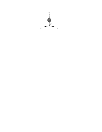
Figure 12: Contribution to the neutrino vertex function of $\gamma-Z$ self-energy. Figure 13 shows the diagrams contributing to the blob at one loop in the extended Standard Model with right-handed neutrinos.

Figure 13: $\gamma-Z$ self-energy diagrams contributing to the neutrino vertex function at one loop in the extended Standard Model with right-handed neutrinos [192, 193]. $f$ denotes a generic charged lepton ($e$, $\mu$, $\tau$) or a quark ($u$, $c$, $t$, $d$, $s$, $b$). $\chi$ is the unphysical would-be charged scalar boson. The charge of ghosts $c$ is indicated by the symbols $\oplus$ and $\ominus$.

VII.1 Neutrino electric charge

It is usually believed (see Bernstein et al. [100]) that the neutrino electric charge is exactly zero. This is true in the Standard Model, but in extensions of the Standard Model neutrinos may be millicharged particles.

In the Standard Model of $\text{SU}(2)_{L}\times\text{U}(1)_{Y}$ electroweak interactions the neutrality of neutrinos is a consequence of the quantization of electric charge [230, 377, 212, 53, 54] (see also the earlier discussions in Gross and Jackiw [275], Bardeen et al. [73], Lee and Shrock [332] and the reviews in Foot et al. [211, 213]. In the Standard Model the electric charges of the particles are related to the eigenvalue of the third component $I_{3}$ of the weak isospin $I$ and to the eigenvalue $Y$ of the hypercharge by

$$Q=I_{3}+\frac{Y}{2}.$$ (434)

The hypercharges of the fermion multiplets are fixed by the requirement of cancellation of the triangle anomalies, which is necessary for renormalizability. For each generation, let us denote with $Y_{\Phi}$, $Y_{L}$, $Y_{Q}$, $Y_{e}$, $Y_{u}$, $Y_{d}$ the hypercharges of the Higgs doublet, the left-handed lepton doublet, the left-handed quark doublet, the right-handed electron singlet, the right-handed up-quark singlet, the right-handed down-quark singlet, respectively. The electric charge can be defined in units of the charge of the Higgs field $\phi^{+}$ (see Table 1) by choosing $Y_{\Phi}=+1$. Then, the $\text{U}(1)_{Y}$ gauge invariance of the Yukawa couplings that generate the charged leptons and quarks masses requires that

$$\hbox{}Y_{e}=Y_{L}-1,$$ (435)

$$\hbox{}Y_{u}=Y_{Q}+1,$$ (436)

$$\hbox{}Y_{d}=Y_{Q}-1.$$ (437)

Taking into account that quarks have three colors, the values of $Y_{L}$ and $Y_{Q}$ are constrained by the cancellation of the $\text{SU}(2)_{L}$ triangle anomaly by

$$Y_{Q}=-Y_{L}/3.$$ (438)

Finally, the cancellation of the $\text{U}(1)_{Y}$ triangle anomaly requires that

$$0=\text{Tr}\!\left[Y^{3}\right]=2Y_{L}^{3}+6Y_{Q}^{3}-Y_{e}^{3}-3\left(Y_{u}^{3}+Y_{d}^{3}\right),$$ (439)

where the right-handed fields enter with a minus sign. Using Eqs. (435)–(438) in Eq. (439), we obtain

$$0=\text{Tr}\!\left[Y^{3}\right]=\left(Y_{L}+1\right)^{3}\quad\Longrightarrow\quad Y_{L}=-1.$$ (440)

Therefore, charge is quantized and from Eq. (434) neutrinos are exactly neutral (see also the explicit calculations in Bardeen et al. [73], Beg et al. [85], Marciano and Sirlin [363], Sakakibara [447], Lucio et al. [357, 358], Cabral-Rosetti et al. [127]).

This beautiful proof of charge quantization is spoiled by the introduction of a right-handed $\text{SU}(2)_{L}$ singlet neutrino $\nu_{R}$ in order to have a Dirac neutrino mass. Denoting with $Y_{\nu}$ the hypercharge of $\nu_{R}$, the $\text{U}(1)_{Y}$ gauge invariance of the Yukawa coupling that generates a Dirac neutrino mass requires that

$$Y_{\nu}=Y_{L}+1.$$ (441)

Then, Eq. (440) becomes

$$\text{Tr}\!\left[Y^{3}\right]=\left(Y_{L}+1\right)^{3}-\left(Y_{L}+1\right)^{3}=0.$$ (442)

Therefore, there is no $\text{U}(1)_{Y}$ triangle anomaly for any value of $Y_{L}$,a right-handed $\text{SU}(2)_{L}$ singlet neutrino $\nu_{R}$ which remains unconstrained. With the definition $Y_{\nu}=2\varepsilon$, using the relations in Eqs. (434)–(438) and (441), we obtain

$$Q_{\nu}=\hbox{} \hbox{}\varepsilon,$$ (443)

$$Q_{e}=\hbox{} \hbox{}-1+\varepsilon,$$ (444)

$$Q_{u}=\hbox{} \hbox{}2/3-\varepsilon/3,$$ (445)

$$Q_{d}=\hbox{} \hbox{}-1/3-\varepsilon/3.$$ (446)

For the proton and the neutron we have

$$Q_{p}=1-\varepsilon,\quad Q_{n}=-\varepsilon.$$ (447)

Hence, the hydrogen atom is neutral, but all the atoms with neutrons are not. Obviously, the limits on the non-neutrality of matter [364, 122] imply that the value of $\varepsilon$ must be very small. In this case, neutrinos may be electrically millicharged particles [377, 212, 53, 54] (see also the discussions in Okun et al. [400], Shrock [468]).

From Eqs. (443)–(446) one can see that the nonstandard hypercharge proportional to $\varepsilon$ is proportional to $\text{B}-\text{L}$, where B and L are the baryon and lepton numbers. With the introduction of the right-handed neutrino $\nu_{R}$ the $\text{U}(1)_{\text{B}-\text{L}}$ symmetry of the Standard Model becomes anomaly-free. Adopting a notation similar to that used for the hypercharges, in the Standard Model the $\text{U}(1)_{\text{B}-\text{L}}$ triangle anomaly is proportional to

$$\text{Tr}\!\left[(\text{B}-\text{L})^{3}\right]=\hbox{} \hbox{}2(\text{B}-\text{L})_{L}^{3}+6(\text{B}-\text{L})_{Q}^{3}-(\text{B}-\text{L})_{e}^{3}$$

$$\hbox{}-3\left((\text{B}-\text{L})_{u}^{3}+(\text{B}-\text{L})_{d}^{3}\right)$$

$$=\hbox{} \hbox{}-1.$$ (448)

Hence, in the Standard Model the $\text{U}(1)_{\text{B}-\text{L}}$ symmetry is not anomaly-free and cannot be gauged. On the other hand, with the introduction of $\nu_{R}$ which has $(\text{B}-\text{L})_{\nu}=-1$ we obtain $\text{Tr}\!\left[(\text{B}-\text{L})^{3}\right]=0$. In this case the $\text{U}(1)_{\text{B}-\text{L}}$ symmetry is anomaly-free and can be gauged. Then, there can be a mixing of the Standard Model hypercharge $Y_{\text{SM}}$ and $\text{B}-\text{L}$, which leads to the hypercharge

$$Y=Y_{\text{SM}}-2\varepsilon\left(\text{B}-\text{L}\right),$$ (449)

and the dequantized electric charges in Eqs. (443)–(446). Hence, the dequantization of the electric charge is due to the appearance of an anomaly-free $U(1)$ symmetry which can be gauged and can mix with the standard hypercharge [212, 53, 54]. The addition of an anomaly-free $U(1)$ symmetry to the symmetries of the Lagrangian is a general way to obtain charge dequantization [287].

A well-known way to recover electric charge quantization in theories with right-handed $\text{SU}(2)_{L}$ singlet neutrinos is to consider grand unified theories (GUT) in which there is no $U(1)$ symmetry [411, 231]. However, there is also the natural possibility to allow the right-handed neutrino to have a Majorana mass [53, 54]. In this case the gauge invariance of the Majorana mass term $\nu_{R}^{T}\mathcal{C}^{\dagger}\nu_{R}$ requires that $Y_{\nu}=0$ and, from Eq. (441), $Y_{L}=-1$, which gives the same charge quantization as in the Standard Model. This is consistent with the violation of the $\text{U}(1)_{\text{B}-\text{L}}$ symmetry by the Majorana mass term, which forbids the addition of the $\text{B}-\text{L}$ term to $Y_{\text{SM}}$ in Eq. (449).

Until now in this Subsection we have considered only one generations, but we know that there are three generations and the Standard Model Lagrangian has four global $\text{U}(1)$ symmetries: $\text{U}(1)_{\text{B}}$, $\text{U}(1)_{\text{L}_{e}}$, $\text{U}(1)_{\text{L}_{\mu}}$ and $\text{U}(1)_{\text{L}_{\tau}}$, associated with the conservation of the baryon number B, the electron lepton number $\text{L}_{e}$, the muon lepton number $\text{L}_{\mu}$ and the tau lepton number $\text{L}_{\tau}$. It turns out that there is an infinite number of linear combinations of these $\text{U}(1)$ symmetries which are anomaly-free and lead to electric charge dequantization in the Standard Model with three generations [210, 211, 213]. Charge quantization can be recovered by introducing right-handed neutrinos with Majorana mass terms which violate the conservation of all lepton numbers [210, 211, 213, 475].

Some approximate constraints obtained with various assumptions from reactor, accelerator and astrophysical data are listed in Tab. 4 (see also Babu and Volkas [55], Raffelt [427], Davidson et al. [161], Beringer et al. [93]).

Limit	Method	Reference
$|\mathbbm{q}_{\nu_{\tau}}|\lesssim 3\times 10^{-4}\,e$	SLAC $e^{-}$ beam dump	Davidson et al. [159]
$|\mathbbm{q}_{\nu_{\tau}}|\lesssim 4\times 10^{-4}\,e$	BEBC beam dump	Babu et al. [51]
$|\mathbbm{q}_{\nu}|\lesssim 6\times 10^{-14}\,e$	Solar cooling (plasmon decay)	Raffelt [433]
$|\mathbbm{q}_{\nu}|\lesssim 2\times 10^{-14}\,e$	Red giant cooling (plasmon decay)	Raffelt [433]
$|\mathbbm{q}_{\nu_{e}}|\lesssim 3\times 10^{-21}\,e$	Neutrality of matter	Raffelt [433]
$|\mathbbm{q}_{\nu_{e}}|\lesssim 3.7\times 10^{-12}\,e$	Nuclear reactor	Gninenko et al. [242]
$|\mathbbm{q}_{\nu_{e}}|\lesssim 1.5\times 10^{-12}\,e$	Nuclear reactor	Studenikin [489]

Table 4: Approximate limits for different neutrino effective charges. The limits on $\mathbbm{q}_{\nu}$ apply to all flavors.

The most severe experimental constraint on neutrino electric charges is that on the effective electron neutrino charge $\mathbbm{q}_{\nu_{e}}$, which can be obtained from electric charge conservation in neutron beta decay $n\to p+e^{-}+\bar{\nu}_{e}$, from the experimental limits on the non-neutrality of matter which constrain the sum of the proton and electron charges, $\mathbbm{q}_{p}+\mathbbm{q}_{e}$, and from the experimental limits on the neutron charge $\mathbbm{q}_{n}$ [427, 433]. Several experiments which measured the neutrality of matter give their results in terms of

$$\mathbbm{q}_{\text{mat}}=\frac{Z(\mathbbm{q}_{p}+\mathbbm{q}_{e})+N\mathbbm{q}_{n}}{A},$$ (450)

where $A=Z+N$ is the atomic mass of the substance under study, $Z$ is its atomic number and $N$ is its neutron number. From electric charge conservation in neutron beta decay, we have

$$\mathbbm{q}_{\nu_{e}}=\mathbbm{q}_{n}-(\mathbbm{q}_{p}+\mathbbm{q}_{e})=\frac{A}{Z}\left(\mathbbm{q}_{n}-\mathbbm{q}_{\text{mat}}\right).$$ (451)

The best recent bound on the non-neutrality of matter [122],

$$\mathbbm{q}_{\text{mat}}=(-0.1\pm 1.1)\times 10^{-21}\,e,$$ (452)

has been obtained with $\text{S}\text{F}_{6}$, which has $A=146.06$ and $Z=70$. Using the independent measurement of the charge of the free neutron [79]

$$\mathbbm{q}_{n}=(-0.4\pm 1.1)\times 10^{-21}\,e,$$ (453)

we obtain

$$\mathbbm{q}_{\nu_{e}}=(-0.6\pm 3.2)\times 10^{-21}\,e.$$ (454)

This value is compatible with the neutrality of matter limit in Tab. 4, which has been derived [427, 433] from the value of $\mathbbm{q}_{n}$ in Eq. (453) and $\mathbbm{q}_{\text{mat}}=(0.8\pm 0.8)\times 10^{-21}\,e$ [364].

It is also interesting that the effective charge of $\bar{\nu}_{e}$ can be constrained by the SN 1987A neutrino measurements taking into account that galactic and extragalactic magnetic field can lengthen the path of millicharged neutrinos and requiring that neutrinos with different energies arrive on Earth within the observed time interval of a few seconds [69]:

$$|\mathbbm{q}_{\nu_{e}}|\lesssim 3.8\times 10^{-12}\frac{(E_{\nu}/10\,\text{MeV})}{(d/10\,\text{kpc})(B/1\,\mu\text{G})}\sqrt{\frac{\Delta{t}/t}{\Delta{E_{\nu}}/E_{\nu}}},$$ (455)

considering a magnetic field $B$ acting over a distance $d$ and the corresponding time $t=d/c$. $E_{\nu}\approx 15\,\text{MeV}$ is the average neutrino energy, $\Delta{E_{\nu}}\approx E_{\nu}/2$ is the energy spread, and $\Delta{t}\approx 5\,\text{s}$ is the arrival time interval. Barbiellini and Cocconi [69] considered 2 cases:

1. An intergalactic field $B\approx 10^{-3}\,\mu\text{G}$ acting over the whole path $d\simeq 50\,\text{kpc}$, which corresponds to $t\simeq 5\times 10^{12}\,\text{s}$, gives

   $$|\mathbbm{q}_{\nu_{e}}|\lesssim 2\times 10^{-15}\,e.$$ (456)

2. An galactic field $B\approx 1\,\mu\text{G}$ acting over a distance $d\simeq 10\,\text{kpc}$, which corresponds to $t\simeq 1\times 10^{12}\,\text{s}$, gives

   $$|\mathbbm{q}_{\nu_{e}}|\lesssim 2\times 10^{-17}\,e.$$ (457)

The last two limits in Tab. 4 have been obtained [242, 489] considering the results of reactor neutrino magnetic moment experiments (see Sections IV.3 and IV.5). The differential cross section of the $\bar{\nu}_{e}$–$e^{-}$ elastic-scattering process due to a neutrino effective charge $\mathbbm{q}_{\nu_{e}}$ is given by (see Berestetskii et al. [91])

$$\left(\frac{d\sigma}{dT_{e}}\right)_{\text{charge}}\simeq 2\pi\alpha\frac{1}{m_{e}T_{e}^{2}}\mathbbm{q}_{\nu_{e}}^{2}.$$ (458)

In reactor experiments the neutrino magnetic moment is searched by considering data with $T_{e}\ll E_{\nu}$, for which the ratio of the charge cross section (458) and the magnetic moment cross section in Eq. (209), for which we consider only the dominant part proportional to $1/T_{e}$, is given by

$$R=\frac{\left(d\sigma/dT_{e}\right)_{\text{charge}}}{\left(d\sigma/dT_{e}\right)_{\text{mag}}}\simeq\frac{2m_{e}}{T_{e}}\frac{\left(\mathbbm{q}_{\nu_{e}}/e\right)^{2}}{\left(\bbmu_{\nu_{e}}/\mu_{\text{B}}\right)^{2}}$$ (459)

Considering an experiment which does not observe any effect of $\bbmu_{\nu_{e}}$ and obtains a limit on $\bbmu_{\nu_{e}}$, it is possible to obtain, following Studenikin [489], a bound on $\mathbbm{q}_{\nu_{e}}$ by demanding that the effect of $\mathbbm{q}_{\nu_{e}}$ is smaller than that of $\bbmu_{\nu_{e}}$, i.e that $R\lesssim 1$:

$$\mathbbm{q}_{\nu_{e}}^{2}\lesssim\frac{T_{e}}{2m_{e}}\left(\frac{\bbmu_{\nu_{e}}}{\mu_{\text{B}}}\right)^{2}e^{2}.$$ (460)

The last limit in Tab. 4 has been obtained from the 2012 results [82] of the GEMMA experiment, considering $T_{e}$ at the experimental threshold of $2.8\,\text{keV}$.

Let us finally note that a strong limit on a generic neutrino electric charge $\mathbbm{q}_{\nu}$ can be obtained by considering the influence of millicharged neutrinos on the rotation a magnetized star which is undergoing a core-collapse supernova explosion (the neutrino star turning mechanism, $\nu$ST) [491]. During the supernova explosion, the escaping millicharged neutrinos move along curved orbits inside the rotating magnetized star and slow down the rotation of the star. This mechanism could prevent the generation of a rapidly rotating pulsar in the supernova explosion. Imposing that the frequency shift of a forming pulsar due to the neutrino star turning mechanism is less than a typical observed frequency of $0.1\,\text{s}^{-1}$ and assuming a magnetic field of the order of $10^{14}\,\text{Gauss}$, Studenikin and Tokarev [491] obtained

$$|\mathbbm{q}_{\nu}|\lesssim 1.3\times 10^{-19}\,e.$$ (461)

Note that this limit is much stronger than the astrophysical limits in Tab. 4.

Method	Experiment	Limit [$\text{cm}^{2}$]	CL	Reference
Reactor $\bar{\nu}_{e}$-$e^{-}$	Krasnoyarsk	$|\langle{r_{\nu_{e}}^{2}}\rangle|<7.3\times 10^{-32}$	90%	Vidyakin et al. [508]
	TEXONO	$-4.2\times 10^{-32}<\langle{r_{\nu_{e}}^{2}}\rangle<6.6\times 10^{-32}$	90%	Deniz et al. [165]${}^{\text{\ref{G041}}}$
Accelerator $\nu_{e}$-$e^{-}$	LAMPF	$-7.12\times 10^{-32}<\langle{r_{\nu_{e}}^{2}}\rangle<10.88\times 10^{-32}$	90%	Allen et al. [32]
	LSND	$-5.94\times 10^{-32}<\langle{r_{\nu_{e}}^{2}}\rangle<8.28\times 10^{-32}$	90%	Auerbach et al. [47]${}^{\text{\ref{G041}}}$
Accelerator $\nu_{\mu}$-$e^{-}$	BNL-E734	$-4.22\times 10^{-32}<\langle{r_{\nu_{\mu}}^{2}}\rangle<0.48\times 10^{-32}$	90%	Ahrens et al. [14]${}^{\text{\ref{G041}}}$
	CHARM-II	$|\langle{r_{\nu_{\mu}}^{2}}\rangle|<1.2\times 10^{-32}$	90%	Vilain et al. [509]${}^{\text{\ref{G041}}}$

Table 5: Experimental limits for the electron neutrino charge radius.

VII.2 Neutrino charge radius

Even if the electric charge of a neutrino is zero, the electric form factor $\mathbbm{f}_{Q}(q^{2})$ can contain nontrivial information about the neutrino electric properties. In fact, a neutral particle can be characterized by a (real or virtual) superposition of two different charge distributions of opposite signs, which is described by a form factor $\mathbbm{f}_{Q}(q^{2})$ which is nonzero for $q^{2}\neq 0$.

The neutrino charge radius is determined by the second term in the expansion of the neutrino charge form factor $\mathbbm{f}_{Q}(q^{2})$ in series of powers of $q^{2}$:

$$\mathbbm{f}_{Q}(q^{2})=\mathbbm{f}_{Q}(0)+q^{2}\left.\frac{d\mathbbm{f}_{Q}(q^{2})}{dq^{2}}\right|_{q^{2}=0}+\ldots.$$ (462)

In the so-called “Breit frame”, in which $q_{0}=0$, the charge form factor $\mathbbm{f}_{Q}(q^{2})$ depends only on $|\vv{q}|=\sqrt{-q^{2}}$ and can be interpreted as the Fourier transform of a spherically symmetric charge distribution $\rho(r)$, with $r=|\vv{x}|$:

$$\mathbbm{f}_{Q}(q^{2})=\int\rho(r)e^{-i\vv{q}\cdot\vv{x}}d^{3}x=\int\rho(r)\frac{\sin(|\vv{q}|r)}{|\vv{q}|r}d^{3}x.$$ (463)

Deriving with respect to $q^{2}=-|\vv{q}|^{2}$, we obtain

$$\frac{d\mathbbm{f}_{Q}(q^{2})}{dq^{2}}=\int\rho(r)\frac{\sin(|\vv{q}|r)-|\vv{q}|r\cos(|\vv{q}|r)}{2q^{3}r}d^{3}x,$$ (464)

and

$$\lim_{q^{2}\to 0}\frac{d\mathbbm{f}_{Q}(q^{2})}{dq^{2}}=\int\rho(r)\frac{r^{2}}{6}d^{3}x=\frac{\langle{r}^{2}\rangle}{6}.$$ (465)

Therefore, the squared neutrino charge radius is given by

$$\langle{r}^{2}\rangle=6\,\left.\frac{d\mathbbm{f}_{Q}(q^{2})}{dq^{2}}\right|_{q^{2}=0}.$$ (466)

Note that $\langle{r}^{2}\rangle$ can be negative, because the charge density $\rho(r)$ is not a positively defined quantity.

As we have seen in Subsection III.3, massless left-handed Weyl neutrinos have the electromagnetic form factor in Eq. (167). This is the case of the Standard Model, in which in addition neutrinos have zero electric charge, $\mathbbm{f}_{Q}(0)=0$, as explained at the beginning of Subsection VII.1. Taking into account Eqs. (462) and (466), in the Standard Model the neutrino electromagnetic form factor for small values of $q^{2}$ is given by

$$\mathbbm{f}(q^{2})\simeq\left(\frac{\langle{r}^{2}\rangle}{6}-\mathbbm{a}\right)q^{2},$$ (467)

where $\mathbbm{a}$ is the anapole moment. Hence, in the Standard Model the form factor $\mathbbm{f}(q^{2})$ can be interpreted as a neutrino charge radius or as an anapole moment (or as a combination of both). In this section we consider the charge radius interpretation. The equivalence between the charge radius and anapole moment interpretations of $\mathbbm{f}(q^{2})$ is further discussed in the following Subsection VII.3.

The Standard Model theory of the neutrino charge radius has a long history, with some controversies which are shortly summarized in the following.

In one of the first studies [73], it was claimed that in the Standard Model and in the unitary gauge the neutrino charge radius is ultraviolet-divergent and so it is not a physical quantity. A direct one-loop calculation [192, 193] of proper vertices (Fig. 6) and $\gamma-Z$ self-energy (Figs. 12 and 13) contributions to the neutrino charge radius performed in a general $R_{\xi}$ gauge for a massive Dirac neutrino gave also a divergent result. However, it was shown [337], using the unitary gauge, that by including in addition to the usual terms also contributions from diagrams of the neutrino-lepton neutral-current scattering ($Z$ boson diagrams), it is possible to obtain for the neutrino charge radius a gauge-dependent but finite quantity. Later on, it was also shown [332] that in order to define the neutrino charge radius as a physical quantity one has to consider additional box diagrams and that in combination with contributions from the proper diagrams it is possible to obtain a finite and gauge-independent value for the neutrino charge radius. In this way, the neutrino electroweak radius was defined by Lucio et al. [357, 358] and an additional set of diagrams that give contribution to its value was discussed by Degrassi et al. [164]. Finally, Bernabeu et al. [95, 97, 98] introduced the neutrino electroweak radius as a physical observable. In the corresponding calculations, performed in the one-loop approximation including additional terms from the $\gamma-Z$ boson mixing and the box diagrams involving $W$ and $Z$ bosons, the following gauge-invariant result for the neutrino charge radius have been obtained:

$$\langle{r}_{\nu_{\ell}}^{2}\rangle_{\text{SM}}=\frac{G_{\text{F}}}{4\sqrt{2}\pi^{2}}\left[3-2\log\left(\frac{m_{\ell}^{2}}{m^{2}_{W}}\right)\right],$$ (468)

where $m_{W}$ and $m_{\ell}$ are the $W$ boson and lepton masses ($\ell=e,\mu,\tau$). This result, however, revived the discussion [218, 219, 409, 94] on the definition of the neutrino charge radius. Numerically, Eq. (468) gives [95, 98]

$$\hbox{}\langle{r}_{\nu_{e}}^{2}\rangle_{\text{SM}}=4.1\times 10^{-33}\,\text{cm}^{2},$$ (469)

$$\hbox{}\langle{r}_{\nu_{\mu}}^{2}\rangle_{\text{SM}}=2.4\times 10^{-33}\,\text{cm}^{2},$$ (470)

$$\hbox{}\langle{r}_{\nu_{\tau}}^{2}\rangle_{\text{SM}}=1.5\times 10^{-33}\,\text{cm}^{2}.$$ (471)

These value are of the same order of magnitude of the numerical estimation $\langle{r}_{\nu_{\ell}}^{2}\rangle\approx 10^{-33}\,\text{cm}^{2}$ obtained by Lucio et al. [358].

The effects of new physics beyond the Standard Model can contribute to the neutrino charge radius. However, Novales-Sanchez et al. [397] have shown that in the context of an effective electroweak Yang-Mills theory the anomalous $WW\gamma$ vertex contribution to the neutrino effective charge radius is smaller than about $10^{-34}\,\text{cm}^{2}$, which is one order of magnitude smaller than the Standard Model values in Eqs. (469)–(471).

The neutrino charge radius has an effect in the scattering of neutrinos with charged particles. The most useful process is the elastic scattering with electrons, which has been discussed in Subsection IV.3 in connection with the searches of neutrino magnetic moments. Since in the ultrarelativistic limit the charge form factor conserves the neutrino helicity (see Appendix C), a neutrino charge radius contributes to the weak-interaction cross section $(d\sigma/dT_{e})_{\text{SM}}$ of $\nu_{\ell}$–$e^{-}$ elastic scattering through the following shift of the vector coupling constant $g_{V}^{\nu_{\ell}}$ [255, 164, 511, 281]:

$$g_{V}^{\nu_{\ell}}\to g_{V}^{\nu_{\ell}}+\frac{2}{3}m_{W}^{2}\langle{r}_{\nu_{\ell}}^{2}\rangle\sin^{2}\theta_{W}.$$ (472)

Using this method, experiments which measure neutrino-electron elastic scattering can probe the neutrino charge radius. Some experimental results are listed in Tab. 5. In addition, Hirsch et al. [286] obtained the following 90% CL bounds on $\langle{r_{\nu_{\mu}}^{2}}\rangle$ from a reanalysis of CHARM-II [509] and CCFR [369] data:

$$-0.52\times 10^{-32}<\langle{r_{\nu_{\mu}}^{2}}\rangle<0.68\times 10^{-32}\,\text{cm}^{2}.$$ (473)

More recently, Barranco et al. [77] obtained the following 90% CL bounds on $\langle{r_{\nu_{e}}^{2}}\rangle$ from a combined fit of all available $\nu_{e}$–$e^{-}$ and $\bar{\nu}_{e}$–$e^{-}$ data:

$$-0.26\times 10^{-32}<\langle{r_{\nu_{e}}^{2}}\rangle<6.64\times 10^{-32}\,\text{cm}^{2}$$ (474)

The single photon production process $e^{+}+e^{-}\to\nu+\bar{\nu}+\gamma$ has been used to get bounds on the effective $\nu_{\tau}$ charge radius, assuming a negligible contribution of the $\nu_{e}$ and $\nu_{\mu}$ charge radii [33, 496, 286]. For Dirac neutrinos, Hirsch et al. [286] obtained

$$-5.6\times 10^{-32}<\langle{r_{\nu_{\tau}}^{2}}\rangle<6.2\times 10^{-32}\,\text{cm}^{2}.$$ (475)

Comparing the theoretical Standard Model values in Eqs. (469)–(471) with the experimental limits in Tab. 5 and those in Eqs. (473)–(475), one can see that they differ at most by one order of magnitude. Therefore, one may expect that the experimental accuracy will soon reach the value needed to probe the Standard Model predictions for the neutrino charge radii. This will be an important test of the Standard Model calculation of the neutrino charge radii. If the experimental value of a neutrino charge radius is found to be different from the Standard Model prediction in Eqs. (469)–(471) it will be necessary to clarify the precision of the theoretical calculation in order to understand if the difference is due to new physics beyond the Standard Model.

The neutrino charge radius has also some impact on astrophysical phenomena and on cosmology. The limits on the cooling of the Sun and white dwarfs due to the plasmon-decay process discussed in Subsection V.4 induced by a neutrino charge radius led Dolgov and Zeldovich [173] to estimate the respective limits $|\langle{r}_{\nu}^{2}\rangle|\lesssim 10^{-28}\,\text{cm}^{2}$ and $|\langle{r}_{\nu}^{2}\rangle|\lesssim 10^{-30}\,\text{cm}^{2}$ for all neutrino flavors. From the cooling of red giants Altherr and Salati [33] inferred the limit $|\langle{r}_{\nu}^{2}\rangle|\lesssim 4\times 10^{-31}\,\text{cm}^{2}$.

If neutrinos are Dirac particles, $e^{+}$–$e^{-}$ annihilations can produce right-handed neutrino-antineutrino pairs through the coupling induced by a neutrino charge radius. This process would affect primordial Big-Bang Nucleosynthesis and the energy release of a core-collapse supernova. From the measured ${}^{4}\text{He}$ yield in primordial Big-Bang Nucleosynthesis Grifols and Masso [259] obtained

$$|\langle{r}_{\nu}^{2}\rangle|\lesssim 7\times 10^{-33}\,\text{cm}^{2},$$ (476)

and from SN 1987A data Grifols and Masso [260] obtained

$$\langle{r}_{\nu}^{2}\rangle\lesssim 2\times 10^{-33}\,\text{cm}^{2},$$ (477)

for all neutrino flavors.

VII.3 Neutrino anapole moment

The notion of an anapole moment for a Dirac particle was introduced by Zel’dovich [532] after the discovery of parity violation. The anapole form factor was not known before because it violates P. Indeed, taking into account that

$$A_{\mu}(x)\xrightarrow{\;\text{P}\;}A^{\mu}(x_{\text{P}}),$$ (478)

P is conserved if

$$\Lambda_{\mu}(q)\xrightarrow{\;\text{P}\;}\Lambda^{\mu}(q).$$ (479)

Using the formulae in Appendix A, one can find that

$$\Lambda_{\mu}(q)\xrightarrow{\;\text{P}\;}\gamma^{0}\Lambda_{\mu}(q_{\text{P}})\gamma^{0}.$$ (480)

Using the form-factor expansion in Eq. (99), we obtain

$$\Lambda_{\mu}(q)\hbox{} \hbox{}\xrightarrow{\;\text{P}\;}\mathbbm{f}_{Q}(q^{2})\gamma^{\mu}-\mathbbm{f}_{M}(q^{2})i\sigma^{\mu\nu}q_{\nu}$$

$$\hbox{}-\mathbbm{f}_{E}(q^{2})\sigma^{\mu\nu}q_{\nu}\gamma_{5}-\mathbbm{f}_{A}(q^{2})(q^{2}\gamma^{\mu}-q^{\mu}\not{q})\gamma_{5}.$$ (481)

Hence, parity is violated by the electric and anapole moments. Since the anapole moment conserves CP (and T, as a consequence of CPT symmetry), as shown in Subsection III.1, it follows that the anapole moment violates also C.

In order to understand the physical characteristics of the anapole moment, we consider its effect in the interactions with external electromagnetic fields. From the last term in Eq. (306) one can see that the anapole moment describes an interaction with the current which generates the external electromagnetic fields.

Using the method described in Appendix E, we obtain the helicity-conserving potential

$$V_{h\to h}=-\mathbbm{a}\,h\frac{m}{E}\,s^{\mu}j_{\mu},$$ (482)

which is strongly suppressed for ultrarelativistic neutrinos. In the nonrelativistic limit, we obtain

$$V_{h\to h}^{\text{nr}}\simeq\vv{\mathbbm{a}}\cdot\vv{j},\quad\text{with}\quad\vv{\mathbbm{a}}=h\,\frac{\vv{p}}{|\vv{p}|}\,\mathbbm{a}.$$ (483)

This is the anapole moment potential that was introduced by Zel’dovich [532]. It is proportional to the longitudinal component of the current.

Considering now the helicity-flipping potential, as shown at the end of Appendix E, we obtain

$$V_{-h\to h}=\mathbbm{a}\,\frac{m}{E}\,j_{\perp},$$ (484)

where $j_{\perp}$ is the component of $\vv{j}$ orthogonal to $\vv{p}$. For ultrarelativistic neutrinos, the helicity-flipping potential is strongly suppressed, but in the nonrelativistic limit we have

$$V_{-h\to h}^{\text{nr}}\simeq\mathbbm{a}\,j_{\perp}=|\vv{\mathbbm{a}}\times\vv{j}|.$$ (485)

This potential corresponds to a classical torque [532] which rotates the spin of the particle, causing periodic changes of the helicity.

The anapole moment is a quantity which is difficult to understand, because it does not generate interactions with a free electromagnetic field, but only contact interactions with the charge and current density which generates an electromagnetic field. A classical model which can help to visualize the behavior of the anapole moment has been given by Zel’dovich [532] (see also Bukina et al. [124]). In this model the anapole is represented by a current-carrying rigid toroidal solenoid. The current generates a magnetic field only inside the toroidal solenoid. Since the solenoid is rigid, there is no external magnetic field which can act on the toroidal solenoid as a whole. The only action on the toroidal solenoid can be generated by a current which passes through the solenoid and interacts with the magnetic field inside. For example, the toroidal solenoid can be immersed in an electrolytic solution which fills also the space inside the solenoid. If a current flows through the electrolytic solution, it interacts with the magnetic field inside the solenoid and generates a torque proportional to the sine of the angle between the direction of the current and the axis of the toroid. In this model the axis of the toroid corresponds to the direction of $\vv{\mathbbm{a}}$ in Eqs. (483) and the torque corresponds to the helicity-flipping potential in Eq. (485).

The neutrino anapole moment contributes to the scattering of neutrinos with charged particles. In order to discuss its effects, it is convenient to consider strictly neutral neutrinos with $\mathbbm{f}_{Q}(0)=0$ and define a reduced charge form factor $\tilde{\mathbbm{f}}_{Q}(q^{2})$ such that

$$\mathbbm{f}_{Q}(q^{2})=q^{2}\,\tilde{\mathbbm{f}}_{Q}(q^{2}).$$ (486)

Then, from Eq. (466), apart from a factor $1/6$, the reduced charge form factor at $q^{2}=0$ is just the squared neutrino charge radius:

$$\tilde{\mathbbm{f}}_{Q}(0)=\langle{r}^{2}\rangle/6.$$ (487)

Let us now consider the charge and anapole parts of the neutrino electromagnetic vertex function in Eq. (118), which can be written as

$$\Lambda_{\mu}^{Q,A}(q)=\left(\gamma_{\mu}q^{2}-q_{\mu}\not{q}\right)\left[\tilde{\mathbbm{f}}_{Q}(q^{2})+\mathbbm{f}_{A}(q^{2})\gamma_{5}\right].$$ (488)

Since for ultrarelativistic neutrinos the effect of $\gamma_{5}$ is only a sign which depends on the helicity of the neutrino (see Eq. (603)), the phenomenology of neutrino anapole moments is similar to that of neutrino charge radii. Hence, the limits on the neutrino charge radii discussed in Subsection VII.2 apply also to the neutrino anapole moments multiplied by 6.

As we have discussed in the beginning of Subsection VII.1, in the Standard Model the neutrino electric charges are exactly zero. Hence, Eqs. (488) applies to Standard Model and can be further simplified taking into account that in the Standard Model neutrinos are described by two-component massless left-handed Weyl spinors. As discussed in Subsection III.3, the $\gamma^{5}$ in Eq. (488) becomes a minus sign, leading to

$$\Lambda_{\text{SM}\mu}^{Q,A}(q)=\left(\gamma_{\mu}q^{2}-q_{\mu}\not{q}\right)\mathbbm{f}^{\text{SM}}(q^{2}),$$ (489)

with

$$\mathbbm{f}^{\text{SM}}(q^{2})=\tilde{\mathbbm{f}}_{Q}(q^{2})-\mathbbm{f}_{A}(q^{2})\xrightarrow[q^{2}\to 0]{}\frac{\langle{r}^{2}\rangle}{6}-\mathbbm{a}.$$ (490)

These equations correspond to Eqs. (166) and (167) for $\mathbbm{f}_{Q}(0)=0$. Hence, in the Standard Model the neutrino charge radius and the anapole moment are not defined separately and one can interpret arbitrarily $\mathbbm{f}^{\text{SM}}(0)$ as a charge radius or as an anapole moment. This is the correct interpretation of the statement often found in the literature that in the Standard Model $\mathbbm{a}=-\langle{r}^{2}\rangle/6$. Therefore, the Standard Model values for the neutrino charge radii in Eqs. (468)–(471) can be interpreted also as values of the corresponding neutrino anapole moments.

Some deep insight into an interpretation of the decompositions of the vertex function (99) and the neutrino form factors can be obtained in the framework of a multipole expansions of the corresponding classical electromagnetic currents [186, 187, 188]. Since in this limit the anapole form factor does not correspond to a certain multipole distribution (that is why the term “anapole” was introduced by Zel’dovich [532]), the anapole moment has a quite intricate classical analog. Therefore, Dubovik and Kuznetsov [188], Bukina et al. [124, 125] proposed to consider the toroidal dipole moment as a characteristic of the neutrino which is more convenient and transparent than the anapole moment for the description of T-invariant interactions with nonconservation of the P and C symmetries. In this case, the electromagnetic vertex of a neutrino can be rewritten in the alternative multipole (toroidal) parameterization

$$\Lambda_{\mu}(q)=\mathbbm{f}_{Q}(q^{2})\gamma_{\mu} - \mathbbm{f}_{M}(q^{2})i\sigma_{\mu\nu}q^{\nu}+\mathbbm{f}_{E}(q^{2})\sigma_{\mu\nu}q^{\nu}\gamma_{5}$$ (491)

$$+ i\mathbbm{f}_{T}(q^{2})\epsilon_{\mu\nu\lambda\rho}P^{\nu}q^{\lambda}\gamma^{\rho},$$

where $\mathbbm{f}_{T}$ is the toroidal dipole form factor and $P=p_{i}+p_{f}$. From the following identity

$$\overline{u}_{f}(p_{f})\Bigl{\{}(m_{i}-m_{f})\sigma_{\mu\nu}q^{\nu}+\left(q^{2}\gamma_{\mu}-\not{q}q_{\mu}\right)$$

$$-i\epsilon_{\mu\nu\lambda\rho}P^{\nu}q^{\lambda}\gamma^{\rho}\gamma_{5}\Bigr{\}}\gamma_{5}u_{i}(p_{i})=0,$$ (492)

it can be seen that the toroidal and anapole moments coincide in the static limit when the masses of the initial and final neutrino states are equal to each other, $m_{i}=m_{f}$ [125], i.e. the toroidal and anapole parameterizations coincide in this case.

In some sense the toroidal parameterization has a more transparent and clear physical interpretation, because it provides a one-to-one correspondence between the multipole moments and the corresponding form factors. From the properties of each term in the expression (491) for the vertex function under C, P and T transformations, it follows that in the Majorana case only the toroidal form factor survives [532, 307] and the toroidal moment of the Dirac neutrino is half of that in the Majorana case.

In one-loop calculations [188] of the toroidal (and anapole) moment of a massive and a massless Majorana neutrino (the diagrams in Figs. 6, 12 and 13 contribute) it was shown that its value does not depend significantly on the neutrino mass (through the ratios $m^{2}_{\nu_{i}}/m^{2}_{W}$) and is of the order of

$$\mathbbm{f}_{T}(q^{2}=0)\sim e\times(10^{-33}-10^{-34})\,\text{cm}^{2},$$ (493)

depending on the values of the quark masses that propagate in the loop diagrams in Fig. 13.

Note that the toroidal form factors can contribute to the neutrino vertex function in both the diagonal and off-diagonal cases.

The toroidal (anapole) interactions of a Majorana as well as a Dirac neutrino are expected to contribute to the total cross section of neutrino elastic scattering off electrons, quarks and nuclei. Because of the fact that the toroidal (anapole) interactions contribute to the helicity preserving part of the scattering of neutrinos on electrons, quarks and nuclei, its contribution to cross sections are similar to those of the neutrino charge radius. In principle, these contributions can be probed and information about toroidal moments can be extracted in low-energy scattering experiments in the future.

Different effects of the neutrino toroidal moment are discussed in Ginzburg and Tsytovich [233], Dubovik and Kuznetsov [188], Bukina et al. [124, 125]. In particular, it has been shown that the neutrino toroidal electromagnetic interactions can produce Cherenkov radiation of neutrinos propagating in a medium.

VIII Summary and perspectives

In this review we discussed the theory and phenomenology of neutrino electromagnetic properties and interactions. We have seen that most of the theoretical and experimental research has been devoted to the study of magnetic and electric dipole moments, but there has been also some interest in the investigation of neutrino millicharges and of the charge radii and anapole moments of neutrinos.

Unfortunately, so far there is not any experimental indication in favor of neutrino electromagnetic interactions and all neutrino electromagnetic properties are known to be small, with rather stringent upper bounds obtained in laboratory experiments or from astrophysical observations.

The most accessible neutrino electromagnetic property may be the charge radius, discussed in Subsection VII.2, for which the Standard Model gives a value which is only about one order of magnitude smaller than the experimental upper bounds. A measurement of a neutrino charge radius at the level predicted by the Standard Model would be another spectacular confirmation of the Standard Model, after the recent discovery of the Higgs boson (see Ellis [202]). However, such a measurement would not give information on new physics beyond the Standard Model unless the measured value is shown to be incompatible with the Standard Model value in a high-precision experiment.

The strongest current efforts to probe the physics beyond the Standard Model by measuring neutrino electromagnetic properties is the search for a neutrino magnetic moment effect in reactor $\bar{\nu}_{e}$-$e^{-}$ scattering experiments. The current upper bounds reviewed in Subsection IV.5 are more than eight orders of magnitude larger than the prediction discussed in Subsection IV.1 of the Dirac neutrino magnetic moments in the minimal extension of the Standard Model with right-handed neutrinos. Hence, a discovery of a neutrino magnetic moment effect in reactor $\bar{\nu}_{e}$-$e^{-}$ scattering experiments would be a very exciting discovery of non-minimal new physics beyond the Standard Model.

In particular, the GEMMA-II collaboration expects to reach around the year 2017 a sensitivity to $\bbmu_{\nu_{e}}\approx 1\times 10^{-11}\mu_{\text{B}}$ in a new series of measurements at the Kalinin Nuclear Power Plant with a doubled neutrino flux obtained by reducing the distance between the reactor and the detector from 13.9 m to 10 m and by reducing the energy threshold from 2.8 keV to 1.5 keV [82, 83]. The corresponding sensitivity to the neutrino electric millicharge discussed in Subsection VII.1 will reach the level of $|\mathbbm{q}_{\nu_{e}}|\approx 3.7\times 10^{-13}\,e$ [489].

There is also a GEMMA-III project to further lower the energy threshold to about 350 eV, which may allow the experimental collaboration to reach a sensitivity of $\bbmu_{\nu_{e}}\approx 9\times 10^{-12}\mu_{\text{B}}$. The corresponding sensitivity to neutrino millicharge will be $|\mathbbm{q}_{\nu_{e}}|\approx 1.8\times 10^{-13}\,e$ [489].

An interesting possibility for exploring very small values of $\bbmu_{\nu_{e}}$ in $\bar{\nu}_{e}$-$e^{-}$ scattering experiments has been proposed by Bernabeu et al. [96] on the basis of the observation [463] that “dynamical zeros” induced by a destructive interference between the left-handed and right-handed chiral couplings of the electron in the charged and neutral-current amplitudes appear in the Standard Model contribution to the scattering cross section. It may be possible to enhance the sensitivity of an experiment to $\bbmu_{\nu_{e}}$ by selecting recoil electrons contained in a forward narrow cone corresponding to a dynamical zero (see Eq. (203)).

In the future experimental searches of neutrino electromagnetic properties may be performed also with new neutrino sources, as a tritium source [370], a low-energy beta-beam [370, 247], a stopped-pion neutrino source [459], or a neutrino factory [247]. Recently Coloma et al. [147] proposed to improve the existing limit on the electron neutrino magnetic moment with a megacurie ${}^{51}\text{Cr}$ neutrino source and a large liquid Xenon detector.

Neutrino electromagnetic interactions could have important effects in astrophysical environments and in the evolution of the Universe and the current rapid advances of astrophysical and cosmological observations may lead soon to the exciting discovery of nonstandard neutrino electromagnetic properties. In particular, future high-precision observations of supernova neutrino fluxes may reveal the effects of collective spin-flavor oscillations due to Majorana transition magnetic moments as small as $10^{-21}\,\mu_{\text{B}}$ [248, 249].

Let us finally emphasize the importance of pursuing the experimental and theoretical studies of electromagnetic neutrino interactions, which could open a powerful window to new physics beyond the Standard Model.

Appendix A Conventions, useful constants and formulae

In this Appendix we clarify the conventions and notation used in the paper and we list some useful physical constants and formulae.

We use natural units in which $c=\hbar=1$, where $c$ is the velocity of light and $\hbar$ is the reduced Planck constant.

The values of the following physical constants are taken from Beringer et al. [93].

Avogadro number:

$$N_{\text{A}}=6.022\,141\,29\,(27)\times 10^{23}\,\text{mol}^{-1}.$$ (494)

Bohr magneton ($$\mu_{\text{B}}\equiv e/2m_{e}$$):

$$\mu_{\text{B}}=5.788\,381\,8066\,(38)\times 10^{-15}\,\text{MeV}\,\text{G}^{-1}$$

$$\phantom{\mu_{\text{B}}}\simeq 0.296\,\text{MeV}^{-1}.$$ (495)

Electron mass:

$$m_{e}=0.510\,998\,928\,(11)\,\text{MeV}.$$ (496)

Conversion constant:

$$\hbar c=1.973\,269\,718\,(44)\times 10^{-5}\,\text{eV}\,\text{cm}.$$ (497)

Light velocity:

$$c=299\,792\,458\,\text{m}\,\text{s}^{-1}.$$ (498)

Fermi constant:

$$G_{\text{F}}=1.166\,378\,7\,(6)\times 10^{-5}\,\text{GeV}^{-2}.$$ (499)

Fine-structure constant ($$\alpha\equiv e^{2}/4\pi Q^{2}=0$$) at :

$$\alpha^{-1}=137.035\,999\,074\,(44).$$ (500)

Neutron mass:

$$m_{n}=939.565\,379\,(21)\,\text{MeV}.$$ (501)

Proton mass:

$$m_{p}=938.272\,046\,(21)\,\text{MeV}.$$ (502)

Muon mass:

$$m_{\mu}=105.658\,3715\,(35)\,\text{MeV}.$$ (503)

Planck constant, reduced:

$$\hbar=6.582\,119\,28\,(15)\times 10^{-22}\,\text{MeV}\,\text{s}.$$ (504)

Tau mass:

$$m_{\tau}=1776.82\,(16)\,\text{MeV}.$$ (505)

Weak mixing angle (on-shell: $$\sin^{2}\theta_{W}\equiv 1-m_{W}^{2}/m_{Z}^{2}$$):

$$\sin^{2}\theta_{W}=0.222\,95\,(28).$$ (506)

For Dirac $\gamma$ matrices and related quantities we use the notation and conventions in Giunti and Kim [234]. Curly and square brackets denote, respectively, anticommutator and commutator. For a four-vector $p^{\mu}$ we use the standard notation $\not{p}\equiv p^{\mu}\gamma_{\mu}$, with the metric tensor $g^{\mu\nu}=g_{\mu\nu}=\text{diag}(1,-1,-1,-1)$ and $p^{\mu}=(p^{0},p^{1},p^{2},p^{3})=(p^{0},\vv{p})$.

Dirac $\gamma$ matrices:

$$\hbox{}\{\gamma^{\mu},\gamma^{\nu}\}=2\,g^{\mu\nu},$$ (507)

$$\hbox{}\gamma^{0}\,\gamma^{\mu}\,\gamma^{0}={\gamma^{\mu}}^{\dagger}=\gamma_{\mu}.$$ (508)

Definition and properties of $\gamma^{5}$:

$$\hbox{}\gamma^{5}\equiv i\,\gamma^{0}\,\gamma^{1}\,\gamma^{2}\,\gamma^{3}=\gamma_{5},$$ (509)

$$\hbox{}\left\{\gamma^{5},\gamma^{\mu}\right\}=0,$$ (510)

$$\hbox{}\left(\gamma^{5}\right)^{2}=\openone,$$ (511)

$$\hbox{}\left(\gamma^{5}\right)^{\dagger}=\gamma^{5},$$ (512)

$$\hbox{}\gamma^{\mu}\,\gamma^{5}=\frac{i}{6}\,\epsilon^{\mu\nu\rho\sigma}\,\gamma_{\nu}\,\gamma_{\rho}\,\gamma_{\sigma}.$$ (513)

Left-handed and right-handed chiral projectors:

$$P_{L}=\frac{1-\gamma^{5}}{2},\qquad P_{R}=\frac{1+\gamma^{5}}{2}.$$ (514)

Chiral decomposition of a Dirac field $\psi$:

$$\psi=P_{L}\psi+P_{R}\psi=\psi_{L}+\psi_{R}.$$ (515)

Definition and properties of $\sigma^{\mu\nu}$:

$$\hbox{}\sigma^{\mu\nu}\equiv\frac{i}{2}\,\left[\gamma^{\mu},\gamma^{\nu}\right]=i\,\gamma^{\mu}\,\gamma^{\nu}-i\,g^{\mu\nu},$$ (516)

$$\hbox{}\left[\gamma^{5}\,,\,\sigma^{\mu\nu}\right]=0,$$ (517)

$$\hbox{}\gamma^{0}\,\sigma^{\mu\nu}\,\gamma^{0}=(\sigma^{\mu\nu})^{\dagger}=\sigma_{\mu\nu},$$ (518)

$$\hbox{}\epsilon^{\mu\nu\alpha\beta}\sigma_{\alpha\beta}=-2i\sigma^{\mu\nu}\gamma^{5},$$ (519)

$$\hbox{}\epsilon^{\mu\nu\alpha\beta}\gamma_{\nu}=i\left(g^{\mu\alpha}g^{\nu\beta}-g^{\mu\beta}g^{\nu\alpha}\right)\gamma_{\nu}\gamma^{5}-\gamma^{\mu}\sigma^{\alpha\beta}\gamma^{5}.$$ (520)

Definition and properties of $\vv{\Sigma}$:

$$\hbox{}\Sigma^{k}\equiv\frac{1}{2}\sum_{j,l}\epsilon^{kjl}\,\sigma^{jl}=\gamma^{0}\,\gamma^{k}\,\gamma^{5},$$ (521)

$$\hbox{}[\Sigma^{k},\Sigma^{j}]=2\,i\sum_{l}\epsilon^{kjl}\,\Sigma^{l},$$ (522)

$$\hbox{}\{\Sigma^{k},\Sigma^{j}\}=2\,\delta^{kj},$$ (523)

$$\hbox{}(\Sigma^{k})^{\dagger}=\Sigma^{k},$$ (524)

$$\hbox{}[\Sigma^{k},\gamma^{0}]=[\Sigma^{k},\gamma^{5}]=0,$$ (525)

$$\hbox{}[\Sigma^{k},\gamma^{j}]=2i\sum_{\ell}\epsilon^{kj\ell}\,\gamma^{\ell}.$$ (526)

Charge-conjugation matrix:

$$\hbox{}\mathcal{C}\,\gamma_{\mu}^{T}\,\mathcal{C}^{-1}=-\gamma_{\mu},$$ (527)

$$\hbox{}\mathcal{C}^{\dagger}=\mathcal{C}^{-1},$$ (528)

$$\hbox{}\mathcal{C}^{T}=-\mathcal{C}.$$ (529)

$$\hbox{}\mathcal{C}\,(\gamma^{5})^{T}\,\mathcal{C}^{-1}=\gamma^{5},$$ (530)

$$\hbox{}\mathcal{C}\,(\sigma^{\mu\nu})^{T}\,\mathcal{C}^{-1}=-\sigma^{\mu\nu}.$$ (531)

Traces of products of $\gamma$ matrices:

$$\hbox{}\text{Tr}\!\left[\gamma^{\alpha}\,\gamma^{\beta}\right]=4\,g^{\alpha\beta},$$ (532)

$$\hbox{}\text{Tr}\!\big{[}\gamma^{\alpha}\,\gamma^{\beta}\,\gamma^{\rho}\,\gamma^{\sigma}\big{]}=4(g^{\alpha\beta}g^{\rho\sigma}-g^{\alpha\rho}g^{\beta\sigma}+g^{\alpha\sigma}g^{\beta\rho}),$$ (533)

$$\hbox{}\text{Tr}\!\left[\gamma^{\alpha}\,\gamma^{\beta}\,\gamma^{\rho}\,\gamma^{\sigma}\,\gamma^{5}\right]=-4\,i\,\epsilon^{\alpha\beta\rho\sigma}.$$ (534)

The $\gamma$ matrices are traceless. The trace of a product of an odd number of $\gamma$ matrices is zero. $\text{Tr}\!\left[\gamma^{5}\right]=\text{Tr}\!\left[\gamma^{\alpha}\,\gamma^{\beta}\,\gamma^{5}\right]=0$.

Four-momentum and helicity eigenstate spinors:

$$\hbox{}(\not{p}-m)\,u^{(h)}(p)=0,$$ (535)

$$\hbox{}(\not{p}+m)\,v^{(h)}(p)=0.$$ (536)

Normalization:

$$\overline{u^{(h)}}(p)\,u^{(h^{\prime})}(p)=2\,m\,\delta_{hh^{\prime}},$$ (537)

$$\overline{v^{(h)}}(p)\,v^{(h^{\prime})}(p)=-2\,m\,\delta_{hh^{\prime}},$$ (538)

Charge-conjugation relation:

$$u^{(h)}(p)=\mathcal{C}\,\overline{v^{(h)}}^{T}(p)$$ (539)

$$v^{(h)}(p)=\mathcal{C}\,\overline{u^{(h)}}^{T}(p).$$ (540)

Energy-projection matrices:

$$\hbox{}\Lambda_{+}(p)=\frac{m+\not{p}}{2m}=\sum_{h=\pm 1}\frac{u^{(h)}(p)\,\overline{u^{(h)}}(p)}{2m},$$ (541)

$$\hbox{}\Lambda_{-}(p)=\frac{m-\not{p}}{2m}=-\sum_{h=\pm 1}\frac{v^{(h)}(p)\,\overline{v^{(h)}}(p)}{2m}.$$ (542)

Helicity-projection matrices ($[P_{h},\Lambda_{\pm}(p)]=0$):

$$P_{h}=\frac{1+h\,\gamma^{5}\,\not{s}}{2},$$ (543)

for $h=+1$ (right-handed) and $h=-1$ (left-handed), with the polarization four-vector

$$s^{\mu}=\left(\frac{|\vv{p}|}{m}\,,\,\frac{E}{m}\,\frac{\vv{p}}{|\vv{p}|}\right),\quad s^{2}=-1,\quad s\cdot p=0.$$ (544)

The helicity eigenstate spinors satisfy

$$\hbox{}P_{h^{\prime}}u^{(h)}(p)=\frac{1}{2}\left(1+h^{\prime}\frac{\vv{p}\cdot\vv{\Sigma}}{|\vv{p}|}\right)u^{(h)}(p)=\delta_{h^{\prime}h}u^{(h)}(p),$$ (545)

$$\hbox{}P_{h^{\prime}}v^{(h)}(p)=\frac{1}{2}\left(1-h^{\prime}\frac{\vv{p}\cdot\vv{\Sigma}}{|\vv{p}|}\right)v^{(h)}(p)=\delta_{h^{\prime}h}v^{(h)}(p).$$ (546)

Moreover, since $\gamma^{0}P_{h}^{\dagger}\gamma^{0}=P_{h}$, we also have

$$\overline{u^{(h)}}(p)P_{h^{\prime}}=\delta_{h^{\prime}h}\overline{u^{(h)}}(p),\quad\overline{v^{(h)}}(p)P_{h^{\prime}}=\delta_{h^{\prime}h}\overline{v^{(h)}}(p).$$ (547)

Fourier expansion of a free Dirac field $\psi(x)$ (with $p^{0}=E=\sqrt{\vv{p}^{2}+m^{2}}$):

$$\psi(x)=\int\frac{\text{d}^{3}p}{(2\pi)^{3}\,2E}\hbox{} \hbox{}\sum_{h=\pm 1}\bigg{[}a^{(h)}(p)\,u^{(h)}(p)\,e^{-ip{\cdot}x}$$

$$\hbox{}+b^{(h)\dagger}(p)\,v^{(h)}(p)\,e^{ip{\cdot}x}\bigg{]}.$$ (548)

The operators $a^{(h)}(p)$, $a^{(h)\dagger}(p)$, $b^{(h)}(p)$, $b^{(h)\dagger}(p)$ anticommute, except for

$$\{a^{(h)}(p),a^{(h^{\prime})\dagger}(p^{\prime})\}=\hbox{} \hbox{}\{b^{(h)}(p),b^{(h^{\prime})\dagger}(p^{\prime})\}$$

$$=\hbox{} \hbox{}(2\pi)^{3}\,2E\,\delta^{3}(\vv{p}-\vv{p}^{\prime})\,\delta_{hh^{\prime}}.$$ (549)

States describing a fermion $\mathfrak{f}$ and an antifermion $\bar{\mathfrak{f}}$ with four-momentum $p$ and helicity $h$ ($|0\rangle$ is the vacuum, such that $a^{(h)}(p)|0\rangle=0$, $b^{(h)}(p)|0\rangle=0$ and $\langle 0|0\rangle=1$; $V$ is the total volume):

$$|\mathfrak{f}(p,h)\rangle=a^{(h)\dagger}(p)\,|0\rangle,\quad|\bar{\mathfrak{f}}(p,h)\rangle=b^{(h)\dagger}(p)\,|0\rangle,$$ (550)

$$\langle\mathfrak{f}(p,h)|\mathfrak{f}(p,h^{\prime})\rangle=\langle\bar{\mathfrak{f}}(p,h)|\bar{\mathfrak{f}}(p,h^{\prime})\rangle=2E\,V\,\delta_{hh^{\prime}}.$$ (551)

The Majorana condition (24) leads to the following Fourier expansion of a free Majorana field:

$$\psi(x)=\int\frac{\text{d}^{3}p}{(2\pi)^{3}\,2E}\hbox{} \hbox{}\sum_{h=\pm 1}\bigg{[}a^{(h)}(p)\,u^{(h)}(p)\,e^{-ip{\cdot}x}$$

$$\hbox{}+a^{(h)\dagger}(p)\,v^{(h)}(p)\,e^{ip{\cdot}x}\bigg{]}.$$ (552)

Gordon identities:

$$\hbox{}\overline{u_{f}}(p_{f})i\sigma^{\alpha\beta}(p_{f}-p_{i})_{\beta}u_{i}(p_{i})$$

$$\hbox{}=\overline{u_{f}}(p_{f})\left[\left(m_{f}+m_{i}\right)\gamma^{\alpha}-(p_{f}+p_{i})^{\alpha}\right]u_{i}(p_{i}),$$ (553)

$$\hbox{}\overline{u_{f}}(p_{f})i\sigma^{\alpha\beta}(p_{f}+p_{i})_{\beta}u_{i}(p_{i})$$

$$\hbox{}=\overline{u_{f}}(p_{f})\left[\left(m_{f}-m_{i}\right)\gamma^{\alpha}-(p_{f}-p_{i})^{\alpha}\right]u_{i}(p_{i}),$$ (554)

$$\hbox{}\overline{u_{f}}(p_{f})i\sigma^{\alpha\beta}(p_{f}-p_{i})_{\beta}\gamma^{5}u_{i}(p_{i})$$

$$\hbox{}=\overline{u_{f}}(p_{f})\left[\left(m_{f}-m_{i}\right)\gamma^{\alpha}-(p_{f}+p_{i})^{\alpha}\right]\gamma^{5}u_{i}(p_{i}),$$ (555)

$$\hbox{}\overline{u_{f}}(p_{f})i\sigma^{\alpha\beta}(p_{f}+p_{i})_{\beta}\gamma^{5}u_{i}(p_{i})$$

$$\hbox{}=\overline{u_{f}}(p_{f})\left[\left(m_{f}+m_{i}\right)\gamma^{\alpha}-(p_{f}-p_{i})^{\alpha}\right]\gamma^{5}u_{i}(p_{i}).$$ (556)

C, P, CP, T and CPT active transformations of a fermionic field $\psi(x)$ ($x^{\mu}_{\text{P}}=x_{\mu}$ and $x^{\mu}_{\text{T}}=-x_{\mu}$):

$$\mathsf{U}_{\text{C}}\psi(x)\mathsf{U}_{\text{C}}^{\dagger}=\hbox{} \hbox{}\xi^{\text{C}}\mathcal{C}\overline{\psi}^{T}(x),$$ (557)

$$\mathsf{U}_{\text{P}}\psi(x)\mathsf{U}_{\text{P}}^{\dagger}=\hbox{} \hbox{}\xi^{\text{P}}\gamma^{0}\psi(x_{\text{P}}),$$ (558)

$$\mathsf{U}_{\text{CP}}\psi(x)\mathsf{U}_{\text{CP}}^{\dagger}=\hbox{} \hbox{}\xi^{\text{CP}}\gamma^{0}\mathcal{C}\overline{\psi}^{T}(x_{\text{P}}),$$ (559)

$$\mathsf{U}_{\text{T}}\psi(x)\mathsf{U}_{\text{T}}^{\dagger}=\hbox{} \hbox{}\xi^{\text{T}}\mathcal{C}^{\dagger}\gamma^{5}\psi(x_{\text{T}}),$$ (560)

$$\mathsf{U}_{\text{CPT}}\psi(x)\mathsf{U}_{\text{CPT}}^{\dagger}=\hbox{} \hbox{}\xi^{\text{CPT}}\left[\psi^{\dagger}(-x)\gamma^{5}\right]^{T}.$$ (561)

Here $\xi^{\text{C}}$, $\xi^{\text{P}}$, $\xi^{\text{CP}}$, $\xi^{\text{T}}$, $\xi^{\text{CPT}}$ are phases such that $\xi^{\text{CP}}=\xi^{\text{C}}\xi^{\text{P}}$, $\xi^{\text{T}}=\pm\xi^{\text{CP}}\,\text{or}\,\pm i\xi^{\text{CP}}$, and $\xi^{\text{CPT}}=\xi^{\text{T}}{\xi^{\text{CP}}}^{*}=\pm 1\,\text{or}\,\pm i$. The operators $\mathsf{U}_{\text{C}}$, $\mathsf{U}_{\text{P}}$ and $\mathsf{U}_{\text{CP}}$ are unitary, whereas the operators $\mathsf{U}_{\text{T}}$ and $\mathsf{U}_{\text{CPT}}$ are antiunitary. An antiunitary operator $\mathsf{U}$ satisfies the standard relation $\mathsf{U}^{\dagger}=\mathsf{U}^{-1}$ of unitary operators, but is antilinear, i.e. for a real number $z$

$$\mathsf{U}z\mathsf{U}^{\dagger}=z^{*},$$ (562)

and if $|p^{\prime}\rangle=\mathsf{U}|p^{\prime}\rangle$ we have

$$\langle p^{\prime}_{1}|p^{\prime}_{2}\rangle=\langle p_{1}|\mathsf{U}^{\dagger}\mathsf{U}|p_{2}\rangle^{*}=\langle p_{2}|p_{1}\rangle.$$ (563)

Maxwell equations in the International System of Units (SI):

$$\partial_{\mu}F^{\mu\nu}(x)=j^{\nu}(x),\qquad\partial_{\mu}\widetilde{F}^{\mu\nu}(x)=0,$$ (564)

where $j^{\mu}(x)=(\rho(x),\vv{j}(x))$ is the four-vector of the charge and current density and

$$\hbox{}F^{\mu\nu}(x)=\partial^{\mu}A^{\nu}(x)-\partial^{\nu}A^{\mu}(x),$$ (565)

$$\hbox{}\widetilde{F}^{\mu\nu}(x)\equiv\frac{1}{2}\epsilon^{\mu\nu\rho\sigma}F_{\rho\sigma}(x),$$ (566)

where $A^{\mu}(x)$ is the electromagnetic field. The electromagnetic tensor $F^{\mu\nu}(x)$ contains the physical electric field $\vv{E}(x)$ and magnetic field $\vv{B}(x)$:

$$E^{k}(x)=F^{k0}(x),\qquad B^{k}(x)=-\frac{1}{2}\sum_{j,\ell}\epsilon^{kj\ell}F^{j\ell}(x).$$ (567)

The Maxwell equations for the electromagnetic field are ($\square\equiv\partial_{\mu}\partial^{\mu}$):

$$\square A^{\mu}(x)-\partial^{\mu}\partial_{\nu}A^{\nu}(x)=j^{\mu}(x).$$ (568)

Appendix B Decomposition of $\Lambda_{\mu}$

In this Appendix (see also Nowakowski et al. [398]) we derive the general expression of $\Lambda_{\mu}(p_{\text{i}},p_{\text{f}})$ in the matrix element

$$\langle\nu_{f}(p_{\text{f}})|j_{\mu}^{(\nu)}(0)|\nu_{i}(p_{\text{i}})\rangle=\overline{u_{f}}(p_{\text{f}})\Lambda_{\mu}(p_{\text{i}},p_{\text{f}})u_{i}(p_{\text{i}}).$$ (569)

The initial and final massive neutrinos can be different, but since they are considered as free particles they are on shell, with four-momenta $p_{i}$ and $p_{f}$ such that

$$p_{i}^{2}=m_{i}^{2},\qquad p_{f}^{2}=m_{f}^{2},$$ (570)

We use the notation

$$q\equiv p_{i}-p_{f},\qquad t\equiv p_{i}+p_{f},$$ (571)

for which we have

$$q^{2}+t^{2}=2\left(m_{f}^{2}+m_{i}^{2}\right),\qquad q\cdot t=m_{i}^{2}-m_{f}^{2}.$$ (572)

In general, $\Lambda^{\mu}(q,t)$ can be expanded as a linear combination of the 16 matrices

$$\openone,\qquad\gamma^{\mu},\qquad\sigma^{\mu\nu}\equiv\frac{i}{2}\,[\gamma^{\mu},\gamma^{\nu}],\qquad\gamma^{\mu}\gamma^{5},\qquad\gamma^{5},$$ (573)

which form a basis in the vectorial space of $4\times 4$ matrices (see Giunti and Kim [234]). Since $\Lambda^{\mu}(q,t)$ carries a Lorentz index, the coefficients of this expansion can depend on the available tensors: the four-vectors $q^{\mu}$, $t^{\mu}$, the Lorentz-invariant metric tensor $g^{\mu\nu}$ and the Lorentz-invariant antisymmetric tensor $\epsilon^{\mu\nu\alpha\beta}$. Let us consider separately each term of the expansion:

1. The $\openone$ term is a linear combination of the set

   $$S(\openone)=\left\{q^{\mu}\openone,\,t^{\mu}\openone\right\}.$$ (574)

2. The $\gamma^{\mu}$ term is a linear combination of the set

   $$S(\gamma^{\mu})=\left\{\gamma^{\mu},\,q^{\mu}\not{q},\,q^{\mu}\not{t},\,t^{\mu}\not{q},\,t^{\mu}\not{t},\,\epsilon^{\mu\nu\alpha\beta}\gamma_{\nu}q_{\alpha}t_{\beta}\right\}.$$ (575)

3. The $\sigma^{\mu\nu}$ term is a linear combination of the set

   $$S(\sigma^{\mu\nu})=\hbox{} \hbox{}\left\{\sigma^{\mu\nu}q_{\nu},\,\sigma^{\mu\nu}t_{\nu},\,q^{\mu}\sigma^{\alpha\beta}q_{\alpha}t_{\beta},\,t^{\mu}\sigma^{\alpha\beta}q_{\alpha}t_{\beta},\,\right.$$

   $$\hbox{}\phantom{\{}\left.\epsilon^{\mu\nu\alpha\beta}q_{\nu}\sigma_{\alpha\beta},\,\epsilon^{\mu\nu\alpha\beta}t_{\nu}\sigma_{\alpha\beta},\,\right.$$

   $$\hbox{}\phantom{\{}\left.\epsilon^{\mu\nu\alpha\beta}\sigma_{\nu\rho}q_{\alpha}t_{\beta}q^{\rho},\,\epsilon^{\mu\nu\alpha\beta}\sigma_{\nu\rho}q_{\alpha}t_{\beta}t^{\rho}\right\}.$$ (576)

4. The $\gamma^{\mu}\gamma^{5}$ term is a linear combination of the set

   $$S(\gamma^{\mu}\gamma^{5})=\hbox{} \hbox{}\left\{\gamma^{\mu}\gamma^{5},\,q^{\mu}\not{q}\gamma^{5},\,q^{\mu}\not{t}\gamma^{5},\,t^{\mu}\not{q}\gamma^{5},\,t^{\mu}\not{t}\gamma^{5},\,\right.$$

   $$\hbox{}\phantom{\{}\left.\epsilon^{\mu\nu\alpha\beta}\gamma_{\nu}q_{\alpha}t_{\beta}\gamma^{5}\right\}.$$ (577)

5. The $\gamma^{5}$ term is a linear combination of the set

   $$S(\gamma^{5})=\left\{q^{\mu}\gamma^{5},\,t^{\mu}\gamma^{5}\right\}.$$ (578)

Several elements of the sets (574)–(578) can be expressed as linear combinations of others, leading to only six independent elements. It is convenient to choose the set of six independent elements as

$$q^{\mu}\openone,\quad q^{\mu}\gamma^{5},\quad\gamma^{\mu},\quad\gamma^{\mu}\gamma^{5},\quad\sigma^{\mu\nu}q_{\nu},\quad\epsilon^{\mu\nu\alpha\beta}q_{\nu}\sigma_{\alpha\beta}.$$ (579)

We express all the elements in the sets (574)–(578) in terms of the six elements in the set (579) using the equations in Appendix A as follows (above each arrow we indicate the main equations used in the decomposition):

1. From $S(\openone)$:

   $$t^{\mu}\openone\xrightarrow{\text{(\ref{I072})}}\left\{\gamma^{\mu},\,\sigma^{\mu\nu}q_{\nu}\right\}.$$ (580)

2. From $S(\gamma^{\mu})$:

   $$q^{\mu}\not{q}\hbox{} \hbox{}\xrightarrow{\text{(\ref{I043})}}\left\{q^{\mu}\openone\right\},$$ (581)

   $$q^{\mu}\not{t}\hbox{} \hbox{}\xrightarrow{\text{(\ref{I043})}}\left\{q^{\mu}\openone\right\},$$ (582)

   $$t^{\mu}\not{q}\hbox{} \hbox{}\xrightarrow{\text{(\ref{I072})}}\left\{\gamma^{\mu},\,\sigma^{\mu\nu}q_{\nu}\right\},$$ (583)

   $$t^{\mu}\not{t}\hbox{} \hbox{}\xrightarrow{\text{(\ref{I072})}}\left\{\gamma^{\mu},\,\sigma^{\mu\nu}q_{\nu}\right\},$$ (584)

   $$\epsilon^{\mu\nu\alpha\beta}\gamma_{\nu}q_{\alpha}t_{\beta}\hbox{} \hbox{}\xrightarrow{\text{(\ref{I028})+(\ref{I074})}}\left\{q^{\mu}\gamma^{5},\,\gamma^{\mu}\gamma^{5},\,\epsilon^{\mu\nu\alpha\beta}q_{\nu}\sigma_{\alpha\beta}\right\}.$$ (585)

3. From $S(\sigma^{\mu\nu})$:

   $$\sigma^{\mu\nu}t_{\nu}\hbox{} \hbox{}\xrightarrow{\text{(\ref{I073})}}\left\{q^{\mu}\openone,\,\gamma^{\mu}\right\},$$ (586)

   $$q^{\mu}\sigma^{\alpha\beta}q_{\alpha}t_{\beta}\hbox{} \hbox{}\xrightarrow{\text{(\ref{I073})}}\left\{q^{\mu}\openone\right\},$$ (587)

   $$t^{\mu}\sigma^{\alpha\beta}q_{\alpha}t_{\beta}\hbox{} \hbox{}\xrightarrow{\text{(\ref{I072})}}\left\{\gamma^{\mu},\,\sigma^{\mu\nu}q_{\nu}\right\},$$ (588)

   $$\epsilon^{\mu\nu\alpha\beta}t_{\nu}\sigma_{\alpha\beta}\hbox{} \hbox{}\xrightarrow{\text{(\ref{I075})}}\left\{q^{\mu}\gamma^{5},\,\gamma^{\mu}\gamma^{5}\right\},$$ (589)

   $$\epsilon^{\mu\nu\alpha\beta}\sigma_{\nu\rho}q_{\alpha}t_{\beta}q^{\rho}\hbox{} \hbox{}\xrightarrow{\text{(\ref{I028})+(\ref{I074})}}\left\{q^{\mu}\gamma^{5},\,\gamma^{\mu}\gamma^{5},\,\epsilon^{\mu\nu\alpha\beta}q_{\nu}\sigma_{\alpha\beta}\right\},$$ (590)

   $$\epsilon^{\mu\nu\alpha\beta}\sigma_{\nu\rho}q_{\alpha}t_{\beta}t^{\rho}\hbox{} \hbox{}\xrightarrow{\text{(\ref{I028})+(\ref{I074})}}\left\{q^{\mu}\gamma^{5},\,\gamma^{\mu}\gamma^{5},\,\epsilon^{\mu\nu\alpha\beta}q_{\nu}\sigma_{\alpha\beta}\right\}.$$ (591)

4. From $S(\gamma^{\mu}\gamma^{5})$:

   $$q^{\mu}\not{q}\gamma^{5}\hbox{} \hbox{}\xrightarrow{\text{(\ref{I043})}}\left\{q^{\mu}\gamma^{5}\right\},$$ (592)

   $$q^{\mu}\not{t}\gamma^{5}\hbox{} \hbox{}\xrightarrow{\text{(\ref{I043})}}\left\{q^{\mu}\gamma^{5}\right\},$$ (593)

   $$t^{\mu}\not{q}\gamma^{5}\hbox{} \hbox{}\xrightarrow{\text{(\ref{I074})}}\left\{\gamma^{\mu}\gamma^{5},\,\epsilon^{\mu\nu\alpha\beta}q_{\nu}\sigma_{\alpha\beta}\right\},$$ (594)

   $$t^{\mu}\not{t}\gamma^{5}\hbox{} \hbox{}\xrightarrow{\text{(\ref{I074})}}\left\{\gamma^{\mu}\gamma^{5},\,\epsilon^{\mu\nu\alpha\beta}q_{\nu}\sigma_{\alpha\beta}\right\},$$ (595)

   $$\epsilon^{\mu\nu\alpha\beta}\gamma_{\nu}q_{\alpha}t_{\beta}\gamma^{5}\hbox{} \hbox{}\xrightarrow{\text{(\ref{I028})+(\ref{I072})}}\left\{q^{\mu}\openone,\,\gamma^{\mu},\,\sigma^{\mu\nu}q_{\nu}\right\}.$$ (596)

5. From $S(\gamma^{5})$:

   $$t^{\mu}\gamma^{5}\xrightarrow{\text{(\ref{I074})}}\left\{\gamma^{\mu}\gamma^{5},\,\epsilon^{\mu\nu\alpha\beta}q_{\nu}\sigma_{\alpha\beta}\right\}.$$ (597)

Appendix C Helicity and chirality

In this Appendix we derive the relation between helicity and chirality for ultrarelativistic neutrinos and the corresponding helicity conservation properties of the different terms of the general expansion of $\Lambda_{\mu}^{fi}(q)$ in Eq. (116), taking into account that $\Lambda_{\mu}^{fi}(q)$ is sandwiched between $u$-spinors in the case of neutrinos (Eq. (109)) or between $v$-spinors in the case of antineutrinos (Eq. (126)).

With the help of Eqs. (535) and (536) and using the definition (544) of the polarization four-vector $s^{\mu}$, one can find that

$$\hbox{}\not{s}\,u(p)=\left(-\frac{m}{|\vv{p}|}\gamma^{0}+\frac{E}{|\vv{p}|}\right)u(p),$$ (598)

$$\hbox{}\not{s}\,v(p)=\left(-\frac{m}{|\vv{p}|}\gamma^{0}-\frac{E}{|\vv{p}|}\right)v(p).$$ (599)

Therefore, in the ultrarelativistic limit $m\ll E$ we have

$$\not{s}\,u(p)\simeq u(p)\quad\text{and}\quad\not{s}\,v(p)\simeq-v(p),$$ (600)

and the helicity-projection matrices in Eq. (543) have the same effect as the chirality projection matrices in Eq. (514):

$$\hbox{}P_{h}u^{(h)}(p)\simeq\frac{1+h\gamma^{5}}{2}u^{(h)}(p),$$ (601)

$$\hbox{}P_{h}v^{(h)}(p)\simeq\frac{1-h\gamma^{5}}{2}v^{(h)}(p).$$ (602)

Then, Eqs. (545) and (546) imply that $u^{(h)}(p)$ and $v^{(h)}(p)$ are approximate eigenstates of $\gamma^{5}$:

$$\hbox{}\gamma^{5}u^{(h)}(p)\simeq hu^{(h)}(p),$$ (603)

$$\hbox{}\gamma^{5}v^{(h)}(p)\simeq-hv^{(h)}(p).$$ (604)

Hence, in the ultrarelativistic limit we have

$$\overline{u_{f}^{(h_{f})}}\gamma^{\mu}\gamma^{5}u_{i}^{(h_{i})}\hbox{} \hbox{}\simeq h_{i}\overline{u_{f}^{(h_{f})}}\gamma^{\mu}u_{i}^{(h_{i})}$$

$$\hbox{}\simeq h_{f}\overline{u_{f}^{(h_{f})}}\gamma^{\mu}u_{i}^{(h_{i})}\propto\delta_{h_{f}h_{i}},$$ (605)

$$\overline{u_{f}^{(h_{f})}}\sigma^{\mu\nu}\gamma^{5}u_{i}^{(h_{i})}\hbox{} \hbox{}\simeq h_{i}\overline{u_{f}^{(h_{f})}}\sigma^{\mu\nu}u_{i}^{(h_{i})}$$

$$\hbox{}\simeq-h_{f}\overline{u_{f}^{(h_{f})}}\sigma^{\mu\nu}u_{i}^{(h_{i})}\propto\delta_{-h_{f}h_{i}},$$ (606)

and similar relations hold true in the case of $v$-spinors. Of course, in the limit of massless neutrinos all the approximations above become exact equalities.

Therefore, in the ultrarelativistic limit the interactions generated by the charge and anapole form factors conserve helicity, whereas the interactions generated by the electric and magnetic dipole form factors flip helicity. In the same way, one can see that the weak interactions generated by the charged current (25) or by the neutral current (29) conserve helicity in the ultrarelativistic limit.

Appendix D Calculation of atomic ionization

In this Appendix we derive the neutrino magnetic moment contribution to the neutrino scattering on atomic targets. The history and present status, including the corresponding references, of neutrino-atom collisions is given in Kouzakov and Studenikin [314].

Consider the process where a neutrino with energy-momentum $p_{\nu}=(E_{\nu},\vv{p}_{\nu})$ scatters on an atom at energy-momentum transfer $q=(T,\vv{q})$. In what follows the recoil of atoms is neglected because of the reasonable assumption $T\gg 2E_{\nu}^{2}/M$, $M$ is the nuclear mass.

The atomic target is supposed to be unpolarized and in its ground state $|0\rangle$ with the corresponding energy $E_{0}$. It is also supposed that $T\ll m_{e}$ and $\alpha Z\ll 1$, where $Z$ is the nuclear charge and $\alpha$ is the fine-structure constant, so that the initial and final electronic systems can be treated nonrelativistically. The neutrino states are described by the Dirac spinors assuming $m_{\nu}=0$.

In the considered low-energy limit the neutrino magnetic moment contribution to the electromagnetic vertex (99) can be expressed in the following form

$$\Lambda_{\mu}=\frac{\bbmu_{\nu}}{2m_{e}}\sigma_{\mu\nu}q^{\nu}.$$ (607)

Thus the magnetic moment interaction of a neutrino with the atomic electrons is described by the Lagrangian

$$L_{int}=\frac{\bbmu_{\nu}}{2m_{e}}{\bar{\psi}}(k^{\prime})\sigma_{\alpha\beta}\psi(k)q^{\alpha}A^{\beta},$$ (608)

where the electromagnetic field $A_{\mu}=(A_{0},\vv{A})$ of the atomic electrons is $A_{0}(\vv{q})=\sqrt{4\pi\alpha}\,\rho(\vv{q})/\vv{q}^{\,2}$, $\vv{A}(\vv{q})=\sqrt{4\pi\alpha}\,\vv{j}(\vv{q})/\vv{q}^{\,2}$, where $\rho(\vv{q})$ and $\vv{j}(\vv{q})$ are the Fourier transforms of the electron number density and current density operators, respectively,

$$\rho(\vv{q)}=\sum_{a=1}^{Z}\exp(i\vv{q}\cdot\vv{r}_{a})~{},$$ (609)

$$\vv{j}(\vv{q})=\hbox{} \hbox{}-\frac{i}{2m_{e}}\sum_{a=1}^{Z}\left[\exp(i{\vv{q}}\cdot\vv{r}_{a})\frac{\partial}{\partial\vv{r}_{a}}\right.$$

$$\hbox{}\phantom{-\frac{i}{2m_{e}}\sum_{a=1}^{Z}}\left.+\frac{\partial}{\partial\vv{r}_{a}}\exp(i{\vv{q}}\cdot\vv{r}_{a})\right],$$ (610)

and the sums run over the positions $\vv{r}_{a}$ of all the $Z$ electrons in the atom. The double differential cross section can be presented as

$$\frac{d^{2}\sigma_{(\mu)}}{dTd{\vv{q}}^{2}}=\left(\frac{d^{2}\sigma_{(\mu)}}{dTd{\vv{q}}^{2}}\right)_{\parallel}+\left(\frac{d^{2}\sigma_{(\mu)}}{dTd{\vv{q}}^{2}}\right)_{\perp},$$ (611)

where

$${d^{2}\sigma_{(\mu)}\over dT\,d{\vv{q}}^{2}}_{\parallel}=4\pi\,\alpha\,{\bbmu_{\nu}^{2}\over\vv{q}^{2}}.\left(1-\frac{T^{2}}{\vv{q}^{2}}\right)S(T,\vv{q}^{2}),$$ (612)

and

$${d^{2}\sigma_{(\mu)}\over dT\,d{\vv{q}}^{2}}_{\perp}=4\pi\,\alpha\,{\bbmu_{\nu}^{2}\over\vv{q}^{2}}\,\left(1-\frac{\vv{q}^{2}}{4E_{\nu}^{2}}\right)R(T,\vv{q}^{2}),$$ (613)

where $S(T,\vv{q}^{2})$, also known as the dynamical structure factor [208], and $R(T,\vv{q}^{2})$ are

$$S(T,{\vv{q}}^{2})=\sum_{n}\,\delta(T-E_{n}+E_{0})\,\left|\langle n|\rho(\vv{q})|0\rangle\right|^{2},$$ (614)

$$R(T,{\vv{q}}^{2})=\sum_{n}\,\delta(T-E_{n}+E_{0})\,\left|\langle n|j_{\perp}(\vv{q})|0\rangle\right|^{2},$$ (615)

with $j_{\perp}$ being the $\vv{j}$ component perpendicular to $\vv{q}$ and parallel to the scattering plane, which is formed by the incident and final neutrino momenta. The sums in Eqs. (614) and (615) run over all the states $|n\rangle$ with energies $E_{n}$ of the electron system, with $|0\rangle$ being the initial state.

The longitudinal term (612) is associated with atomic excitations induced by the force that the neutrino magnetic moment exerts on electrons in the direction parallel to $\vv{q}$. The transverse term (613) corresponds to the exchange of a virtual photon which is polarized as a real one, that is, perpendicular to $\vv{q}$. It resembles a photoabsorption process when $\vv{q}^{2}\to T$ and the virtual-photon four-momentum thus approaches a physical value, $q^{2}\to 0$. Due to selections rules, the longitudinal and transverse excitations do not interfere (see Fano [208] for details).

The factors $S(T,\vv{q}^{2})$ and $R(T,\vv{q}^{2})$ are related to respectively the density-density $F(T,\vv{q}^{2})$ and current-current $L(T,\vv{q}^{2})$ Green’s functions

$$S(T,{\vv{q}}^{2})={1\over\pi}\,{\rm Im}F(T,q^{2})~{},$$ (616)

$$R(T,{\vv{q}}^{2})={1\over\pi}\,{\rm Im}L(T,\vv{q}^{2})~{},$$ (617)

where

$$F(T,\hbox{} \hbox{}\vv{q}^{2})=\sum_{n}{\left|\langle n|\rho(\vv{q})|0\rangle\right|^{2}\over T-E_{n}+E_{0}-i\,\epsilon}$$

$$\hbox{}=\left\langle 0\left|\rho(-\vv{q})\,{1\over T-H+E_{0}-i\,\epsilon}\,\rho({\vv{q}})\right|0\right\rangle,$$ (618)

$$L(T,\hbox{} \hbox{}\vv{q}^{2})=\sum_{n}{\left|\langle n|j_{\perp}(\vv{q)}|0\rangle\right|^{2}\over T-E_{n}+E_{0}-i\,\epsilon}$$

$$\hbox{}=\left\langle 0\left|j_{\perp}(-\vv{q)}\,{1\over T-H+E_{0}-i\,\epsilon}\,j_{\perp}(\vv{q)}\right|0\right\rangle,$$ (619)

$H$ being the Hamiltonian for the system of electrons. For small values of $\vv{q}$, in particular, such that $|\vv{q}|\sim T$, only the lowest-order nonzero terms of the expansion of Eqs. (616) and (617) in powers of $\vv{q}^{2}$ are of relevance (the so-called dipole approximation). In this case, one has [313]

$$R(T,{\vv{q}}^{2})=\frac{T^{2}}{\vv{q}^{2}}S(T,\vv{q}^{2}).$$ (620)

Note that this ratio is much smaller than unity practically for all $\vv{q}^{2}$ values involved in Eqs. (612) and (613). Thus, taking into account the foregoing arguments, one might expect the transverse component to play a minor role in Eq. (611). The authors of Wong et al. [521], however, came to the contrary conclusion that this component dramatically enhances due to atomic ionization when $T\sim\varepsilon_{b}$, where $\varepsilon_{b}$ is the electron binding energy. The enhancement mechanism proposed in Wong et al. [521] is based on an analogy with the photoionization process. As mentioned above, when ${\vv{q}}^{2}\to T^{2}$ the virtual-photon momentum approaches the physical regime $q^{2}=0$. In this case, we have for the integrand in Eq. (613)

$$\frac{R(T,\vv{q}^{2})}{\vv{q}^{2}}{\Bigg{|}}_{{\vv{q}}^{2}\to T^{2}}=\frac{\sigma_{\gamma}(T)}{4\pi^{2}\alpha T},$$ (621)

where $\sigma_{\gamma}(T)$ is the photoionization cross section at the photon energy $T$ [15]. The limiting form (621) was used in Wong et al. [521] in the whole integration interval. Such a procedure is obviously incorrect, for the integrand rapidly falls down as $\vv{q}^{2}$ ranges from $T^{2}$ up to $4E_{\nu}^{2}$, especially when ${\vv{q}}^{2}\gtrsim r_{a}^{-2}$, where $r_{a}$ is a characteristic atomic size (within the Thomas-Fermi model $r_{a}^{-1}=Z^{1/3}\alpha m_{e}$ [329]). This fact reflects a strong departure from the real-photon regime. For this reason we can classify the enhancement of the DCS determined in Wong et al. [521] as spurious.

Taking into account Eq. (620), the experimentally measured singe-differential inclusive cross section is, to a good approximation, given by (see e.g. in Voloshin [514], Kouzakov and Studenikin [313], Kouzakov et al. [315])

$${d\sigma_{(\mu)}\over dT}=4\pi\,\alpha\,\bbmu_{\nu}^{2}.\int_{T^{2}}^{4E_{\nu}^{2}}\,S(T,\vv{q}^{2})\,{d\vv{q}^{2}\over\vv{q}^{2}}~{}.$$ (622)

The standard electroweak contribution to the cross section can be similarly expressed in terms of the same factor $S(T,{\vv{q}}^{2})$ [514] as

$${d\sigma_{EW}\over dT} = {G_{\text{F}}^{2}\over 4\pi}\left(1+4\sin^{2}\theta_{W}+8\,\sin^{4}\theta_{W}\right)$$ (623)

$$\times\int_{T^{2}}^{4E_{\nu}^{2}}\,S(T,\vv{q}^{2})\,d\vv{q}^{2}~{},$$

where the factor $S(T,\vv{q}^{2})$ is integrated over $\vv{q}^{2}$ with a unit weight, rather than $\vv{q}^{-2}$ as in Eq.(622).

The kinematical limits for $\vv{q}^{2}$ in an actual neutrino scattering are explicitly indicated in Eqs.(622) and (623). At large $E_{\nu}$, typical for the reactor neutrinos, the upper limit can in fact be extended to infinity, since in the discussed here nonrelativistic limit the range of momenta $\sim E_{\nu}$ is indistinguishable from infinity. The lower limit can be shifted to $\vv{q}^{2}=0$, since the contribution of the region of $\vv{q}^{2}<T^{2}$ can be expressed in terms of the photoelectric cross section [514] and is negligibly small (at the level of below one percent in the considered range of $T$). For this reason we henceforth discuss the momentum-transfer integrals in Eqs. (622) and (623) running from ${\vv{q}}^{2}=0$ to $\vv{q}^{2}=\infty$:

$$I_{1}(T)=\int_{0}^{\infty}\,S(T,\vv{q}^{2})\,{d\vv{q}^{2}\over\vv{q}^{2}},$$ (624)

and

$$I_{2}(T)=\int_{0}^{\infty}\,S(T,\vv{q}^{2})\,d\vv{q}^{2}~{}.$$ (625)

For a free electron, which is initially at rest, the density-density correlator is the free particle Green’s function

$$F_{(FE)}(T,\vv{q}^{2})=\left(T-{\vv{q}^{2}\over 2m_{e}}-i\,\epsilon\right)^{-1}~{}$$ (626)

so that the dynamical structure factor is given by $S_{(FE)}(T,\vv{q}^{2})=\delta(T-\vv{q}^{2}/2m_{e})$, and the discussed here integrals are in the free-electron limit as follows:

$$I_{1}^{(FE)}=\int_{0}^{\infty}\,S_{(FE)}(T,\vv{q}^{2})\,{d{\vv{q}}^{2}\over\vv{q}^{2}}={1\over T}~{},$$ (627)

$$I_{2}^{(FE)}=\int_{0}^{\infty}\,S_{(FE)}(T,\vv{q}^{2})\,d{\vv{q}}^{2}=2\,m_{e}~{}.$$ (628)

Clearly, these expressions, when used in the formulas (622) and (623), result in the free-electron cross sections,

$${d\sigma_{(\mu)}\over dT}=4\pi\,\alpha\,\bbmu_{\nu}^{2}\left({1\over T}-{1\over E_{\nu}}\right)~{}$$ (629)

and

$${d\sigma_{EW}\over dT} = {G_{\text{F}}^{2}\,m_{e}\over 2\pi}\left(1+4\,\sin^{2}\theta_{W}+8\,\sin^{4}\theta_{W}\right)$$ (630)

$$\times\left[1+O\left({T\over E_{\nu}}\right)\right],$$

correspondingly.

Now we consider neutrino scattering on an electron bound in an atom following consideration of Kouzakov et al. [315]. The binding effects generally deform the density-density Green’s function, so that both the integrals (624) and (625) are somewhat modified. Namely, the binding effects spread the free-electron $\delta$-peak in the dynamical structure function at $\vv{q}^{2}=2m_{e}T$ and also shift it by the scale of characteristic electron momenta in the bound state.

We consider the scattering on just one electron. The Hamiltonian for the electron has the form $H=p^{2}/2m_{e}+V(r)$, and the density-density Green’s function from Eq.(618) can be written as

$$\hbox{}F(T,\vv{q}^{2})=\left\langle 0\left|e^{-i\vv{q}\cdot\vv{r}}\left[T-H(\vv{p},\vv{r})+E_{0}\right]^{-1}e^{i\vv{q}\cdot\vv{r}}\right|0\right\rangle$$

$$\hbox{}=\left\langle 0\left|\left[T-H(\vv{p}+\vv{q},{\vv{r}})+E_{0}\right]^{-1}\right|0\right\rangle$$

$$\hbox{}=\left\langle 0\left|\left[T-{\vv{q}^{2}\over 2m_{e}}-{\vv{p}\cdot\vv{q}\over m_{e}}-H(\vv{p},\vv{r})+E_{0}\right]^{-1}\right|0\right\rangle,$$ (631)

where the infinitesimal shift $T\to T-i\epsilon$ is implied.

Clearly, a nontrivial behavior of the latter expression in Eq.(631) is generated by the presence of the operator $(\vv{p}\cdot\vv{q})$ in the denominator, and the fact that it does not commute with the Hamiltonian $H$. Thus an analytic calculation of the Green’s function as well as the dynamical structure factor is feasible only in few specific problems. Such a calculation for the ionization from the $1s$, $2s$, and $2p$ hydrogen-like states is presented in Kouzakov et al. [315]. In particular, it is shown that the deviation of the discussed integrals (624) and (625) from their free values are very small: the largest deviation is exactly at the ionization threshold, where, for instance, each of the $1s$ integrals is equal to the free-electron value multiplied by the factor $(1-7\,e^{-4}/3)\approx 0.957$ . The same conclusion was also obtained in Kouzakov and Studenikin [313] where the $1s$ case was examined numerically.

The problem of calculating the integrals (624) and (625) however can be solved in the semiclassical limit, where one can neglect the noncommutativity of the momentum $\vv{p}$ with the Hamiltonian, and rather treat this operator as a number vector. Taking also into account that $(H-E_{0})\,|0\rangle=0$, one can then readily average the latter expression in Eq.(631) over the directions of $\vv{q}$ and find the formula for the dynamical structure factor:

$$S(T,\vv{q}^{2})=\hbox{} \hbox{}{m\over 2\,|\vv{p}|\,|\vv{q}|}\left[\theta\left(T-{\vv{q}^{2}\over 2m_{e}}+{|\vv{p}|\,|\vv{q}|\over m_{e}}\right)\right.$$

$$\hbox{}\left.-\theta\left(T-{\vv{q}^{2}\over 2m_{e}}-{|\vv{p}||\vv{q}|\over m_{e}}\right)\right],$$ (632)

where $\theta$ is the standard Heaviside step function. The expression in Eq.(632) is nonzero only in the range of $|\vv{q}|$ satisfying the condition $-|\vv{p}|\,|\vv{q}|/m_{e}<T-|\vv{q}|^{2}/2m_{e}<|\vv{p}|\,|\vv{q}|/m_{e}$, i.e. between the (positive) roots of the binomials in the arguments of the step functions: $|\vv{q}|_{min}=\sqrt{2m_{e}\,T+|\vv{p}|^{2}}-|{\vv{p}}|$ and $|\vv{q}|_{max}=\sqrt{2m_{e}\,T+|\vv{p}|^{2}}+|{\vv{p}}|$. One can notice that the previously mentioned ‘spread and shift’ of the peak in the dynamical structure function in this limit corresponds to a flat pedestal between $|\vv{q}|_{min}$ and $|\vv{q}|_{max}$. The calculation of the integrals (624) and (625) with the expression (632) is straightforward, and yields the free-electron expressions (627) and (628) for the discussed here integrals in the semiclassical (WKB) limit :

$$I_{1}^{(\text{WKB})}={1\over T},\qquad I_{2}^{(\text{WKB})}=2\,m_{e}.$$ (633)

The difference from the pure free-electron case however is in the range of the energy transfer $T$. Namely, the expressions (633) are applicable in this case only above the ionization threshold, i.e. at $T\geq|E_{0}|$. Below the threshold the electron becomes “inactive”.

Appendix E Calculation of potentials

In this Appendix we describe the calculation of the potentials in Eqs. (310), (312), (313) and (484). It is convenient to start by writing the potential in Eq. (306) (for $\mathbbm{q}=0$ and $j^{\mu}=0$) as

$$V_{h_{i}\to h_{f}}=\frac{1}{4E}\,\text{Tr}\left[u^{(h_{i})}(p)\overline{u^{(h_{f})}}(p)\sigma_{\mu\nu}F^{\mu\nu}\left(\bbmu+i\bbespilon\gamma_{5}\right)\right].$$ (634)

For the helicity-conserving potential $V_{h\to h}$, we have

$$\dfrac{u^{(h)}(p)\,\overline{u^{(h)}}(p)}{2m}=\Lambda_{+}(p)\,P_{h},$$ (635)

with the energy and helicity projection operators $\Lambda_{+}(p)$ and $P_{h}$ given in Eqs. (541) and (543). Using the values of the traces of products of $\gamma$ matrices given in Eqs. (532)–(534), we obtain

$$V_{h\to h}=-\frac{h}{2E}\left[\bbmu\epsilon_{\alpha\beta\mu\nu}p^{\alpha}s^{\beta}F^{\mu\nu}-2\bbespilon F^{\mu\nu}s_{\mu}p_{\nu}\right].$$ (636)

Then, taking into account the expressions in Eq. (567) for the electric and magnetic fields, we obtain Eq. (310).

In order to calculate the helicity-flipping potential $V_{-h\to h}$, we define the helicity-flipping matrix

$$F=\vv{\tau}\cdot\vv{\gamma}\,\gamma_{5},$$ (637)

where $\vv{\tau}$ is an arbitrary unit vector orthogonal to $\vv{p}$, i.e. such that

$$|\vv{\tau}|^{2}=1,\qquad\vv{\tau}\cdot\vv{p}=0.$$ (638)

One can check that

$$[F\,,\,\not{p}]=\{F\,,\,\gamma_{5}\}=\{F\,,\,\gamma^{5}\not{s}\}=0,$$ (639)

and

$$F^{2}=1,\quad\gamma^{0}F^{\dagger}\gamma^{0}=F,\quad FP_{h}=P_{-h}F.$$ (640)

Therefore, we have

$$u^{(-h)}(p)=F\,u^{(h)}(p),$$ (641)

and

$$\dfrac{u^{(-h)}(p)\,\overline{u^{(h)}}(p)}{2m}=F\Lambda_{+}(p)P_{h}=P_{-h}\Lambda_{+}(p)F.$$ (642)

Plugging the expression (642) in Eq. (634) for $h=h_{f}=-h_{i}$ and using the values of the traces of products of $\gamma$ matrices given in Eqs. (532)–(534), we obtain

$$V_{-h\to h}\hbox{} \hbox{}=-\frac{\tau^{k}}{2E}\Big{[}\bbmu\left(\epsilon^{k\alpha\mu\nu}p_{\alpha}F_{\mu\nu}+2imhF^{k\alpha}s_{\alpha}\right)$$

$$\hbox{}+\bbespilon\left(2F^{k\alpha}p_{\alpha}-imh\epsilon^{k\alpha\mu\nu}s_{\alpha}F_{\mu\nu}\right)\Big{]}.$$ (643)

Note that the $ih$ factors are correct in order to satisfy the hermiticity constraint in Eq. (301).

Considering the expressions in Eq. (567) for the electric and magnetic fields, one can find

$$V_{-h\to h}=\hbox{} \hbox{}\bbmu\Big{(}-\vv{\tau}\cdot\vv{B}-ih\vv{\tau}\cdot\frac{\vv{p}\times\vv{B}}{|\vv{p}|}$$

$$\hbox{}\phantom{\bbmu\Big{(}}+\vv{\tau}\cdot\frac{\vv{p}\times\vv{E}}{E}-ih\frac{|\vv{p}|}{E}\vv{\tau}\cdot\vv{E}\Big{)}$$

$$+\hbox{} \hbox{}\bbespilon\Big{(}-\vv{\tau}\cdot\vv{E}-ih\vv{\tau}\cdot\frac{\vv{p}\times\vv{E}}{|\vv{p}|}$$

$$\hbox{}\phantom{\bbespilon\Big{(}}-\vv{\tau}\cdot\frac{\vv{p}\times\vv{B}}{E}+ih\frac{|\vv{p}|}{E}\vv{\tau}\cdot\vv{B}\Big{)}.$$ (644)

Therefore, only the components of the electric and magnetic fields orthogonal to $\vv{p}$ contribute to the helicity-flipping potential.

If we have only an electric or a magnetic field, choosing $\vv{\tau}$ antiparallel to the component of the electric or magnetic field orthogonal to $\vv{p}$, we obtain the helicity-flipping potentials in Eqs. (312) and (313). In the general case of an electric and a magnetic field which are not parallel, one must use the general equation (644), which can be conveniently expressed in terms of the fields components. Choosing, for example,

$$\vv{p}=(0,0,|\vv{p}|),\qquad\vv{\tau}=(-1,0,0),$$ (645)

we obtain

$$V_{-h\to h}=\hbox{} \hbox{}\bbmu\left(B^{1}-ihB^{2}+\frac{|\vv{p}|}{E}\,E^{2}+ih\,\frac{|\vv{p}|}{E}\,E^{1}\right)$$

$$+\hbox{} \hbox{}\bbespilon\left(E^{1}-ihE^{2}-\frac{|\vv{p}|}{E}\,B^{2}-ih\,\frac{|\vv{p}|}{E}B^{1}\right),$$ (646)

with $\vv{E}=(E^{1},E^{2},E^{3})$ and $\vv{B}=(B^{1},B^{2},B^{3})$. The arbitrariness introduced by the choice of $\vv{\tau}$ is only apparent, because the phase of $V_{-h\to h}$ does not have physical effects. For the physical absolute value of the potential we find

$$|V_{-h\to h}|^{2}=\hbox{} \hbox{}\bbmu^{2}\left(B_{\perp}^{2}+\frac{|\vv{p}|}{E}\,E_{\perp}^{2}+2\,\frac{\vv{p}\cdot\vv{B}_{\perp}\times\vv{E}_{\perp}}{E}\right)$$

$$+\hbox{} \hbox{}\bbespilon^{2}\left(E_{\perp}^{2}+\frac{|\vv{p}|}{E}\,B_{\perp}^{2}-2\,\frac{\vv{p}\cdot\vv{E}_{\perp}\times\vv{B}_{\perp}}{E}\right)$$

$$+\hbox{} \hbox{}2\,\bbmu\,\bbespilon\,\frac{m}{E}\,\vv{B}_{\perp}\cdot\vv{E}_{\perp},$$ (647)

with $\vv{E}_{\perp}=(0,E^{2},E^{3})$ and $\vv{B}_{\perp}=(0,B^{2},B^{3})$. Hence, it is clear that $|V_{-h\to h}|$ does not depend on the choice of $\vv{\tau}$.

The dependence of the contribution of the magnetic field on $\bbespilon$ and that of the electric field on $\bbmu$ are a consequence of the relativistic transformation of the electric and magnetic fields and the fact that the classical electric and magnetic dipole moments are defined for a nonrelativistic particle through Eqs. (308) and (309), which establish the behavior of the nonrelativistic particle in electric and magnetic fields. In fact, for a nonrelativistic neutrino ($|\vv{p}|\ll E$) we have

$$V_{-h\to h}^{\text{nr}}\simeq\bbmu\left(B^{1}_{\text{rf}}-ihB^{2}_{\text{rf}}\right)+\bbespilon\left(E^{1}_{\text{rf}}-ihE^{2}_{\text{rf}}\right),$$ (648)

where the index “rf” indicates the rest frame of the neutrino, with the helicity defined as the projection of twice the spin on the $z$-axis. One can see that for a nonrelativistic neutrino the contribution of the magnetic field depends only on the magnetic dipole moment $\bbmu$ and the contribution of the electric field depends only on the electric dipole moment $\bbespilon$. Considering now a frame in which the neutrino is relativistic, the components of the electric and magnetic fields are given by

$$\hbox{}E^{1}=\gamma\left(E^{1}_{\text{rf}}+vB^{2}_{\text{rf}}\right),$$ (649)

$$\hbox{}E^{2}=\gamma\left(E^{2}_{\text{rf}}-vB^{1}_{\text{rf}}\right),$$ (650)

$$\hbox{}E^{3}=E^{3}_{\text{rf}},$$ (651)

$$\hbox{}B^{1}=\gamma\left(B^{1}_{\text{rf}}-vE^{2}_{\text{rf}}\right),$$ (652)

$$\hbox{}B^{2}=\gamma\left(B^{2}_{\text{rf}}+vE^{1}_{\text{rf}}\right),$$ (653)

$$\hbox{}B^{3}=B^{3}_{\text{rf}},$$ (654)

with $v=|\vv{p}|/E$ and $\gamma=(1-v^{2})^{1/2}=E/m$. Plugging these components of $\vv{E}$ and $\vv{B}$ in Eq. (646), we obtain

$$V_{-h\to h}=\bbmu\,\frac{m}{E}\left(B^{1}_{\text{rf}}-ihB^{2}_{\text{rf}}\right)+\bbespilon\,\frac{m}{E}\left(E^{1}_{\text{rf}}-ihE^{2}_{\text{rf}}\right),$$ (655)

Therefore, the contribution of the magnetic field in the rest frame depends only on the magnetic dipole moment $\bbmu$ and the contribution of the electric field in the rest depends only on the electric dipole moment $\bbespilon$. If, for example, there is no electric field in the rest frame, $V_{-h\to h}$ depends only on the magnetic dipole moment $\bbmu$. In this case the coefficient of $\bbespilon$ in Eq. (646) vanishes because the components of $\vv{E}$ and $\vv{B}$ are given by the relativistic transformations (649)–(654) with $\vv{E}_{\text{rf}}=0$ and the contribution of $\vv{E}$ in the coefficient of $\bbmu$ is due to the same relativistic transformations.

Let us consider finally the contribution of the anapole moment to the helicity-flipping potential. From the last term in Eq. (306), using Eq. (642) we obtain

$$V_{-h\to h}=\mathbbm{a}\,\frac{m}{E}\,\vv{j}\cdot\vv{\tau}+i\,\mathbbm{a}\,h\,\epsilon^{\alpha\beta\mu k}\,\frac{p_{\alpha}}{E}\,s_{\beta}\,j_{\mu}\,\tau^{k}.$$ (656)

Taking into account that $\vv{s}$ and $\vv{p}$ are parallel (see Eq. (544)), we can write this expression as

$$V_{-h\to h}=\mathbbm{a}\,\frac{m}{E}\,\vv{j}\cdot\vv{\tau}+i\,\frac{m}{E}\,\vv{\mathbbm{a}}\cdot\vv{j}\times\vv{\tau}.$$ (657)

Then, choosing $\vv{\tau}$ along the component of $\vv{j}$ orthogonal to $\vv{\mathbbm{a}}$ (which is defined in Eq. (483) as parallel to $\vv{p}$), the second term vanishes and we obtain Eq. (484).

Appendix F Quasiclassical spin evolution in external fields

In this Appendix we show how the neutrino spin evolution can be described in general case when the neutrino is subjected to general types of non-derivative interactions with external fields [191] (see also Bergmann et al. [92]). Let the neutrino interactions are given by the Lagrangian

$$-\mathcal{L}=\hbox{} \hbox{}g_{s}s(x){\bar{\nu}}\nu+g_{p}{\pi}(x){\bar{\nu}}\gamma^{5}\nu+g_{v}V^{\mu}(x){\bar{\nu}}\gamma_{\mu}\nu$$

$$\hbox{}+g_{a}A^{\mu}(x){\bar{\nu}}\gamma_{\mu}\gamma^{5}\nu+{{g_{t}}\over{2}}T^{\mu\nu}{\bar{\nu}}\sigma_{\mu\nu}\nu$$

$$\hbox{}+{{g^{\prime}_{t}}\over{2}}\Pi^{\mu\nu}{\bar{\nu}}\sigma_{\mu\nu}\gamma_{5}\nu,$$ (658)

where $s$, $\pi$, $V^{\mu}=(V^{0},\vv{V})$, $A^{\mu}=(A^{0},\vv{A})$, $T_{\mu\nu}=(\vv{a},\vv{b})$, $\Pi_{\mu\nu}=(\vv{c},\vv{d})$ are scalar, pseudoscalar, vector, axial-vector, tensor and pseudotensor fields, respectively. This Lagrangian accounts for a wide set of non-derivative neutrino interactions with external fields. We introduce the neutrino spin operator in a usual form,

$$\vv{O}=\gamma_{0}\vv{\Sigma}-\gamma_{5}{\vv{p}\over{p_{0}^{\nu}}}-\gamma_{0}{{\vv{p}(\vv{p}\vv{\Sigma})}\over{p_{0}^{\nu}(p_{0}^{\nu}+m_{\nu})}},$$ (659)

where $\vv{\Sigma}=\gamma^{0}\gamma^{5}\vv{\gamma}$. Its overage over the neutrino stationary states gives the neutrino three-dimensional spin vector

$$<\vv{O}>=\vv{S}$$ (660)

that determines the four-dimensional spin vector given by Eq. (385) in Section VI. The corresponding spin evolution equation is obtained in Dvornikov and Studenikin [191],

$$\begin{array}[]{c}\displaystyle{{d\vv{S}\over dt}}=2g_{a}\left\{A^{0}[\vv{S}\times\vv{\beta}]-{{(\vv{A}\vv{\beta})[\vv{S}\times{\vv{\beta}}]}\over{1+{\gamma}^{-1}}}-{1\over\gamma}[\vv{S}\times\vv{A}]\right\}\\ \displaystyle+2g_{t}\left\{[\vv{S}\times\vv{b}]-{{(\vv{\beta}\vv{b})[\vv{S}\times\vv{\beta}]}\over{1+{\gamma}^{-1}}}+[\vv{S}\times[\vv{a}\times\vv{\beta}]]\right\}\\ \displaystyle+2ig^{\prime}_{t}\left\{[\vv{\zeta}_{\nu}\times\vv{c}]-{{({\vv{\beta}}\vv{c})[\vv{S}\times\vv{\beta}]}\over{1+{\gamma}^{-1}}}-[{\vv{S}}\times[\vv{d}\times\vv{\beta}]]\right\},\end{array}$$ (661)

where $\gamma=p^{0}_{\nu}/m_{\nu}$ and $\vv{\beta}$ is the neutrino speed. This is a rather general equation for the neutrino spin evolution that can be also used for the description of neutrino spin oscillations in different environments, such as moving and polarized matter with external electromagnetic fields (see Studenikin [483, 485]). The $SL\nu$ in gravitational fields has been studied (see Grigoriev et al. [262]) on the basis of a neutrino spin evolution equation (661).

The Lorentz invariant form of Eq. (661) can be obtained using the four-dimensional spin vector $S^{\mu}$ which is determined by the three-dimensional spin vector $\vv{S}$ in accordance with the relation:

$$S^{\mu}=\left({{(\vv{S}\vv{p})}\over{m_{\nu}}},\vv{S}+{{\vv{p}(\vv{S}\vv{p})}\over{m_{\nu}(m_{\nu}+p^{0}_{\nu})}}\right).$$ (662)

Thus, we get the Lorentz invariant form for the neutrino spin $S^{\mu}$ evolution equation accounting for the general interactions with external fields

$${{dS^{\mu}}\over{d\tau}}= 2g_{t}(T^{\mu\nu}S_{\nu}-u^{\mu}T^{\lambda\rho}u_{\lambda}S_{\rho})+$$ (663)

$$2ig^{\prime}_{t}({\tilde{\Pi}}^{\mu\nu}S_{\nu}-u^{\mu}{\tilde{\Pi}}^{\lambda\rho}u_{\lambda}S_{\rho})+2g_{a}G^{\mu\nu}S_{\nu},$$

where $G^{\mu\nu}=\epsilon^{\mu\nu\alpha\beta}A_{\alpha}u_{\beta}$, $u^{\mu}=(1,\vv{\beta})E_{\nu}/m_{\nu}$, ${\tilde{\Pi}}^{\mu\nu}=\epsilon^{\mu\nu\alpha\beta}\Pi_{\alpha\beta}/2$. The tensor $G_{\mu\nu}$ can be expressed through two vectors $G_{\mu\nu}=(-\vv{P},\vv{M})$ which are presented in the form,

$$\vv{M}=\gamma(A^{0}\vv{\beta}-\vv{A}),\ \ \ \vv{P}=-\gamma[\vv{\beta}\times\vv{A}].$$ (664)

The derivation in the left-handed side of this equation is taken over the neutrino proper time $\tau=\gamma^{-1}t$, where $t$ is the time in the laboratory frame of reference.

Note that Eq. (663) can be considered as the generalized Bargmann-Michel-Telegdi equation and that it was used in Egorov et al. [197], Lobanov and Studenikin [352] for description of the neutrino spin and flavor oscillations in arbitrary electromagnetic fields. Some general aspects of the neutrino spin dynamics in case of non-minimal couplings with an external magnetic field was studied in Bernardini [99].

Appendix G Spin precession in moving matter

An approach based on the generalized Bargmann-Michel-Telegdi equation can be used for derivation of an impact of matter motion and polarization on the neutrino spin (and spin-flavor) evolution. Consider, as an example, an electron neutrino spin procession in the case when neutrinos with the Standard Model interaction are propagating through moving and polarized matter composed of electrons (electron gas) in the presence of an electromagnetic field given by the electromagnetic-field tensor $F_{\mu\nu}=({\vv{E}},{\vv{B}})$. As discussed in Studenikin [483] (see also Egorov et al. [197], Lobanov and Studenikin [352]) the evolution of the three-dimensional neutrino spin vector $\vv{S}$ is given by

$${d\vv{S}\over dt}={2\bbmu\over\gamma}\Big{[}{\vv{S}\times({\vv{B}_{0}}+\vv{M}_{0})}\Big{]},$$ (665)

where the magnetic field $\vv{B_{0}}$ in the neutrino rest frame is determined by the transversal and longitudinal (with respect to the neutrino motion) magnetic and electric field components in the laboratory frame,

$$\vv{B}_{0}=\gamma\Big{(}\vv{B}_{\perp}+{1\over\gamma}\vv{B}_{\parallel}+\sqrt{1-\gamma^{-2}}\Big{[}\vv{E}_{\perp}\times\frac{\vv{\beta}}{\beta}\Big{]}\Big{)}.$$ (666)

The matter term $\vv{M}_{0}$ in Eq. (665) is also composed of the transversal $\vv{M}{{}_{0_{\parallel}}}$ and longitudinal $\vv{M_{0_{\perp}}}$ parts,

$$\vv{M_{0}}=\vv{M}{{}_{0_{\parallel}}}+\vv{M_{0_{\perp}}},$$ (667)

$$\begin{array}[]{c}\displaystyle\vv{M}_{0_{\parallel}}=\gamma\vv{\beta}{n_{0}\over\sqrt{1-v_{e}^{2}}}\left\{\rho^{(1)}_{e}\left(1-{{\vv{v}}_{e}\vv{\beta}\over{1-{\gamma^{-2}}}}\right)\right.\\ -\displaystyle\rho^{(2)}_{e}\left.\left(\vv{\zeta}_{e}\vv{\beta}\sqrt{1-v^{2}_{e}}+{(\vv{\zeta}_{e}{\vv{v}}_{e})(\vv{\beta}{\vv{v}}_{e})\over 1+\sqrt{1-v^{2}_{e}}}\right){1\over{1-{\gamma^{-2}}}}\right\},\end{array}$$ (668)

$$\begin{array}[]{c}\displaystyle\vv{M}_{0_{\perp}}=-\frac{n_{0}}{\sqrt{1-v_{e}^{2}}}\Bigg{\{}\vv{v}_{e_{\perp}}\Big{(}\rho^{(1)}_{e}+\rho^{(2)}_{e}\frac{(\vv{\zeta}_{e}{\vv{v}_{e}})}{1+\sqrt{1-v^{2}_{e}}}\Big{)}\\ +\displaystyle{\vv{\zeta}_{e_{\perp}}}\rho^{(2)}_{e}\sqrt{1-v^{2}_{e}}\Bigg{\}}.\end{array}$$ (669)

Here $n_{0}=n_{e}\sqrt{1-v^{2}_{e}}$ is the invariant number density of matter given in the reference frame for which the total speed of matter is zero. The vectors $\vv{v}_{e}$, and $\vv{\zeta}_{e}\ (0\leqslant|\vv{\zeta}_{e}|^{2}\leqslant 1)$ denote, respectively, the speed of the reference frame in which the mean momentum of matter (electrons) is zero, and the mean value of the polarization vector of the background electrons in the above mentioned reference frame. The coefficients $\rho^{(1,2)}_{e}$ are calculated if the neutrino Lagrangian is given, and within the extended standard model supplied with $SU(2)$-singlet right-handed neutrino $\nu_{R}$,

$$\rho^{(1)}_{e}={\tilde{G}_{F}\over{2\sqrt{2}\mu}}\,,\qquad\rho^{(2)}_{e}=-{G_{F}\over{2\sqrt{2}\mu}}\,,$$ (670)

where $\tilde{G}_{F}={G}_{F}(1+4\sin^{2}\theta_{W}).$ For the probability of the neutrino spin oscillations in the adiabatic approximation we get from Eqs. (668) and (669)

$$P_{\nu_{L}\rightarrow\nu_{R}}(x)=\sin^{2}2\theta_{\textmd{eff}}\sin^{2}{\pi x\over L_{\textmd{eff}}},$$ (671)

$$sin^{2}2\theta_{\textmd{eff}}={E^{2}_{\textmd{eff}}\over{E^{2}_{\textmd{eff}}+\Delta^{2}_{\textmd{eff}}}},\ \ \ L_{\textmd{eff}}={2\pi\over\sqrt{E^{2}_{\textmd{eff}}+\Delta^{2}_{\textmd{eff}}}},$$ (672)

where

$$E_{\textmd{eff}}=\bbmu\Big{|}{\vv{B}}_{\perp}+{1\over\gamma}{\vv{M}}_{0\perp}\Big{|},$$ (673)

$$\Delta^{2}_{\textmd{eff}}={\bbmu\over\gamma}\Big{|}{\vv{M}}_{0\parallel}+{\vv{B}}_{0\parallel}\Big{|}.$$ (674)

It follows that even without presence of an electromagnetic field, ${\vv{B}}_{\perp}={\vv{B}}_{0\parallel}=0$, neutrino spin (or spin-flavor) oscillations can be induced in the presence of matter when the transverse matter term ${\vv{M}}_{0\perp}$ is not zero. This possibility is realized in the case of nonzero transversal matter velocity or polarization. A detailed discussion of this phenomenon can be found in Studenikin [483, 482].

Appendix H Wave functions in magnetic field and matter

In this Appendix we derive exact solutions of the Dirac equation for two cases: 1) for an electron in a constant magnetic field and 2) for a neutrino in presence of matter. The electron wave function in magnetic field is used in Section VI, in calculations a neutrino mass-operator, of the beta decay of a neutron and $\nu{\bar{\nu}}$ synchrotron radiation by an electron in magnetic field. The neutrino wave function in matter is used in Subsection V.5 in studies of the spin light of neutrino in matter.

Following Balantsev and Studenikin [66] and Balantsev et al. [65], we derive two exact solutions for the Dirac equation for two considered cases starting with general equation for a charged particle wave functions that accounts both for the presence of a magnetic field and matter. In the case of the standard model interaction of an electron neutrino and electron with matter composed of neutrons, the modified Dirac equations as is given by Studenikin and Ternov [490], Studenikin [488] and Studenikin [486]

$$\Big{\{}i\gamma_{\mu}(\partial^{\mu}+\mathbbm{q}_{\ell}A^{\mu})-\frac{1}{2}\gamma_{\mu}(c_{\ell}+\gamma_{5})\widetilde{f}^{\mu}-m_{\ell}\Big{\}}\Psi^{(l)}(\vv{r},t)=0,$$ (675)

where for the case of the electron $m_{\ell}=m_{e}$, $c_{\ell}=c_{e}=1-4\sin^{2}\theta_{W}$ and $\mathbbm{q}_{\ell}=-e$. For neutrinos $m_{\ell}=m_{\nu}$, $c_{\ell}=c_{\nu}=1$ and $\mathbbm{q}_{\ell}=\mathbbm{q}_{\nu}$ is the possible neutrino millicharge [66] (see Subsection VII.1). For unpolarized and not moving matter $\widetilde{f}^{\mu}=G(n,0,0,0)$, $n$ is the matter number density, $G=\frac{G_{\text{F}}}{\sqrt{2}}$, and for the magnetic field potential $A^{\mu}=(0,0,Bx,0)$.

Equation (675) can be rewritten in the Hamiltonian form

$$\mathrm{i}\frac{\partial}{\partial t}\Psi(\vv{r},t)=\hat{H}\Psi(\vv{r},t),$$ (676)

$$\hat{H}=\gamma^{0}\vv{\gamma}(\vv{p}+\mathbbm{q}_{\ell}\vv{A})+m_{\ell}\gamma^{0}+\frac{Gn}{2}(c_{\ell}+\gamma^{5}).$$ (677)

The solution of Eq. (676) due to symmetries can be sought in the form

$$\Psi^{(l)}(\vv{r},t)=e^{-ip_{0}t+ip_{2}y+ip_{3}z}\begin{pmatrix}\psi_{1}(x)\\ \psi_{2}(x)\\ \psi_{3}(x)\\ \psi_{4}(x)\end{pmatrix}.$$ (678)

Substituting (678) into (676) and introducing the increasing and decreasing operators,

$$\hat{a}=\frac{1}{\sqrt{2}}(\eta+\frac{d}{d\eta}),\qquad\hat{a}^{+}=\frac{1}{\sqrt{2}}(\eta-\frac{d}{d\eta}),$$ (679)

where

$$\eta=x\sqrt{\gamma_{\ell}}+\frac{p_{2}}{\sqrt{\gamma_{\ell}}},\ \ \gamma_{\ell}=\mathbbm{q}_{\ell}B,$$ (680)

we arrive at a system of linear equations for the particle wave function components:

$$\hbox{}(\tilde{p}_{0}-m_{\ell})\psi_{1}+i\sqrt{2\mathbbm{q}_{\ell}B}\hat{a}\psi_{4}-\left(p_{3}-\frac{Gn}{2}\right)\psi_{3}=0,$$

$$\hbox{}(\tilde{p}_{0}-m_{\ell})\psi_{2}-i\sqrt{2\mathbbm{q}_{\ell}B}\hat{a}^{+}\psi_{3}+\left(p_{3}+\frac{Gn}{2}\right)\psi_{4}=0,$$

$$\hbox{}(\tilde{p}_{0}+m_{\ell})\psi_{3}+i\sqrt{2\mathbbm{q}_{\ell}B}\hat{a}\psi_{2}-\left(p_{3}-\frac{Gn}{2}\right)\psi_{1}=0,$$

$$\hbox{}(\tilde{p}_{0}+m_{\ell})\psi_{4}-i\sqrt{2\mathbbm{q}_{\ell}B}\hat{a}^{+}\psi_{1}+\left(p_{3}+\frac{Gn}{2}\right)\psi_{2}=0,$$ (681)

where $\tilde{p}_{0}=p_{0}+Gnc_{\ell}/2$.

The exact solution for Dirac equation for a particles wave function in presence of the magnetic field and matter can be written in the form

$$\Psi^{(l)}(\vv{r},t)=\frac{1}{L}e^{-ip_{0}t+ip_{2}y+ip_{3}z}\begin{pmatrix}C_{1}U_{N-1}(\eta)\\ iC_{2}U_{N}(\eta)\\ C_{3}U_{N-1}(\eta)\\ iC_{4}U_{N}(\eta)\end{pmatrix},$$ (682)

where $U_{N}(\eta)$ are Hermite functions (see, for instance, Balantsev et al. [65]). Then the system of equations for the coefficients $C_{i}$, with $i=1,2,3,4$, is

$$\hbox{}(\tilde{p}_{0}-m_{\ell})C_{1}-\sqrt{2\mathbbm{q}_{\ell}BN}C_{4}-\left((p_{3}-\frac{Gn}{2}\right)C_{3}=0,$$

$$\hbox{}(\tilde{p}_{0}-m_{\ell})C_{2}-\sqrt{2\mathbbm{q}_{\ell}BN}C_{3}+\left((p_{3}+\frac{Gn}{2}\right)C_{4}=0,$$

$$\hbox{}(\tilde{p}_{0}+m_{\ell})C_{3}-\sqrt{2\mathbbm{q}_{\ell}BN}C_{2}-\left((p_{3}-\frac{Gn}{2}\right)C_{1}=0,$$

$$\hbox{}(\tilde{p}_{0}+m_{\ell})C_{4}-\sqrt{2\mathbbm{q}_{\ell}BN}C_{1}+\left((p_{3}+\frac{Gn}{2}\right)C_{2}=0.$$ (683)

From (683) we get the energy spectrum

$$p_{0}=\varepsilon\sqrt{m_{\ell}^{2}+\left({m_{\ell}}T^{0}-\frac{Gn}{2}\right)^{2}}+\frac{Gn}{2}c_{\ell},$$ (684)

where

$$T^{0}=\frac{s}{m_{\ell}}\sqrt{p_{3}^{2}+2\mathbbm{q}_{\ell}BN},$$ (685)

$s=\pm 1$, are the eigenvalues of the longitudinal spin polarization operator $\hat{T}^{0}=\vv{\sigma}\cdot(\vv{p}+e\vv{A})/m_{\ell}$ [477] and $\varepsilon=\pm 1$ is the sign of the energy. Note that in the presence of the matter potential proportional to $Gn$ the transverse spin polarization operator does not commute with the Hamiltonian (676), that is a consequence of $\gamma^{5}$ presence in (675). Taking into account the normalization condition $\sum_{i}C_{i}^{2}=1$ the solution of the system (683) is

$$\hbox{}C_{1}=\frac{1}{2}\sqrt{1+\frac{m_{\ell}}{p_{0}-\frac{Gn}{2}c_{\ell}}}\sqrt{1+\frac{p_{3}}{m_{\ell}T^{0}}},$$

$$\hbox{}C_{2}=\frac{s}{2}\sqrt{1+\frac{m_{\ell}}{p_{0}-\frac{Gn}{2}c_{\ell}}}\sqrt{1-\frac{p_{3}}{m_{\ell}T^{0}}},$$

$$\hbox{}C_{3}=\frac{s\varepsilon\eta}{2}\sqrt{1-\frac{m_{\ell}}{p_{0}-\frac{Gn}{2}c_{\ell}}}\sqrt{1+\frac{p_{3}}{m_{\ell}T^{0}}},$$

$$\hbox{}C_{4}=\frac{\varepsilon\eta}{2}\sqrt{1-\frac{m_{\ell}}{p_{0}-\frac{Gn}{2}c_{\ell}}}\sqrt{1-\frac{p_{3}}{m_{\ell}T^{0}}},$$ (686)

where $\eta=$sign$\big{(}p-s\frac{Gn}{2}\big{)}$.

From the obtained exact solution of Dirac equation (675) for a charged massive particle moving in a magnetic field and matter, that is given by Eqs. (682), (684), and (686) it is easy to get the solution for the electron wave function in the magnetic field by “switching off” the matter term $Gn\rightarrow 0$ and the corresponding proper choice for other values: $m_{\ell}=m_{e}$, $c_{\ell}=c_{e}=1-4\sin^{2}\theta_{W}$ and $\mathbbm{q}_{\ell}=-e$. In particular, from (684) one obtains the well known energy spectrum for the electron in a constant magnetic field (see Sokolov and Ternov [477])

$$p_{0}=\sqrt{m_{e}^{2}+p^{2}_{3}+2{e}BN}$$ (687)

where $N=0,1,2,\ldots$ is the Landau number of the energy levels.

From the obtained general solution for the wave function given by Eqs. (682), (684), and (686) it is also possible to get the wave function for a neutrino moving in matter by “switching off” the magnetic field strength by considering the wave function in the limit $\mathbbm{q}_{\nu}B\rightarrow 0$. Of course, the corresponding choice of values, $m_{\ell}=m_{\nu}$, $c_{\ell}=c_{\nu}=1$ and $\mathbbm{q}_{\ell}=\mathbbm{q}_{\nu}$, should be done. When the magnetic field is “switching off”, the maximal number of Landau levels $N_{\text{max}}$ is increasing to infinity, however the product $\mathbbm{q}_{\nu}BN=\gamma_{\nu}N$ remains constant

$$\lim_{\gamma_{\nu}\rightarrow 0,N\rightarrow\infty}2\gamma_{\nu}N=p_{\bot}^{2}.$$ (688)

Accounting also the asymptotic behavior of Hermite functions,

$$\lim_{\gamma_{\nu}\rightarrow 0,N\rightarrow\infty}U_{N}(\eta)\sim e^{ip_{1}x},$$ (689)

we arrive to the neutrino wave function in matter obtained by Studenikin and Ternov [490]

$$\Psi_{\varepsilon}(\vv{r},t)=\hbox{} \hbox{}\frac{e^{-i(p_{0}^{\varepsilon}t-\vv{p}\vv{r})}}{2L^{\frac{3}{2}}}$$

$$\hbox{}\times\begin{pmatrix}\sqrt{\left(1+\frac{m_{\nu}}{p_{0}^{\varepsilon}-\frac{Gn}{2}}\right)\left(1+s\frac{p_{3}}{p}\right)}\\ se^{i\delta}\sqrt{\left(1+\frac{m_{\nu}}{p_{0}^{\varepsilon}-\frac{Gn}{2}}\right)\left(1-s\frac{p_{3}}{p}\right)}\\ s\varepsilon\eta\sqrt{\left(1-\frac{m_{\nu}}{p_{0}^{\varepsilon}-\frac{Gn}{2}}\right)\left(1+s\frac{p_{3}}{p}\right)}\\ s\varepsilon\eta e^{i\delta}\sqrt{\left(1-\frac{m_{\nu}}{p_{0}^{\varepsilon}-\frac{Gn}{2}}\right)\left(1-s\frac{p_{3}}{p}\right)}\end{pmatrix},$$ (690)

where $\delta=\arctan{p_{2}/p_{1}}$ and the neutrino energy

$$p_{0}^{\varepsilon}=\varepsilon\eta{\sqrt{m_{\nu}^{2}+\Big{(}p-s\frac{Gn}{2}\Big{)}^{2}}+\frac{Gn}{2}}.$$ (691)

In the limit of vanishing density of matter, when $n\rightarrow 0$, the wave function (690) transforms to the vacuum solution of the Dirac equation. The values $s=\pm 1$ specify the two neutrino helicity states, $\nu_{+}$ and $\nu_{-}$.