Variable speed branching Brownian motion 1.
Extremal processes in the weak correlation regime

Abstract.

We prove the convergence of the extremal processes for variable speed branching Brownian motions where the ”speed functions”, that describe the time-inhomogeneous variance, lie strictly below their concave hull and satisfy a certain weak regularity condition. These limiting objects are universal in the sense that they only depend on the slope of the speed function at $0$ and the final time $t$. The proof is based on previous results for two-speed BBM obtained in [9] and uses Gaussian comparison arguments to extend these to the general case.

1. Introduction

Gaussian processes indexed by trees is a topic that received a lot of attention, in particular in the context of spin glass theory (see e.g. [7, 40, 41, 36]) through the so-called Generalised Random Energy Models (GREM), introduced and studied by Derrida and Gardner [20, 26, 27]. Other contexts where such processes appeared are branching random walks (see e.g.[12, 38, 42]) and branching Brownian motion (see e.g. [35, 34, 14, 13, 21]).

One of the issues of interest in this context is to understand the structure of the extremal processes that arise in these models in the limit when the size of the tree tends to infinity. A Gaussian process on a tree is characterised fully by the tree and by its covariance, which in the models we are interested in is a function of the genealogical distance on the tree. In the classical models of branching random walk and branching Brownian motion, the covariance is a linear function of the tree-distance. In the context of the GREM, the tree is a binary tree with $N$ levels; another popular tree is a supercritical Galton-Watson tree (see, e.g. [3]). These models generalise branching Brownian motion and were first introduced, to our knowledge, by Derrida and Spohn [21].

In this paper we focus on this latter class of models. They can be constructed as follows. On some abstract probability space $({\Omega},{\mathcal{F}},{\mathbb{P}})$, define a supercritical Galton-Watson (GW) tree. The offspring distribution, $\{p_{k}\}_{k\in{\mathbb{N}}}$, is normalised for convenience such that $\sum_{i=1}^{\infty}p_{k}=1$, $\sum_{k=1}^{\infty}kp_{k}=2$ , and the second moment, $K=\sum_{k=1}^{\infty}k(k-1)p_{k}$ is assumed finite. We fix a time horizon $t>0$. We denote the number of individuals (”leaves”) of the tree at time $t$ by $n(t)$ and label the leaves at time $t$ by $i_{1}(t),i_{2}(t),\dots,i_{n(t)}(t)$. For given $t$ and for $s\leq t$, it is convenient to let $i_{k}(s)$ denote the ancestor of particle $i_{k}(t)$ at time $s$. Of course, in general there will be several indices $k,\ell$ such that $i_{k}(s)=i_{\ell}(s)$. The time of the most recent common ancestor of $i_{k}(t)$ and $i_{\ell}(s)$ is given, for $s,r\leq t$, by

$$d(i_{k}(r),i_{\ell}(s))\equiv\sup\{u\leq s\land r:i_{k}(u)=i_{\ell}(u)\}.$$ (1.1)

We denote by ${\mathcal{F}}^{\hbox{\tiny tree}}_{s},s\in{\mathbb{R}}_{+}$ the ${\sigma}$-algebra generated by the Galton-Watson process up to time $s$. On the same probability space we will now construct, for given $t$, and for any realisation of the GW tree, a Gaussian process as follows.

Let $A:[0,1]\rightarrow[0,1]$ be a right-continuous non-decreasing function. We define a Gaussian process, $x$, labelled by the tree (up to time $t$), i.e. by $\{i_{k}(s)\}_{1\leq k\leq n(t)}^{0\leq s\leq t}$, with covariance, for $0\leq s,r\leq t$ and $k,\ell\leq n(t)$

$${\mathbb{E}}\left[x_{k}(s)x_{\ell}(r)\right]=tA\left(t^{-1}d(i_{k}(r),i_{\ell}(s)\right).$$ (1.2)

The existence of such a process is shown easily through a construction as time changed branching Brownian motion. Note first that, in the case when $A(x)=x$, this process is standard branching Brownian motion [35, 39]. For general $A$, the models can by constructed from time changed Brownian motion as follows. Let

$$\Sigma^{2}(s)=tA(s/t).$$ (1.3)

Note that $\Sigma^{2}$ is almost everywhere differentiable and denote by ${\sigma}^{2}(x)$ its derivative wherever it exists. Define the process $\{B^{\Sigma}_{s}\}_{0\leq s\leq t}$ on $[0,t]$ as time change of ordinary Brownian motion, $B$, via

$$B^{\Sigma}_{s}=B_{\Sigma^{2}(s)}.$$ (1.4)

Branching Brownian motion with speed function $\Sigma^{2}$ is constructed like ordinary Brownian motion, except that if a particle splits at some time $s<t$, then the offspring particles perform variable speed Brownian motions with speed function $\Sigma^{2}$, i.e. they are independent copies of $\{B^{\Sigma}_{r}-B^{\Sigma}_{s}\}_{t\geq r\geq s}$, all starting at the position of the parent particle at time $s$. We refer to these processes as variable speed branching Brownian motion. This class of processes, labelled by the different choices of functions $A$, provides an interesting set of examples to study the possible limiting extremal processes for correlated random variables. The ultimate goal will be to describe the extremal processes in dependence on the function $A$.

Remark.

Strictly speaking, we are not talking about a single stochastic process, but about a family, $\{x^{t}_{k}(s),k\leq n(s)\}_{s\leq t}^{t\in{\mathbb{R}}_{+}}$, of processes with finite time horizon, indexed by that horizon, $t$. That dependence on $t$ is usually not made explicit in order not to overburden the notation.

Branching Brownian motion has received a lot of attention over the last decades, with a strong focus on the properties of extremal particles. We mention the seminal contributions of McKean [34], Bramson [14, 13], Lalley and Sellke [31], and Chauvin and Rouault [16, 17] on the connection to the Fisher-Kolmogorov-Petrovsky-Piscounov (F-KPP) equation [25, 30] and on the distribution of the rescaled maximum. In recent years, there has been a revival of interest in BBM with numerous contributions, including the construction of the full extremal process by Aïdékon et al. [1] and Arguin et al. [2]. For a review of these developments see, e.g., the recent survey by Gouéré [28] or the lecture notes [8]. Variable speed branching Brownian motion (as well as random walk) has recently been investigated by Fang and Zeitouni [22, 23], Maillard and Zeitouni [32], Mallein [33], and the present authors [9].

Naturally, the same construction can be done for any other family of trees. It is widely believed (see [42]) that the resulting structures are very similar, with only details depending on the underlying tree model. More importantly, it is believed that the extremal structure in more general Gaussian processes, such as mean field spin glasses [5, 6] or the Gaussian free field [42] are of the same type; considerable progress in this direction has been made recently by Bramson, Ding, and Zeitouni [15] and by Biskup and Louidor [4].

We are interested in understanding the nature of the extremes of our processes in dependence on the properties of the covariance functions $A$. The case when $A$ is a step function with finitely many steps corresponds to Derrida’s GREMs [27, 10], the only difference being that the deterministic binary tree of the GREM is replaced by a Galton-Watson tree. It is very easy to treat this case.

The case when $A$ is arbitrary has been dubbed CREM in [11] (and treated for binary regular trees). In that case the leading order of the maximum was obtained, as well as the genealogical description of the Gibbs measures; this analysis carries over mutando mutandis to the analogous BBM situation. The finer analysis of the extremes is, however, much more subtle and in general still open. Fang and Zeitouni [23] have obtained the order of the corrections (namely $t^{1/3}$) in the case when $A$ is strictly concave and continuous. These corrections come naturally from the probability of a Brownian bridge to stay away from a curved line, which was earlier analysed by Ferrari and Spohn [24]. There are, however, no results on the extremal process or the law of the maximum.

Another rather tractable situation occurs when $A$ is a piecewise linear function. The simplest case here corresponds to choosing a speed that takes just two values, i.e.

$${\sigma}^{2}(s)=\begin{cases}{\sigma}^{2}_{1},&\,\hbox{for}\,\,0\leq s<tb,\\ {\sigma}^{2}_{2},&\,\hbox{for}\,\,bt\leq s\leq t,\end{cases}$$ (1.5)

with ${\sigma}_{1}^{2}b+{\sigma}_{2}^{2}(1-b)=1$. In this case, Fang and Zeitouni [23] have obtained the correct order of the logarithmic corrections. This case was fully analysed in a recent paper of ours [9], where we provide the construction of the extremal processes.

In the present paper, we present the full picture in the case where $A(x)<x$ for all $x\in(0,1)$, and the slopes of $A$ at $0$ and at $1$ are different from $1$. We show that there is a large degree of universality in that the limiting extremal processes are those that emerged in the two-speed case, and that they depend only on the slopes of $A$ at $0$ and at $1$.

The critical cases, $A(x)\leq x$, involve, besides the well-understood standard BBM, a number of different situations that can be quite tricky, and we postpone this analysis to a forthcoming publication.

1.1. Results

We need some mild technical assumptions on the covariance function. Let $A:[0,1]\rightarrow[0,1]$ be a right-continuous, non-decreasing function that satisfies the following three conditions:

• For all $x\in(0,1)$: $A(x)<x$, $A(0)=0$ and $A(1)=1$.

• There exists ${\delta}_{b}>0$ and functions $\overline{B}(x)$, $\underline{B}(x):[0,1]\rightarrow[0,1]$ that are twice differentiable in $[0,{\delta}_{b}]$ with bounded second derivatives, such that

  $$\underline{B}(x)\leq A(x)\leq\overline{B}(x),\quad\forall x\in[0,{\delta}_{b}]$$ (1.6)

  with $\overline{B}^{\prime}(0)=\underline{B}^{\prime}(0)\equiv A^{\prime}(0)$.

• There exists ${\delta}_{e}>0$ and functions $\overline{C}(x)$, $\underline{C}(x):[0,1]\rightarrow[0,1]$ that are twice differentiable in $[1-{\delta}_{e},1]$ with bounded second derivatives, such that

  $$\underline{C}(x)\leq A(x)\leq\overline{C}(x),\quad\forall x\in[1-{\delta}_{e},1]$$ (1.7)

  with $\overline{C}^{\prime}(1)=\underline{C}^{\prime}(1)\equiv A^{\prime}(1)$. The case $A^{\prime}(1)=+\infty$ is allowed. This is to be understood in the sense that, for all $\rho<\infty$, there exists $\varepsilon>0$ such that, for all $x\in[1-\varepsilon,1]$, $A(x)\leq 1-\rho(1-x)$.

For standard BBM, $\bar{x}(t)$, recall that Bramson [14] and Lalley and Sellke [31] have shown that

$$\lim_{t\uparrow\infty}{\mathbb{P}}\left(\max_{k\leq n(t)}\bar{x}_{k}(t)-m(t)\leq y\right)={\omega}(x)={\mathbb{E}}\left[\hbox{\rm e}^{-CZ\hbox{\rm e}^{-\sqrt{2}y}}\right],$$ (1.8)

where $m(t)\equiv\sqrt{2}t-\frac{3}{2\sqrt{2}}\log t$, $Z$ is a random variable, the limit of the so called derivative martingale, and $C$ is a constant.

In [2] (see also [1] for a different proof) it was shown that the extremal process,

$$\lim_{t\uparrow\infty}\widetilde{\mathcal{E}}_{t}\equiv\lim_{t\uparrow\infty}\sum_{k=1}^{n(t)}{\delta}_{\bar{x}_{k}(t)-m(t)}=\widetilde{\mathcal{E}},$$ (1.9)

exists in law, and $\widetilde{\mathcal{E}}$ is of the form

$$\widetilde{\mathcal{E}}=\sum_{k,j}{\delta}_{\eta_{k}+{\Delta}^{(k)}_{j}},$$ (1.10)

where $\eta_{k}$ is the $k$-th atom of a Cox process [19]) directed by the random measure $CZ\hbox{\rm e}^{-\sqrt{2}y}dy$, with $C$ and $Z$ as before. ${\Delta}^{(k)}_{i}$ are the atoms of independent and identically distributed point processes ${\Delta}^{(k)}$, which are the limits in law of

$$\sum_{j\leq n(t)}{\delta}_{\tilde{x}_{i}(t)-\max_{j\leq n(t)}\tilde{x}_{j}(t)},$$ (1.11)

where $\tilde{x}(t)$ is BBM conditioned on the event $\max_{j\leq n(t)}\tilde{x}_{j}(t)\geq\sqrt{2}t$.

The main result of the present paper is the following theorem.

Theorem 1.1.

Assume that $A:[0,1]\to[0,1]$ satisfies (A1)-(A3). Let $A^{\prime}(0)={\sigma}_{b}^{2}<1$ and $A^{\prime}(1)={\sigma}_{e}^{2}>1$. Let $\tilde{m}(t)=\sqrt{2}t-\frac{1}{2\sqrt{2}}\log t$. Then there is a constant $\widetilde{C}({\sigma}_{e})$ depending only on ${\sigma}_{e}$ and a random variable $Y_{{\sigma}_{b}}$ depending only on ${\sigma}_{b}$ such that

• $$\lim_{t\uparrow\infty}{\mathbb{P}}\left(\max_{1\leq i\leq n(t)}x_{i}(t)-\tilde{m}(t)\leq x\right)={\mathbb{E}}\left[\hbox{\rm e}^{-\widetilde{C}({\sigma}_{e})Y_{{\sigma}_{b}}\hbox{\rm e}^{-\sqrt{2}x}}\right].$$ (1.12)

• The point process

  $$\sum_{k\leq n(t)}{\delta}_{x_{k}(t)-\tilde{m}(t)}\to{\mathcal{E}}_{{\sigma}_{b},{\sigma}_{e}}=\sum_{i,j}{\delta}_{p_{i}+{\sigma}_{e}{\Lambda}^{(i)}_{j}},$$ (1.13)

  as $t\uparrow\infty$, in law, where the $p_{i}$ are the atoms of a Cox process on ${\mathbb{R}}$ directed by the random measure $\widetilde{C}({\sigma}_{e})Y_{{\sigma}_{b}}\hbox{\rm e}^{-\sqrt{2}x}dx$, and the ${\Lambda}^{(i)}$ are the limits of the processes as in (1.11), but conditioned on the event $\{\max_{k}\tilde{x}_{k}(t)\geq\sqrt{2}{\sigma}_{e}t\}$.

• If $A^{\prime}(1)=\infty$, then $\widetilde{C}(\infty)=1/\sqrt{4\pi}$, and ${\Lambda}^{(i)}={\delta}_{0}$, i.e. the limiting process is a Cox process.

The random variable $Y_{{\sigma}_{b}}$ is the limit of the uniformly integrable martingale

$$Y_{{\sigma}_{b}}(s)=\sum_{i=1}^{n(s)}\hbox{\rm e}^{-s(1+{\sigma}_{b}^{2})+\sqrt{2}{\sigma}_{b}\bar{x}_{i}(s)},$$ (1.14)

where $\bar{x}_{i}(s)$ is standard branching Brownian motion.

Remark.

In Theorem 7.7 of [9] the constant $\widetilde{C}({\sigma}_{e})$ is characterised by the tail behaviour of solutions to the F-KPP equation, namely

$$\widetilde{C}({\sigma}_{e})\equiv{\sigma}_{e}\lim_{t\to\infty}e^{\sqrt{2}x}e^{x^{2}/2t}t^{1/2}u(t,x+\sqrt{2}t),$$ (1.15)

where $x\equiv\sqrt{2}({\sigma}_{e}-1)t$, and $u$ solves the F-KPP equation

$${\partial}_{t}u(t,x)=\frac{1}{2}{\partial}_{x}^{2}u(t,x)+(1-u(t,x))-\sum_{k=1}^{\infty}p_{k}(1-u(t,x))^{k},$$ (1.16)

with initial condition $u(0,x)=\mathbbm{1}_{x\leq 0}$.

Remark.

The special case of Theorem 1.1 when $A$ consists of two linear segments was obtained in [9]. Theorem 1.1 shows that the limiting objects under conditions $(A1)-(A3)$ are universal and depend only on the slopes of the covariance function $A$ at $0$ and at $1$. This could have been guessed, but the rigorous proof turns out to be quite involved. Note that ${\sigma}_{e}=\infty$ is allowed. In that case the extremal process is just a mixture of Poisson point processes. If ${\sigma}_{b}=0$, then $Y_{{\sigma}_{b}}$ is just an exponential random variable of mean $1$. We call $(Y_{{\sigma}_{b}}(s))_{s\in{\mathbb{R}}_{+}}$ the McKean martingale.

1.2. Outline of the proof

The proof of Theorem 1.1 is based on the corresponding result obtained in [9] for the case of two speeds, and on a Gaussian comparison method. We start by showing the localisation of paths, namely that the paths of all particles that reach a hight of order $\tilde{m}(t)$ at time $t$ has to lie within a certain tube. Next, we show tightness of the extremal process.

The remainder of the paper is then concerned with proving the convergence of the finite dimensional distributions through Laplace transforms. We introduce auxiliary two speed BBM’s whose covariance functions approximate $A$ well around $0$ and $1$. Moreover we choose them in such a way that their covariance functions lie above respectively below $A$ in a neighbourhood of $0$ and $1$ (see Figure 1).

We then use Gaussian comparison methods to compare the Laplace transforms. The Gaussian comparison comes in three main steps. In a first step we introduce the usual interpolating process and introduce a localisation condition on its paths. In a second step we justify a certain integration by parts formula, that is adapted to our setting. Finally, the resulting quantities are decomposed into a part with controlled sign and a part that converges to zero.

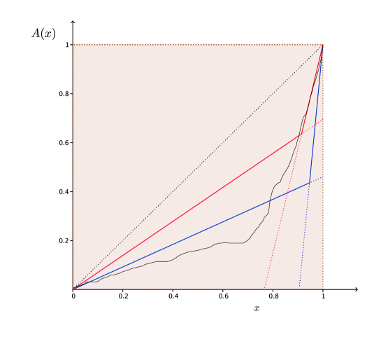
Figure 1. Gaussian Comparison: The extremal process of BBM with covariance $A$ (black curve) is compared to process with covariances functions $\overline{A}$ (red curve), respectively $\underline{A}$ (blue, curve).

Acknowledgements. We thank an anonymous referee for a very careful reading of our paper and for numerous valuable suggestions.

2. Localization of paths

In this section we show where the paths of particles that are extreme at time $t$ are localised. This is essentially inherited from properties of the standard Brownian bridge. For a given speed function $\Sigma^{2}$, and a subinterval $I\subset[0,t]$, define the following events on the space of paths, $X:{\mathbb{R}}_{+}\to{\mathbb{R}}$,

$${\mathcal{T}}_{t,I,\Sigma^{2}}^{\gamma}=\left\{X\Big{|}\forall s:s\in I:\left|X(s)-{\textstyle{\Sigma^{2}(s)\over t}}X(t)\right|<(\Sigma^{2}(s)\wedge(t-\Sigma^{2}(s)))^{\gamma}\right\}.$$ (2.1)

Proposition 2.1.

Let $x$ denote variable speed BBM with covariance function $A$. For $0\leq r<t$, set $I_{r}\equiv\{s:\Sigma^{2}(s)\in[r,t-r]\}$. For any ${\gamma}>\frac{1}{2}$ and for all $d\in{\mathbb{R}}$, for all $\epsilon>0$, there exists $r_{0}<\infty$ such that, for $r>r_{0}$ and for all $t>3r$,

$${\mathbb{P}}\left(\exists k\leq n(t):\left\{x_{k}(t)>\tilde{m}(t)+d\right\}\wedge\left\{x_{k}\not\in{\mathcal{T}}_{t,I_{r},\Sigma^{2}}^{\gamma}\right\}\right)<\epsilon.$$ (2.2)

To prove Proposition 2.1 we need the following lemma on Brownian bridges (see [13]).

Lemma 2.2.

Let ${\gamma}>\frac{1}{2}$. Let $\xi$ be a Brownian bridge from $0$ to $0$ in time $t$. Then, for all $\epsilon>0$, there exists $r_{0}<\infty$ such that, for $r>r_{0}$ and for all $t>3r$,

$${\mathbb{P}}\left(\exists s\in[r,t-r]:|\xi(s)|>(s\wedge(t-s))^{\gamma}\right)<\epsilon.$$ (2.3)

More precisely,

$${\mathbb{P}}\left(\exists s\in[r,t-r]:|\xi(s)|>(s\wedge(t-s))^{\gamma}\right)<8\sum_{k=\lfloor r\rfloor}^{\infty}k^{\frac{1}{2}-{\gamma}}\hbox{\rm e}^{-k^{2{\gamma}-1}/2}.$$ (2.4)

Proof.

The probability in (2.3) is bounded from above by

$$\sum_{k=\lceil r\rceil}^{\lceil t-r\rceil}{\mathbb{P}}\left(\exists s\in[k-1,k]:|\xi(s)|>(s\wedge(t-s))^{\gamma}\right)$$

$$\leq 2\sum_{k=\lceil r\rceil}^{\lceil t/2\rceil}{\mathbb{P}}\left(\exists s\in[k-1,k]:|\xi(s)|>(s\wedge(t-s))^{\gamma}\right),$$ (2.5)

by the reflection principle for the Brownian bridge. This is bounded from above by

$$2\sum_{k=\lceil r\rceil}^{\lceil t/2\rceil}{\mathbb{P}}\left(\exists s\in[0,k]:|\xi(s)|>(k-1)^{\gamma}\right).$$ (2.6)

Using the bound of Lemma 2.2 (b) of [13] we have

$$P\left(\exists s\in[0,k]:|\xi(s)|>(k-1)^{\gamma}\right)\leq 4(k-1)^{\frac{1}{2}-{\gamma}}\hbox{\rm e}^{-(k-1)^{2{\gamma}-1}/2}.$$ (2.7)

Using this bound for each summand in (2.6) we obtain (2.4). Since the sum on the right-hand side of (2.4) is finite (2.3) follows. ∎

Proof of Proposition 2.1.

Using a first moment method, the probability in (2.2) is bounded from above by

$$\hbox{\rm e}^{t}{\mathbb{P}}\left(B_{\Sigma^{2}(t)}>\tilde{m}(t)+d,B_{\Sigma^{2}(\cdot)}\not\in{\mathcal{T}}_{t,I_{r},\Sigma^{2}}^{\gamma}\right).$$ (2.8)

Since $\Sigma^{2}(s)$ is an non-decreasing function on $[0,t]$ with $\Sigma^{2}(t)=t$, the expression in (2.8) is bounded from above by

$$\hbox{\rm e}^{t}{\mathbb{P}}\left(\left\{B_{t}>\tilde{m}(t)+d\right\}\land\left\{\exists s\in[r,t-r]:\left|B_{s}-\frac{s}{t}B_{t}\right|>(s\wedge(t-s))^{\gamma}\right\}\right).$$ (2.9)

Now, $\xi(s)\equiv B_{s}-\frac{s}{t}B_{t}$ is the Brownian bridge from $0$ to $0$ in time $t$, and it is well known (see e.g. Lemma 2.1 in [13]) that $\xi(s)$ is independent of $B_{t}$, for all $s\in[0,t]$. Therefore, (2.9) is equal to

$$\hbox{\rm e}^{t}{\mathbb{P}}\left(B_{t}>\tilde{m}(t)+d\right){\mathbb{P}}\left(\exists s\in[r,t-r]:\left|\xi(s)\right|>(s\wedge(t-s))^{\gamma}\right).$$ (2.10)

Using the standard Gaussian tail bound,

$$\int_{u}^{\infty}\hbox{\rm e}^{-x^{2}/2}dx\leq u^{-1}\hbox{\rm e}^{-u^{2}/2},\quad\text{for}\,\,u>0,$$ (2.11)

we have

$$\hbox{\rm e}^{t}{\mathbb{P}}\left(B_{t}>\tilde{m}(t)+d\right) \leq \hbox{\rm e}^{t}\frac{\sqrt{t}}{\sqrt{2\pi}(\tilde{m}(t)+d)}\hbox{\rm e}^{-(\tilde{m}(t)+d)^{2}/2t}$$ (2.12)

$$\leq \frac{t}{\sqrt{2\pi}(\tilde{m}(t)+d)}\hbox{\rm e}^{-\sqrt{2}d}\leq M,$$

for some constant $M$ (depending on $d$), if $t$ is large enough. By Lemma 2.2 we can find $r_{0}$ large enough such that for all $r\geq r_{0}$ and $t>3r$,

$${\mathbb{P}}\left(\exists s\in[r,t-r]:\left|\xi(s)\right|>(s\wedge(t-s))^{\gamma}\right)<\epsilon/M.$$ (2.13)

The bounds (2.12) and (2.13) imply that (2.10) is smaller than $\epsilon$. ∎

3. Proof of Theorem 1.1

In this section we prove Theorem 1.1 assuming Proposition 3.2 below, whose proof will be postponed to the following two sections.

Proof of Theorem 1.1.

We show the convergence of the extremal process

$${\mathcal{E}}_{t}=\sum_{k\leq n(t)}{\delta}_{x_{k}(t)-\tilde{m}(t)}$$ (3.1)

by showing the convergence of the finite dimensional distributions and tightness. Tightness of $({\mathcal{E}}_{t})_{t\geq 0}$ is implied by the following bound on the number of particles above a level $d$ (see [37], Lemma 3.20).

Proposition 3.1.

For any $d\in{\mathbb{R}}$ and $\epsilon>0$, there exists $N=N(\epsilon,d)$ such that, for all $t$ large enough,

$${\mathbb{P}}\left({\mathcal{E}}_{t}[d,\infty)\geq N\right)<\epsilon.$$ (3.2)

Proof.

By a first order Chebyshev inequality, for all $t$ large enough,

$${\mathbb{P}}\left({\mathcal{E}}_{t}[d,\infty)\geq N\right)\leq\frac{1}{N}\hbox{\rm e}^{t}{\mathbb{P}}\left(B_{t}>\tilde{m}(t)+d\right)\leq\frac{M}{N}$$ (3.3)

by (2.12), where $M>0$ is a constant that depends on $d$. Choosing $N>M/\epsilon$ yields Proposition 3.1. ∎

To show the convergence of the finite dimensional distributions define, for $u\in{\mathbb{R}}$,

$${\mathcal{N}}_{u}(t)=\sum_{i=1}^{n(t)}\mathbbm{1}_{x_{i}(t)-\tilde{m}(t)>u},$$ (3.4)

that counts the number of points that lie above $u$. Moreover, we define the corresponding quantity for the process ${\mathcal{E}}_{{\sigma}_{b},{\sigma}_{e}}$ (defined in (1.13)),

$${\mathcal{N}}_{u}=\sum_{i,j}\mathbbm{1}_{p_{i}+{\sigma}_{e}{\Lambda}_{j}^{(i)}>u}.$$ (3.5)

Observe that, in particular,

$${\mathbb{P}}\left(\max_{1\leq i\leq n(t)}x_{i}(t)-\tilde{m}(t)\leq u\right)={\mathbb{P}}\left({\mathcal{N}}_{u}(t)=0\right).$$ (3.6)

The key step in the proof of Theorem 1.1 is the following proposition, that asserts the convergence of the finite dimensional distributions of the process ${\mathcal{E}}_{t}$.

Proposition 3.2.

For all $k\in{\mathbb{N}}$ and $u_{1},\dots,u_{k}\in{\mathbb{R}}$

$$\{{\mathcal{N}}_{u_{1}}(t),\dots,{\mathcal{N}}_{u_{k}}(t)\}\stackrel{{\scriptstyle d}}{{\to}}\{{\mathcal{N}}_{u_{1}},\dots,{\mathcal{N}}_{u_{k}}\}$$ (3.7)

as $t\uparrow\infty$.

The proof of this proposition will be postponed to the following sections.

Assuming the proposition, we can now conclude the proof of the theorem. The distribution of $\{{\mathcal{N}}_{u_{1}}(t),\dots,{\mathcal{N}}_{u_{k}}(t)\}$ for all $k\in{\mathbb{N}},u_{1},\dots,u_{k}\in{\mathbb{R}}$ characterise the finite dimensional distributions of the point process ${\mathcal{E}}_{t}$ since the class of sets $\{(u,\infty),u\in{\mathbb{R}}\}$ form a $\Pi$-system that generates ${\mathcal{B}}({\mathbb{R}})$. Hence (3.7) implies the convergence of the finite dimensional distributions of ${\mathcal{E}}_{t}$ (see, e.g., Proposition 3.4 in [37]).

Combining this observation with Propositions 3.1, we obtain Assertion (ii) of Theorem 1.1. Assertion (i) follows immediately from Eq. (3.6).

To prove Assertion (iii), we need to show that, as ${\sigma}^{2}_{e}\uparrow\infty$, it holds that $\widetilde{C}({\sigma}_{e})\uparrow 1/\sqrt{4\pi}$ and the processes ${\Lambda}^{(i)}$ converge to the trivial process ${\delta}_{0}$. Then,

$${\mathcal{E}}_{{\sigma}_{b},\infty}=\sum_{i}{\delta}_{p_{i}},$$ (3.8)

where $(p_{i},i\in{\mathbb{N}})$ are the points of a Cox process directed by the random measure

$\frac{1}{\sqrt{4\pi}}Y_{{\sigma}_{b}}\hbox{\rm e}^{-\sqrt{2}x}dx$.

Lemma 3.3.

The point process ${\mathcal{E}}_{{\sigma}_{b},{\sigma}_{e}}$ converges in law, as ${\sigma}_{e}\uparrow\infty$, to the point process ${\mathcal{E}}_{{\sigma}_{b},\infty}$.

Proof.

The proof of Lemma 3.3 is based on a result concerning the cluster processes ${\Lambda}^{(i)}$. We write ${\Lambda}_{{\sigma}_{e}}$ for a single copy of these processes and add the subscript to make the dependence on the parameter ${\sigma}_{e}$ explicit. We recall from [9] that the process ${\Lambda}_{{\sigma}_{e}}$ is constructed as follows. Define the processes $\overline{{\mathcal{E}}}_{{\sigma}_{e}}$ as the limits of the point processes

$$\overline{{\mathcal{E}}}_{{\sigma}_{e}}^{t}\equiv\sum_{k=1}^{n(t)}{\delta}_{x_{k}(t)-\sqrt{2}{\sigma}_{e}t}$$ (3.9)

where $x$ is standard BBM at time $t$ conditioned on the event $\{\max_{k\leq n(t)}x_{k}(t)>\sqrt{2}{\sigma}_{e}t\}$. We show here that, as ${\sigma}_{e}$ tends to infinity, the processes $\overline{{\mathcal{E}}}_{{\sigma}_{e}}$ converge to a point process consisting of a single atom at $0$. More precisely, we show that

$$\lim_{{\sigma}_{e}\uparrow\infty}\lim_{t\uparrow\infty}{\mathbb{P}}\left(\overline{\mathcal{E}}^{t}_{{\sigma}_{e}}([-R,\infty))>1\big{|}\max_{k\leq n(t)}x_{k}(t)>\sqrt{2}{\sigma}_{e}t\right)=0.$$ (3.10)

Now,

$${\mathbb{P}}\left(\overline{\mathcal{E}}^{t}_{{\sigma}_{e}}([-R,\infty))>1\big{|}\max_{k\leq n(t)}x_{k}(t)>\sqrt{2}{\sigma}_{e}t\right)$$ (3.11)

$$\leq{\mathbb{P}}\left(\mathop{\rm supp}\nolimits\overline{\mathcal{E}}^{t}_{{\sigma}_{e}}\cap[0,\infty)\neq\emptyset\land\overline{\mathcal{E}}^{t}_{{\sigma}_{e}}([-R,\infty))>1\big{|}\max_{k\leq n(t)}x_{k}(t)>\sqrt{2}{\sigma}_{e}t\right)$$

$$\leq\int_{0}^{\infty}{\mathbb{P}}\left(\mathop{\rm supp}\nolimits\overline{\mathcal{E}}^{t}_{{\sigma}_{e}}\cap dy\neq\emptyset\land\overline{\mathcal{E}}^{t}_{{\sigma}_{e}}([-R,\infty))>1\big{|}\max_{k\leq n(t)}x_{k}(t)>\sqrt{2}{\sigma}_{e}t\right)$$

$$=\int_{0}^{\infty}{\mathbb{P}}\left(\mathop{\rm supp}\nolimits\overline{\mathcal{E}}^{t}_{{\sigma}_{e}}\cap dy\neq\emptyset\big{|}\max_{k\leq n(t)}x_{k}(t)>\sqrt{2}{\sigma}_{e}t\right)$$

$$\qquad\times{\mathbb{P}}\left(\overline{\mathcal{E}}^{t}_{{\sigma}_{e}}([-R,\infty))>1\big{|}\mathop{\rm supp}\nolimits\overline{\mathcal{E}}^{t}_{{\sigma}_{e}}\cap dy\neq\emptyset\right).$$

But ${\mathbb{P}}\left(\cdot\big{|}\mathop{\rm supp}\nolimits\overline{\mathcal{E}}^{t}_{{\sigma}_{e}}\cap dy\neq\emptyset\right)\equiv P_{t,y+\sqrt{2}{\sigma}_{e}}(\cdot)$ is the Palm measure on BBM, i.e. the conditional law of BBM given that there is a particle at time $t$ in $dy$ (see Kallenberg [29, Theorem 12.8]. Chauvin, Rouault, and Wakolbinger [18, Theorem 2] describe the tree under the Palm measure $P_{t,z}$ as follows. Pick one particle at time $t$ at the location $z$. Then pick a spine, $Y$, which is a Brownian bridge from $0$ to $z$ in time $t$. Next pick a Poisson point process $\pi$ on $[0,t]$ with intensity $2$. For each point $p\in\pi$ start a random number $\nu_{p}$ of independent branching Brownian motions $({\mathcal{B}}^{Y(p),i},i\leq\nu_{p})$ starting at $Y(p)$. The law of $\nu$ is given by the size biased distribution, ${\mathbb{P}}(\nu_{p}=k-1)\sim\frac{kp_{k}}{2}$. See Figure LABEL:figure.1. Now let $z=\sqrt{2}{\sigma}_{e}t+y$ for $y\geq 0$. Under the Palm measure, the point process $\overline{{\mathcal{E}}}_{{\sigma}_{e}}(t)$ then takes the form

$$\overline{{\mathcal{E}}}_{{\sigma}_{e}}(t)\overset{\mathrm{law}}{=}{\delta}_{y}+\sum_{p\in\pi,i<\nu_{p}}\sum_{j=1}^{n_{Y(p),i}(p)}{\delta}_{{\mathcal{B}}^{Y(p),i}_{j}(t-p)-\sqrt{2}{\sigma}_{e}t}.$$ (3.12)

Since, for $1>{\gamma}>1/2$,

$$\lim_{{\sigma}_{e}\uparrow\infty}\lim_{t\uparrow\infty}{\mathbb{P}}\left(\forall s\geq{\sigma}_{e}^{-1/2}:Y(t-s)-y+\sqrt{2}{\sigma}_{e}s\in[-({\sigma}_{e}s)^{\gamma},({\sigma}_{e}s)^{\gamma}]\right)=1,$$ (3.13)

if we define the set

$${\mathcal{G}}^{t}_{{\sigma}_{e}}\equiv\left\{Y:\forall{t\geq s\geq{\sigma}_{e}^{-1/2}}:Y(t-s)-y+\sqrt{2}{\sigma}_{e}s\in[-({\sigma}_{e}s)^{\gamma},({\sigma}_{e}s)^{\gamma}]\right\},$$ (3.14)

it will suffice to show that, for all $R\in{\mathbb{R}}_{+}$,

$$\lim_{{\sigma}_{e}\uparrow\infty}\lim_{t\uparrow\infty}{\mathbb{P}}\left(\exists{p\in\pi,i<\nu_{p},j}:{{\mathcal{B}}^{Y(p),i}_{j}(t-p)\geq y-R}\land Y\in{\mathcal{G}}^{t}_{{\sigma}_{e}}\right)=0.$$ (3.15)

The probability in (3.15) is bounded by

$${\mathbb{P}}\left(\exists{p\in\pi,i\leq\nu_{p},j}:{{\mathcal{B}}^{Y(p),i}_{j}(t-p)\geq y-R)}\land Y\in{\mathcal{G}}^{t}_{{\sigma}_{e}}\right)$$

$$\leq {\mathbb{E}}\left[\int_{0}^{t}\sum_{i=1}^{\nu_{p}}\mathbbm{1}_{{\mathcal{B}}^{Y(p),i}_{j}(t-p)>y-R}\mathbbm{1}_{Y\in{\mathcal{G}}_{{\sigma}_{e}}}\pi(dp)\right]$$

$$\leq {\mathbb{E}}\left[\int_{0}^{t}{\mathbb{E}}\left[\sum_{i=1}^{\nu_{p}}\mathbbm{1}_{\max_{j}{\mathcal{B}}^{Y(p),i}_{j}(t-p)\geq y-R}\mathbbm{1}_{Y\in{\mathcal{G}}^{t}_{{\sigma}_{e}}}\big{|}{\mathcal{F}}^{\pi}\right]\pi(dp)\right]$$

$$\leq \int_{0}^{t}2K{\mathbb{P}}\left(\max_{j}{\mathcal{B}}^{Y(t-s)}_{j}\geq y-R\land Y\in{\mathcal{G}}^{t}_{{\sigma}_{e}}\right)ds.$$

Here we used the independence of the offspring BBM and that the conditional probability given the ${\sigma}$-algebra ${\mathcal{F}}^{\pi}$ generated by the Poisson process $\pi$ appearing in the integral over $\pi$ depends only on $p$. For the integral over $s$ up to $1/{\sigma}_{\epsilon}^{1/2}$, we just bound the integrand by $2K$. For larger values, we use the localisation provided by the condition that $Y\in{\mathcal{G}}_{{\sigma}_{e}}$, to get that the right hand side of (3) is not larger than

$$2K\int_{0}^{{\sigma}_{e}^{-1/2}}ds+2K\int_{{\sigma}_{e}^{-1/2}}^{t}\hbox{\rm e}^{s}{\mathbb{P}}(B(s)>-R+\sqrt{2}{\sigma}_{e}s-({\sigma}_{e}s)^{\gamma})ds.$$ (3.17)

(3.17) is by (2.11) bounded from above by

$$2K{\sigma}_{e}^{-1/2}+2K\int_{{\sigma}_{e}^{-1/2}}^{\infty}\hbox{\rm e}^{(1-{\sigma}_{e}^{2})s+\sqrt{2}{\sigma}_{e}(R+({\sigma}_{e}s)^{{\gamma}})}ds.$$ (3.18)

From this it follows that (3.18) (which does no longer depend on $t$) converges to zero, as ${\sigma}_{e}\uparrow\infty$, for any $R\in{\mathbb{R}}$. Hence we see that

$${\mathbb{P}}\left(\overline{\mathcal{E}}^{t}_{{\sigma}_{e}}([-R,\infty))>1\big{|}\mathop{\rm supp}\nolimits\overline{\mathcal{E}}^{t}_{{\sigma}_{e}}\cap dy\neq\emptyset\right)\downarrow 0,$$ (3.19)

uniformly in $y\geq 0$, as $t$ and then ${\sigma}_{e}$ tend to infinity. Next,

$$\int_{0}^{\infty}{\mathbb{P}}\left(\mathop{\rm supp}\nolimits\overline{\mathcal{E}}^{t}_{{\sigma}_{e}}\cap dy\neq\emptyset\big{|}\max_{k\leq n(t)}x_{k}(t)>\sqrt{2}{\sigma}_{e}t\right)$$

$$\leq\int_{0}^{\infty}{\mathbb{P}}\left(\max_{k\leq n(t)}x_{k}(t)\geq\sqrt{2}{\sigma}_{e}t+y\big{|}\max_{k\leq n(t)}x_{k}(t)>\sqrt{2}{\sigma}_{e}t\right).$$

But by Proposition 7.5 in [9] the probability in the integrand converges to $\exp(-\sqrt{2}{\sigma}_{e}y)$, as $t\uparrow\infty$. It follows from the proof that this convergence is unifomr in $y$, and hence by dominated convergence, the right-hand side of (3) is finite. Therefore, (3.10) holds. As a consequence, ${\Lambda}_{{\sigma}_{e}}$ converges to ${\delta}_{0}$.

It remains to show that the intensity of the Poisson process converges as claimed. Theorems 1 and 2 of [16] relate the constant $\widetilde{C}({\sigma}_{e})$ defined by (1.15) to the intensity of the shifted BBM conditioned to exceed the level $\sqrt{2}{\sigma}_{e}t$ as follows:

$$\frac{1}{\sqrt{4\pi}\widetilde{C}({\sigma}_{e})} = \lim_{s\uparrow\infty}\frac{{\mathbb{E}}\left[\sum_{k}\mathbbm{1}_{\bar{x}_{k}(s)>\sqrt{2}{\sigma}_{e}s}\right]}{{\mathbb{P}}\left(\max_{k}\bar{x}_{k}(s)>\sqrt{2}{\sigma}_{e}s\right)}$$

$$= \lim_{s\uparrow\infty}{{\mathbb{E}}\left[\sum_{k}\mathbbm{1}_{\bar{x}_{k}(s)-\max_{i}\bar{x}_{i}(s)>\sqrt{2}{\sigma}_{e}s-\max_{i}\bar{x}_{i}(s)}\big{|}\max_{k}\bar{x}_{k}(s)>\sqrt{2}{\sigma}_{e}s\right]}$$

$$= {\Lambda}_{{\sigma}_{e}}((-E,0]),$$

where, by Theorem 7.5 in [9], $E$ is a exponentially distributed random variable with parameter $\sqrt{2}{\sigma}_{e}$, independent of ${\Lambda}_{{\sigma}_{e}}$. As we have just shown that ${\Lambda}_{{\sigma}_{e}}\rightarrow{\delta}_{0}$, it follows that the right-hand side tends to one, as ${\sigma}_{e}\uparrow\infty$, and hence $\widetilde{C}({\sigma}_{e})\uparrow 1/\sqrt{4\pi}$. Hence the intensity measure of the PPP appearing in ${\mathcal{E}}_{{\sigma}_{b},{\sigma}_{e}}$ converges to the desired intensity measure $\frac{1}{\sqrt{4\pi}}Y_{{\sigma}_{b}}\hbox{\rm e}^{-\sqrt{2}x}dx$.
∎

This proves Assertion (iii) of Theorem 1.1. ∎

4. Proof of Proposition 3.2

We prove Proposition 3.2 via convergence of Laplace transforms. For $u_{1},\dots,u_{k}\in{\mathbb{R}},k\in{\mathbb{N}}$, define the Laplace transform of $\{{\mathcal{N}}_{u_{1}}(t),\dots,{\mathcal{N}}_{u_{k}}(t)\}$,

$${\mathcal{L}}_{u_{1},\dots,u_{k}}(t,c)={\mathbb{E}}\left(\exp\left(-\sum_{l=1}^{k}c_{l}{\mathcal{N}}_{u_{l}}(t)\right)\right),\quad c=(c_{1},\dots,c_{k})^{t}\in{\mathbb{R}}_{+}^{k},$$ (4.1)

and analogously the Laplace transform ${\mathcal{L}}_{u_{1},\dots,u_{k}}(c)$ of $\{{\mathcal{N}}_{u_{1}},\dots,{\mathcal{N}}_{u_{k}}\}$. Proposition 3.2 is then a consequence of the next proposition.

Proposition 4.1.

For any $k\in{\mathbb{N}}$, $u_{1},\dots,u_{k}\in{\mathbb{R}}$ and $c_{1},\dots,c_{k}\in{\mathbb{R}}_{+}$

$$\lim_{t\to\infty}{\mathcal{L}}_{u_{1},\dots,u_{k}}(t,c)={\mathcal{L}}_{u_{1},\dots,u_{k}}(c).$$ (4.2)

The proof of Proposition 4.1 comes in two main steps. First, we prove the result for the case of two speed BBM. This was done in our previous paper [9]. In fact, we will need a slight extension of that result where we allow a slight dependence of the speeds on $t$. This will be given in the next subsection.

The second step is to show that, under the hypotheses of Theorem 1.1, the Laplace transforms can be well approximated by those of two speed BBM. This uses the classical Gaussian comparison argument in a slightly subtle way.

4.1. Approximating two speed BBM. The case $A^{\prime}(1)<\infty$.

It turns out that it is enough to compare the process with covariance function $A$ with processes whose covariance function is piecewise linear with a single change in slope. We derive asymptotic upper and lower bounds by choosing these in such a way that the covariances near zero and near one are below, respectively above, that of the original process. We define

$${\delta}^{<}(t) = \sup\{x\in[0,1]:A(x)\leq t^{-2/3}\}$$

$${\delta}^{>}(t) = 1-\inf\{x\in[0,1]:A(x)\geq 1-t^{-2/3}\}$$ (4.3)

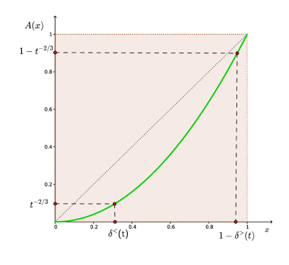
(a) Case 1) ${\sigma}_{b}=0$ but $\lim_{t\uparrow\infty}{\delta}^{<}(t)=0$

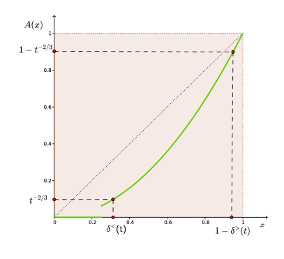
(b) Case 2) ${\sigma}_{b}=0$ but $\lim_{t\uparrow\infty}{\delta}^{<}(t)={\delta}^{<}\neq 0$

Figure 3. Different cases for ${\delta}^{<}(t)$ and ${\delta}^{>}(t)$.

By Assumption (A1) it follows that $\lim_{t\uparrow\infty}{\delta}^{>}(t)=0$.

Remark.

If $\lim_{t\uparrow\infty}{\delta}^{<}(t)={\delta}^{<}\neq 0$, then it follows from the definition of ${\delta}^{<}(t)$ that $A(x)=0$ on $[0,{\delta}^{<}]$.

In the following formulas, we choose a parameter $n\in{\mathbb{N}}_{\geq 2}$ as follows. If in Assumption (A2) the functions $\overline{B},\underline{B}$ can be chosen such that there exists $m\geq 2$, such that $\underline{B}^{(k)}(0)=\overline{B}^{(k)}(0)=0$, for all $1\leq k<m$, and in some finite interval $[0,{\delta}_{b}]$, both $|\underline{B}^{(m)}(x)|$ and $|\overline{B}^{(m)}(x)|$ are bounded by some constants $\underline{K}_{1}$, respectively $\overline{K}_{1}$, then we choose $n$ as the largest of these integers. Otherwise, we choose $n=2$. Moreover, let $|\overline{C}^{\prime\prime}(x)|\leq\overline{K}_{2}$ and $|\underline{C}^{\prime\prime}(x)|\leq\underline{K}_{2}$ for all $x\in[1-{\delta}_{e},1]$. We define

$$\overline{\Sigma}^{2}(s)=t\overline{A}(s/t)$$ (4.4)

and

$$\underline{\Sigma}^{2}(s)=t\underline{A}(s/t).$$ (4.5)

Here

$$\overline{A}(x)=\begin{cases}({\sigma}_{b}^{2}+\frac{\overline{K}_{1}}{n!}({\delta}^{<}(t))^{n-1})x,&0\leq x\leq\overline{b},\\ 1+({\sigma}_{e}^{2}-\frac{\overline{K}_{2}}{2}{\delta}^{>}(t))(x-1),&\overline{b}<x\leq 1,\end{cases}$$ (4.6)

with

$$\overline{b}=\frac{1-{\sigma}_{e}^{2}+\frac{\overline{K}_{2}}{2}{\delta}^{>}(t)}{{\sigma}_{b}^{2}+\frac{\overline{K}_{1}}{n!}({\delta}^{<}(t))^{n-1}-{\sigma}_{e}^{2}+\frac{\overline{K}_{2}}{2}{\delta}^{>}(t)}.$$ (4.7)

If ${\sigma}^{2}_{e}<\infty$,

$$\underline{A}(x)=\begin{cases}\left\{({\sigma}_{b}^{2}-\frac{\underline{K}_{1}}{n!}({\delta}^{<}(t))^{n-1})x\right\}\vee 0,&0\leq x\leq\underline{b},\\ 1+({\sigma}_{e}^{2}+\frac{\underline{K}_{2}}{2}{\delta}^{>}(t))(x-1),&\underline{b}<x\leq 1,\end{cases}$$ (4.8)

with

$$\underline{b}=\frac{1-{\sigma}_{e}^{2}-\frac{\underline{K}_{2}}{2}{\delta}^{>}(t)}{{\sigma}_{b}^{2}-\frac{\underline{K}_{1}}{n!}({\delta}^{<}(t))^{n-1}-{\sigma}_{e}^{2}-\frac{\underline{K}_{2}}{2}{\delta}^{>}(t)}.$$ (4.9)

Remark.

If ${\sigma}^{2}_{b}=0$, $\underline{A}(x)=0$ for $0\leq x\leq\underline{b}$. If $\lim_{t\uparrow\infty}{\delta}^{<}(t)={\delta}^{<}\neq 0$ (which implies that all derivatives in zero are $0$), we take

$$\overline{A}(x)=\begin{cases}0,&0\leq x\leq\overline{b},\\ 1+({\sigma}_{e}^{2}-\frac{\overline{K}_{2}}{2}{\delta}^{>}(t))(x-1),&\overline{b}<x\leq 1,\end{cases}$$ (4.10)

and

$$\overline{b}=\frac{1-{\sigma}_{e}^{2}+\frac{\overline{K}_{2}}{2}{\delta}^{>}(t)}{-{\sigma}_{e}^{2}+\frac{\overline{K}_{2}}{2}{\delta}^{>}(t)}.$$ (4.11)

If $A^{\prime}(1)={\sigma}^{2}_{e}=+\infty$, then $\underline{b}=1$. And $\overline{A}\equiv\overline{A}_{\rho}$ is defined by

$$\overline{A}(x)=\begin{cases}({\sigma}_{b}^{2}+\frac{\overline{K}_{1}}{n!}({\delta}^{<}(t))^{n-1})x,&0\leq x\leq\overline{b},\\ 1+\rho(x-1),&\overline{b}<x\leq 1,\end{cases}$$ (4.12)

and $\overline{b}\equiv\overline{b}_{\rho}=\frac{1-\rho}{{\sigma}_{b}^{2}+\frac{\overline{K}_{1}}{n!}({\delta}^{<}(t))^{n-1}-\rho}$.

The choice of $\overline{\Sigma}^{2}$ and $\underline{\Sigma}^{2}$ is motivated by the following properties.

Lemma 4.2.

$\overline{A}$ and $\underline{A}$ are piecewise linear, continuous functions with $\overline{A}(0)=\underline{A}(0)=0$ and $\overline{A}(1)=\underline{A}(1)=1$. Moreover,

• If $\lim_{t\uparrow\infty}{\delta}^{<}(t)=0$, then, for all $s$ with $\Sigma^{2}(s)\in[0,t^{1/3}]$ and $\Sigma^{2}(s)\in[t-t^{1/3},t]$,

  $$\overline{\Sigma}^{2}(s)\geq\Sigma^{2}(s)\geq\underline{\Sigma}^{2}(s).$$ (4.13)

• If $\lim_{t\uparrow\infty}{\delta}^{<}(t)={\delta}^{<}>0$, then (4.13) only holds for all $s$ with $\Sigma^{2}(s)\in[t-t^{1/3},t]$ while, for $s\in[0,({\delta}\land\overline{b})t)$,

  $$\overline{\Sigma}^{2}(s)=\Sigma^{2}(s)=\underline{\Sigma}^{2}(s)=0.$$ (4.14)

Proof.

$\overline{A}$ and $\underline{A}$ are obviously piecewise linear. The fact that they are continuous is easily verified. By definition, $A^{\prime}(0)={\sigma}_{b}^{2}$ and $A^{\prime}(1)={\sigma}_{e}^{2}$. For all $s$ such that $\Sigma^{2}(s)\in[0,t^{1/3}]$, a $n$th-order Taylor expansion of $\overline{B}$ at $0$ together with the fact that by assumption, for $k<n$, $\overline{B}(0)=\overline{B}^{k}(0)=0$ shows that

$$\Sigma^{2}(s)\leq\overline{B}(s)=t\left[\overline{B}^{\prime}(0)\frac{s}{t}+\frac{\overline{B}^{(n)}(\xi)}{n!}\left(\frac{s}{t}\right)^{n}\right],\quad\mbox{for some }\xi\in(0,s).$$ (4.15)

The reverse inequality holds when $\overline{B}$ is replaced by $\underline{B}$. Eq. (4.13) follows then from Assumption (A2). Using a second order Taylor expansion of $\overline{C}$ and $\underline{C}$ at $1$, we obtain Eq. (4.13) for $\Sigma^{2}(s)\in[t-t^{1/3},t]$. Eq. (4.14) holds trivially in the specified interval. This concludes the proof of the lemma. ∎

Let $\{\overline{y}_{i},i\leq n(t)\}$ be the particles of a BBM with speed function $\overline{\Sigma}^{2}$ and let
$\{\underline{y}_{i},i\leq n(t)\}$ be particles of a BBM with speed function $\underline{\Sigma}^{2}$. We want to show that the limiting extremal processes of these processes coincide. Set

$$\overline{{\mathcal{N}}}_{u}(t)\equiv\sum_{i=1}^{n(t)}\mathbbm{1}_{\overline{y}_{i}(t)-\tilde{m}(t)>u},$$ (4.16)

$$\underline{{\mathcal{N}}}_{u}(t)\equiv\sum_{i=1}^{n(t)}\mathbbm{1}_{\underline{y}_{i}(t)-\tilde{m}(t)>u}.$$ (4.17)

Lemma 4.3.

For all $u_{1},\dots,u_{k}$ and all $c_{1},\dots,c_{k}\in{\mathbb{R}}_{+}$, the limits

$$\lim_{t\uparrow\infty}{\mathbb{E}}\left(\exp\left(-\sum_{l=1}^{k}c_{k}\overline{{\mathcal{N}}}_{u_{l}}(t)\right)\right)$$ (4.18)

and

$$\lim_{t\uparrow\infty}{\mathbb{E}}\left(\exp\left(-\sum_{l=1}^{k}c_{k}\underline{{\mathcal{N}}}_{u_{l}}(t)\right)\right)$$ (4.19)

exist. If $A^{\prime}(1)<\infty$, then two limits coincide with ${\mathcal{L}}_{u_{1},\dots,u_{k}}(c)$.

If $A^{\prime}(1)={\sigma}_{e}^{2}=\infty$, then the two limits in (4.18) and (4.19) converges to the same limit, as $\rho\uparrow\infty$.

Proof.

We first consider the case when $A^{\prime}(1)<\infty$. To prove Lemma 4.3, we show that the extremal processes

$$\overline{{\mathcal{E}}_{t}}=\sum_{i=1}^{n(t)}{\delta}_{\overline{y}_{i}-\tilde{m}(t)}\quad\mbox{and}\quad\underline{{\mathcal{E}}_{t}}=\sum_{i=1}^{n(t)}{\delta}_{\underline{y}_{i}-\tilde{m}(t)}$$ (4.20)

both converge to ${\mathcal{E}}_{{\sigma}_{b},{\sigma}_{e}}$, that was defined in (1.13). Note that this implies first convergence of Laplace functionals with functions $\phi$ with compact support, while the ${\mathcal{N}}_{u}(t)$ have support that is unbounded from above. Convergence for these, however, carries over due to the tightness established in Proposition 3.1.

To do so, observe that the slopes at $0$ of $\overline{\Sigma}^{2}$ and $\underline{\Sigma}^{2}$ are equal to ${\sigma}_{b}^{2}$ up to an error of order ${\delta}^{<}(t)$. Moreover, the slope at $t$ is in both cases, up to an error of order ${\delta}^{>}(t)$, equal to ${\sigma}_{e}^{2}$. The time of speed change $\overline{b}(t)$, respectively $\underline{b}(t)$, is equal to $\frac{1-{\sigma}_{e}^{2}}{{\sigma}_{b}^{2}-{\sigma}_{b}^{2}}$ up to an error of order ${\delta}^{>}(t)\vee{\delta}^{<}(t)$. For the two-speed BBM with speed

$${\sigma}^{2}(s)=\begin{cases}{\sigma}^{2}_{b},&\,\hbox{for}\,\,0<s\leq\frac{1-{\sigma}_{e}^{2}}{{\sigma}_{b}^{2}-{\sigma}_{e}^{2}},\\ {\sigma}^{2}_{e},&\,\hbox{for}\,\,\frac{1-{\sigma}_{e}^{2}}{{\sigma}_{b}^{2}-{\sigma}_{e}^{2}}<s<t,\end{cases}$$ (4.21)

it was shown in [9] that the maximal displacement is equal to $\tilde{m}(t)$ and that the extremal process converges to ${\mathcal{E}}_{{\sigma}_{b},{\sigma}_{e}}$ as $t\uparrow\infty$. The method used to show this is to show the convergence of the Laplace functionals, ${\mathbb{E}}(\exp(-\int\phi(x){\mathcal{E}}_{t}(dx)))$, $\phi\in C_{c}({\mathbb{R}},{\mathbb{R}}_{+})$. The other difference is that the function $A$ we have to consider now depend (weakly) on $t$. We need to show that this has no effect.

Inspecting the proof of the convergence of the Laplace functional, respectively convergence of the maximum in [9], one sees that nothing changes (since we keep $t$ fixed) until Eq. (5.28) in [9]. There, we then have to show that, for each $y\in{\mathbb{R}}$, (in the case of $\overline{\Sigma}^{2}$)

$${\mathbb{E}}\left(\exp\left(-C(a)\left({\textstyle{{\sigma}_{e}^{2}-\frac{\overline{K}_{2}}{2}{\delta}^{>}(t)\over 1-[{\sigma}_{b}^{2}+\frac{\overline{K}_{1}}{2}{\delta}^{<}(t)]\overline{b}/\sqrt{t}}}\right)^{1/2}\hbox{\rm e}^{-\sqrt{2}y}\overline{Y}_{{\sigma}_{b},\overline{b}\sqrt{t},{\gamma}}^{B}\right)(1+o(1))\right),$$ (4.22)

converges, as first $t\uparrow\infty$ and then $B\uparrow\infty$, to

$${\mathbb{E}}\left(\exp\left(-{\sigma}_{e}C(a)Y_{{\sigma}_{b}}\hbox{\rm e}^{-\sqrt{2}y}\right)\right),$$ (4.23)

where $C(a)>0$ is a constant depending on $a=\sqrt{2}({\sigma}_{e}-1)$ (see (1.15)), and

$$\overline{Y}_{{\sigma}_{b},\overline{b}\sqrt{t},{\gamma}}^{B}=\sum_{i=1}^{n(\overline{b}\sqrt{t})}\hbox{\rm e}^{-(1+{\sigma}_{b}^{2}+\frac{K}{2}{\delta}^{<}(t))\overline{b}\sqrt{t}+\sqrt{2}\overline{y}_{i}(\overline{b}\sqrt{t})}\mathbbm{1}_{\overline{y}_{i}(\overline{b}\sqrt{t})-\sqrt{2}({\sigma}_{b}^{2}+\frac{K}{2}{\delta}^{<}(t))\overline{b}\sqrt{t}\in[-Bt^{{\gamma}/2},Bt^{{\gamma}/2}]}.$$ (4.24)

The main task is to ensure the convergence of $\overline{Y}_{{\sigma}_{b},\overline{b}\sqrt{t},{\gamma}}^{B}$ to the limit of the corresponding McKean martingale, $Y_{{\sigma}_{b}}$. In the case where $\lim_{t\uparrow\infty}{\delta}^{<}(t)>0$, this takes the simple form

$$\overline{Y}_{0,\overline{b}\sqrt{t},{\gamma}}^{B}=\sum_{i=1}^{n(\overline{b}\sqrt{t})}\hbox{\rm e}^{-\overline{b}\sqrt{t}},$$ (4.25)

which converges to an exponential random variable of mean one, as desired.

In the case when $\lim_{t\uparrow\infty}{\delta}^{<}(t)=0$, a further slight modification is necessary. Observe that in the proof of Theorem 5.1 in [9], $\overline{b}\sqrt{t}$ can be replaced by any sequence ${\Delta}(t)\uparrow\infty$ such that $\lim_{t\uparrow\infty}{\Delta}(t)/t=0$. Here we adapt ${\Delta}(t)$ to the function $\Sigma^{2}$ and choose

$${\Delta}(t)=\left({\delta}^{<}(t)\right)^{-1/2}.$$ (4.26)

Doing so, we have to show that, analogously to (4.22), the object

$${\mathbb{E}}\left(\exp\left(-C(a)\left({\textstyle{{\sigma}_{e}^{2}-\frac{\overline{K}_{2}}{2}{\delta}^{>}(t)\over 1-[{\sigma}_{b}^{2}+\frac{\overline{K}_{1}}{2}{\delta}^{<}(t)]{\Delta}(t)/t}}\right)^{1/2}\hbox{\rm e}^{-\sqrt{2}y}\overline{Y}_{{\sigma}_{b},{\Delta}(t),{\gamma}}^{B}\right)(1+o(1))\right)$$ (4.27)

converges to (4.23). By our choice of ${\Delta}(t)$,

$$\left|\hbox{\rm e}^{-\frac{\overline{K}_{1}}{2}{\delta}^{<}(t){\Delta}(t)}\hbox{\rm e}^{\sqrt{2}\frac{\overline{K}_{1}}{2}{\delta}^{<}(t)({\Delta}(t)+B{\Delta}(t)^{\gamma})}-1\right|\leq const.\sqrt{{\delta}^{<}(t)},$$ (4.28)

which tends to zero, as $t\uparrow\infty$. Thus

$$\overline{Y}_{{\sigma}_{b},{\Delta}(t),{\gamma}}^{B}=\widetilde{Y}_{{\sigma}_{b},{\Delta}(t),{\gamma}}^{B}(1+o(1)),$$ (4.29)

where

$$\widetilde{Y}_{{\sigma}_{b},{\Delta}(t),{\gamma}}^{B}\equiv\sum_{i=1}^{n({\Delta}(t))}\hbox{\rm e}^{-(1+{\sigma}_{b}^{2}){\Delta}(t)+\sqrt{2}{\sigma}_{b}\overline{x}_{i}({\Delta}(t))}\mathbbm{1}_{{\sigma}_{b}\overline{x}_{i}({\Delta}(t))-\sqrt{2}{\sigma}_{b}^{2}{\Delta}(t)\in[-B{\Delta}(t)^{{\gamma}},B{\Delta}(t)^{{\gamma}}]}.$$ (4.30)

By Lemma 4.3 in [9], it follows that $\widetilde{Y}_{{\sigma}_{b},{\Delta}(t),{\gamma}}^{B}$ converges in probability and in $L^{1}$ to the random variable $Y_{{\sigma}_{b}}$. Since $\widetilde{Y}_{{\sigma}_{b},{\Delta}(t),{\gamma}}^{B}\geq 0$ and $C(a)>0$, and since

$$\lim_{t\uparrow\infty}\left({\textstyle{{\sigma}_{e}^{2}-\frac{\overline{K}_{2}}{2}{\delta}^{>}(t)\over 1-[{\sigma}_{b}^{2}+\frac{\overline{K}_{1}}{2}{\delta}^{<}(t)]{\Delta}(t)/t}}\right)^{1/2}={\sigma}_{e},$$ (4.31)

it follows that

$$\lim_{B\uparrow\infty}\liminf_{t\uparrow\infty}{\mathbb{E}}\left(\exp\left(-C(a){\sigma}_{e}\hbox{\rm e}^{-\sqrt{2}y}\widetilde{Y}_{{\sigma}_{b},{\Delta}(t),{\gamma}}^{B}\right)(1+o(1))\right)$$

$$=\lim_{B\uparrow\infty}\limsup_{t\uparrow\infty}{\mathbb{E}}\left(\exp\left(-C(a){\sigma}_{e}\hbox{\rm e}^{-\sqrt{2}y}\widetilde{Y}_{{\sigma}_{b},{\Delta}(t),{\gamma}}^{B}\right)(1+o(1))\right)$$

$$={\mathbb{E}}\left(\exp\left(-\widetilde{C}({\sigma}_{e})Y_{{\sigma}_{b}}\hbox{\rm e}^{-\sqrt{2}y}\right)\right),$$ (4.32)

where $\widetilde{C}({\sigma}_{e})={\sigma}_{e}C(a)$. The same arguments work when $\overline{\Sigma}^{2}$ is replaced by $\underline{\Sigma}^{2}$. The limit in (4.1) coincides with the one obtained in [9] for the two-speed BBM with speed given in (4.21). The assertion in the case when ${\sigma}_{e}=\infty$ follows directly from Lemma 3.3. ∎

4.2. Gaussian comparison

We distinguish from now on the expectation with respect to the underlying tree structure and the one with respect to the Brownian movement of the particles.

• ${\mathbb{E}}_{n}$: expectation w.r.t. Galton-Watson process.

• ${\mathbb{E}}_{B}$: expectation w.r.t. the Gaussian process conditioned on the ${\sigma}$-algebra ${\mathcal{F}}_{t}^{\hbox{\tiny tree}}$ generated by the Galton Watson process.

For a given realisation of the Galton-Watson process, we now let $x$, $\bar{y}$, and $\underline{y}$ be three independent Gaussian processes whose covariances are given as in (1.2) with $A$ replaced by $\overline{A}$ in the case of $\bar{y}$ and $\underline{A}$ in the case of $\underline{y}$.

The proof of Proposition 4.1 is based on the following Lemma that compares the Laplace transform ${\mathcal{L}}_{u_{1},\dots,u_{k}}(t,c)$ with the corresponding Laplace transform for the comparison processes.

Lemma 4.4.

For any $k\in{\mathbb{N}}$, $u_{1},\dots,u_{k}\in{\mathbb{R}}$ and $c_{1},\dots,c_{k}\in{\mathbb{R}}_{+}$ we have

$${\mathcal{L}}_{u_{1},\dots,u_{k}}(t,c) \leq {\mathbb{E}}\left(\exp\left(-\sum_{l=1}^{k}c_{l}\overline{{\mathcal{N}}}_{u_{l}}(t)\right)\right)+o(1)$$ (4.33)

$${\mathcal{L}}_{u_{1},\dots,u_{k}}(t,c) \geq {\mathbb{E}}\left(\exp\left(-\sum_{l=1}^{k}c_{l}\underline{{\mathcal{N}}}_{u_{l}}(t)\right)\right)+o(1)$$ (4.34)

Proof.

The proofs of (4.33) and (4.34) are very similar. Hence we focus on proving (4.33). We will, however, indicate what has to be changed when proving the lower bound as we go along. For simplicity all overlined names depend on $\overline{\Sigma}^{2}$. Corresponding quantities where $\overline{\Sigma}^{2}$ is replaced by $\underline{\Sigma}^{2}$ are underlined.

To use Gaussian comparison methods, we first replace the functions ${\mathcal{N}}_{u}(t),\overline{\mathcal{N}}_{u}(t)$ by smooth approximants:

$$\chi^{\kappa}(x)\equiv\frac{1}{\sqrt{2\pi{\kappa}^{2}}}\int_{-\infty}^{x}\hbox{\rm e}^{-z^{2}/2{\kappa}^{2}}dz,$$ (4.35)

$${\mathcal{N}}^{\kappa}_{u}(t)\equiv\sum_{i=1}^{n(t)}\chi^{\kappa}(x_{i}(t)-\tilde{m}(t)-u),$$ (4.36)

and

$$\overline{{\mathcal{N}}}^{\kappa}_{u}(t)\equiv\sum_{i=1}^{n(t)}\chi^{\kappa}(\bar{y}_{i}(t)-\tilde{m}(t)-u).$$ (4.37)

Note that, as ${\kappa}\downarrow 0$,

$$\chi^{\kappa}(x)\rightarrow\mathbbm{1}_{x>0},\quad{\mathcal{N}}_{u}^{\kappa}(t)\rightarrow{\mathcal{N}}_{u}(t),\quad\overline{{\mathcal{N}}}_{u}^{\kappa}(t)\rightarrow\overline{{\mathcal{N}}}_{u}(t).$$ (4.38)

In order to prove (4.33), we show that for all ${\kappa}>0$,

$${\mathbb{E}}_{B}\left(\exp\left(-\sum_{l=1}^{k}c_{l}{{\mathcal{N}}}^{\kappa}_{u_{l}}(t)\right)\right)\leq{\mathbb{E}}_{B}\left(\exp\left(-\sum_{l=1}^{k}c_{l}\overline{{\mathcal{N}}}^{\kappa}_{u_{l}}(t)\right)\right)+R(t),$$ (4.39)

where $R(t)$ is independent of ${\kappa}$ and $\lim_{t\uparrow\infty}{\mathbb{E}}R(t)=0$.

From now on we work conditional on the ${\sigma}$-algebra generated by the Galton-Watson tree. We introduce the family of functions $f_{t,{\kappa}}:{\mathbb{R}}^{n(t)}\rightarrow{\mathbb{R}}$ by

$$f_{t,{\kappa}}(x)\equiv f_{t,{\kappa}}(x_{1},\dots,x_{n(t)})\equiv\exp\left(-\sum_{i=1}^{n(t)}\sum_{l=1}^{k}c_{l}\chi^{\kappa}(x_{i}-\tilde{m}(t)-u_{l})\right).$$ (4.40)

We want to control

$${\mathbb{E}}_{B}\left(\exp\left(-\sum_{l=1}^{k}c_{l}{\mathcal{N}}^{\kappa}_{u_{l}}(t)\right)\right)-{\mathbb{E}}_{B}\left(\exp\left(-\sum_{l=1}^{k}c_{l}\overline{{\mathcal{N}}}^{\kappa}_{u_{l}}(t)\right)\right)$$

$$={\mathbb{E}}_{B}\left(f_{t,{\kappa}}(x_{1}(t),\dots,x_{n(t)}(t))\right)-{\mathbb{E}}_{B}\left(f_{t,{\kappa}}(\overline{y}_{1}(t),\dots,\overline{y}_{n(t)}(t)))\right.$$ (4.41)

Define for $h\in[0,1]$ the interpolating process

$$x_{i}^{h}=\sqrt{h}x_{i}+\sqrt{1-h}\overline{y}_{i},\quad h\in[0,1].$$ (4.42)

The interpolating process $\{x_{i}^{h},i\leq n(t)\}$ is a Gaussian process with the same underlying branching structure and speed function

$$\Sigma_{h}^{2}(s)=h\Sigma^{2}(s)+(1-h)\overline{\Sigma}^{2}(s).$$ (4.43)

Then, (4.2) is equal to

$${\mathbb{E}}_{B}\left(\int_{0}^{1}\frac{d}{dh}f_{t,{\kappa}}(x^{h}(t))dh\right),$$ (4.44)

where

$$\frac{d}{dh}f_{t,{\kappa}}(x^{h}(t))=\frac{1}{2}\sum_{i=1}^{n(t)}\frac{\partial}{\partial x_{i}}f_{t,{\kappa}}(x_{1}^{h}(t),\dots,x_{n(t)}^{h}(t))\left[\frac{1}{\sqrt{h}}x_{i}(t)-\frac{1}{\sqrt{1-h}}\overline{y}_{i}(t)\right],$$ (4.45)

and derivative:

$$\frac{\partial}{\partial x_{i}}f_{t,{\kappa}}(x_{1}^{h}(t),\dots,x_{n(t)}^{h}(t))=-\left(\sum_{l=1}^{k}\frac{c_{l}}{\sqrt{2\pi{\kappa}^{2}}}\hbox{\rm e}^{-\frac{(x_{i}^{h}(t)-\tilde{m}(t)-u_{l})^{2}}{2{\kappa}^{2}}}\right)f_{t,{\kappa}}(x_{1}^{h}(t),\dots,x_{n(t)}^{h}(t)).$$ (4.46)

The key idea is to introduce a localisation condition on the path of $x_{i}^{h}$ into (4.45) at this stage. Note that it is not surprising at this point, since localising paths has been a crucial tool in almost all computations involving BBM, see already Bramson’s paper [14]. To do so, we insert into the right-hand side of (4.45) a one in the form

$$1=\mathbbm{1}_{x_{i}^{h}\in{\mathcal{T}}_{t,\bar{I},\Sigma_{h}^{2}}^{\gamma}}+\mathbbm{1}_{x_{i}^{h}\not\in{\mathcal{T}}_{t,\bar{I},\Sigma_{h}^{2}}^{\gamma}},$$ (4.47)

with

$$\bar{I}\equiv\left[t({\delta}^{<}_{0}(t)\land{\delta}^{<}_{1}(t)),t(1-{\delta}^{>}_{1}(t))\right],$$ (4.48)

and ${\mathcal{T}}_{t,I,\Sigma_{h}^{2}}^{\gamma}$ defined in (2.1). Here ${\delta}_{1}^{<,>}(t)\equiv{\delta}^{<,>}(t)$, while ${\delta}_{0}^{<,>}$ is defined in the same way, but with respect to the speed function $\overline{\Sigma}^{2}$ instead of $\Sigma^{2}$. We call the two resulting summands $\overline{S}^{h}_{<}$ and $\overline{S}^{h}_{>}$, respectively.

Note that, when proving the lower bound, we choose instead of $\bar{I}$, the interval

$$\underline{I}\equiv\left[t({\delta}^{<}_{0}(t)\land{\delta}^{<}_{1}(t)),t(1-{\delta}^{>}_{0}(t))\right].$$ (4.49)

The next lemma shows that $\overline{S}^{h}_{>}$ does not contribute to the expectation in (4.45), as $t\to\infty$.

Lemma 4.5.

With the notation above, we have

$$\lim_{t\to\infty}{\mathbb{E}}_{n}\left(\int_{0}^{1}{\mathbb{E}}_{B}(|\overline{S}^{h}_{>}|)dh\right)=0.$$ (4.50)

The proof of this lemma will be postponed.

We continue with the proof of Lemma 4.4. We are left with controlling, for fixed $h\in(0,1)$,

$${\mathbb{E}}_{B}(\overline{S}^{h}_{<})={\mathbb{E}}_{B}\left(\frac{1}{2}\sum_{i=1}^{n(t)}\frac{\partial}{\partial x_{i}}f_{t,{\kappa}}(x^{h}(t))\mathbbm{1}_{x_{i}^{h}\in{\mathcal{T}}_{t,\bar{I},\Sigma_{h}^{2}}^{\gamma}}\left[\frac{x_{i}(t)}{\sqrt{h}}-\frac{\overline{y}_{i}(t)}{\sqrt{1-h}}\right]\right).$$ (4.51)

By the definition of ${\mathcal{T}}_{t,\bar{I},\Sigma_{h}^{2}}^{\gamma}$,

$$\mathbbm{1}_{x_{i}^{h}\in{\mathcal{T}}_{t,\bar{I},\Sigma_{h}^{2}}^{\gamma}}=\mathbbm{1}_{\forall s\in\bar{I}:\left|\xi_{i}^{h}(s)\right|\leq(\Sigma_{h}^{2}(s)\wedge(t-\Sigma_{h}^{2}(s)))^{\gamma}},$$ (4.52)

where $\xi^{h}_{i}(s)\equiv x_{i}^{h}(s)-\frac{\Sigma_{h}^{2}(s)}{t}x^{h}_{i}(t)$ is a time changed Brownian bridge from $0$ to $0$ in time $t$, which, as we recall, is independent of the endpoint $x_{i}^{h}(t)$. We want to apply a Gaussian integration by parts formula to (4.51). However, we need to take care of the fact that each summand in (4.51) depends on the whole path of $\xi_{i}$ through the term in (4.52). Therefore, we first approximate that indicator function in (4.52) by a discretised version. Let, for $N\in{\mathbb{N}}$, $t_{1},\dots,t_{2^{N}}$ be a sequence of equidistant points in $[0,t]$. Define the following sequence of approximations, $G_{h,N}:C({\mathbb{R}}_{+})\rightarrow{\mathbb{R}}$, to the indicator function in (4.52),

$$G_{h,N}(x)\equiv g_{h}(x(t_{1}),\dots,x(t_{2^{N}})),$$ (4.53)

where

$$g_{h}(z_{1},\dots,z_{2^{N}}) = \prod_{\ell=1}^{2^{N}}\Bigl{[}\mathbbm{1}_{t_{\ell}\in\bar{I}}\chi^{2^{-N}}\left((\Sigma^{2}_{h}(t_{\ell})\wedge(t-\Sigma_{h}^{2}(t_{\ell})))^{\gamma}-z_{\ell}\right)$$

$$\times \chi^{2^{-N}}\left((\Sigma^{2}_{h}(t_{\ell})\wedge(t-\Sigma_{h}^{2}(t_{\ell})))^{\gamma}+z_{\ell}\right)+\mathbbm{1}_{t_{\ell}\not\in\bar{I}}\Bigr{]}.$$

Clearly $G_{h,N}\rightarrow\mathbbm{1}_{x\in{\mathcal{T}}_{t,\bar{I},\Sigma_{h}^{2}}^{\gamma}}$, pointwise, as $N\uparrow\infty$, while the derivatives $\frac{\partial}{\partial z_{\ell}}g_{h}(z_{1},\dots,z_{2^{N}})$ are bounded. By the Gaussian integration by parts formula (see, e.g., [40, Appendix A.5]), we have, for any given $N\in{\mathbb{N}}$,

$${\mathbb{E}}_{B}\left(x_{i}(t)\frac{\partial}{\partial x_{i}}f_{t,{\kappa}}(x^{h}(t))G_{h,N}(\xi^{h})\right)$$

$$= \sum_{\ell=1}^{2^{N}}{\mathbb{E}}_{B}\left((x_{i}(t)\xi_{i}^{h}(t_{\ell})\right){\mathbb{E}}_{B}\left(f_{t,{\kappa}}(x^{h}(t))\frac{\partial}{\partial z_{\ell}}g_{h}(\xi_{i}^{h}(t_{1}),\dots,\xi_{i}^{h}(t_{2^{N}}))\right)$$

$$+\sum_{j=1}^{n(t)}{\mathbb{E}}_{B}(x_{i}(t)x_{j}^{h}(t)){\mathbb{E}}_{B}\left(G_{h,N}(\xi^{h})\frac{\partial^{2}}{\partial x_{j}\partial x_{i}}f_{t,{\kappa}}(x^{h}(t))\right).$$

But for all $\ell\in\{1,\dots,2^{N}\}$,

$${\mathbb{E}}_{B}\left(x_{i}(t)\xi_{i}^{h}(t_{\ell})\right) = \sqrt{h}{\mathbb{E}}_{B}\left(x_{i}(t)x_{i}(t_{\ell})-x_{i}(t)\frac{\Sigma^{2}(t_{\ell})}{t}x_{i}(t)\right)$$

$$= \sqrt{h}\left(\Sigma^{2}(t_{\ell})-\Sigma^{2}(t_{\ell})\right)=0,$$

and hence the second line in (4.2) is equal to zero. In exactly the same way we get

$${\mathbb{E}}_{B}\left(\bar{y}_{i}\frac{\partial}{\partial x_{i}}f_{t,{\kappa}}(x_{1}^{h}(t),\dots,x_{n(t)}^{h}(t))\right)$$ (4.57)

$$=\sum_{j=1}^{n(t)}{\mathbb{E}}_{B}(\bar{y}_{i}(t)x_{j}^{h}(t)){\mathbb{E}}_{B}\left(G_{h,N}(\xi^{h})\frac{\partial^{2}}{\partial x_{j}\partial x_{i}}f_{t,{\kappa}}(x^{h}(t))\right).$$

Computing the covariances, ${\mathbb{E}}_{B}\left(x_{i}(t)x_{j}^{h}(t)\right)=\sqrt{h}{\mathbb{E}}\left(x_{i}(t)x_{j}(t)\right)$ and ${\mathbb{E}}_{B}\left(\bar{y}_{i}(t)x_{j}^{h}(t)\right)=\sqrt{1-h}{\mathbb{E}}\left(\bar{y}_{i}(t)\bar{y}_{j}(t)\right)$, we obtain that

$${\mathbb{E}}_{B}\left(\frac{1}{2}\sum_{i=1}^{n(t)}\frac{\partial}{\partial x_{i}}f_{t,{\kappa}}(x^{h}(t))G_{h,N}(\xi^{h})\left[\frac{x_{i}(t)}{\sqrt{h}}-\frac{\overline{y}_{i}(t)}{\sqrt{1-h}}\right]\right)$$ (4.58)

$$=\sum_{\stackrel{{\scriptstyle i,j=1}}{{i\neq j}}}^{n(t)}\left[{\mathbb{E}}_{B}(x_{i}(t)x_{j}(t))-{\mathbb{E}}_{B}(\overline{y}_{i}(t)\overline{y}_{j}(t))\right]{\mathbb{E}}_{B}\left(G_{h,N}(\xi^{h})\frac{\partial^{2}f_{t,{\kappa}}(x^{h}(t))}{\partial x_{i}\partial x_{j}}\right),$$

where crucially the terms with $i=j$ have cancelled. This equation holds for any $N$, and since $0\leq G_{h,N}(x)\leq 1$, and the integral ${\mathbb{E}}_{B}\left(\frac{\partial^{2}f_{t,{\kappa}}(x^{h}(t))}{\partial x_{i}\partial x_{j}}\right)$ is finite (trivially, since the mixed second derivatives of $f$ are bounded), by Lebesgue’s dominated convergence theorem, the right hand side converges to the expression where $G_{h,N}$ is replaced by its limit. Similarly, in the left hand side we can apply Lebesgue’s theorem, majorising the integrands by $C|x_{i}(t)|$, etc, which are all integrable. Thus we obtain that

$${\mathbb{E}}_{B}\left(\frac{1}{2}\sum_{i=1}^{n(t)}\frac{\partial}{\partial x_{i}}f_{t,{\kappa}}(x^{h}(t))\mathbbm{1}_{\mathbbm{1}_{x_{i}^{h}\in{\mathcal{T}}_{t,\bar{I},\Sigma_{h}^{2}}^{\gamma}}}\left[\frac{x_{i}(t)}{\sqrt{h}}-\frac{\overline{y}_{i}(t)}{\sqrt{1-h}}\right]\right)$$ (4.59)

$$=\sum_{\stackrel{{\scriptstyle i,j=1}}{{i\neq j}}}^{n(t)}\left[{\mathbb{E}}_{B}(x_{i}(t)x_{j}(t))-{\mathbb{E}}_{B}(\overline{y}_{i}(t)\overline{y}_{j}(t))\right]{\mathbb{E}}_{B}\left(\mathbbm{1}_{x_{i}^{h}\in{\mathcal{T}}_{t,\bar{I},\Sigma_{h}^{2}}^{\gamma}}\frac{\partial^{2}f_{t,{\kappa}}(x^{h}(t))}{\partial x_{i}\partial x_{j}}\right),$$

Introducing

$$1=\mathbbm{1}_{d(x^{h}_{i}(t),x^{h}_{j}(t))\in\bar{I}}+\mathbbm{1}_{d(x^{h}_{i}(t),x^{h}_{j}(t))\not\in\bar{I}},$$ (4.60)

into (4.59), we rewrite the right hand side of (4.59) as $(\overline{T1})+(\overline{T2})$, where

$$(\overline{T1})$$ (4.61)

$$=\sum_{\stackrel{{\scriptstyle i,j=1}}{{i\neq j}}}^{n(t)}{\mathbb{E}}_{B}\left[x_{i}(t)x_{j}(t)-\overline{y}_{i}(t)\overline{y}_{j}(t)\right]{\mathbb{E}}_{B}\left(\mathbbm{1}_{d(x^{h}_{i}(t),x^{h}_{j}(t))\in\bar{I}}\mathbbm{1}_{x_{i}^{h}\in{\mathcal{T}}^{\gamma}_{t,\bar{I},\Sigma^{2}_{h}}}\frac{\partial^{2}f_{t,{\kappa}}(x^{h}(t))}{\partial x_{i}\partial x_{j}}\right),$$

$$(\overline{T2})$$

$$=\sum_{\stackrel{{\scriptstyle i,j=1}}{{i\neq j}}}^{n(t)}{\mathbb{E}}_{B}\left[x_{i}(t)x_{j}(t)-\overline{y}_{i}(t)\overline{y}_{j}(t)\right]{\mathbb{E}}_{B}\left(\mathbbm{1}_{d(x^{h}_{i}(t),x^{h}_{j}(t))\not\in\bar{I}}\mathbbm{1}_{x_{i}^{h}\in{\mathcal{T}}^{\gamma}_{t,\bar{I},\Sigma^{2}_{h}}}\frac{\partial^{2}f_{t,{\kappa}}(x^{h}(t))}{\partial x_{i}\partial x_{j}}\right).$$

The term $(\overline{T1})$ is controlled by the following Lemma.

Lemma 4.6.

With the notation above, there exists a constant $\widetilde{C}<\infty$, independent of $t$ and ${\kappa}^{2}$, such that for all $t$ large and ${\kappa}^{2}$ small enough,

$$\left|{\mathbb{E}}_{n}\left(\int_{0}^{1}(\overline{T1})dh\right)\right|\leq\widetilde{C}\int_{\bar{I}}\left|\hbox{\rm e}^{-s+\Sigma^{2}(s)+O(s^{\gamma})}-\hbox{\rm e}^{-s+\overline{\Sigma}^{2}(s)+O(s^{\gamma})}\right|ds.$$ (4.63)

Moreover, we have:

Lemma 4.7.

If $\Sigma^{2}$ satisfies (A1)-(A3), and $\overline{\Sigma}^{2}$ is as defined in (4.4), then

$$\lim_{t\to\infty}\int_{\bar{I}}\left|\hbox{\rm e}^{-s+\Sigma^{2}(s)+O(s^{\gamma})}-\hbox{\rm e}^{-s+\overline{\Sigma}^{2}(s)+O(s^{\gamma})}\right|ds=0.$$ (4.64)

We postpone the proofs of these lemmata to Section 5.

Up to this point the proof of (4.34) works exactly as the proof of (4.33) when $\overline{\Sigma}^{2}$ is replaced by $\underline{\Sigma}^{2}$. For $(\overline{T2})$ and $(\underline{T2})$ we have:

Lemma 4.8.

For almost all realisations of the Galton-Watson process, the following statements hold:

• If $\lim_{t\uparrow\infty}{\delta}^{<}(t)=0$, then

  $$(\overline{T2})\leq 0,$$ (4.65)

  and

  $$(\underline{T2})\geq 0.$$ (4.66)

• If $\lim_{t\uparrow\infty}{\delta}^{<}(t)={\delta}^{<}>0$, then

  $$\lim_{t\uparrow\infty}(\overline{T2})\leq 0,$$ (4.67)

  and

  $$\lim_{t\uparrow\infty}(\underline{T2})\geq 0.$$ (4.68)

The proof of this lemma is again postponed to Section 5.

From Lemma 4.6, Lemma 4.7, and Lemma 4.8 together with (4.51), the bound (4.39) follows. Since the left and right hand sides involve expectations over bounded functions, we may pass to the limit ${\kappa}^{2}\downarrow 0$. This implies (4.33). As pointed out, using Lemma 4.8, the bound (4.34) also follows. Thus, Lemma 4.4 is proved, once we provide the postponed proofs of the various lemmata above. ∎

We conclude the proof of Proposition 4.1.

Proof of Proposition 4.1.

Taking the limit as $t\uparrow\infty$ in (4.33) and (4.34) and using Lemma 4.3 gives, in the case $A^{\prime}(1)<\infty$,

$$\limsup_{t\uparrow\infty}{\mathcal{L}}_{u_{1},\dots,u_{k}}(t,c) \leq {\mathcal{L}}_{u_{1},\dots,u_{k}}(c)$$ (4.69)

$$\liminf_{t\uparrow\infty}{\mathcal{L}}_{u_{1},\dots,u_{k}}(t,c) \geq {\mathcal{L}}_{u_{1},\dots,u_{k}}(c)$$ (4.70)

Hence $\lim_{t\uparrow\infty}{\mathcal{L}}_{u_{1},\dots,u_{k}}(t,c)$ exists and is equal to ${\mathcal{L}}_{u_{1},\dots,u_{k}}(c)$. In the case $A^{\prime}(1)=\infty$, the same result follows if in addition we take $\rho\uparrow\infty$ after taking $t\uparrow\infty$. This concludes the proof of Proposition 4.1. ∎

5. Proofs of the auxiliary lemmata

We now provide the proofs of the lemmata from the last section whose proofs we had postponed.

Proof of Lemma 4.5.

We have

$${\mathbb{E}}_{B}(|\overline{S}^{h}_{>}|)\leq\frac{1}{2}\sum_{i=1}^{n(t)}\sum_{l=1}^{k}c_{l}{\mathbb{E}}_{B}\left(\frac{\hbox{\rm e}^{-\frac{(x_{i}^{h}(t)-\tilde{m}(t)-u_{l})^{2}}{2{\kappa}^{2}}}}{\sqrt{2\pi{\kappa}^{2}}}\mathbbm{1}_{x_{i}^{h}\not\in{\mathcal{T}}_{t,\bar{I},\Sigma_{h}^{2}}^{\gamma}}\left[{\textstyle{|x_{i}(t)|\over\sqrt{h}}}+{\textstyle{|\overline{y}_{i}(t)|\over\sqrt{1-h}}}\right]\right).$$ (5.1)

We use the fact that the condition in the indicator function involves only the time changed Brownian bridge, $\xi_{i}^{h}(s)=x_{i}^{h}(s)-\frac{\Sigma^{2}_{h}(s)}{t}x^{h}_{i}(t)$, which is independent of the endpoint $x_{i}^{h}(t)$, and of course also of $x_{i}(t)$. This implies that

$${\mathbb{E}}_{B}\left(\frac{\hbox{\rm e}^{-\frac{(x_{i}^{h}(t)-\tilde{m}(t)-u_{l})^{2}}{2{\kappa}^{2}}}}{\sqrt{2\pi{\kappa}^{2}}}\mathbbm{1}_{x_{i}^{h}\not\in{\mathcal{T}}_{t,\bar{I},\Sigma_{h}^{2}}^{\gamma}}{\textstyle{|x_{i}(t)|\over\sqrt{h}}}\right)$$ (5.2)

$$={\mathbb{E}}_{B}\left(\frac{\hbox{\rm e}^{-\frac{(x_{i}^{h}(t)-\tilde{m}(t)-u_{l})^{2}}{2{\kappa}^{2}}}}{\sqrt{2\pi{\kappa}^{2}}}{\textstyle{|x_{i}(t)|\over\sqrt{h}}}\right){\mathbb{P}}_{B}\left(x_{i}^{h}\not\in{\mathcal{T}}_{t,\bar{I},\Sigma_{h}^{2}}^{\gamma}\right),$$

and similarly for the terms involving $\bar{y}$. The computation of the first expectation is a straightforward Gaussian integration involving two independent Gaussians. In fact we can write

$${\mathbb{E}}_{B}\left(\frac{\hbox{\rm e}^{-\frac{(x_{i}^{h}(t)-\tilde{m}(t)-u_{l})^{2}}{2{\kappa}^{2}}}}{\sqrt{2\pi{\kappa}^{2}}}|x_{i}(t)|\right)=\int\frac{dz_{1}dz_{2}}{(2\pi)^{3/2}t{\kappa}}\hbox{\rm e}^{-\frac{1}{2}(\underline{z},M\underline{z})+(\underline{v},\underline{z})-(\tilde{m}(t)+u_{l})^{2}/2{\kappa}^{2}}|z_{1}|,$$ (5.3)

where

$$M\equiv\left(\begin{matrix}\frac{{\kappa}^{2}+th}{t{\kappa}^{2}}&\sqrt{h(1-h)}/{\kappa}^{2}\\ \sqrt{h(1-h)}/{\kappa}^{2}&\frac{{\kappa}^{2}+t(1-h)}{t{\kappa}^{2}}\end{matrix}\right),\qquad\underline{v}\equiv\frac{\tilde{m}(t)+u_{l}}{{\kappa}^{2}}\left(\begin{matrix}\sqrt{h}\\ \sqrt{1-h}\end{matrix}\right).$$ (5.4)

Note that $\det M=t^{-2}+t^{-1}{\kappa}^{-2}$, and its eigenvalues are given by

$${\lambda}_{\pm}=t^{-1}+{\kappa}^{-2}\pm\sqrt{{\kappa}^{-4}+t^{-1}{\kappa}^{-2}}.$$ (5.5)

Importantly, the smaller eigenvalue behaves, when ${\kappa}^{2}/t$ tends to zero, as

$${\lambda}_{-}=1/(2t)\left(1+O({\kappa}^{2}/t)\right).$$ (5.6)

The remaining calculations amount to completing the square. With

$$\underline{a}\equiv\frac{\tilde{m}(t)+u_{l}}{{\kappa}^{2}t^{-1}+1}\left(\begin{matrix}\sqrt{h}\\ \sqrt{1-h}\end{matrix}\right),$$ (5.7)

we can rewrite the right hand side of (5.3) as

$$\frac{\hbox{\rm e}^{-\frac{1}{2}\frac{(\tilde{m}(t)+u_{l})^{2}}{t+{\kappa}^{2}}}}{(2\pi)^{1/2}\sqrt{{\kappa}^{2}+t}}\int\frac{dz_{1}dz_{2}}{2\pi\sqrt{\det({M^{-1}})}}\hbox{\rm e}^{-\frac{1}{2}\left(\underline{z}-\underline{a},M(\underline{z}-\underline{a})\right)^{2}}|z_{1}|.$$ (5.8)

Now it is plain that the last expectation is bounded by

$$|\underline{a}_{1}|+const.({\lambda}_{-})^{-1/2}\leq\sqrt{h}\frac{\tilde{m}(t)+u_{l}}{{\kappa}^{2}/t+1}+2t^{1/2}(1+O({\kappa}^{2}t^{-2}))\leq const.(\sqrt{h}t+\sqrt{t}),$$ (5.9)

with the constant uniform in, say, ${\kappa}^{2}\leq 1,t\geq 100$. This allows us to bound (5.8) by a uniform constant times

$$\left(\sqrt{ht}+2\right)\hbox{\rm e}^{-t/(1+{\kappa}^{2}/t)+\ln t/(1+{\kappa}^{2}/t)}\leq const.\hbox{\rm e}^{-t}\left(\sqrt{ht^{3}}+2t\right).$$ (5.10)

Next we bound the probability that the Brownian bridge does not stay in the tube. For this we use Lemma 2.2. Note that by construction, if $s\in\bar{I}$, then for all $h\in[0,1]$, $\Sigma^{2}_{h}\geq Dt^{1/3}$, and $\Sigma^{2}_{h}\leq t-Dt^{1/3}$, for some constant $0<D<\infty$, depending only on the function $A$. Thus, by Eq. (2.4)) of Lemma 2.2,

$${\mathbb{P}}_{B}\left(x_{i}^{h}\not\in{\mathcal{T}}_{t,\bar{I},\Sigma_{h}^{2}}^{\gamma}\right)\leq 8\sum_{k=Dt^{1/3}}^{\infty}k^{1/2-{\gamma}}\hbox{\rm e}^{-k^{2{\gamma}-1}/2}.$$ (5.11)

We are now ready to insert everything back into (5.1). This gives that, uniformly in ${\kappa}^{2}$ small and $t$ large (as above)

$${\mathbb{E}}_{B}\left(|\overline{S}^{h}_{>}|\right)\leq n(t)const.\sum_{l=1}^{k}c_{l}\hbox{\rm e}^{-t}\left(2\sqrt{t^{3}}+2t/\sqrt{h}+2t/\sqrt{1-h}\right)\hbox{\rm e}^{-D^{2{\gamma}-1}t^{(2{\gamma}-1)/3}}.$$ (5.12)

Integrating over $h$ and taking the expectation with respect to the Galton-Watson process yields

$${\mathbb{E}}_{n}\left(\int_{0}^{1}{\mathbb{E}}_{B}\left(|\overline{S}^{h}_{>}|\right)dh\right)\leq const.\sum_{l=1}^{k}c_{l}\sqrt{t^{3/2}}\hbox{\rm e}^{-D^{2{\gamma}-1}t^{(2{\gamma}-1)/3}},$$ (5.13)

which tends to zero as $t\uparrow\infty$, uniformly in ${\kappa}\leq 1$, as claimed, if ${\gamma}>1/2$. This proves the assertion of the lemma. ∎

Proof of Lemma 4.8.

We first proof (4.65). Observe that

$$d(x_{i}(t),x_{j}(t))=d(\overline{y}_{i}(t),\overline{y}_{j}(t))=d(x_{i}^{h}(t),x_{j}^{h}(t)).$$ (5.14)

Moreover, for all $1\leq i,j\leq n(t),i\neq j$,

$$\mathbbm{1}_{x_{i}^{h}\in{\mathcal{T}}^{\gamma}_{t,\bar{I},\Sigma^{2}_{h}}}\frac{\partial}{\partial x_{i}\partial x_{j}}f_{t,{\kappa}}(x_{1}^{h}(t),\dots,x^{h}_{n(t)}(t))\geq 0.$$ (5.15)

For $d(x_{i}(t),x_{j}(t))\in\left[0,t({\delta}_{1}^{<}(t)\land{\delta}_{0}^{<}(t))\right)$, we distinguish the cases $\lim_{t\to\infty}{\delta}^{<}(t)>0$ and $\lim_{t\to\infty}{\delta}^{<}(t)=0$, respectively.

If $\lim_{t\to\infty}{\delta}^{<}(t)={\delta}^{<}>0$, then $A(x)=\overline{A}(x)=\underline{A}(x)=0$, for all $x\in[0,t({\delta}_{1}^{<}(t)\land{\delta}_{0}^{<}(t)))$. Thus all the terms in both $(\overline{T2})$ and $(\underline{T2})$ with $i,j$ such that $d(x_{i}(t),x_{j}(t))\in[0,t({\delta}_{1}^{<}(t)\land{\delta}_{0}^{<}(t)))$ vanish.

Next consider the case where $\lim_{t\to\infty}{\delta}^{<}(t)=0$. By Lemma 4.2 we have, for $\overline{y}_{i}(t),\overline{y}_{j}(t)$ with $d(\overline{y}_{i}(t),\overline{y}_{j}(t))\in[0,t({\delta}_{1}^{<}(t)\land{\delta}_{0}^{<}(t)))$, that

$${\mathbb{E}}_{B}(\overline{y}_{i}(t),\overline{y}_{j}(t)) = \overline{\Sigma}^{2}\left(d(\overline{y}_{i}(t),\overline{y}_{j}(t))\right)$$ (5.16)

$$\geq \Sigma^{2}(d(\overline{y}_{i}(t),\overline{y}_{j}(t)))$$

$$= \Sigma^{2}(d(x_{i}(t),x_{j}(t)))={\mathbb{E}}_{B}(x_{i}(t),x_{j}(t)).$$

For (4.66) we proceed in the same way but instead of (5.16) we have, for $d(\underline{y}_{i}(t),\underline{y}_{j}(t))\in[0,t({\delta}_{1}^{<}(t)\land{\delta}_{0}^{<}(t)))$,

$${\mathbb{E}}_{B}(\underline{y}_{i}(t),\underline{y}_{j}(t)) = \underline{\Sigma}^{2}\left(d(\underline{y}_{i}(t),\underline{y}_{j}(t))\right)$$ (5.17)

$$\leq \Sigma^{2}(d(\underline{y}_{i}(t),\underline{y}_{j}(t)))$$

$$= \Sigma^{2}(d(x_{i}(t),x_{j}(t)))={\mathbb{E}}_{B}(x_{i}(t),x_{j}(t)).$$

If $d(\overline{y}_{i}(t),\overline{y}_{j}(t))\in[t(1-{\delta}_{1}^{>}(t)),t]$, resp. $d(\underline{y}_{i}(t),\underline{y}_{j}(t))\in[t(1-{\delta}_{0}^{>}(t)),t]$, we obtain in both cases from Lemma 4.2 that

$${\mathbb{E}}_{B}(\overline{y}_{i}(t),\overline{y}_{j}(t))\geq{\mathbb{E}}_{B}(x_{i}(t),x_{j}(t)),$$ (5.18)

and

$${\mathbb{E}}_{B}(\underline{y}_{i}(t),\underline{y}_{j}(t))\leq{\mathbb{E}}_{B}(x_{i}(t),x_{j}(t)),$$ (5.19)

respectively. This concludes the proof of Lemma 4.8. ∎

Proof of Lemma 4.6 .

We have that

$$\left|{\mathbb{E}}_{n}\left(\int_{0}^{1}(\overline{T1})dh\right)\right|\leq{\mathbb{E}}_{n}\bigg{(}\sum_{\stackrel{{\scriptstyle i,j=1}}{{i\neq j}}}^{n(t)}\left|{\mathbb{E}}_{B}(x_{i}(t)x_{j}(t))-{\mathbb{E}}_{B}(\overline{y}_{i}(t)\overline{y}_{j}(t))\right|$$ (5.20)

$$\qquad\times\int_{0}^{1}{\mathbb{E}}_{B}\left(\mathbbm{1}_{d(x^{h}_{i}(t),x^{h}_{j}(t))\in\bar{I}}\mathbbm{1}_{x_{i}^{h}\in{\mathcal{T}}^{\gamma}_{t,\bar{I},\Sigma^{2}_{h}}}\frac{\partial^{2}f_{t,{\kappa}}(x^{h}(t))}{\partial x_{i}\partial x_{j}}\right)dh\bigg{)}.$$

By definition of $f_{t,{\kappa}}$ we have for $i\neq j$

$$\frac{\partial^{2}f_{t,{\kappa}}(x^{h}(t))}{\partial x_{i}\partial x_{j}} = \sum_{l,\bar{l}=1}^{k}\frac{c_{l}c_{\bar{l}}}{2\pi{\kappa}^{2}}\hbox{\rm e}^{\frac{-(x_{i}^{h}(t)-\tilde{m}(t)-u_{l})^{2}}{2{\kappa}^{2}}}\hbox{\rm e}^{\frac{-(x_{j}^{h}(t)-\tilde{m}(t)-u_{\bar{l}})^{2}}{2{\kappa}^{2}}}f_{t,{\kappa}}(x^{h}(t))$$ (5.21)

$$\leq \sum_{l,\bar{l}=1}^{k}\frac{c_{l}c_{\bar{l}}}{2\pi{\kappa}^{2}}\hbox{\rm e}^{\frac{-(x_{i}^{h}(t)-\tilde{m}(t)-u_{l})^{2}}{2{\kappa}^{2}}}\hbox{\rm e}^{\frac{-(x_{j}^{h}(t)-\tilde{m}(t)-u_{\bar{l}})^{2}}{2{\kappa}^{2}}},$$

where we used that $f_{t,{\kappa}}\leq 1$. Using this bound we get that (5.20) is bounded from above by

$${\mathbb{E}}_{n}\Biggl{(}\sum_{\stackrel{{\scriptstyle i,j=1}}{{i\neq j}}}^{n(t)}\left|{\mathbb{E}}_{B}(x_{i}(t)x_{j}(t))-{\mathbb{E}}_{B}(\overline{y}_{i}(t)\overline{y}_{j}(t))\right|\int_{0}^{1}{\mathbb{E}}_{B}\Biggl{(}\mathbbm{1}_{d(x^{h}_{i}(t),x^{h}_{j}(t))\in\bar{I}}\mathbbm{1}_{x_{i}^{h}\in{\mathcal{T}}^{\gamma}_{t,\bar{I},\Sigma^{2}_{h}}}$$

$$\qquad\times\sum_{l,\bar{l}=1}^{k}\frac{c_{l}c_{\bar{l}}}{2\pi{\kappa}^{2}}\hbox{\rm e}^{\frac{-(x_{i}^{h}(t)-\tilde{m}(t)-u_{l})^{2}}{2{\kappa}^{2}}}\hbox{\rm e}^{\frac{-(x_{j}^{h}(t)-\tilde{m}(t)-u_{\bar{l}})^{2}}{2{\kappa}^{2}}}\Biggr{)}dh\Biggr{)}.$$ (5.22)

We introduce the shorthand notation

$$A_{1} = \Sigma_{h}^{2}(s)/t,$$

$$A_{2} = 1-\Sigma_{h}^{2}(s)/t.$$ (5.23)

To compute the expectation in (5) we fix the time of the most recent common ancestor of $x_{i}$ and $x_{j}$ as $s$ and integrate over it. Then the pair $(x_{i}^{h}(t),x_{j}^{h}(t))$ has the same distribution as $(Y+X_{1},Y+X_{2})$, where $Y,X_{1},X_{2}$ are independent centred Gaussian random variables with variance $tA_{1},tA_{2}$, and $tA_{2}$, respectively. We also relax the tube condition except at the splitting time of the two particles. From this we see that the expression in (5) is bounded from above by

$$C\sum_{l,\bar{l}=1}^{k}c_{l}c_{\bar{l}}\int_{\bar{I}}|\Sigma^{2}(s)-\overline{\Sigma}^{2}(s)|\hbox{\rm e}^{2t-s}$$ (5.24)

$$\quad\times\int_{0}^{1}\int_{A_{1}\tilde{m}(t)-J(s,{\gamma})}^{A_{1}\tilde{m}(t)+J(s,{\gamma})}Q(y,u_{l},t)Q(y,u_{\bar{l}},t)\hbox{\rm e}^{-\frac{y^{2}}{2tA_{1}}}{\textstyle{dy\over\sqrt{2\pi tA_{1}}}}dhds,$$

where $\infty>C>0$ is a constant,

$$J(s,{\gamma})=\left(\Sigma_{h}^{2}(s)\wedge(t-\Sigma_{h}^{2}(s))\right)^{\gamma}=((A_{1}\wedge A_{2})t)^{\gamma},$$ (5.25)

and for $1\leq l\leq k$

$$Q(y,u_{l},t)=\int_{-\infty}^{\infty}\hbox{\rm e}^{-(x+y-\tilde{m}(t)-u_{l})^{2}/2{\kappa}^{2}}\hbox{\rm e}^{-\frac{x^{2}}{2tA_{2}}}{\textstyle{dx\over\sqrt{(2\pi)^{2}{\kappa}^{2}tA_{2}}}}.$$ (5.26)

We first compute $Q(y,u_{l},t)$. We change variables in (5.26)

$$x=z+\frac{tA_{2}(\tilde{m}(t)-y-u_{l})}{{\kappa}^{2}+tA_{2}}$$ (5.27)

and obtain that (5.26) can be written as

$$Q(y,u_{l},t) = \hbox{\rm e}^{-\frac{(\tilde{m}(t)-y-u_{l})^{2}}{2({\kappa}^{2}+tA_{2})}}\int_{-\infty}^{\infty}\frac{\hbox{\rm e}^{-\frac{z^{2}({\kappa}^{2}+A_{2}t)}{2{\kappa}^{2}A_{2}t}}}{\sqrt{(2\pi)^{2}{\kappa}^{2}A_{2}t}}dz$$ (5.28)

$$= \frac{\hbox{\rm e}^{-\frac{(\tilde{m}(t)-y-u_{l})^{2}}{2({\kappa}^{2}+tA_{2})}}}{\sqrt{2\pi({\kappa}^{2}+tA_{2})}}.$$

Plugging this into (5.24) we get

$$C\sum_{l,\bar{l}=1}^{k}c_{l}c_{\bar{l}}\int_{\bar{I}}|\Sigma^{2}(s)-\overline{\Sigma}^{2}(s)|\hbox{\rm e}^{2t-s}$$ (5.29)

$$\quad\times\int_{0}^{1}\int_{A_{1}\tilde{m}(t)-J(s,{\gamma})}^{A_{1}\tilde{m}(t)+J(s,{\gamma})}\frac{\hbox{\rm e}^{-\frac{(\tilde{m}(t)-y-u_{l})^{2}+(\tilde{m}(t)-y-u_{\bar{l}})^{2}}{2({\kappa}^{2}+tA_{2})}}}{2\pi({\kappa}^{2}+tA_{2})}\hbox{\rm e}^{-\frac{y^{2}}{2tA_{1}}}{\textstyle{dy\over\sqrt{2\pi tA_{1}}}}dhds,$$

In the integral with respect to $y$ we now change variables to

$$-w=y-\frac{(2\tilde{m}(t)-u_{l}-u_{\bar{l}})A_{1}t}{{\kappa}^{2}+(1+A_{1})t},$$ (5.30)

and drop terms that are bounded uniformly in $t$ and ${\kappa}^{2}$ by constants to see that (5.29) is less than or equal to

$$\widetilde{C}\sum_{l,\bar{l}=1}^{k}c_{l}c_{\bar{l}}\int_{\bar{I}}|\Sigma^{2}(s)-\overline{\Sigma}^{2}(s)|\hbox{\rm e}^{2t-s}\int_{0}^{1}\int_{\frac{A_{1}A_{2}t\tilde{m}(t)-A_{1}\tilde{m}(t){\kappa}^{2}-tA_{1}(u_{l}+u_{\bar{l}})}{{\kappa}^{2}+(1+A_{1})t}-J(s,{\gamma})}^{\frac{A_{1}A_{2}t\tilde{m}(t)-A_{1}\tilde{m}(t){\kappa}^{2}-tA_{1}(u_{l}+u_{\bar{l}})}{{\kappa}^{2}+(1+A_{1})t}+J(s,{\gamma})}$$

$$\quad\quad\times\frac{\hbox{\rm e}^{-\frac{\tilde{m}(t)^{2}}{{\kappa}^{2}+(1+A_{1})t}}\hbox{\rm e}^{\frac{-w^{2}({\kappa}^{2}+(1+A_{1})t)}{2({\kappa}^{2}+tA_{2})A_{1}t}}}{2\pi({\kappa}^{2}+tA_{2})}{\textstyle{dwdhds\over\sqrt{2\pi tA_{1}}}},$$ (5.31)

with $\widetilde{C}$ a new constant independent of $t$ and ${\kappa}^{2}$. Since, for each $h\in(0,1)$,

$$\frac{\sqrt{1+A_{1}}}{\sqrt{tA_{1}A_{2}}}\left(\frac{A_{1}A_{2}\tilde{m}(t)}{A_{1}+1}-J(s,{\gamma})\right)$$ (5.32)

$$\geq ((A_{1}\wedge A_{2})\tilde{m}(t))^{-1/2}\left(\frac{1}{4}(A_{1}\wedge A_{2})\tilde{m}(t)-(A_{1}\wedge A_{2})^{\gamma}t^{\gamma}\right),$$

which tends to $+\infty$, as $t\uparrow\infty$, we can use the Gaussian tail bound (2.11) in the integral over $w$ to show that

$$\hbox{\rm e}^{2t-s}\int_{0}^{1}\int_{\frac{A_{1}A_{2}t\tilde{m}(t)-A_{1}\tilde{m}(t){\kappa}^{2}-tA_{1}(u_{l}+u_{\bar{l}})}{{\kappa}^{2}+(1+A_{1})t}-J(s,{\gamma})}^{\frac{A_{1}A_{2}t\tilde{m}(t)-A_{1}\tilde{m}(t){\kappa}^{2}-tA_{1}(u_{l}+u_{\bar{l}})}{{\kappa}^{2}+(1+A_{1})t}+J(s,{\gamma})}\frac{\hbox{\rm e}^{-\frac{\tilde{m}(t)^{2}}{{\kappa}^{2}+(1+A_{1})t}}\hbox{\rm e}^{\frac{-w^{2}({\kappa}^{2}+(1+A_{1})t)}{2({\kappa}^{2}+tA_{2})A_{1}t}}}{2\pi({\kappa}^{2}+tA_{2}){\sqrt{2\pi tA_{1}}}}{dwdh}$$

$$\leq\hbox{\rm e}^{2t-s}\int_{0}^{1}\hbox{\rm e}^{-\frac{1}{2}\frac{{\kappa}^{2}+(1+A_{1})t}{({\kappa}^{2}+tA_{2})A_{1}t}\left(\frac{A_{1}A_{2}t\tilde{m}(t)-A_{1}\tilde{m}(t){\kappa}^{2}-tA_{1}(u_{l}+u_{\bar{l}})}{{\kappa}^{2}+(1+A_{1})t}-J(s,{\gamma})\right)^{2}}\frac{\hbox{\rm e}^{-\frac{\tilde{m}(t)^{2}}{{\kappa}^{2}+(1+A_{1})t}}}{2\pi({\kappa}^{2}+tA_{2})}$$

$$\qquad\times\left[\left({\textstyle{A_{1}A_{2}t\tilde{m}(t)-A_{1}\tilde{m}(t){\kappa}^{2}-tA_{1}(u_{l}+u_{\bar{l}})\over{\kappa}^{2}+(1+A_{1})t}}-J(s,{\gamma})\right){\textstyle{{\kappa}^{2}+(1+A_{1})t\over({\kappa}^{2}+tA_{2})A_{1}t}}\right]^{-1}{\textstyle{dh\over\sqrt{2\pi tA_{1}}}}.$$

$$=\hbox{\rm e}^{2t-s}\int_{0}^{1}\hbox{\rm e}^{-\frac{1}{2}\frac{{\kappa}^{2}+(1+A_{1})t}{({\kappa}^{2}+tA_{2})A_{1}t}\left(\frac{A_{1}A_{2}t\tilde{m}(t)-A_{1}\tilde{m}(t){\kappa}^{2}-tA_{1}(u_{l}+u_{\bar{l}})}{{\kappa}^{2}+(1+A_{1})t}-J(s,{\gamma})\right)^{2}}\hbox{\rm e}^{-\frac{\tilde{m}(t)^{2}}{{\kappa}^{2}+(1+A_{1})t}}$$

$$\qquad\times{\textstyle{\sqrt{A_{1}t}\over A_{1}A_{2}t\tilde{m}(t)-A_{1}\tilde{m}(t){\kappa}^{2}-tA_{1}(u_{l}+u_{\bar{l}})-J(s,{\gamma})({\kappa}^{2}+(1+A_{1})t)}}{\textstyle{dh\over(2\pi)^{\frac{3}{2}}}}.$$ (5.33)

By the definition of $J(s,{\gamma})$ we can bound (5) from above by

$$\widehat{C}\hbox{\rm e}^{2t-s}\int_{0}^{1}{\textstyle{\sqrt{A_{1}t}\over A_{1}A_{2}t\tilde{m}(t)-A_{1}\tilde{m}(t){\kappa}^{2}-tA_{1}(u_{l}+u_{\bar{l}})-J(s,{\gamma})({\kappa}^{2}+(1+A_{1})t)}}\hbox{\rm e}^{-\frac{(1+A_{2})\tilde{m}(t)^{2}}{2t}+O(s^{\gamma})}{\textstyle{dh\over(2\pi)^{\frac{3}{2}}}},$$ (5.34)

where $\widehat{C}<\infty$ is a constant that does not depend on $t$ and ${\kappa}^{2}$. The denominator in the fraction appearing in the integrand equals $\sqrt{2}A_{2}A_{1}t^{2}(1+o(1)$, for $t$ large, because, for all $s$ in the integration range $\bar{I}$, it holds that $A_{2}t>t^{\frac{1}{3}}$ and $A_{1}t>t^{\frac{1}{3}}$. Using this and the fact that

$$\tilde{m}(t)^{2}/t=2t-\log t+O(\log(t)^{2}/t),$$ (5.35)

we see that the expression in (5.34) is smaller than

$$2\widehat{C}\int_{0}^{1}\frac{{t^{1-\frac{A_{1}}{2}}}}{A_{2}t\sqrt{A_{1}t}}\hbox{\rm e}^{-s+A_{1}t+O(s^{\gamma})}\frac{dh}{(2\pi)^{\frac{3}{2}}},$$ (5.36)

Since $A_{1}=1-A_{2}$, the fraction in (5.36) is bounded by a constant times

$$\frac{t^{-1+A_{2}/{2}}}{A_{2}(1-A_{2})^{\frac{1}{2}}}.$$ (5.37)

We now distinguish three regimes. If $A_{2}\in(\epsilon,1-\epsilon)$, for $\epsilon>0$ independent of $t$, then the expression in (5.38) is of order $t^{-1/2}$, as $t\uparrow\infty$. If $A_{2}$ tends to $1$, then for $s\in\bar{I}$,

$$\frac{t^{-1+A_{2}/{2}}}{A_{2}(1-A_{2})^{\frac{1}{2}}}\leq t^{-1/2+1/3},$$ (5.38)

which tends to zero, as $t\uparrow\infty$. Finally, when $A_{2}\downarrow 0$, we get

$$\frac{t^{-1+A_{2}/{2}}}{A_{2}(1-A_{2})^{\frac{1}{2}}}\leq t^{-1+2/3+o(1)},$$ (5.39)

which tends to zero as $t\uparrow\infty$. Hence, for all $s\in\bar{I}$, (5.36) is bounded from above by

$$o(1)\int_{0}^{1}\hbox{\rm e}^{-s+A_{1}t+O(s^{\gamma})}dh.$$ (5.40)

Inserting this into (5.29), and writing out $A_{1}t=h\Sigma^{2}(s)+(1-h)\overline{\Sigma}^{2}(s)$, we see that

$$\left|{\mathbb{E}}_{n}\left(\int_{0}^{1}(\overline{T1})dh\right)\right|\leq o(1)\int_{\bar{I}}|\Sigma^{2}(s)-\overline{\Sigma}^{2}(s)|\int_{0}^{1}\hbox{\rm e}^{-s+(h\Sigma^{2}(s)+(1-h)\overline{\Sigma}^{2}(s))+O(s^{\gamma})}dhds$$ (5.41)

$$\leq o(1)\int_{\bar{I}}\left|\hbox{\rm e}^{-s+\Sigma^{2}(s)+O(s^{\gamma})}-\hbox{\rm e}^{-s+\overline{\Sigma}^{2}(s)+O(s^{\gamma})}\right|ds,$$

with $o(1)$ tending to $0$, as $t\uparrow\infty$, uniformly for ${\kappa}^{2}$ small enough. This proves Lemma 4.6. ∎

Proof of Lemma 4.7.

We split the domain of integraion into three parts. First, let ${\delta}_{3}>0$ be such that

$${\sigma}_{b}^{2}+{\textstyle{K\over 2}}{\delta}_{3}<1\mbox{ and }{\delta}_{3}<{\delta}_{b}.$$ (5.42)

By a Taylor expansion at zero we have

$$\Sigma^{2}(s)\leq({\sigma}_{b}^{2}+{\textstyle{K\over 2}}{\delta}_{3})s,\quad\mbox{for }s\in[0,{\delta}_{3}t].$$ (5.43)

Moreover, if ${\delta}_{1}>0$, then so is ${\delta}_{0}$, and we then choose ${\delta}_{3}<{\delta}_{0}^{<}\land{\delta}_{1}^{<}$ (with ${\delta}^{<}_{i}\equiv\lim_{t\uparrow\infty}{\delta}^{<}_{i}$); hence, for $t$ large enough it then also holds that ${\delta}_{3}<{\delta}_{0}^{<}(t)\land{\delta}_{1}^{<}(t)$.

If ${\delta}^{<}_{1}=0$, we set (note that, by monotonicity, in this case ${\delta}_{0}^{<}(t)\land{\delta}_{1}^{<}(t)={\delta}_{0}^{<}(t)$)

$$(S1) \equiv\int_{t{\delta}_{0}^{<}(t)}^{{\delta}_{3}t}\left|\hbox{\rm e}^{-s+\Sigma^{2}(s)+O(s^{\gamma})}-\hbox{\rm e}^{-s+\overline{\Sigma}^{2}(s)+O(s^{\gamma})}\right|ds$$ (5.44)

$$\leq\int_{t{\delta}_{0}^{<}(t)}^{{\delta}_{3}t}\left(\hbox{\rm e}^{-s(1-{\sigma}_{b}^{2}-\frac{K}{2}{\delta}_{3})+O(s^{\gamma})}+\hbox{\rm e}^{-s(1-{\sigma}_{b}^{2}-\frac{K}{2}{\delta}^{<}(t))+O(s^{\gamma})}\right)ds.$$

By assumption on ${\delta}_{3}$, $1-{\sigma}_{b}^{2}-{\textstyle{K\over 2}}{\delta}_{3}>0$ and $1-{\sigma}_{b}^{2}-\frac{K}{2}{\delta}^{<}(t)>0$, for all t sufficiently large. Hence

$$\lim_{t\to\infty}(S1)=0.$$ (5.45)

If ${\delta}_{1}^{<}>0$, we set $(S1)=0$.

Next we choose ${\delta}_{4}$ such that

$${\sigma}_{e}^{2}-{\delta}_{4}{\textstyle{K\over 2}}>1\mbox{ and }{\delta}_{4}<{\delta}_{e}.$$ (5.46)

Again due to a first order Taylor expansion we have

$$\Sigma^{2}(t-\bar{s})\leq t-\left({\sigma}_{e}^{2}-{\textstyle{K\over 2}}{\delta}_{4}\right)\bar{s},\quad\mbox{for }\bar{s}\in[t{\delta}_{1}^{>}(t),t{\delta}_{4}]$$ (5.47)

Hence

$$(S2) \equiv\int^{t(1-{\delta}_{1}^{>}(t))}_{t-{\delta}_{4}t}\left|\hbox{\rm e}^{-s+\Sigma^{2}(s)+O(s^{\gamma})}-\hbox{\rm e}^{-s+\overline{\Sigma}^{2}(s)+O(s^{\gamma})}\right|ds$$ (5.48)

$$=\int_{t{\delta}_{1}^{>}(t)}^{{\delta}_{4}t}\left|\hbox{\rm e}^{\bar{s}-t+\Sigma^{2}(t-\bar{s})+O(s^{\gamma})}-\hbox{\rm e}^{\bar{s}-t+\overline{\Sigma}^{2}(t-\bar{s})+O(s^{\gamma})}\right|d\bar{s}$$

$$\leq\int_{t{\delta}_{1}^{>}(t)}^{{\delta}_{4}t}\left(\hbox{\rm e}^{\bar{s}(1-{\sigma}_{e}^{2}+\frac{K}{2}{\delta}_{4})+O(s^{\gamma})}+\hbox{\rm e}^{\bar{s}(1-{\sigma}_{e}^{2}+\frac{K}{2}{\delta}^{>}(t))+O(s^{\gamma})}\right)d\bar{s}.$$

By assumption on ${\delta}_{4}$ we have $1-{\kappa}^{2}_{e}+{\textstyle{K\over 2}}{\delta}_{4}<0$ and, for $t$ large, $1-{\sigma}_{e}^{2}+\frac{K}{2}{\delta}^{>}(t)<0$. Hence

$$\lim_{t\to\infty}(S2)=0.$$ (5.49)

We still have to control

$$(S3)\equiv\int^{t-{\delta}_{4}t}_{{\delta}_{3}t}\left|\hbox{\rm e}^{-s+\Sigma^{2}(s)+O(s^{\gamma})}-\hbox{\rm e}^{-s+\overline{\Sigma}^{2}(s)+O(s^{\gamma})}\right|ds.$$ (5.50)

Consider the function $A(x)$ on the interval $[{\delta}_{3},1-{\delta}_{4}]$. Since $A(x)$ is right-continuous, increasing and $A(x)<x$ on $(0,1)$, we know that

$$M\equiv\inf_{x\in[{\delta}_{3},1-{\delta}_{4}]}\left(x-A(x)\right)>0.$$ (5.51)

Then

$$s-\Sigma^{2}(s)=t(s/t-A(s/t))\geq Mt,$$ (5.52)

which implies

$$\int_{{\delta}_{3}t}^{t-{\delta}_{4}t}\hbox{\rm e}^{-s+\Sigma^{2}(s)+O(s^{\gamma})}ds\leq\hbox{\rm e}^{-Mt}\int_{{\delta}_{3}t}^{t-{\delta}_{4}t}\hbox{\rm e}^{O(s^{\gamma})}ds,$$ (5.53)

which tends to zero, as $t\uparrow\infty$. By the same argument it follows that

$$\lim_{t\uparrow\infty}\int_{{\delta}_{3}t}^{t-{\delta}_{4}t}\hbox{\rm e}^{-s+\overline{\Sigma}^{2}(s)+O(s^{\gamma})}ds=0.$$ (5.54)

It follows that $\lim_{t\uparrow\infty}(S3)=0$, which concludes the proof of Lemma 4.7. ∎

References

• [1] E. Aïdékon, J. Berestycki, E. Brunet, and Z. Shi. Branching Brownian motion seen from its tip. Probab. Theor. Rel. Fields, 157:405–451, 2013.
• [2] L.-P. Arguin, A. Bovier, and N. Kistler. The extremal process of branching Brownian motion. Probab. Theor. Rel. Fields, 157:535–574, 2013.
• [3] K. B. Athreya and P. E. Ney. Branching processes. Springer-Verlag, New York, 1972. Die Grundlehren der mathematischen Wissenschaften, Band 196.
• [4] M. Biskup and O. Louidor. Extreme local extrema of two-dimensional discrete Gaussian free field. ArXiv e-prints, June 2013.
• [5] E. Bolthausen and N. Kistler. On a nonhierarchical version of the generalized random energy model. Ann. Appl. Probab., 16(1):1–14, 2006.
• [6] E. Bolthausen and N. Kistler. On a nonhierarchical version of the generalized random energy model. II. Ultrametricity. Stochastic Process. Appl., 119(7):2357–2386, 2009.
• [7] A. Bovier. Statistical mechanics of disordered systems. Cambridge Series in Statistical and Probabilistic Mathematics. Cambridge University Press, Cambridge, 2006.
• [8] A. Bovier. From spin glasses to branching Brownian motion–and back? In Proceedings of the 2013 Prag Summer School on Mathematical Statistical Physics, pages 1–58. Springer, to appear, 2015.
• [9] A. Bovier and L. Hartung. The extremal process of two-speed branching Brownian motion. Electron. J. Probab., 19(18):1–28, 2014.
• [10] A. Bovier and I. Kurkova. Derrida’s generalised random energy models. I. Models with finitely many hierarchies. Ann. Inst. H. Poincaré Probab. Statist., 40(4):439–480, 2004.
• [11] A. Bovier and I. Kurkova. Derrida’s generalized random energy models. II. Models with continuous hierarchies. Ann. Inst. H. Poincaré Probab. Statist., 40(4):481–495, 2004.
• [12] M. Bramson. Minimal displacement of branching random walk. Probab. Theory Related Fields, 45:89–108, 1978.
• [13] M. Bramson. Convergence of solutions of the Kolmogorov equation to travelling waves. Mem. Amer. Math. Soc., 44(285):iv+190, 1983.
• [14] M. D. Bramson. Maximal displacement of branching Brownian motion. Comm. Pure Appl. Math., 31(5):531–581, 1978.
• [15] M. Bramson, J. Ding, and O. Zeitouni. Convergence in law of the maximum of the two-dimensional discrete Gaussian free field. ArXiv e-prints, Jan. 2013.
• [16] B. Chauvin and A. Rouault. KPP equation and supercritical branching Brownian motion in the subcritical speed area. Application to spatial trees. Probab. Theory Related Fields, 80(2):299–314, 1988.
• [17] B. Chauvin and A. Rouault. Supercritical branching Brownian motion and K-P-P equation in the critical speed-area. Math. Nachr., 149:41–59, 1990.
• [18] B. Chauvin, A. Rouault, and A. Wakolbinger. Growing conditioned trees. Stochastic Process. Appl., 39(1):117–130, 1991.
• [19] D. R. Cox. Some statistical methods connected with series of events. J. Roy. Statist. Soc. Ser. B., 17:129–157; discussion, 157–164, 1955.
• [20] B. Derrida. A generalisation of the random energy model that includes correlations between the energies. J. Phys. Lett., 46:401–407, 1985.
• [21] B. Derrida and H. Spohn. Polymers on disordered trees, spin glasses, and traveling waves. J. Statist. Phys., 51(5-6):817–840, 1988.
• [22] M. Fang and O. Zeitouni. Branching random walks in time inhomogeneous environments. Electron. J. Probab., 17:no. 67, 18, 2012.
• [23] M. Fang and O. Zeitouni. Slowdown for time inhomogeneous branching Brownian motion. J. Stat. Phys., 149(1):1–9, 2012.
• [24] P. L. Ferrari and H. Spohn. Constrained Brownian motion: fluctuations away from circular and parabolic barriers. Ann. Probab., 33(4):1302–1325, 2005.
• [25] R. Fisher. The wave of advance of advantageous genes. Ann. Eugen., 7:355–369, 1937.
• [26] E. Gardner and B. Derrida. Magnetic properties and function $q(x)$ of the generalised random energy model. J. Phys. C, 19:5783–5798, 1986.
• [27] E. Gardner and B. Derrida. Solution of the generalised random energy model. J. Phys. C, 19:2253–2274, 1986.
• [28] J.-B. Gouéré. Branching Brownian motion seen from its left-most particule. ArXiv e-prints, May 2013. to appear in Astérisque.
• [29] O. Kallenberg. Random measures. Akademie-Verlag, Berlin; Academic Press, Inc., London, fourth edition, 1986.
• [30] A. Kolmogorov, I. Petrovsky, and N. Piscounov. Etude de l’ équation de la diffusion avec croissance de la quantité de matière et son application à un problème biologique. Moscou Universitet, Bull. Math., 1:1–25, 1937.
• [31] S. P. Lalley and T. Sellke. A conditional limit theorem for the frontier of a branching Brownian motion. Ann. Probab., 15(3):1052–1061, 1987.
• [32] P. Maillard and O. Zeitouni. Slowdown in branching Brownian motion with inhomogeneous variance. ArXiv e-prints, July 2013.
• [33] B. Mallein. Maximal displacement of a branching random walk in time-inhomogeneous environment. ArXiv e-prints, July 2013.
• [34] H. P. McKean. Application of Brownian motion to the equation of Kolmogorov-Petrovskii-Piskunov. Comm. Pure Appl. Math., 28(3):323–331, 1975.
• [35] J. Moyal. Discontinuous Markoff processes. Acta Mathematica, 98(1-4):221–264, 1957.
• [36] D. Panchenko. The Sherrington-Kirkpatrick model. Springer Monographs in Mathematics. Springer, New York, 2013.
• [37] S. I. Resnick. Extreme values, regular variation, and point processes, volume 4 of Applied Probability. A Series of the Applied Probability Trust. Springer-Verlag, New York, 1987.
• [38] Z. Shi. Random walks and trees. Technical report, 2010. Lecture notes.
• [39] A. V. Skorohod. Branching diffusion processes. Teor. Verojatnost. i Primenen., 9:492–497, 1964.
• [40] M. Talagrand. Mean field models for spin glasses. Volume I, volume 54 of Ergebnisse der Mathematik und ihrer Grenzgebiete. 3. Folge. Springer-Verlag, Berlin, 2011.
• [41] M. Talagrand. Mean field models for spin glasses. Volume II, volume 55 of Ergebnisse der Mathematik und ihrer Grenzgebiete. 3. Folge. Springer, Heidelberg, 2011.
• [42] O. Zeitouni. Branching random walks and Gaussian free fields. Lecture notes, 2013.