Non-linear Kalman filters for calibration in radio interferometry

The data produced by the new generation of interferometers are affected by a large variety of partially unknown complex effects such as pointing errors, phased array beams, ionosphere, troposphere, Faraday rotation, or clock drifts. Most algorithms addressing direction-dependent calibration solve for the effective Jones matrices, and cannot constrain the underlying physical quantities of the Radio Interferometry Measurement Equation (RIME). A related difficulty is that they lack robustness in the presence of low signal-to-noise ratios, and when solving for moderate to large number of parameters they can be subject to ill-conditioning. Those effects can have dramatic consequences in the image plane such as source or even thermal noise suppression. The advantage of solvers directly estimating the physical terms appearing in the RIME, is that they can potentially reduce the number of free parameters by orders of magnitudes while dramatically increasing the size of usable data, thereby improving conditioning.

We present here a new calibration scheme based on a non-linear version of Kalman filter that aims at estimating the physical terms appearing in the RIME. We enrich the filter’s structure with a tunable data representation model, together with an augmented measurement model for regularization. We show using simulations that it can properly estimate the physical effects appearing in the RIME. We found that this approach is particularly useful in the most extreme cases such as when ionospheric and clock effects are simultaneously present. Combined with the ability to provide prior knowledge on the expected structure of the physical instrumental effects (expected physical state and dynamics), we obtain a fairly cheap algorithm that we believe to be robust, especially in low signal-to-noise regime. Potentially the use of filters and other similar methods can represent an improvement for calibration in radio interferometry, under the condition that the effects corrupting visibilities are understood and analytically stable. Recursive algorithms are particularly well adapted for pre-calibration and sky model estimate in a streaming way. This may be useful for the SKA-type instruments that produce huge amounts of data that have to be calibrated before being averaged.

1 Introduction

The new generation of interferometers are characterized by very wide fields of view, large fractional bandwidth, high sensitivity, and high resolution. At low frequency (LOFAR, PAPER, MWA) the cross-correlation between voltages from pairs of antenna (the visibilities) are affected by severe complex baseline-time-frequency Direction Dependent Effects (DDE) such as the complex phased array beams, the ionosphere and its associated Faraday rotation, the station’s clock drifts, and the sky structure. At higher frequency, the interferometers using dishes are less affected by ionosphere, but troposphere, pointing errors and dish deformation play an important role.

1.1 Direction dependent effects and calibration issues

A large variety of solvers have been developed to tackle the direction-dependent calibration problems of radio interferometry. In this paper, for the clarity of our discourse, we classify them in two categories. The first and most widely used family of algorithms (later referred as the Jones-based Solvers) aim at estimating the apparent net product of various effects discussed above. The output solution is a Jones matrix per time-frequency bin per antenna, per direction (see Yatawatta et al. 2008; Noordam & Smirnov 2010, and references therein). Sometimes the solutions are used to derive physical parameters (for example Intema et al. 2009; Yatawatta 2013, in the cases of ionosphere and beam shape respectively). The second family of solvers estimate directly from the data the physical terms mentioned above that give rise to a set of visibility (later referred as the Continuous or Physics-based Solvers). Such solvers are used for direction-independent calibration in the context of fringe-fitting for VLBI (Cotton 1995; Walker 1999, and references therein) to constrain the clock states and drifts (also referred as delays and fringe rates). Bhatnagar et al. (2004) and Smirnov (2011) have presented solutions to the direction-dependent calibration problem of pointing error. It is important to note that deconvolution algorithms, are also Physics-based solvers estimating the sky brightness, potentially taking DDE calibration solution into account (Bhatnagar et al. 2008, 2013; Tasse et al. 2013). Latest imaging solvers can also estimate spectral energy distribution parameters (Rau & Cornwell 2011; Junklewitz et al. 2014). Most of these imaging algorithms are now well understood in the framework of compressed sensing theory (see McEwen & Wiaux 2011, for a review). Their goals, constrains and methods are however very different from purely calibration-related algorithms, and we will not discuss them further in this paper.

Jones-based and Physics-based solvers have both advantages and disadvantages. The main issue using Physics-based solvers is that the system needs to be modeled accurately, while analytically complex physics can intervene before measuring a given visibility. Jones-based algorithms solving for the effective Jones matrices do not suffer from this problem, because no assumptions have to be made about the physics underlying the building of a visibility (apart from the sky model that is assumed).

However, one important disadvantage of Jones-based solvers over Physics-based solvers for DDE calibration is that they lack robustness when solving for a large number of parameters and can be subject to ill-conditioning. This can have dramatic effects in the image plane, such as source suppression. In the most extreme case, those algorithms can artificially decrease noise in the calibrated residual maps by over-fitting the data. This easily drives artificially high dynamic range estimates. In fact, hundreds of parameters (i.e. of directions) per antenna, polarization, can correspond to tens of thousands of free parameters per time and frequency bin. The measurement operator being highly non-linear, for given data set and process space, it is often hard to know whether ill conditioning is an issue. Simulations can give an answer in individual cases, and a minimum time and frequency interval for the solution estimate can be estimated. However, this time interval can be large, and the true underlying process can vary significantly within that interval.

1.2 Tracking versus solving

Another important consideration is the statistical method used by the algorithm to estimate the parameters. Most existing Jones-based and Physics-based solvers minimize a chi-square. This is done by using the Gauss-Newton, gradient descent, or Levenberg-Marquardt algorithm. More recently, in order to solve for larger systems in the context of calibration of direction dependent effects, this has been extended using Expectation Maximization, and SAGE algorithms (Yatawatta et al. 2008; Kazemi et al. 2011). One well-known problem is that conventional least square minimization and maximum likelihood solvers lack robustness in the presence of low signal-to-noise ratios (the estimated minimum chi-square “jumps” in between adjacent data chunks - while this behaviour is non-physical). In most cases, a filtering of the estimated solutions (Box car, median, etc) or an interpolation might be necessary (see for example Cotton 1995). In practice, situations of low SNR combined with the need to perform DDE calibration are not rare (in the case of LOFAR, ionosphere varies on scale of 30 seconds while not much flux is available in the field).

In this paper we present a new calibration algorithm which structure is that of a Kalman filter. Our main aim is to address the stability and ill-conditioning issues discussed above by using a Physics-based approach, which (i) decreases the number of free parameters in the model, and (ii) increases the amount of usable data. The algorithm structure allows to (iii) use additional physical priors (time/frequency process smoothness for example), while (iv) keeping the algorithm computationally cheap. Note that we do not do any quantitative comparison between least-squares solvers and our approach. Instead, we focus on describing an implementation of a non-linear Kalman filter for radio interferometry, and we study its robustness.

While non-linear least-squares solvers are iterative, our algorithm uses a non-linear Kalman filter, which is a recursive sequence (see Sec. 2). Kalman filters are referred in the literature as Minimum Mean Square Error estimators, and instead of fitting the data at best (least-squares solver), they minimize the error on the estimate, given information on previous states. In other words, they can be viewed as “tracking” the process rather than solving for it. An estimated process state vector built from previous recursions, together with a covariance matrix prior are specified. This way, the filter allows to constrain the expected location of the true process state along the recursion. Even when the location of the minimum chi-square jumps between data chunks, the posterior estimate stays compatible with the prior estimate and with the data (under the measurement and evolutionary models). As more data goes though the filter, the process state and its covariance are updated (and the trace of the covariance matrix decreases in general).

An interesting aspect of our approach is that we use alternative data domains (Sec. 3), which amounts to conducing the calibration in the image domain. We show that this approach provides higher robustness. We discuss the detail of the implementation and algorithmic costs in Sec. 4. An important step for the feasibility of the approach is to re-factor the filtering steps using the Woodbury matrix identity (Sec. 4.1). We demonstrate the efficiency of our algorithms in Sec. 5, based on simulation of the clock/ionosphere (Sec. 5.1) and pointing error (Sec. 5.2) problems. An extended discussion on the differences between our algorithm and other existing techniques is given in Sec. 6. An overview of the mathematical notation is given in Tab. 1.

Table 1: Overview of the mathematical notations used throughout this paper

$\textbf{G}_{pt\nu}$	The product of the $2\times 2$ direction-independent Jones matrices for antenna $p$ at time $t$ and frequency $\nu$.
$\textbf{D}_{p\@vec{s}t\nu}$	The product of the $2\times 2$ direction-dependent Jones matrices in direction $\@vec{s}$ for antenna $p$ at time $t$ and frequency $\nu$.
$N$	The number of parameters in the model.
$M$	The number of visibility-type data points.
$M_{i}$	The number of image-type data points.
x	Process vector of size $N$, containing the values of the parameters to be estimated.
y	Data vector of size $M$.
P	The covariance matrix on the estimated process vector (size $N\times N$).
Q	The process covariance matrix of size $N\times N$.
R	The data covariance matrix of size $M\times M$.
f	The non-linear evolution operator mapping $\mathbb{R}^{N}\rightarrow\mathbb{R}^{N}$. It is equivalent to a matrix F when f is linear.
h	The non-linear measurement operator mapping $\mathbb{R}^{N}\rightarrow\mathbb{R}^{2M}$. When h is linear, we note it as a matrix H.
$(.)_{k-1\mid k-1}$	The a priori value of $(.)$ at $k-1$ built at the $k-1$ step.
$(.)_{k\mid k-1}$	The prior of $(.)$ predicted at $k$ from the $k-1$ step (after $(.)_{k-1\mid k-1}$ has been evolved through the f evolution operator).
$(.)_{k\mid k}$	The posterior value of $(.)$ estimated at $k$ using the Kalman gain (after the Kalman gain has been applied to $(.)_{k\mid k-1}$ in the data-domain).
$\large\bm{\mathcal{\chi}}^{i}$	The $i^{th}$ $\sigma$-point vector of size $N$ in the process domain.
$\bm{\mathcal{Y}}^{i}$	The $i^{th}$ $\sigma$-points propagated in the data domain of size $M$.
K	The Kalman gain matrix of size $N\times M$.

1.3 Radio Interferometry Measurement Equation

To model the complex direction-dependent effects (DDE - station beams, ionosphere, Faraday rotation, etc), we make extensive use of the Radio Interferometry Measurement Equation (RIME) formalism, which provides a model of a generic interferometer (for extensive discussions on the validity and limitations of the measurement equation see Hamaker et al. 1996; Smirnov 2011). Each of the physical phenomena that transform or convert the electric field before the correlation is modeled by linear transformations (2$\times$2 matrices). If $\@vec{s}=[l,m,n=\sqrt{1-l^{2}-m^{2}}]^{T}$ is a sky direction, and $\textbf{M}^{H}$ stands for the Hermitian transpose operator of matrix M, then the $2\times 2$ correlation matrix $\textbf{V}_{(pq)t\nu}$ between antennas $p$ and $q$ at time $t$ and frequency $\nu$ can be written as:

$$\textbf{V}_{(pq)t\nu}=\textbf{h}(\textbf{x}) = \textbf{G}_{pt\nu}(\textbf{x})\left(\displaystyle\sum\limits_{\@vec{s}}\textbf{V}^{\@vec{s}}_{(pq)t\nu}(\textbf{x})k^{\@vec{s}}_{(pq)t\nu}\right)\textbf{G}^{H}_{qt\nu}(\textbf{x})$$ (1)

$$\textbf{V}^{\@vec{s}}_{(pq)t\nu}(\textbf{x}) = \textbf{D}_{p\@vec{s}t\nu}(\textbf{x})\textbf{X}_{\@vec{s}}\ \textbf{D}^{H}_{q\@vec{s}t\nu}(\textbf{x})$$ (2)

where x is a vector containing the parameters of the given system (ionosphere state, electronics, clocks, etc), $\textbf{D}_{p\@vec{s}t\nu}$ is the product of direction-dependent Jones matrices corresponding to antenna $p$ (e.g., beam, ionosphere phase screen and Faraday rotation), $\textbf{G}_{pt\nu}$ is the product of direction-independent Jones matrices for antenna $p$ (like electronic gain and clock errors), and $\textbf{X}_{\@vec{s}}$ is referred as the sky term in the direction $\@vec{s}$, and is the true underlying source coherency matrix [[$\text{X}_{p}\text{X}^{*}_{q}$,$\text{X}_{p}\text{Y}^{*}_{q}$], [$\text{Y}_{p}\text{X}^{*}_{q}$, $\text{Y}_{p}\text{Y}^{*}_{q}$]]. The scalar term $k^{\@vec{s}}_{(pq)t\nu}$ describes the effect of the array geometry and correlator on the observed phase shift of a coherent plane wave between antennas $p$ and $q$. We have $k^{\@vec{s}}_{(pq)t\nu}=\exp{\left(-2i\pi\phi(u,v,w,\@vec{s})\right)}$, with $[u,v,w]^{T}$ is the baseline vector between antennas $p$ and $q$ in wavelength units and $\phi(u,v,w,\@vec{s})=ul+vm+w\left(\text{n}-1\right)$.

Although the detailed structure of Eq. 1 is of fundamental importance, throughout this paper it is reduced to a non-linear operator $\textbf{h}:\mathbb{R}^{N}\mapsto\mathbb{R}^{M}$, where $N$ is the number of free parameters and $M$ is the number of data points. The operator h therefore maps a vector $\textbf{x}_{k}$ parameterizing the Jones matrices and/or sky terms appearing the right-hand side of Eq. 1 (the states of the beam, the ionosphere, the clocks, the sky, etc), and maps it to a vector of visibilities $\textbf{y}_{k}$ such that $\textbf{y}_{k}=\textbf{h}(\textbf{x}_{k})$. In the following, $\textbf{y}_{k}$ is the set of visibilities at the time step $k$ for all frequencies, all baselines, and all polarizations. The choice of mapping the state space to the measurement space for all frequency for a limited amount of time (time step $k$) is motivated by the fact that regularity is much stronger on the frequency axis. For example, the Jones matrices associated with ionosphere or clocks, although they greatly vary in time, have a very stable frequency behaviour at any given time.

2 Kalman Filter for non-linear systems

Non-linear least-squares algorithm only consider the $\chi^{2}$ value for the given data chunk. As mentioned above, this is a problem in (i) low SNR and (ii) ill-conditioned regimes. For example for (i), if one considers a noisy $\chi^{2}$ valley, the least-square solution will “jump” between each time-frequency bin due to noise - while this behaviour is obviously non-physical. The effect (ii) will bring instability as a results of the $\chi^{2}$ valley having multiple local minima, or a flat minima. As explained in Sec. 1.2, Kalman filter provide a number of advantages allowing in principle to significantly improve robustness, and minimize the impact of ill-conditioning.

In the following, we assume an evolution operator $\textbf{x}_{k}=\textbf{f}(\textbf{x}_{k-1})+\textbf{w}_{k}$ describing the evolution of the physical quantities underlying the RIME, and a measurement operator $\textbf{y}_{k}=\textbf{h}(\textbf{x}_{k})+\textbf{v}_{k}$ generating the set of measurement for a given process vector $\textbf{x}_{k}$ (examples for both f and h are given in Sec. 5). The random variables $\textbf{v}_{k}$ and $\textbf{w}_{k}$ model the noise and are assumed to follow normal distributions $\textbf{v}_{k}\sim\mathcal{N}(0,\textbf{R}_{k})$ and $\textbf{w}_{k}\sim\mathcal{N}(0,\textbf{Q}_{k})$, where $\textbf{R}_{k}$ and $\textbf{Q}_{k}$ are the data and process covariance matrix respectively. In the following, we name the predicted-process and data domains the codomains of f and h respectively.

2.1 Kalman Filter

The traditional Kalman filter (Kalman 1960) assumes (a) f and h to be linear operators (written F and H bellow for f and h respectively). If the process vector $\textbf{x}_{k-1}$ for the time-step $k-1$ has $\hat{\textbf{x}}_{k-1\mid k-1}$ estimated mean and $\textbf{P}_{k-1\mid k-1}$ estimated covariance from the data at step $k-1$, assuming (b) Gaussian noise in the process and data domains, $\textbf{x}_{k-1\mid k-1}$ is distributed following $\textbf{x}_{k-1\mid k-1}\sim\mathcal{N}(\hat{\textbf{x}}_{k-1\mid k-1},\textbf{P}_{k-1\mid k-1})$.

Under the conditions (a) and (b), operators F and H yield Gaussian distributions in the predicted-process and data domains respectively. Given $\hat{\textbf{x}}_{k-1\mid k-1}$ and $\textbf{P}_{k-1\mid k-1}$ the Kalman filter (i) predicts $\hat{\textbf{x}}_{k\mid k-1}$ and $\textbf{P}_{k\mid k-1}$ through F, and (ii) updates those to $\hat{\textbf{x}}_{k\mid k}$ and $\textbf{P}_{k\mid k}$ through H given the data $\textbf{y}_{k}$.

It can be shown that the mean and covariance of $\textbf{x}_{k-1}$ can be evolved through F giving $\hat{\textbf{x}}_{k\mid k-1}$ and $\textbf{P}_{k\mid k-1}$ as follows:

$$\hat{\textbf{x}}_{k\mid k-1} =\textbf{F}_{k}\hat{\textbf{x}}_{k-1\mid k-1}$$ (3)

$$\textbf{P}_{k\mid k-1} =\textbf{F}_{k}\textbf{P}_{k-1\mid k-1}\textbf{F}_{k}^{\text{T}}+\textbf{Q}_{k}$$ (4)

Taking into account the data vector $\textbf{y}_{k}$ at step $k$, the updated mean and covariance $\hat{\textbf{x}}_{k\mid k}$ and $\textbf{P}_{k|k}$ of $\textbf{x}_{k}$ are estimated through the calculation of the Kalman gain $\textbf{K}_{k}$, and are given by:

$$\textbf{S}_{k} =\textbf{H}_{k}\textbf{P}_{k\mid k-1}\textbf{H}_{k}^{\text{T}}+\textbf{R}_{k}$$ (5)

$$\textbf{K}_{k} =\textbf{P}_{k\mid k-1}\textbf{H}_{k}^{\text{T}}\textbf{S}_{k}^{-1}$$ (6)

$$\tilde{\textbf{y}}_{k} =\textbf{y}_{k}-\textbf{H}_{k}\hat{\textbf{x}}_{k\mid k-1}$$ (7)

$$\hat{\textbf{x}}_{k\mid k} =\hat{\textbf{x}}_{k\mid k-1}+\textbf{K}_{k}\tilde{\textbf{y}}_{k}$$ (8)

$$\textbf{P}_{k|k} =(I-\textbf{K}_{k}\textbf{H}_{k})\textbf{P}_{k|k-1}$$ (9)

The estimate $\hat{\textbf{x}}_{k\mid k}$ is optimal in the sense that $\textbf{P}_{k\mid k}$ is minimized. This approach is extremely powerful for linear-systems, but the radio interferometry Measurement Equation is highly non-linear (the operator h in Eq. 1). This makes the traditional Kalman filters to be unpractical for radio interferometry calibration problem.

2.2 Unscented Kalman Filter

The Kalman filters fails at properly estimating the statistics of x essentially because f and/or h are non-linear, and lead to non-Gaussian distributions in the predicted-process and data domains described above.

The Unscented Kalman Filter (UKF, Julier & Uhlmann 1997; Wan & van der Merwe 2000) aims at properly estimating the mean and covariance in both those domains by directly applying the non-linear operators f and h to “deform” the initial Gaussian distribution of x. In practice, instead of selecting a large number of process vectors built at random as is done in Monte-Carlo particle filters for example, the Unscented Transform (UT) scheme selects a much smaller set of $2N+1$ sigma-points in the process domain in a deterministic manner. Each point is characterized by a location in the process space and a corresponding weight. The set is built in such a way that its mean and covariance match the statistics of the random variable x. The points are propagated through the non-linear operators f and h in the predicted-process and data domains respectively, and the corresponding mean and covariance are estimated based on their evolved positions and associated weights. Using Taylor expansions of f and h, it can be shown that the mean and covariance of the evolved random variable are correct up to the third order of the expansion (Julier & Uhlmann 1997). Errors are introduced by higher order terms, but partial knowledge on those can be introduced using proper weighting schemes. It is important to note however, that even thought the mean and covariance can be properly estimated after applying non-linear operators through the UT, the Kalman filter still assumes Gaussian statistics of all random variables to estimate the statistics of x.

2.2.1 $\sigma$-points and associated weights

Given a multivariate distribution with covariance P of size $N\times N$, the set of $\sigma$-points are generated in the following way:

$$\tilde{\large\bm{\mathcal{\chi}}_{i}}=\begin{cases}\hat{\textbf{x}}&\qquad\text{for}\ i=0\\ \hat{\textbf{x}}+\left[\sqrt{\frac{N}{1-w_{0}}\textbf{P}}\right]_{i}&\qquad\text{for}\ i=1,\ldots,N\\ \hat{\textbf{x}}-\left[\sqrt{\frac{N}{1-w_{0}}\textbf{P}}\right]_{i}&\qquad\text{for}\ i=N+1,\ldots,2N\end{cases}$$ (10)

where $N$ is the number of parameters, P is the process covariance matrix, $\left[\textbf{M}\right]_{i}$ is the $i^{th}$ column of the matrix M. The real-valued scalar $w_{0}$ controls the distance of the $\sigma$-points to the origin. As $N$ increases, the radius of the sphere that contains the $\sigma$-points increases as well. As shown in Julier & Uhlmann (1997) for the errors to be minimized on the mean and covariance estimate, the $\sigma$-points should stay in the neighborhood of the origin. The $\sigma$-point locations are scaled by a parameter $\alpha$ giving:

$$\large\bm{\mathcal{\chi}}_{i}=(1-\alpha)\tilde{\large\bm{\mathcal{\chi}}_{0}}+\alpha\tilde{\large\bm{\mathcal{\chi}}_{i}}$$ (11)

When estimating the mean of the evolved distribution, the weights associated with the $\sigma$-points are

$$w^{m}_{i}=\begin{cases}(w_{0}+\mu-1)/\mu&\text{for}\ i=0\\ (1-w_{0})/(2N\mu)&\text{otherwise}\end{cases}$$ (12)

where $\mu$ is a normalizing constant appearing while computing the Taylor expansion of the non-linear operator. When computing the covariance of the $\sigma$-points, the weights are given by

$$w^{c}_{i}=\begin{cases}w^{m}_{0}+\beta+1-\alpha&\text{for}\ i=0\\ w^{m}_{i}&\text{otherwise}\end{cases}$$ (13)

where $\beta$ is an extra parameter that can be used to incorporate additional knowledge on the fourth-order term of the Taylor expansion of the covariance.

2.2.2 Filtering steps

A set of $\sigma$-points is generated assuming $\textbf{x}_{k-1\mid k-1}\sim\mathcal{N}(\hat{\textbf{x}}_{k-1\mid k-1},\textbf{P}_{k-1\mid k-1})$, following the scheme outlined above (Sec. 2.2.1). The $\sigma$-points are then propagated through the non-linear evolution operator f

$$\large\bm{\mathcal{\chi}}_{k\mid k-1}^{i}=\textbf{f}(\large\bm{\mathcal{\chi}}_{k-1\mid k-1}^{i})\quad\text{for }i=0,\dots,2N$$ (14)

and the mean and covariance are estimated as follows:

$$\hat{\textbf{x}}_{k\mid k-1} = \sum_{i=0}^{2N}w_{i}^{m}\large\bm{\mathcal{\chi}}_{k\mid k-1}^{i}$$ (15)

$$\textbf{P}_{k\mid k-1} = \sum_{i=0}^{2N}w_{i}^{c}\ [\large\bm{\mathcal{\chi}}_{k\mid k-1}^{i}-\hat{\textbf{x}}_{k\mid k-1}][\large\bm{\mathcal{\chi}}_{k\mid k-1}^{i}-\hat{\textbf{x}}_{k\mid k-1}]^{T}$$

$$+\textbf{Q}_{k}$$ (16)

If $\mu=\alpha^{2}$ the expressions of $\hat{\textbf{x}}_{k\mid k-1}$ and $\textbf{x}_{k\mid k-1}$ agree up to the third order of the Taylor expansion. Note that Eq. 15 and 16 are the UKF versions of Eq. 3 and 4.

Once $\hat{\textbf{x}}_{k\mid k-1}$ and $\textbf{P}_{k\mid k-1}$ are estimated, we assume $\textbf{x}_{k\mid k-1}\sim\mathcal{N}(\hat{\textbf{x}}_{k\mid k-1},\textbf{P}_{k\mid k-1})$, and a new set of $\sigma$-points is generated following the scheme outlined in Eqs. 10 and 11.

The new set of $\sigma$-points are propagated onto the measurement domain through the non-linear observation function h

$$\bm{\mathcal{Y}}_{k}^{i}=\textbf{h}(\large\bm{\mathcal{\chi}}_{k\mid k-1}^{i})\quad\text{for }i=0,\dots,2N$$ (17)

where $\bm{\mathcal{Y}}_{k}^{i}$ is the measurement vector corresponding to each process vector $\large\bm{\mathcal{\chi}}_{k\mid k-1}^{i}$. As in Eq. 15 and 16 the measurement mean $\hat{\textbf{y}}_{k}$, measurement covariance $\textbf{P}_{y_{k}y_{k}}$, and state-measurement cross-covariance $\textbf{P}_{x_{k}y_{k}}$ are then estimated:

$$\hat{\textbf{y}}_{k} = \sum_{i=0}^{2N}w_{m}^{i}\bm{\mathcal{Y}}_{k}^{i}$$ (18)

$$\textbf{P}_{y_{k}y_{k}} = \sum_{i=0}^{2N}w_{c}^{i}\ [\bm{\mathcal{Y}}_{k}^{i}-\hat{\textbf{y}}_{k}][\bm{\mathcal{Y}}_{k}^{i}-\hat{\textbf{y}}_{k}]^{T}+\textbf{R}_{k}$$ (19)

$$\textbf{P}_{x_{k}y_{k}} = \sum_{i=0}^{2N}w_{c}^{i}\ [\large\bm{\mathcal{\chi}}_{k\mid k-1}^{i}-\hat{\textbf{x}}_{k\mid k-1}][\bm{\mathcal{Y}}_{k}^{i}-\hat{\textbf{y}}_{k}]^{T}$$ (20)

Note again that Eq. 18 and 19 mirror the behaviour of Eq. 5, while the term $\textbf{P}_{x_{k}y_{k}}$ (Eq. 20) is similar to $\textbf{P}_{k\mid k-1}\textbf{H}_{k}^{\text{T}}$ of Eq. 6. $\hat{\textbf{y}}_{k}$ has size $M$, $\textbf{P}_{y_{k}y_{k}}$ has size $M\times M$ and $\textbf{P}_{x_{k}y_{k}}$ has size $N\times M$, where $N$ and $M$ are the dimensions of the process and measurement spaces respectively. The Kalman gain is then

$$\textbf{K}_{k}=\textbf{P}_{x_{k}y_{k}}\textbf{P}_{y_{k}y_{k}}^{-1}$$ (21)

and the updated estimates $\hat{\textbf{x}}_{k\mid k}$ and $\textbf{P}_{k\mid k}$ can be computed:

$$\hat{\textbf{x}}_{k\mid k} = \hat{\textbf{x}}_{k\mid k-1}+\textbf{K}_{k}(\textbf{y}_{k}-\hat{\textbf{y}}_{k})$$ (22)

$$\textbf{P}_{k\mid k} = \textbf{P}_{k\mid k-1}-\textbf{K}_{k}\textbf{P}_{y_{k}y_{k}}\textbf{K}_{k}^{T}$$ (23)

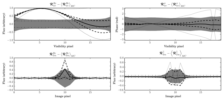
Figure 1: We use Monte-Carlo simulations to study the ability of the Unscented Transform to properly describe the data statistics after the non-linear measurement operator and the different representation operators $\bm{\mathcal{R}}$ (Sec. 3.1) have been applied to the process domain. Here we consider the case of a frequency-dependent phase gradient (clock offset, ionospheric effect, or source position offset). We have subtracted the true mean $\left<\bm{\mathcal{R}}\right>_{MC}$ to each quantity plotted in this figure. The true covariance corresponds to the gray area, while the sigma points appear as dotted lines, together with their associated estimated covariance (thick dashed line). The noise in the data is represented by the dash-dotted line. Qualitatively, the goodness of the description depends on the type of the data representations operator.

3 Data representation

In this section we describe how we can modify the measurement operator together with the raw data to improve robustness. Using the operator discussed in Sec. 3.2 in combination with the Kalman filter discussed above, this is equivalent to an image-plane calibration.

3.1 Robustness with large process covariance

As explained in Sec. 2.2 and 4, the Unscented Transform correctly approximates the evolved covariance up to the third order. When the radius of the sphere containing $\sigma$-points in the process domain increase, and depending on the strength of non-linearities of the evolution and measurement operators f and h, the estimated mean and covariance can be affected by large errors. This is the case when the multivariate ellipsoid is too deformed, and the statistics of the $\sigma$-points in the evolved domain do not capture anymore the true statistics.

Here, we introduce another layer of non-linear operators $\bm{\mathcal{R}}:\mathbb{R}^{2M}\mapsto\mathbb{R}^{\tilde{M}}$ that transform the sets of visibilities into another measurement domain. We define various simple representation operators as follows:

$$\bm{\mathcal{R}}^{||}_{\mathrm{Img}}: \mathbb{R}^{2M}\rightarrow\mathbb{R}^{M_{i}} \qquad\bm{\mathcal{R}}^{Re}_{\mathrm{uv}}: \mathbb{R}^{2M}\rightarrow\mathbb{R}^{M}$$

$$\textbf{y}\mapsto\left|\textbf{g}_{\text{1D}}(\textbf{y})\right| \textbf{y}\mapsto Re(\textbf{y})$$

$$\bm{\mathcal{R}}^{\phi}_{\mathrm{uv}}: \mathbb{R}^{2M}\rightarrow\mathbb{R}^{M} \qquad\bm{\mathcal{R}}^{Re}_{\mathrm{Img}}: \mathbb{R}^{2M}\rightarrow\mathbb{R}^{M_{i}}$$

$$\textbf{y}\mapsto\phi(\textbf{y}) \textbf{y}\mapsto Re(\textbf{g}_{\text{1D}}(\textbf{y}))$$

where $\textbf{g}_{\text{1D}}=\bm{\mathcal{R}}^{\mathbb{C}}_{\mathrm{Img}}$ is the operator described in Sec. 3.2 transforming a set of visibilities into another set of 1-dimensional images (the Fourier transform along the frequency axis, also refered later as the pseudo-image domain). The operators $\left|\textbf{.}\right|$, $\phi(\textbf{.})$ and $Re(\textbf{.})$ take the complex norm, the phase and the real part respectively. $M$ is the number of visibility data, $M_{i}$ the number of pixels in the image domain. Our goal is to obtain a system that has less non-linearity, so that the $\sigma$-points statistics still properly match the true statistics, even when the volume within the multivariate ellipsoid is large in the process domain.

In order to illustrate this idea, we compare the evolved covariance estimated using Eq. 19 to the true evolved mean and covariance as estimated by running Monte Carlo simulations. The system is made of one point source at the phase center, the bandpass goes from $30$ to $70$ MHz, and our interferometer consists of one baseline. We consider the ellipsoid of the clock-offset parameter $\Delta t_{01}\sim\mathcal{N}(0,10)\times 10^{-9}\text{s}$ (therefore corresponding to a large $10\times 10^{-9}$ sec. estimated error), and inspect how it is reflected in the data domains after applying $\widetilde{\textbf{h}}=\bm{\mathcal{R}}\circ\textbf{h}$ (the symbol $\circ$ is used here for the function composition). For that system, Eq. 1 becomes $\widetilde{\textbf{y}}=\widetilde{\textbf{h}}(\textbf{x})=\bm{\mathcal{R}}\left(\exp{\left(2\pi i\nu\Delta t_{01}\right)}\right)$, where $\Delta t_{01}$ is our random variable. Fig. 1 shows how the statistics of the $\sigma$-points compare to the true statistics when using different data representations $\bm{\mathcal{R}}$. When $\bm{\mathcal{R}}$ picks the real part $Re$ or the phase $\phi$ of $\textbf{y}=\widetilde{\textbf{h}}(\textbf{x})$ ($\bm{\mathcal{R}}^{Re}_{\mathrm{uv}}$ and $\bm{\mathcal{R}}^{\phi}_{\mathrm{uv}}$), the $\sigma$-points statistics are obviously wrong.

3.2 One-dimensional image domain for calibration

Although a single transformation separate the uv-plane from the image domain, it seems the later is sometimes more suited for calibration. Intuitively, in the uv domain, clock shifts, source position, ionospheric disturbance will wrap the phases of the complex-valued visibilities everywhere, and the strong non-linearities sometimes present in h make the distribution strongly non-Gaussian. On the contrary, in the image domain, the same type of perturbations only affect the data locally, and will move the flux from one pixel to its neighborhood.

We cannot use the 2-dimensional image domain, as it is build from the superposition of all baselines, which would lead to an effective loss of information. Instead, similarly to what is done for VLBI delays and fringe rates calibration (Cotton 1995), we build a 1D image per baseline (see Appendix A for details). As shown in Fig. 1, when going into the pseudo-image domain, the power is concentrated in a few pixels. The real part $\bm{\mathcal{R}}^{Re}_{\mathrm{Img}}$ of individual pixels gives a better match, but is still biased. Taking the norm $\bm{\mathcal{R}}^{||}_{\mathrm{Img}}$ of the image-plane complex pixel seems to behave well in all conditions. This is discussed in detail in Appendix A.

3.3 The augmented measurement state for regularization

As explained above, one of the aim of the work presented in this paper is to address the ill-conditioning issues related to the large inverse problem underlying the use of modern interferometers. This is done by analytically specifying the physics underlying the RIME (using a Physics-based approach - see Sec. 1.1), and by using the Kalman filter mechanism, able to constrain the location of the true process state through the transmission of previous estimated state and associated covariance. Yet, in some situations, and particularly when two variables are analytically degenerate (such as the clock shifts and the ionosphere when the fractional bandwidth is small), the robustness of the scheme presented is not strong enough to guarantee the regularity of solutions, and the estimated process can drift to a domain where solutions are non-physical.

In order to take into account external constrains while still properly evolving the process covariance $\textbf{P}_{k\mid k}$, we introduce an augmented measurement model (see for example Henar 2011; Hiltunen et al. 2011). Using the idea underlying Tikhonov regularization, if $\textbf{x}_{0}$ is the expected value of x, and $\textbf{Q}^{\gamma}_{0}$ the covariance of $\textbf{x}_{0}$, our cost function becomes:

$$\mathcal{C}(\textbf{x}) =\|\widetilde{\textbf{h}}(\textbf{x})-\widetilde{\textbf{y}}\|^{2}_{\textbf{P}}+\|\textbf{x}-\textbf{x}_{0}\|^{2}_{\textbf{Q}^{\gamma}_{0}}$$ (24)

$$=\left\|\left[\begin{array}[]{c}\widetilde{\textbf{h}}(\textbf{x})\\ \textbf{x}\end{array}\right]-\left[\begin{array}[]{c}\widetilde{\textbf{y}}\\ \textbf{x}_{0}\end{array}\right]\right\|^{2}_{(\textbf{P},\textbf{Q}^{\gamma}_{0})}$$ (29)

$$=\|\widetilde{\textbf{h}}^{a}(\textbf{x})-\widetilde{\textbf{y}}^{a}\|^{2}_{(\textbf{P},\textbf{Q}^{\gamma}_{0})}$$ (30)

where $\|\textbf{x}\|_{\textbf{C}}=\textbf{x}^{T}\textbf{C}^{-1}\textbf{x}$, is the norm of vector x for the metric C, with C the covariance matrix of x (or the Mahalanobis distance). The operator $\widetilde{\textbf{h}}^{a}:\mathbb{R}^{N}\mapsto\mathbb{R}^{M+N}$ is the augmented version of h and $(\textbf{P},\textbf{Q}^{\gamma}_{0})$ is the block diagonal covariance matrix of the augmented process vector. The parameter $\gamma$ allows to control the strength of the Tikhonov regularization, and is such that $\textbf{Q}^{\gamma}_{0}=\gamma^{-2}\textbf{Q}_{0}$.

4 Implementation for radio-interferometry

As explained above, radio-interferometry deals with a large inverse problems, made of millions or billions of non-linear equations. This poses a few deep problems including (i) numerical cost and (ii) numerical stability. In this section, we describe our UKF implementation.

4.1 Woodbury matrix identity

The first issue is the size of the matrices involved in the UKF recursion steps presented in Sec. 2.2. Specifically, in the case of LOFAR, we have $n_{bl}\sim 1500$ baselines and $n_{\nu}\sim 250$ frequencies. This gives a number of dimensions $M$ for the measurement space of $M\sim 1.5\times 10^{6}$ per recursion (taking into account the 4-polarization visibilities). The predicted measurement covariance matrix $\textbf{P}_{y_{k}y_{k}}$ has size $M\times M$, and in practice becomes impossible to store and invert directly ($\sim 8$ Peta-bytes of memory). Fortunately we can re-factor Eq. 21 so that we do not have to explicitly calculate each cell of $\textbf{P}_{y_{k}y_{k}}$. We can see that Eq. 19 can be rewritten as

$$\textbf{P}_{y_{k}y_{k}} = \ \textbf{S}_{k}\textbf{W}\textbf{S}_{k}^{T}+\textbf{R}_{k}$$ (31)

with $$\begin{cases}[\textbf{S}_{k}]_{i}&=\ \bm{\mathcal{Y}}_{k}^{i}-\hat{\textbf{y}}_{k}\\ \textbf{W}_{ij}&=\begin{cases}w^{c}_{i}&\qquad\text{if}\ i=j\\ 0&\qquad\text{otherwise}\\ \end{cases}\end{cases}$$

where $\textbf{S}_{k}$ is a matrix of size $M\times(2N+1)$, $[\textbf{S}_{k}]_{i}$ is the $i^{th}$ column of $\textbf{S}_{k}$, and W is a diagonal matrix of size $(2N+1)\times(2N+1)$ containing the weights on its diagonal. Using the Woodbury matrix identity (Hager 1989), we can express the Kalman gain $\textbf{K}_{k}$:

$$\textbf{K}_{k} =\textbf{P}_{x_{k}y_{k}}\textbf{P}_{y_{k}y_{k}}^{-1}$$

$$=\textbf{P}_{x_{k}y_{k}}\textbf{R}_{k}^{-1}\left(\textbf{I}-\textbf{S}_{k}\left(\textbf{W}^{-1}+\textbf{S}_{k}^{T}\textbf{R}_{k}^{-1}\textbf{S}_{k}\right)\textbf{S}_{k}^{T}\textbf{R}_{k}^{-1}\right)$$ (32)

This relation (Eq. 4.1) is quite remarkable, as it allows us to apply the Kalman gain without explicitly calculating it, and without estimating $\textbf{P}_{y_{k}y_{k}}$ and its inverse either. Instead, the inverse $\textbf{W}^{-1}$ of the diagonal weight matrix of size $(2N+1)\times(2N+1)$, and the inverse $\textbf{R}_{k}^{-1}$ of the data covariance matrix of size $M\times M$ have to be estimated. Even though $\textbf{R}_{k}$ has large dimensions, if the noise is uncorrelated only the diagonal has to be stored and the inverse can be computed element-by-element. Similarly, inner product of matrices with $\textbf{R}_{k}$ are computationally cheap. At each recursion $k$ we have to explicitly estimate the $\sigma$-points evolved through the measurement operator h and contained in $\textbf{S}_{k}$.

4.2 Adaptive step

While $\textbf{P}_{k\mid k}$ characterizes the posterior process covariance, the matrix Q (Eq. 4 and 16) characterizes the intrinsic process covariance through time. It can for example describe the natural time-variability of the ionosphere, the speed of the clock drift, or the beam stability. In addition, in strong non-linear regime, it is well known that the Kalman filters can underestimate $\textbf{P}_{k\mid k}$, and thereby drive biases in the estimate $\hat{\textbf{x}}_{k\mid k}$ of $\textbf{x}_{k}$. This would typically happen when $\hat{\textbf{x}}_{k-1\mid k-1}$ is too far from x, or when the process covariance is changing (for example a changing and increasing ionospheric disturbance for a given time-period). Although the Kalman filter does not produce an update $\textbf{Q}_{k}$ of Q, based on the residual data we can externally update it and write $\textbf{Q}_{k}=\kappa\textbf{Q}$. The scaling factor $\kappa$ is useful to estimate whether the model is properly fitting the data at any time step $k$. Following Ding et al. (2007), we can write:

$$\kappa = \sum\limits_{i}w^{i}_{\textbf{Q}}\frac{\operatorname{tr}\left\{(\textbf{y}_{k-i}-\hat{\textbf{y}}_{k-i})(\textbf{y}_{k-i}-\hat{\textbf{y}}_{k-i})^{T}-\textbf{R}_{k-i}\right\}}{\operatorname{tr}\left\{\textbf{S}_{k-i}\textbf{W}\textbf{S}_{k-i}^{T}\right\}}$$ (33)

$$w^{i}_{\textbf{Q}} = \exp{\left(-(t_{k}-t_{k-i})/\tau_{\textbf{Q}_{k}}\right)}$$ (34)

where $\operatorname{tr}\left\{\textbf{A}\right\}$ is the operator computing the trace of a matrix A. The weights are designed to take into account past residual values, and $\tau_{\textbf{Q}_{k}}$ is a time-type constant. Here, estimating $\kappa$ is computationally cheap as $\operatorname{tr}$ only accesses the diagonal of the input matrix.

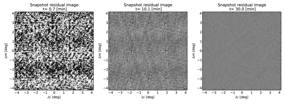
Figure 2: This figure shows the snapshot residual image estimated at different recursion times (the color scale is identical in each panel). As recursion time evolves, more data have “crossed” the Kalman filter, the ionospheric and clock parameters estimates are getting more accurate, and the residual noise level decreases (see also Fig. 4).

4.3 Computational cost

In this section, we discuss the computational cost of the proposed algorithm. Our concern is to show that the approach is feasible, and we do not intend to show that it is faster than other existing approaches. However, we discuss the issues of the scaling relations and parallelizability of various parts of the algorithm. We argue that using the refactorization described in Sec. 4.1, our algorithm should be compatible with existing hardware, even for the datasets produced by the most modern radiotelescopes.

As explained above, we adopt a Physics-based approach to reduce the number of degrees of freedom by orders of magnitudes while using more data at a time (see Sec. 1.1 for a discussion on Jones-based versus Physics-based approach). The Kalman filter is fundamentally recursive (i.e. it has only one iteration), while tens to hundreds of iterations are needed to reach local convergence with Levenberg-Marquardt for example. This means that the equivalent gain by the proposed approach on the model estimation side is the number of iteration. This gain might be balanced in some cases by the larger data chunks processed at a time by the Kalman filter itself. We give here the scaling relations for our implementation of the filter scheme.

The predict step (controlled by operator f in Sec. 2.2) always represents a relatively small number of steps, as it scales with the number of parameters $N$ in the process vector. The update step however is the costly part of the computation (Sec. 2.2). It consists of (i) estimating the data corresponding to different points in the process domain (applying the operator h, see Eq. 1) and (ii) computing the updated estimate of the process vector and associated covariance. Step (i) is common to all calibration algorithms, and in the majority of cases this is the expensive part of the calculation as we map $N$ parameters to $M$ data points, $M$ having relatively high values of $\sim 10^{4}-10^{6}$. Indeed, within our framework, most of the computation is spent in the estimate of $\textbf{S}_{k}$ of size $M\times(2N+1)$ (Eq. 17), which, compared to the Jacobian equivalent that would have size $M\times N$, represents a cost of a factor of $\sim 2$ in computational cost. It is worth to note that this step is heavily parallelisable. The series of operation in (ii) to apply the Kalman gain (Eq. 4.1) are negligible in terms of computing time for the example described in Sec. 5.1. From the scaling associated with the use of the Woodbury matrix identity, following the work presented in Mandel (2006), we estimate this operation should scale as $\mathcal{O}(N^{3}+MN^{2})$.

We believe the algorithm should be practical with large datasets. For the few test cases we have been working on (with a 4-core CPU) with $\sim 20$ to $\sim 100$ parameters, and moderate to large dataset (such as the LOFAR HBA dataset containing $\sim 1500$ baselines, 30 sub-bands, and a corresponding $M\sim 1.8\times 10^{5}$ points per recursion, see Sec. 5.1.2), the algorithm was always faster than real time by a factor of several. On the LOFAR CEP1 cluster, a distributed software would work with up to $M\sim 10^{6}$ points per recursion and $N\sim 100$. Preliminary tests showed that the Kalman filter most consuming steps appearing in Eq. 4.1 are computed within a few seconds (computing inner products with numpy/ATLAS, on an 8-core CPU).

5 Simulations

In this section, we present simulations for (i) the pointing error calibration problem (also addressed using Physics-based algorithms in Bhatnagar et al. 2004; Smirnov 2011) and (ii) the clock/ionosphere problem.

5.1 Clock drifts and ionosphere

LOFAR raw datasets are characterized by a few dominating direction-independent and direction-dependent effects, including clocks and ionosphere. While direction dependent calibration is known to be difficult, clock errors and ionosphere effects combined with a limited - even though large - bandwidth make the problem partially ill-conditioned.

5.1.1 Evolution and Measurement operators

The error $\delta t^{\mathrm{clk}}_{p}$ due to the clock offset of antenna $p$ produce a linearly frequency-dependent phase $\phi^{\mathrm{clk}}_{p}=2\pi\nu\delta t^{\mathrm{clk}}_{p}$. The time delay $\delta t_{p,d}^{\mathrm{ion}}$ introduced by the ionosphere is frequency dependent $\delta t_{p,d}^{\mathrm{ion}}\propto T_{p,d}/\nu^{2}$, where $T_{p,d}$ is the Total Electron Content (TEC), given in TEC-units (TECU), and seen by station $p$ in direction $d$. This gives a phase $\phi_{p,d}^{\mathrm{ion}}=kT_{p,d}/\nu$, with $k=8.44\times 10^{9}$ m³.s^-2.

The measurement operator h (Eq. 1) is built from the direction independent $\textbf{G}_{pt\nu}$ and direction dependent terms $\textbf{D}^{d}_{pt\nu}$ as follows:

$$\textbf{G}_{pt\nu}(\textbf{x}) := \exp\left(2\pi i\nu\ \delta t_{p}(\textbf{x})\right)\textbf{I}$$ (35)

$$\textbf{D}^{d}_{pt\nu}(\textbf{x}) := \exp\left(ik\nu^{-1}\ T^{d}_{p}(\textbf{x})\right)\textbf{I}$$ (36)

where I is the $2\times 2$ unity matrix, $\delta t_{p}$ is a simple linear operator unpacking the clock value of antenna $p$ from the process vector x. For this test, we choose to model the ionosphere using a Legendre polynomial function (see for example Yavuz 2007). Assuming a single ionospheric screen at a height of $100$ km, the non-linear operator $T^{d}_{p}$ extracts the Legendre coefficients, and returns the TEC value seen by antenna $p$ in direction $d$. For this simulation, we are using the $\bm{\mathcal{R}}^{||}_{\mathrm{Img}}$ representation presented in Sec. 3.

The operator f describing the dynamics of the system typically contains a lot of physics. Clock offsets drift linearly with time, while the ionosphere has a non-trivial behaviour (defined in Sec. 5.1.2). We configure the filter to consecutively use two types of evolution operator f. The first is used for the first $\sim 6$ minutes, and f is the identity function, which corresponds to a stochastic evolution. This appears useful when the initial process estimate starts far from the true process state. This way, the filter’s state estimate get closer to the true state without assuming any physical evolutionary dynamics. The convergence speed and accuracy are then both controlled by the covariance matrices $\textbf{P}_{k}$ and $\textbf{Q}_{k}$ described above. We set the second evolutionary operator f to be an extrapolating operator. It computes an estimated process vector value from the past estimates. At time step $k$, for the $i^{th}$ component of x, solutions are estimated as follows:

$$\textbf{f}(\textbf{x}^{i}_{k}) := \bm{\mathcal{P}}\left(\{\textbf{x}_{k-m}\},n^{i}_{\mathrm{fit}},\tau_{i}\right)$$ (37)

$$w^{i}_{t-m} = \exp{\left(-(t_{k}-t_{t-m})/\tau_{i}\right)}$$ (38)

where $\bm{\mathcal{P}}$ is the operator computing the polynomial interpolation, $n^{i}_{\mathrm{fit}}$ is the degree of the polynomial used for the interpolation, $w_{i}$ are the weights associated with each point $\textbf{x}_{k-m}$ at $t_{k-m}$, and $\tau_{i}$ gives a time-scale beyond which past information is tapered.

5.1.2 Simulation for LOFAR

An important consideration is that at any given time our algorithm needs to access all frequencies simultaneously. With $250$ sub-bands ($16$-bit mode), $1$ channel per sub-band, $1500$ baselines, $4$ polarization, this gives a number of visibilities per recursion of $1.5\times 10^{6}$. The data is currently distributed and stored per sub-band - so our software needs to deal with a number of technical issues for a realistic full size simulation. For this simulation, we scale down the problem by a factor $\sim 8$ in terms of number of frequency points per recursion. Assuming NVSS source counts (Condon et al. 1998), a spectral index of $-0.8$, and a field of view of $8$ degrees in diameter, we estimate a total of $\sim 20$ Jy of signal per pointing at $\sim 150$ MHz. Inspecting the cross polarizations visibilities of a LOFAR calibrated data-set with $\Delta\nu=0.2$ MHz and $\Delta t=6$ s gives an estimated noise of $\sim 2$ Jy per visibility bin. We work on $30$ sub-bands only, with frequencies linearly distributed between $100$ and $150$ MHz, and scale the signal to match $\mathrm{SNR}\sim 10$ per visibility per sub-band. We distribute the corresponding flux density on a $3\times 3$ rectangular grid of sources with a step of $3$ degrees in RA and $3$ degrees in DEC.

For the dynamics of the underlying physical effects, we apply a linearly drifting clock offset taken at random with $\partial(\delta t^{\mathrm{clk}}_{p})/\partial t\sim\mathcal{N}(0,10)$ ns. As mentioned above we model the ionosphere with a 2D-Legendre polynomial basis function. For this simulation, each Legendre $l_{ij}$ coefficients varies following $l_{ij}=\sin(t/\tau_{ij}+d\tau_{ij})$, with $\tau_{ij}$ and $d\tau_{ij}$ taken at random. Along these lines discussed above, we set $(n^{i}_{\mathrm{fit}},\ \tau_{i})=(1,\ 5\text{min})$ and $(n^{i}_{\mathrm{fit}},\ \tau_{i})=(2,\ 1\text{min})$ for the clock and for the ionosphere respectively. These orders for the extrapolating polynomials are in agreement with the linear clock drift, and the non-linear behaviour of the ionosphere.

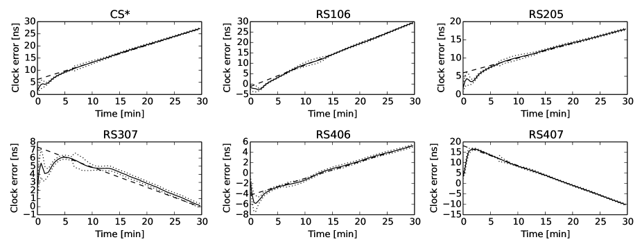
Figure 3: This figure shows the estimated clock errors (full line) as well as the posterior covariance (dotted line) as a function of time for different LOFAR stations in the simulation presented in Sec. 5.1. The dashed line shows the true underlying clock offset. In order to improve convergence speed, before $t=6$ min. the evolutionary model is stochastic.

5.1.3 Results

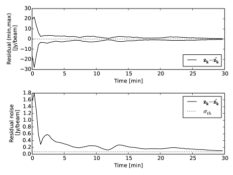
Figure 4: Top panel shows the maximum and minimum residual values in the snapshot image as a function of recursion time (full line). In the bottom panel we plot the standard deviation in the residual snapshot maps. The expected thermal noise is shown in the bottom figure as the dotted line.

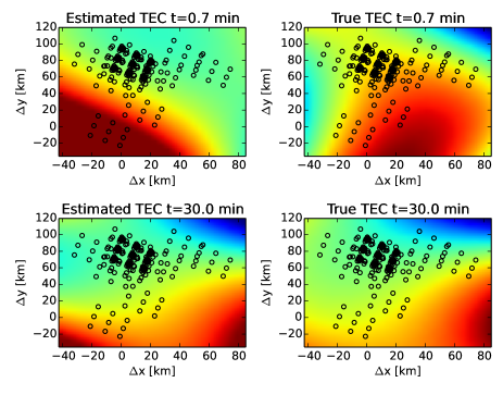
Figure 5: The ionosphere state is described using a Legendre polynomial basis function. We show here the estimated and true state of the ionosphere (left and right panels), at the beginning and at the end of the filter’s recursion. The open circles show the location of the pierce points in the ionosphere. The spacial coordinates are given in kilometers from the array center projected on the ionosphere screen.

The filter and simulation configuration are described in Sec. 5.1.1 and 5.1.2 respectively. At each recursion step, $\sim 180.000$ complex visibilities “cross” the filter and the process state (clock and ionosphere) as well as its covariance are estimated.

First, in order to inspect the match to the data we derive the frequency-baseline-direction dependent Jones matrices at the discrete locations of the sources in our sky-model, and subtract the visibilities corresponding to the given discrete directions. We then grid the residual visibilities and compute the snapshot images (see Fig. 2). Fig. 4 shows the minimum and maximum residual as well as the standard deviation as a function of time. Very quickly the visibilities are correctly matched down to the thermal noise.

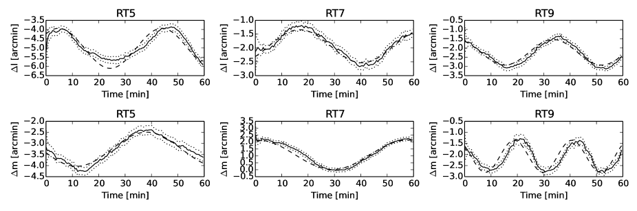
Figure 6: This figure shows the true pointing errors for a WSRT simulation (dashed line) together with the estimated state as a function of time (full line). Our algorithm properly tracks the time dependent pointing errors within the estimated covariance (dotted line).

In Fig. 3 we show the clock offsets estimates as a function of time, as compared to the true clock errors. The clock offsets estimates seem to converge asymptotically to the true underlying states. The ionospheric parameter estimates are more subject to ill-conditioning, as some parts of the TEC-screen are not pierced by any projected station. However, plotting the TEC-screen corresponding to the individual Legendre coefficients gives a good qualitative match to the true TEC values (Fig. 5).

5.2 Pointing errors

One of the dominating calibration errors for interferometers using dishes are the individual antenna pointing errors. They start to have a significant effect even at moderate dynamic range, and can be severe for non-symmetric primary beams with azimuthal dish mounts. Bhatnagar et al. (2004) and Smirnov (2011) have presented a Physics-based calibration scheme to specifically solve for pointing errors, using a least-squares minimization technique combined with a beam model.

Here, we simulate a Westerbork Synthesis Radio Telescope (WSRT) data-set. As in Sec. 5.1, we first define a measurement equation (operator h). We only consider the direction dependent primary beam effect, using the WSRT $\cos^{3}$ beam model:

$$\textbf{G}_{pt\nu}(\textbf{x}) :=$$ I (39)

$$\textbf{D}^{d}_{pt\nu}(\textbf{x}) := \cos\left(\min\left\{65\ [\nu/10^{9}]\ r^{d}_{pt}(\textbf{x}),1.0881\right\}\right)^{3}\textbf{I}$$ (40)

$$r^{d}_{pt}(\textbf{x}) = \sqrt{(l^{d}-\delta l_{pt}(\textbf{x}))^{2}+(m^{d}-\delta m_{pt}(\textbf{x}))^{2}}$$ (41)

where $\delta l_{pt}$ and $\delta m_{pt}$ are the operators unpacking the pointing errors values $\delta l$ and $\delta m$ for antenna $p$ at time $t$. The f evolution operator is the same as in Sec. 5.1.1, with $\tau_{i}=5$ min (Eq. 37). We simulate a data-set containing $64$ channels centered at $\sim 1.3$ GHz and channel width $\delta\nu=0.3$ MHz. The sky model has $20$ sources with a total flux density of $\sim 10$ Jy, with a noise of $0.2$ Jy per visibility. The simulated pointing errors have an initial global offset distributed as $\delta l_{0}\sim\delta m_{0}\sim\mathcal{N}(0,3)$ arcmin, and the pointing offsets evolve periodically as $\delta l(t)=l_{0}+a_{l}\cos(2\pi t/\tau_{l}+\phi_{l})$, with $a_{l}\sim\mathcal{N}(1,0.3)$ arcmin, $\tau_{l}\sim\mathcal{N}(40,10)$ min, and $\phi_{l}$ uniformly distributed between $0$ and $2\pi$. The same scheme is used to generate the evolution law for $\delta m$).

Fig. 6 shows the comparison between the estimated pointing errors are the true pointing errors for a few antennas. The filter’s estimate rapidly converges to the true pointing offset, and properly tracks its state within the estimated uncertainty.

6 Discussion and conclusion

6.1 Overview: pros, cons and potential

As discussed throughout this paper, it is important to obtain robust algorithms that do not affect the scientific signal. In this paper, we have presented a method that aims at improving robustness along the following lines:

1. The Kalman filter presented here is fundamentally recursive, and information from the past is transferred along the recursion, thereby constraining the expected location of the underlying true state. This is fundamentally different from minimizing a least square, and then smoothing or interpolating the solution - especially since we can assume a physical measurement and evolutionary model.

2. Contrarily to the Jones-based algorithms that have to deal with hundreds of degrees of freedom, our algorithm follow a Physics-based approach (see in Sec. 1.1 for other Physics-based methods). It aims at estimating the true underlying physical term, potentially describing the Jones matrices of individual effects everywhere in the baseline-direction-frequency space. The very inner structure of the Radio Interferometry Measurement Equation (RIME) can be used to constrain the solutions. This feature allows us to take into account much bigger data chunks. Typically, most effects have a very stable frequency behaviour, and the data in the full instrumental bandwidth can be simultaneously used at each recursion. This improves conditioning.

3. The measurement operator is non-linear, and combining (a) with (b) is made possible by using a modern non-linear version of the Kalman filter, together with the representation operator presented in Sec. 3.

4. Ill-conditioning can still be significant if effects are analytically degenerate to some degree. We can modify the measurement operator to take external prior information into account (see Sec. 3.3), and reject solutions that are considered to be non-physical. For example, this can allow the user to provide the filter with an expected ionospheric power spectrum of the Legendre coefficients.

5. One of the benefits of using filters is that they produce a posterior covariance matrix on the estimated process state. The covariance estimate should be reliable assuming the non-linearities are not too severe.

Given the large size of our inverse problem, and in order to make any algorithm practical, optimizing the computational cost is of prime importance. Using the Woodbury matrix identity (Sec. 4.1), we re-factor the Unscented Kalman Filter steps to make the algorithm practical. Even for the moderately large simulations described in Sec. 5.1, a 4-core CPU is able to constrain solutions faster than real time. The need to access the data of all frequencies simultaneously represents some technical problems, as these are distributed over different cluster nodes.

An important potential problem with Physics-based approaches is that the system needs to be described analytically, while algorithms solving for the effective Jones matrices do not use any assumptions about the physics underlying the building of a visibility (apart from the sky model that is assumed). This would cause problems in particular if the model encapsulated in the operator h misses physical ingredients that are present in reality, and would probably drive biases in the estimates. Furthermore, the Unscented Kalman Filter used and adapted to the context of radio-interferometry in this paper deals with non-linearities only up to a certain level. This means in practice that the process a priori covariance has a certain maximum size, for a given type of non-linearities.

6.2 Conclusion

The use of filters and similar methods can potentially improve radio interferometric calibration. As with least squares minimization techniques, our approach is guaranteed to work only if non-linearities are not too severe in the neighborhood of the true process state. Other algorithms dealing with non-linearities are known to provide higher robustness, such as more general particle filters, or Monte-Carlo Markov Chains. The later is indeed guaranteed to provide a correct estimated posterior distribution. However, most of these methods are expensive because of the many predict steps that have to be computed, and this fact could make them impractical, given the large size of our problem. Recursive algorithms are well adapted to streaming pre-calibration, and based on preliminary simulations, our algorithm seems to be robust enough to solve for the sky term (positions, flux densities, spectral indices, etc.) in a streaming way.

We have not yet demonstrated the efficiency of our algorithm with real datasets essentially because of its complexity and novelty. Indeed, our software needs to deal with a number of technical issues as well as more fundamental problems. Specifically in the case of the newest interferometers such as LOFAR, (i) we have to deal with large quantities of distributed data, and the algorithm has to access all frequencies simultaneously. Beyond these technical aspects, because we solve for the underlying physical effects, (ii) we need to build pertinent physical models for the various effects we are solving for, such as ionosphere, or phased array beams. An application of this algorithm to real datasets will be presented in a future paper.

Appendix A One-dimensional images properties

In this section we discuss in more detail the one-dimensional image representations introduced in Sec. 3. Aiming at being as conservative as possible, but still working in the image domain, we define $\textbf{g}_{\text{1D}}$ to be the operator that builds one 1D image per baseline $(pq)$, and polarization $i$ as:

$$\widetilde{\textbf{y}}_{(pq),i} =\textbf{g}_{\text{1D}}(\textbf{y}_{(pq),i})$$

$$:=\int_{-\infty}^{\infty}\textbf{y}_{(pq),i}(\nu)\ \exp\left(2\pi i\frac{\nu}{\text{c}}\textbf{b}_{pq}^{T}\textbf{s}\right)d\nu$$

$$=\int_{-\infty}^{\infty}\textbf{V}_{(pq),i}(\nu)\ \mathrm{rect}\left(\frac{\nu-\nu_{m}}{\Delta\nu}\right)\exp\left(2\pi i\frac{\nu}{\text{c}}\textbf{b}_{pq}^{T}\textbf{s}\right)d\nu$$ (42)

$$\text{with }\textbf{V}_{(pq),i} =\sum_{d=1}^{n_{d}}\text{S}^{d}_{i}\exp\left(-2\pi i\frac{\nu}{\text{c}}\textbf{b}_{pq}^{T}\textbf{s}_{d}\right)d\nu$$ (43)

where $c$ is the speed of light, $\mathrm{rect}$ is the rectangular function, $\nu_{m}=(\nu_{0}+\nu_{1})/2$, $\Delta\nu=\nu_{1}-\nu_{0}$ with $\nu_{0}$ and $\nu_{1}$ the minimum and maximum available frequencies. In order to align the $u$-coordinate with the frequency extent of the baseline, we rotate $\textbf{b}_{pq}$ and s and $\textbf{s}_{d}$ with $3\times 3$ rotation matrix $\textbf{U}_{\theta\phi}$ such that:

$$\textbf{b}_{\theta\phi} =\textbf{U}_{\theta\phi}\left[\begin{array}[]{c}u_{pq}\\ v_{pq}\\ w_{pq}\end{array}\right] =\left[\begin{array}[]{c}u_{pq}^{\prime}\\ 0\\ 0\end{array}\right]$$ (50)

$$\textbf{s}_{\theta\phi} =\textbf{U}_{\theta\phi}\left[\begin{array}[]{c}l\\ m\\ n-1\end{array}\right] =\left[\begin{array}[]{c}l^{\prime}\\ m^{\prime}\\ n^{\prime}\end{array}\right]$$ (57)

where $(l,m,n)$ are the image plane coordinates, $(u_{pq},v_{pq})$ are the uv-coordinate of baseline $(pq)$, $(\nu_{0},\nu_{1})$ are the lower and higher frequencies values of the interferometer’s bandpass. It is unitary so $\textbf{b}^{T}\textbf{s}=\textbf{b}_{\theta\phi}^{T}\textbf{s}_{\theta\phi}$. We can write the complex 1-dimensional image as:

$$\widetilde{\textbf{y}}_{(pq),i} =\sum_{d=1}^{n_{d}}\text{S}^{d}_{i}\delta({l^{\prime}_{d}})*\text{PSF}_{1D}$$ (58)

where $*$ is the convolution product, $\text{S}_{d,i}$ is the apparent flux of the source in direction $d$ for polarization $i$.

More intuitively, this means that $\widetilde{\textbf{y}}_{(pq),i}$ is obtained by projecting the sky on the baseline, and convolving it with the 1-dimensional PSF of the given baseline. The term $\text{PSF}_{1D}$ is obtained by computing the inverse Fourier transform of the uv-domain sampling function:

$$\text{PSF}_{1D}(l^{\prime}) =\mathcal{F}^{-1}\left\{\mathrm{rect}\left(\frac{\nu-\nu_{m}}{\Delta\nu}\right)\right\}$$ (59)

$$=\textrm{sinc}\left(u^{\prime}\Delta\nu l^{\prime}/c\right)\exp{\left(2\pi iu^{\prime}\nu_{m}l^{\prime}/c\right)}$$ (60)

where sinc is the cardinal sine function. We can see in Eq. 60 that $\text{PSF}_{1D}$ contains both low and high spacial frequency terms ($u^{\prime}\Delta\nu/c$ and $u^{\prime}\nu_{m}/c$ respectively, whose ratio equals the fractional bandwidth).

Therefore, while $\bm{\mathcal{R}}^{Re}_{\mathrm{Img}}$ still contains the high frequency fringe, taking the complex norm using $\bm{\mathcal{R}}^{||}_{\mathrm{Img}}$ eliminates the high spacial frequency term, and $\text{PSF}_{1D}$ under $\bm{\mathcal{R}}^{||}_{\mathrm{Img}}$ is smoother ($\bm{\mathcal{R}}^{Re}_{\mathrm{Img}}$ extracts the envelope of $\text{PSF}_{1D}$). This intuitively explains why the $\bm{\mathcal{R}}^{||}_{\mathrm{Img}}$ representation seems to provide a better match between the true and the $\sigma$-points statistics. As the clock and ionospheric displacements mostly amount to apparent shifts in source locations, smoothness of $\bm{\mathcal{R}}^{||}_{\mathrm{Img}}$ provides stability in the $\sigma$-points statistics in the data domain.

Applying any of the representation operators presented above modifies the properties of the input data covariance matrix $\textbf{R}_{k}$ (Eq. 5, 19, and 31). Assuming the noise in the visibilities is uncorrelated, $\textbf{R}_{k}$ is diagonal matrix. Assuming the noise is not baseline or frequency dependent we have $\textbf{R}_{k}=\sigma^{2}\ \bm{\mathcal{I}}$, for $\bm{\mathcal{R}}^{\mathbb{C}}_{\mathrm{uv}}$ and $\bm{\mathcal{R}}^{Re}_{\mathrm{uv}}$, and $\textbf{R}_{k}=(\sigma^{2}/n_{\nu})\ \bm{\mathcal{I}}$ for $\bm{\mathcal{R}}^{Re}_{\mathrm{Img}}$. The statistics of $\bm{\mathcal{R}}^{||}_{\mathrm{Img}}$ are non-Gaussian since it is the norm of a complex number. The random variable is in that case $X=\sigma^{-1}\sqrt{n_{\nu}}\sqrt{(Re^{2}+Im^{2})}$ which follows a non-central $\chi$-distribution with 2-degrees of freedom, and mean and covariance:

$$\mu_{X} =\sqrt{\frac{\pi}{2}}L_{1/2}^{0}\left\{\frac{-\lambda^{2}}{2}\right\}$$ (61)

$$\sigma_{X}^{2} =2+\lambda^{2}-\mu_{X}^{2}$$ (62)

$$\text{with }\lambda =\sqrt{n_{\nu}}\sigma^{-1}\sqrt{\mu_{Re}^{2}+\mu_{Im}^{2}}$$ (63)

where $L_{1/2}^{0}$ is a generalized Laguerre polynomial.