Topological determinants of self-sustained activity in a simple model of excitable dynamics on graphs

Abstract

Models of simple excitable dynamics on graphs are an efficient framework for studying the interplay between network topology and dynamics. This subject is a topic of practical relevance to diverse fields, ranging from neuroscience to engineering. Here we analyze how a single excitation propagates through a random network as a function of the excitation threshold, that is, the relative amount of activity in the neighborhood required for an excitation of a node. Using numerical simulations and analytical considerations, we can understand the onset of sustained activity as an interplay between topological cycle statistics and path statistics. Our findings are interpreted in the context of the theory of network reverberations in neural systems, which is a question of long-standing interest in computational neuroscience.

I Introduction

The diverse ways, in which architectural features of neural networks can facilitate sustained excitable dynamics, is a topic of interest both in the theory of complex networks and in computational neuroscience. Minimal mathematical models can help to understand the generic features of how such dynamics organize on graphs. Here we discuss a simple numerical experiment, where we insert a single excitation into a graph and allow it to propagate with a neuron-like discrete, relative-threshold excitable dynamics. This numerical experiment can be seen as an in vitro setup of signal propagation and amplification. In particular, it serves as a strategy for probing the mechanisms controlling the onset of self-sustained activity in neuronal dynamics. The existence of stable regimes of sustained network activation is an essential requirement for the representation of functional patterns in complex neural networks, such as the mammalian cerebral cortex. In particular, initial network activations should result in neuronal activation patterns that neither die out too quickly nor rapidly engage the entire network. Without this feature, activation patterns would not be stable, or would lead to a pathological excitation of the whole brain. Narrowing down the complex interplay of topology and dynamics to a minimal model scenario allows us to understand microscopically, and to some extent also analytically, the emergence of long transients and, subsequently, self-sustained activity in networks.

In the present study, several topological determinants of sustained activity are characterized and their range of application is delineated. We introduce the concept of barriers, which are topological features possibly disrupting excitation propagation. We analyze the contribution of topological cycles, disrupting the layer-wise excitation fronts, as soon as excitation ‘holes’ (corresponding to high-degree nodes that have not reached the excitation level) start appearing in such fronts. In particular, we propose a mechanistic understanding of some features of the response curve (i.e. the number of successful excitation propagation events as a function of the relative threshold $\kappa$): transition values of $\kappa$ and levels reached by the successful propagation events. This in turn allows a quantitative prediction of these features from the detailed knowledge of the network topology.

The transient sustained activity seen in our excitable model is reminiscent of a biological phenomenon termed network reverberation, that is, the temporarily sustained activity induced by a specific stimulation of a neural circuit. The concept is related to the concept of neural assemblies introduced by Hebb hebb1949 . The intuitive application of such reverberations lies in dynamic memory circuits, that is, online (working) memory based on dynamic patterns, rather than long-term memory that may be encoded in the synaptic weight distribution of the network. Indeed, one can see transiently sustained activity in specific cortical regions (e.g., prefrontal and posterior parietal cortex) related to working memory tasks, such as a delayed matching-to-sample task. The predominant idea is that reverberations are expressed as dynamic attractors of transiently stable increased activity, particularly due to locally increased synaptic strength Wang:2001wk . This idea also provides a link between the dynamic patterns encoding short-term (working) memory and the synaptic weight changes underlying long-term memory. However, there exists an extensive debate on the specific circuitry and parameters underlying the reverberations, e.g. HadipourNiktarash:2003gx ; Muresan:2007ez ; Tegner:2002bc .

Using discrete dynamical models to explore relationships between network architecture and dynamics has provided some key insights into the functions of complex networks in the past, e.g. Boolean models for gene regulatory networks bornholdt2005systems and SIR and SIS models for epidemic diseases in social networks pastor2001epidemic .

How network topology can facilitate the self-sustainment of excitable dynamics on graphs is a fundamental question about the organization of dynamics on graphs roxin04 ; Deco:2009p6486 ; Deco:2011p775 ; ptrs2014 . The role of cycles in excitable dynamics on graphs has received a remarkable amount of attention in the last years Qian:2010a ; Mcgraw:2011jr ; liao:2011 , in particular in Computational Neuroscience lewis2000 ; vladimirov . Cycles have been implicated in maintaining activity in a network vladimirov ; Mcgraw:2011jr . In Garcia:2012ey ; Qian:2010b this role of cycles in graphs has been compared to spiral waves in spatiotemporal pattern formation (see also ptrs2014 ), as the cycle length (similarly to the size of the spiral core) needs to match the refractory period of the excitable units. In garcia2014 it has furthermore been shown that, counterintuitively, the successful usage of long cycles contributes to the sustainment of activity in a graph.

Here our focus is not on cycle usage, but rather on the initial perturbations of the coherent propagating wave front that subsequently leads to the activation of cycles and the onset of sustained activity. Again resorting to the analogy to spatiotemporal pattern formation, we are here exploring the transition from target waves to spiral waves triggered by some heterogeneity in the system. In our case, the source of this heterogeneity is complex network topology.

The respective influence of hubs (high-degree nodes) and modules in shaping activation patterns has been investigated with a focus on the discriminating interplay with spontaneous excitations MullerLinow:2008ia ; hutt2009interplay . The role of cycles in storing excitations and favoring self-sustained activity has been yet elucidated only in a deterministic model of excitable neural networks Garcia:2012ey . A phenomenon of stochastic resonance (noise-facilitated signal propagation) has been evidenced in so-called ‘sub-threshold’ networks, that is, for which a single input excitation does not propagate to the output nodes hutt2012stochastic . However, knowing that there a limit to propagation at some transition value of the parameter $\kappa$ of the excitable dynamics, henceforth denoted $\kappa_{c}$, is not sufficient: it is now necessary to understand what controls the onset or failure of excitation propagation and how the network itself produces such a threshold behavior.

Our principal goal is to gain a mechanistic understanding of the main dynamical processes underlying the two thresholds. For this investigation we employ a discrete-time three-state model of excitable dynamics already used in MullerLinow:2006ex ; MullerLinow:2008ia ; hutt2009interplay ; hutt2012stochastic for analyzing the relationship between network topology and excitable dynamics.

Such cellular automata on graphs are a well established method for probing the relationship between network architecture and dynamics (see, e.g., Li:1992td ; Marr:2030p1915 ; marr2012 ). It is clear that discrete models need to be used with a certain care, as some dynamical effects can indeed be artifacts of the (time and state) discretizations. However, the possibility to unambiguously define events like co-activation or sequential activation make such discrete models powerful tools for exploring the mechanisms by which network architecture dictates some key features of excitable dynamics (see, e.g., Garcia:2012ey ; messe2014 ).

Finding a suitable balance between realism and genericity in modeling excitable dynamics is an important question in computational neuroscience (see, e.g., Giaquinta:2000vg ; Deco:2011p775 ; Garcia:2012ey ; messe2014 . We expect, that the mechanisms / processes here identified (underlying the two thresholds) are elementary enough to be universal and independent of the specific model of excitable dynamics. Like in other fields (e.g. epidemic diseases, moreno02 , or gene regulation, bornholdt2005systems ), the minimal model (a three-state cellular automaton on a graph) enables us to extract a few ‘stylized facts’ about the onset of self-sustained activity, by separating the logical organization (both, on the structural and on the functional level) from the physiological details, how this logical organization is implemented.

Our study focuses on a discrete three-state model representing a stylized biological neuron. While it is conceptually similar to an SIR model, our model is different, both in its biological motivation and (due to the SIR infection probability as the key parameter and source of stochasticity) in its dynamical behavior. The remainder of this paper is structured as follows: First, we briefly summarize the mathematical model, as well as our prediction strategy of the excitation propagation failure or amplification encoded in network architecture (Section II). In Section III we describe the generic properties (transition values of the parameter, excitation levels) of the response curve generated by a single inserted excitation, as well as our prediction results for different network architectures. Section IV discusses, how these features arise from an interplay of cycles and paths statistics in networks. Lastly, we summarize the implications of our findings for computational neuroscience.

II Methods

II.1 Details of the numerical experiment

We start our numerical experiment with a single, randomly chosen input node receiving one excitation, and then observe the propagation of excitations to an output node, selected at random from the nodes at the largest distance from the input node.

We use a three-state cellular automaton model of excitable dynamics. Each node can be in an susceptible/excitable ($S$), active/excited ($E$) or refractory ($R$) state. The model operates on discrete time and employs the following synchronous update rules: For a node $i$ with $k_{i}$ neighbors, the transition from $S$ to $E$ occurs, when at least $\kappa k_{i}$ neighbors are active. The parameter $\kappa$ thus serves as a relative excitation threshold. In such a relative-threshold scenario, low-degree nodes are therefore easier to excite (requiring a smaller number of neighboring excitations) than high-degree nodes. In neuroscience, there is some evidence that this is a plausible excitation scenario, as neurons can readjust their excitation threshold according to the input azouz2000dynamic , which typically leads to spike frequency adaptation benda2003universal , and effectively amounts to a relative input threshold. This model has also been investigated in hutt2012stochastic . After a time step in the state $E$ a node enters the state $R$. The transition from $R$ to $S$ occurs stochastically with the recovery probability $p$, leading to a geometric distribution of refractory times with an average of $1/p$.. Initially all nodes are in the susceptible state $S$. The model does not allow spontaneous transitions from $S$ to $E$ (i.e., compared to previous investigations MullerLinow:2006ex ; MullerLinow:2008ia ; hutt2009interplay , the probability $f$ of spontaneous excitations is set to zero). Therefore, the stochasticity of the dynamics is entirely due to the stochastic recovery, controlled by the recovery probability $p$. For $p$=1, we have a deterministic model (similar to the one discussed in Garcia:2012ey ; there, however, a single neighboring excitation was sufficient to trigger transition to $E$, corresponding to $\kappa\rightarrow 0$).

Previous investigations have considered the case of an absolute threshold, where a fixed number (set to one in previous work) of excited neighbors triggers the activation of a susceptible node. They have shown the key role of hubs as organizing centers of the activity MullerLinow:2008ia ; hutt2009interplay . In contrast, for a relative threshold, there is no amplification due to a potentially increased excitability of high-degree nodes. For a given node, there is moreover a balance between a sufficient number of excited neighbors and the number of susceptible neighbors able to propagate the excitation. Overall, the amplification rate at a given node is bounded by $(1-\kappa)/\kappa$.

We recorded the accumulated excitation of one among the output nodes, during a fixed duration $T$, and plot the result as a function of $1/\kappa$, noting that $1/\kappa$ gives the maximal degree a susceptible node can have to be excited by a single excited neighbor. Any node of degree higher than $1/\kappa$ appears as a barrier, that is, a node for which having a single excited neighbor is not sufficient to get excited.

We adopt a layered view (as in hutt2012stochastic ), according to the shortest distance of the nodes to the input node: the first layer contains the neighbors of the input node, the second layer its second neighbors, and the final layer all the possible output nodes.

Hubs are more likely to be located in the first layer, because even if the input node is not a hub, it will point to a hub with a large probability. Using this layered view is furthermore motivated by the fact that, due to the refractory period, excitation propagates layer-wise at low enough $\kappa$.

II.2 Prediction strategy

We expect that the prediction of the output signal, in such a finite setting, is not accessible to mean-field prediction. This situation is not accessible to a mean-field investigation. In the past, various forms of mean-field studies have been successful in elucidating relationships between network topology and dynamics. Mean-field models have for example demonstrated a similar dynamical effect of shortcuts as of spontaneous excitations graham03 , the qualitative change of excitation density with network connectivity MullerLinow:2006ex , and the competition of waves (centered around hubs) and modular activation (synchronous activity within modules) in hierarchical networks hutt2009interplay .

However, already for the phenomenon of noise amplification of excitations hutt2012stochastic , which is related to the transitions explored here, such a mean-field approach was found incapable of reproducing the qualitative features of the dynamics (cf. Figure 6B in hutt2012stochastic ).

This expectation motivates us to consider single realizations of the network and investigate the excitation propagation and output signal, both on general qualitative grounds and through quantitative simulation. Accumulating the results obtained with several network realizations (and for a given network, several choices of the input and output nodes), we then compute an average prediction quality for different classes of networks, as a function of the network size (number of nodes $N$), network density (number of edges $M$) or recovery probability $p$. As networks, we take Erdős-Rényi (ER) graphs and Barabasi-Albert (BA) graphs (generated with preferential attachment Barabasi:1999uu ). In parallel, we give general insights on the barrier pattern corresponding to a given input node within the associated layered representation of the network. Any qualitative variation of this pattern from node to node in a real neural network would hint at a functional significance (and presumably evolutionary adaptation) of this pattern. At the same time, refined (higher-order) mean field approaches can provide us with estimates of, for instance, the importance of multiple excitations and other dynamical features disrupting simple predictions based on specific topological features. In particular we will adapt mean-field models from hutt2009interplay ; hutt2012stochastic to the present situation to estimate the dependence of such effectson network parameters.

II.3 Definition of barriers

During the propagation from the input node to the output node, excitations encounter barriers, the stronger the higher the degree. We define barrier strength as the minimal number $n$ of active neighbors required for its excitation. It depends on the barrier degree $k$ (the larger the higher the degree) but also on $\kappa$. Some of the barriers might not find the required number of active neighbors in the current dynamical states of the network and fail to propagate excitation. Determinants of successful propagation will thus involve barrier statistics and path multiplicities.

What matters for signal propagation is not only the strength of a barrier but also the number $k^{in}$ of incoming links from the next upper layer, described through the conditional probability $\rho(k^{in}|k)$ given the degree $k$ of the barrier. The probability that a node is a barrier of strength $n$, but does not act as an obstacle to signal propagation, is thus

$$\sum_{k>(n-1)/\kappa}^{k\geq n/\kappa}\rho(k)\sum_{k_{i}n=n}^{k}\rho(k^{in}|k)\alpha(n|k^{in})$$ (1)

where $\alpha(n|k^{in})$ is the probability to have $n$ active nodes among the $k^{in}$ neighbors of the barrier in the next upper layer. This probability can be computed in a mean-field approximation. The argument that a node get excited if its average number $kc_{E}$ of active neighbors is larger than $k\kappa$, leading to the mean-field evolution equations (where $H$ is the Heaviside function): $c_{E}(t+1)=c_{S}(t)H[c_{E}(t)-\kappa]$, together with $c_{S}(t)=1-c_{E}(t)-c_{R}(t)$ and $c_{R}(t)=c_{E}(t)/p$. This yields a steady-state activity density $c_{E}^{*}=p/(2p+1)$ (provided $\kappa<p/(2p+1)$) hutt2012stochastic . It comes:

$$\alpha(n|k^{in})=\sum_{j=n}^{k^{in}}\left(\begin{array}[]{c}k^{in}\\ j\end{array}\right)(c_{E}^{*})^{j}(1-c_{E}^{*})^{k^{in}-j}$$ (2)

This computation implicitly assumes that the propagation is consistent with the layer view, moving forward in a coherent way, like a front crossing as a whole each layer. What then matters to get concurrent excitations is the presence of diamond motifs along the paths. We may alternatively consider that the excitations wander along complicated paths. We expect that numerous excitation holes exist for $\kappa$ near $\kappa_{c}$, which totally destroys the image of an excitation front propagating layer-wise. In this new view, the network is well described by an homogeneous activity density $c_{E}^{*}$, and the excitation could reach a barrier of degree $k$ by any of the $k$ edges, not only those coming from the next upper layer. The probability of passing a barrier of strength $n$ then writes simply $\sum_{k>(n-1)/\kappa}^{k\geq n/\kappa}\rho(k)\alpha(n|k)$ (it jointly accounts for the probability that a node is such a barrier). This latter probability has to be summed over all barrier strengths $n\geq 2$, to get the probability that multiple concurring excitations allow signal to propagate up to the output node:

$$P_{multiple}=\sum_{n\geq 2}\;\;\sum_{k>(n-1)/\kappa}^{k\geq n/\kappa}\rho(k)\;\sum_{j=n}^{k}\left(\begin{array}[]{c}k\\ j\end{array}\right)(c_{E}^{*})^{j}(1-c_{E}^{*})^{k-j}$$ (3)

This expression will be used in the following to estimate the error in one of our predictions, which relies on (topologically) estimating barrier strengths based on single excitations.

III Results

III.1 Generic properties of the response curve

The system under discussion is thus an excitable network, together with the choice of an input and an output node. The response curve of the system is the measurement of excitations at the output node as a result of a single excitation inserted at the input node. Figure 1 provides an example of such a response curve (together with a heat map overlay of many such curves), in which the generic features of these response curves are clearly visible. In the following, we will discuss the critical value $\kappa_{c}$ for the onset of sustained activity (point A in Figure 1), the second transition point in the threshold, $\kappa_{m}$, marking the boundary between the sequential excitation of layers and a turbulent self-sustained activity (point B in Figure 1), as well as the height of the response curve between these two transition points (marked as C in in Figure 1).

Figure 1: Accumulated output excitations during a fixed duration $T$, for a single input node and a single output node, as a function of the inverse $1/\kappa$ of the relative threshold for $p=1$ (deterministic dynamics, red curve) and $p=0,5$ (stochastic recovery, heat map overlay of $30$ such curves and as a blue curve the average over all simulation runs entering the heat map). Initially all nodes were susceptible. Transition points A, B and level reached, C, are delineated, and plausible explanations based on network local topology discussed in Section III.2.

Figure 2: Some examples of response curves for the stochastic (in blue, $p=0.5$) and the deterministic case (in red, $p=1$). The graph is (ER, $M=80,$ $N=320$) for the left column and (ER, $M=80,$ $N=800$) for the right column.

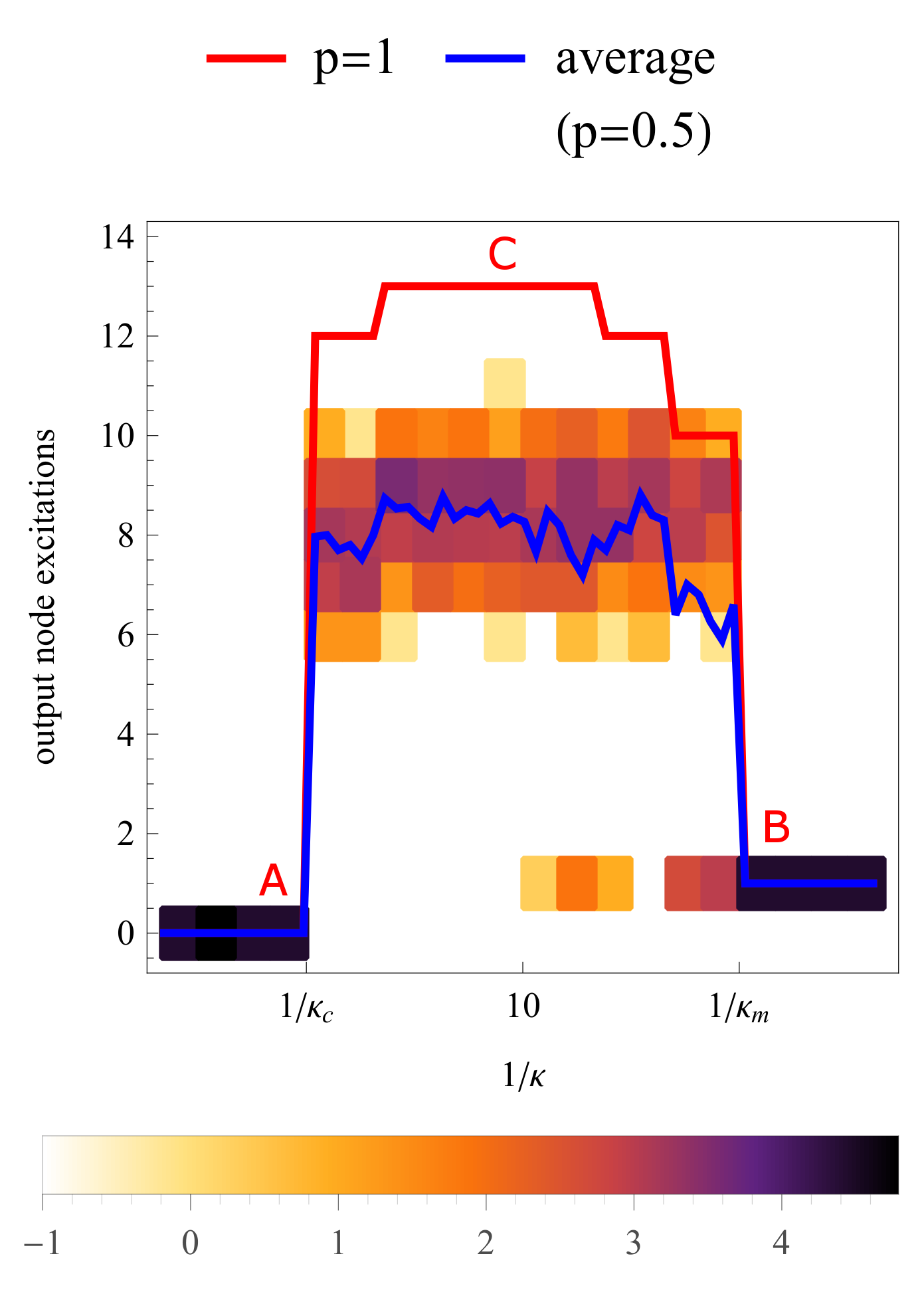
The difference between the behavior observed in case of a deterministic dynamics ($p=1$) and one where the random recovery ($p<1$) introduces an amount of stochasticity is enlightening. For $p<1$, one observes randomly distributed node failures as well as non zero output in the range $\kappa_{m}<\kappa<\kappa_{c}$ (region C). In fact the deterministic case delimits the possibility space of the stochastic case: All excitation levels that are possible for the deterministic dynamics are in principle achievable in the stochastic case, if the right nodes are susceptible again at the right moment. Inside of the ‘accessible region’ situations where a higher excitation level is achieved in the stochastic case, because a refractive node makes a ‘faster’ pacemaker accessible are conceivable. This exceptional event is rarely observed experimentally.

III.2 Prediction of response curve features

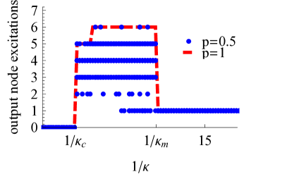
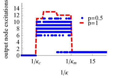
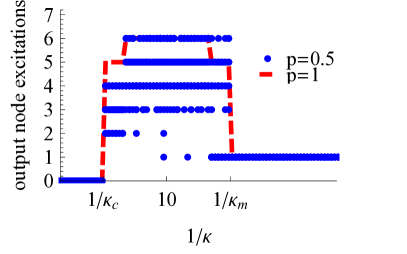
As pointed out in the previous Section, we can distinguish three parts or features in the curve at increasing $1/\kappa$, denoted A, B and C in the exemplary response curve shown in Figure 1 and in the additional examples in Figure 2. For each part of the curve, our qualitative explanation will be supported by the comparison of some quantitative prediction derived from network topological features with a large sample of simulation data (obtained with every possible input node for at least $50$ different networks of various average degree). Comparisons are visualized as scatter plots showing the (topologically) predicted transition value of $1/\kappa$ and the actually observed one in the simulated dynamics. Comparisons are then be made more quantitative by computing prediction quality (integrated over many networks) as a function of the relevant parameters, e.g. the average degree.

We denote $\kappa_{m}$ the value where the curve of accumulated excitations per output node markedly departs from 1 and has its first peak (point B), and $\kappa_{c}$ the value where the curve of accumulated excitations per output node goes to 0 (point A). Due to the definition of the relative threshold $\kappa$, the quantities $1/\kappa_{m}$ and $1/\kappa_{c}$ take only integer values when the average degree of the graph is varied (by varying the edge count $M$ at fixed number of nodes $N$).

III.2.1 Onset of excitation propagation (transition point A, $\kappa=\kappa_{c}$)

All curves display a critical threshold value $\kappa_{c}$ for the propagation of a single excitation from the input node to the output nodes. This threshold behavior in the absence of noise is analogous to an epidemic threshold. It does not depend on the value of $p$. For a finite network, the transition value $\kappa_{c}$ is a random variable depending on the realization of the network, the choice of the input node and of one among the possible output nodes, and of the initial configuration (here all nodes are initially susceptible).

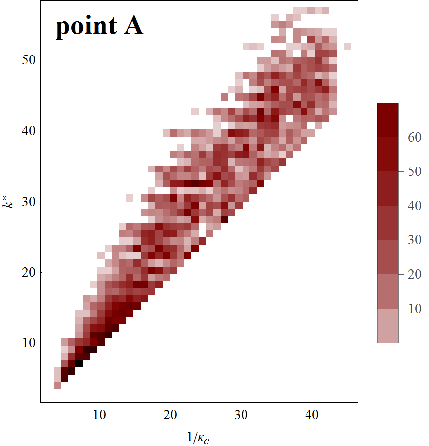
For $\kappa>\kappa_{c}$, before point A in Figure 1, $\kappa$ is so large that each possible path from the input node to an output node contains a barrier, that is, a node of large degree that cannot be excited by only one propagation excitation, and therefore no excitation reaches the output nodes. The network is then termed sub-threshold (as regards to $1/\kappa$, which can be roughly interpreted as a transmission probability). In other words, a sub-threshold situation could mean that on each linear path, there exists a node such that $k>1/\kappa$. Let $k^{*}$ be the largest degree encountered on the easiest paths to the output nodes, that is, the smallest over all paths to the output node of the maximal degree encountered along the path. Then the onset of excitation propagation is expected to arise for a value $1/\kappa_{c}=k^{*}$. This prediction is tested in Figure 3, where the topological observable $k^{*}$ is plotted as a function of the dynamic observable $1/\kappa_{c}$ for different networks. Another approach to predict $\kappa_{c}$ is to apply the same reasoning (largest degree encountered on the easiest path) but to not consider only the output node, but all nodes on the last layer. An improved prediction for $1/\kappa_{c}$ could thus be $k^{**}$, the minimum of the largest degrees encountered on the easiest path from the input node to any node in the output layer. However, the condition becomes less stringent, if the signal propagation activate redundant paths of the same length, so that more than one excitation may spontaneously arrive at a given node. We thus expect that $k^{*}$ and $k^{**}$ would give only an upper bound on $1/\kappa_{c}$, as supported by the asymmetry seen in Figure 3.

Looking at the system size dependence of our prediction quality, the most interesting phenomenon is the reduction of quality for larger BA graph due to many competing hubs (see Supplementary Material).

Figure 3: Density histogram of the predicted $k^{*}$ for the limit of sustained activity as a function of $1/\kappa_{c}$. The different values of $\kappa_{c}$ are obtained by running the dynamics on different network realizations and for different input nodes, while observing the topological observable $k^{*}$. Data are aggregated over graphs having $N=80$ nodes and $M=100...2000$ edges. The prediction is obtained by considering that the node with the highest degree on the easiest path (along which the maximal degree is minimal) from the input node to the output node is limiting.

Figure 4: A plot of the prediction quality for the limit $1/\kappa_{c}$ of sustained activity (transition point A). The data are obtained by scanning graphs having $N=80$ nodes and $M=100...2000$ edges. We shoe the predictions $k^{*}$ (solid red curve) and $k^{**}$ (dashed blue curve). Additionally the dashed green line indicates the expected failure of $k^{*}$ due to multiple excitations. Upper Figure: ER graphs; lower Figure: BA graphs.

The prediction quality is defined as the percentage of cases where $\kappa_{m}$ or $\kappa_{c}$ are predicted correctly. This is determined by comparing the topological prediction for $1/\kappa$ to the numerical result. The numerical result is obtained by a binary search in the space of $\kappa$. The inverse of this number is then rounded to the next integer, allowing an exact comparison. Note that, as we have observed that the transition value $\kappa_{m}$ does not depend on the value of $p$, we here use $p=1$ (the deterministic case) to make the binary search reliable.

A barrier may be passed in the case where two concurrent excitations reach it. The probability of such an event, that contributes to the discrepancy between our prediction and the observed value (and thus to the prediction quality), cannot be computed exactly. However, based on Eqs (1) - (3) (see Methods), we obtain a mean-field estimate of the importance of multiple excitations.

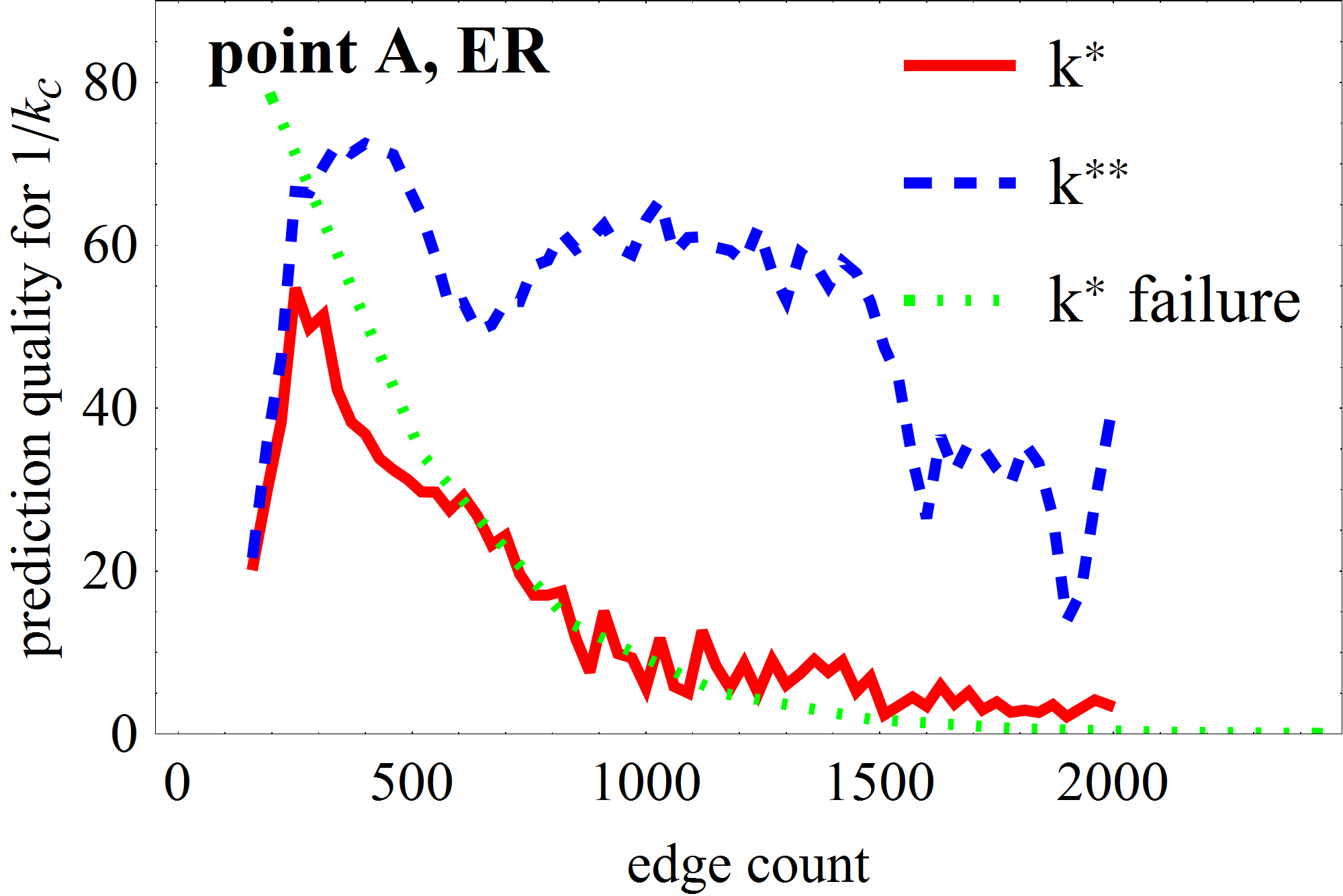
On this basis we can evaluate how multiple excitations contribute to the reduction observed in the quality of the prediction $1/\kappa_{c}=k^{*}$ with increasing link density in the graphs (see Figure 4).

The mean-field prediction of the effect of multiple excitations qualitatively explains the decrease of the prediction. As the mean-field approach is less reliable in the regime of very low excitation densities, we here use an intermediate value of $p$ ($p$=0.5) for the mean-field prediction. Even higher values show a similarly favorable comparison with the numerical simulation.

Note that this effect, the contribution from multiple excitations, does not explain the falsely predicted cases for sparse graphs. There, the difference to $100$ percent prediction quality must be due to the more complicated layer structure of sparse graphs. This observation is consistent with the fact that the discrepancy appears for the ER graph, but not for the BA graph, that has a more stable layer structure due to its hubs.

III.2.2 Transition between layer-wise propagation and sustained activity (transition point B, $\kappa=\kappa_{m}$)

By construction of the input-node-centered layer representation of the network, there are no shortcuts between non adjacent layers. At first, the excitation injected at the input node travels layer-wise, forming an excitation front reaching at each step a deeper layer. A jump arises in the output signal at some value $1/\kappa_{m}$ (transition point B). Typically a high-degree node, acting as a barrier, is not excited when the excitation front reaches its layer, and remains susceptible, leaving a susceptible ‘hole’ in a layer of refractory nodes. The amplification observed at point B, in $\kappa=\kappa_{m}$, and explained as the appearance of the first cycle, is sharp. This means that the cycle is traveled several times, or that other cycles can be excited after that the first one has stored excitation long enough for some refractory nodes to recover and provide substrate for further self-enhancing cycling excitation. Actually, the analysis of the simulated dynamics in its layered representation for several network realizations shows that as soon as a hole appears in the first layer, other holes rapidly appear in subsequent layers, thus supporting the possibility of cycling excitations, possibly numerous ones, and the sharp increase of the output signal. This mechanism to get re-entering excitation is quite similar to the mechanism for achieving curling in spiral wave formation Geberth:2008p525 ; Liao:2011be ; Garcia:2012ey : There must be a gap in the propagating front. Here either the excitation propagation meets a refractory node, or it fails to excite all the susceptible nodes that it encounters. It actually seems that any small perturbation of the sequential excitation of layers (observed in the low-$\kappa$ regime) is sufficient to trigger a full, self-sustained response with nearly saturated output nodes excitations.

Figure 5: A density histogram of the predicted degree for the onset of sustained activity (transition point B) as a function of $1/\kappa_{m}$. The data is aggregated over graphs having $N=80$ nodes and $M=100...2000$ edges. The prediction is that $1/\kappa_{m}=k_{max,1}(themaximaldegreeinthefirstlayer)$.

Figure 6: Prediction quality for the onset $1/\kappa_{m}$ of sustained activity. The data are obtained for graphs having $N=80$ nodes and $M=100...2000$ edges. The predictions are $1/\kappa_{m}=k_{max,1}$ (i.e., the maximal degree in the first layer, red solid curve) and $1/\kappa_{m}=k_{max}$ (i.e., the maximal degree, blue dashed curve). The upper panel is for ER graphs, while the lower panel is for BA graphs.

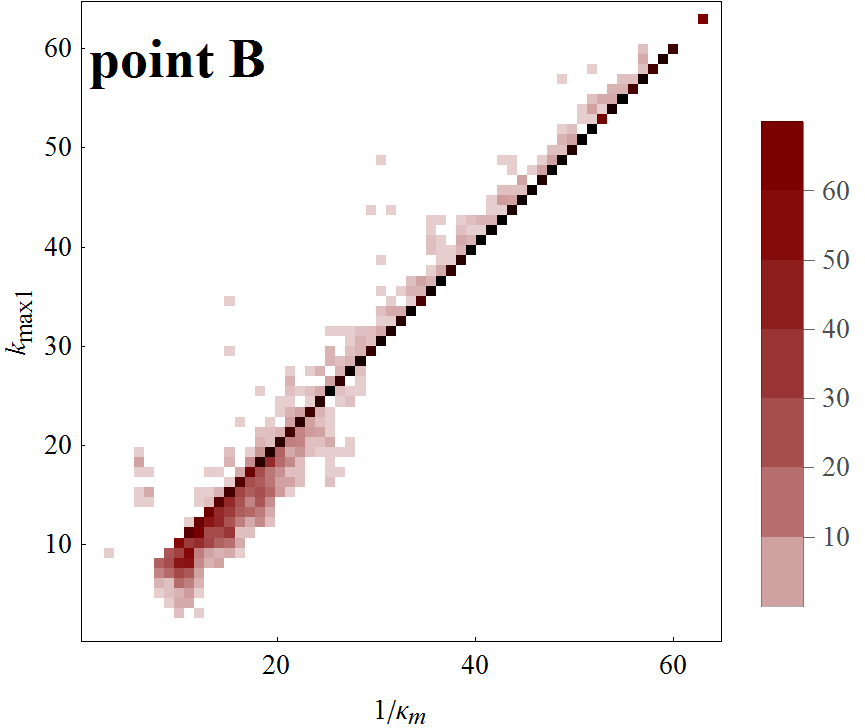
Denoting $k_{max}$ the maximal degree encountered in the network, a rough estimate of the jump location is $1/\kappa_{m}=k_{max}$. In fact, the degree distribution being layer-biased, it is expected that with a high probability the first hole appears in the first layer. Accordingly, another prediction is $1/\kappa_{m}=k_{max,1}$ where $k_{max,1}$ is the maximal degree encountered in the first layer.

The discrepancy with respect to our prediction of $\kappa_{m}$ is expected to mostly originate in situations where the first ‘hole’ (node remaining susceptible while the excitation front propagates downward the layers) is not located in the first layer. Additionally, an excitation hole does not necessarily trigger a cycle; it may also enable longer paths, arriving later at the output node (note that excitations do not accumulate: at a given moment, the excited output node contributes by 1 to the output signal, whatever the number of excited neighbors triggering it). For instance, the hole is excited a step later by concurring excitations coming from other nodes of the same layer, or two steps later by concurring excitations coming from other nodes of the next layer. This will also contribute to the discrepancy between our prediction and the actually observed value.

We compare our two predictions for $\kappa_{m}$, namely $1/k_{max}$ and $1/k_{max,1}$, for ER graphs (see Figure 5). Note that, as we have observed that the transition value $\kappa_{m}$ does not depend on the value of $p$, we here use $p=1$ (the deterministic case).

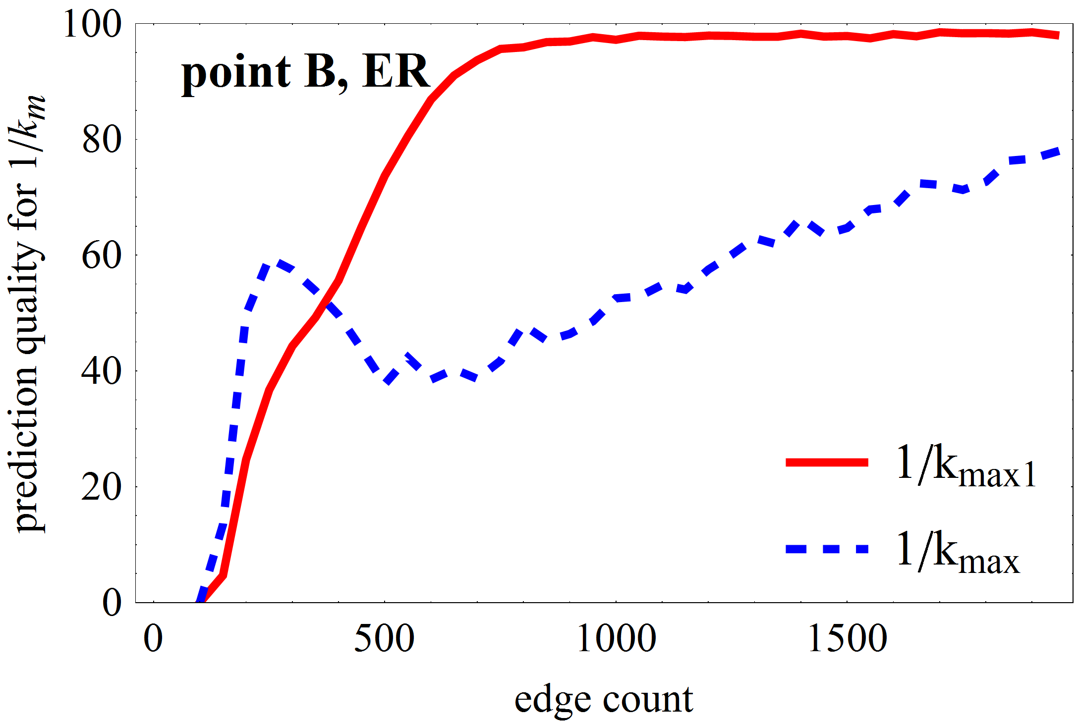
For dense networks (right part of the curves in Figure 6), the prediction $1/k_{max,1}$ has a 100% quality, meaning that a hole in the first layer is what conditions, directly or indirectly, the onset of a significant amplification. This effect can be more directly observed in Figure 5. As the network gets denser, the number of layers (the network maximal diameter) decreases, and the size of the first layer increases. We might think that soon, the node of maximal degree lies in the first layer. This is not the case, as shown by the discrepancy between the quality curves for the prediction $1/k_{max,1}$ and for the prediction $1/k_{max}$, which lies far below. If the node of maximal degree was in the first layer, then $k_{max,1}=k_{max}$ and the two curves would coincide. Hence, for dense graphs the presence of a hole in the first layer is important for signal propagation, while the hub of maximal degree is of no matter (although it would behave as a hole for smaller $\kappa$).

On the contrary, for sparse graphs, the prediction quality for $1/k_{max}$ outperforms the one based on $1/k_{max,1}$. When $\kappa$ is large enough for holes to appear in the first layer and be involved in recurrent excitation (cycles), the signal amplification is already working, due to a hole located in a deeper layer and having a degree $k_{max}>k_{max,1}$. What apparently matters most for signal amplification by recurrent (cycling) excitation is the delayed excitation of a global hub. What apparently matters in dense graphs is the delayed excitation of a hub in the first layer. At this point, it is difficult to say whether it is the presence of a hole per se which matters, or whether what matters are correlated features (e.g. the presence of a sufficient number of holes, or some more intricate feature of the available cycles). These higher-order conditions for the signal amplification setting in at this threshold value of $\kappa$ are the reason for the low prediction quality in the case of sparse graphs.

In fact, understanding these curves and improving our predictions ask for a better understanding of what happens after a ‘hole’ as appeared in the excitation front, and what are the requirements, in terms of either cycle statistics or paths statistics or presence of other holes (i.e. degeneracy of the degree $k_{max}$ or $k_{max,1}$), to get recurrent activity.

III.2.3 Height of the response curve (excitation level C)

The activity level at point C is linked to the appearance of cycling excitation, feeding (directly or indirectly) into the output node, up to the maximum where the output node is almost periodically excited, with the maximum average period $2+1/p$ for each value of the recovery probability $p$. In this region, the situation is presumably a set of redundant cycles, ensuring maximal excitation, so that on average an output node has one excitation every $2+1/p$ steps, yielding a (trivial) level of excitation equal to

$$\frac{T}{2+1/p}$$ (4)

where $T$ is the length of the recording.

We observe almost maximal excitation densities at the output nodes. This suggests that a set of redundant cycles compensates the stochasticity generated by the recovery probability $p$.

Figure 7 shows the maximal height of the response curve for various values of $p$ as a function of the edge density. As more and more cycles are formed by the added edges, the output node excitations quickly saturate at a value to a $p$-dependent level. The scaling of the output node saturation activity as a function of the refraction probability $p$ for dense graphs is shown in Figure 8.

The results are normalized so that its maximal capacity, for $p=1$, equals $100$, so that $a=300/(2+1/p)$. Generally, both the curves for the ER and the BA graph fit the prediction well. This prediction, merely equal to the output node capacity, constitutes an upper bound.

For Figure 7 we pick the maximum value of the output node excitation under variation of $\kappa$. In this way our numerical curve slightly overestimates the average maximum value predicted from Eq. (4).

The kink for small $p$ is due to an inability to sustain the activity due to small graph size combined with many refractory nodes. This finite size effect is further investigated in Figures 7 and 9, confirming that it disappears for larger graphs. This point emphasizes again the importance of studying small or medium-sized graphs, rather than just the asymptotic limit of infinite graphs, as real-world graphs across all domains of application (from biological to social and technological networks) tend to be comparatively small (with numbers of nodes mostly in the hundreds). In small networks, the topological details like the arrangement of cycles and the barrier structure are of importance for qualitative features of the dynamics, while for infinite graphs these details can be expected to average out.

When $p=1$, the dynamics is deterministic and sustained activity originating from robust pacemakers becomes possible, such as the triangle $ESR$ or the square $ESSR$ (see also Garcia:2012ey ). This setup yields an output excitation increasing linearly with the duration of the observation $T$. For $p<1$, the excitation ultimately vanishes in a finite network; however, for $p$ close enough to 1, a long transient activity is observed, during which the accumulated output signal increases with $T$. Practically the transient grows exponentially with $p$ and is longer than any reasonable simulation length, for example a network with $N=80$/$M=284$ reaches a transient length of $10^{6}$ around $p=0.4$.

Figure 7: The maximum height of the output signal for different values of $p$. The bottom level (output node) activity is normalized such that $100$ corresponds to the maximal capacity of the output node at $p=1$. The number of edges $M$ is varied, while the number of nodes is constant ($N$ = 80). For dense graphs, the sustained activity saturates to a value dependent on $p$. The number of output excitations is aggregated over $T=600$ steps, so that shorter transients do not matter.

Figure 8: The scaling of the bottom level (output node) saturation activity over the recovery probability $p$ for dense ER and BA graphs ($N=80$,$M=640$). The output node activity $a$ is normalized such that $100$ corresponds to its maximal capacity, at $p=1$. The ER graphs (solid red curve) and the BA graphs (dashed blue curve) behave very similarly. Additionally a prediction curve is included ($a=300/(2+1/p)$) in dashed green.

Figure 9: The scaling of the bottom level (output node) saturation activity over the refraction probability $p$ for dense ER graphs of different sizes. The output node activity $a$ is normalized such that $100$ corresponds to its maximal capacity at $p=1$. Additionally a prediction curve is included ($a=300/(2+1/p)$) as a thin black line.

IV Discussion and Conclusion

The observed phenomena can be classified as ‘path-driven’ (for the transition in A, $\kappa=\kappa_{c}$) and ‘cycle-driven’ (for the transition in B, $\kappa=\kappa_{m}$). Indeed, the transition between sub-threshold (no propagation to the output nodes) and supra-threshold dynamics is due to the appearance of the first barrier-free path. On the contrary, the transition between simple signal propagation and signal amplification is due to topological cycles and the possibility of cycling excitation that occurs as soon as some nodes are not excited in the first stage of signal propagation. Cycling excitation is involved at low $\kappa$, explaining the amplification of the output signal once a hole as appeared in the excitation front (currently in the first layer).

The layer representation starting from a given node provides a node-centered view that a given individual node may have of the network in which it is embedded. This view is relevant in several instances, such as the local probing of a network with no possibility to have an overall and external view, e.g. probing the internet, propagation of signals in neural networks, social networks in which an individual has only a subjective view of the network to which s/he belongs, local control of a logistic or engineered network in which only some localized nodes can be acted upon. At intermediary values of $\kappa$, the excitation dynamics is sensitive to the hierarchical layer representation of the network. In this sense, we have a process-induced layering, which could also happen in real networks, of a few input nodes have been specifically selected and evolved to match suitable topological features for the relevant dynamics.

Our simple numerical experiment and its interpretation provide a reference case illustrating typical topological mechanisms that can be at work in shaping the propagation and amplification of a signal in an excitable network. Among the mechanisms we specially underline propagation due to a huge path redundancy and amplification due to cycling excitations. Our study enlightens the topological preconditions of spontaneous activity, which is of relevance to understand which topological properties of a neural network enhance resting state activity Deco:2009p6486 ; Deco:2011p775 . Moreover, these properties also form the precondition for the specific reverberations that may serve as a dynamic representation of memory. When $p<1$, cycle multiplicity seems essential to sustained activity, because each individual cycle will have a very limited activity. The values of $\kappa_{m}$ and $\kappa_{c}$ provide a way to calibrate different graphs when investigating for instance the influence of the architecture on the dynamic behavior. The difference $\kappa_{c}$-$\kappa_{m}$ can be taken as a unit for $\kappa$.

A vast amount of studies attempted to understand how network topology affects simple dynamical processes. Examples of such processes include synchronization Arenas:2006ba ; deArruda:2013hd , random walks Menezes2004FluctuationsinNetwork and the propagation of excitations through networks MullerLinow:2006ex ; Garcia:2012ey .

We explored how network topology determines the probability of dynamical events regulating the onset of persistent excitable dynamics (transition point A, Figure 3) in a graph, as well as the transition from propagating waves to sustained activity (transition point B, Figure 5) as a function of the relative excitation threshold. We use single excitations to probe the networks’ dynamical capabilities as a minimal numerical experiment to gain insight into the mechanism underlying these two transitions. Our investigation thus sheds light on a situation of high interest to statistical physics: How do network details determine the propagation of excitations through a given network. We find that the excitation threshold selects certain topological constellations in the network, which serve as dynamical seeds initiating these transitions.

Here, each graph has its own individual thresholds for the two transitions. Our mechanistic understanding of the dynamics is sufficient for predicting these two thresholds on the basis of topological information alone. This statement is validated by evaluating the prediction quality across a wide range of graphs.

Two result have been described in this paper: (1) For a specific graph, we can predict the critical threshold values. In spite of the similarities on the qualitative level, the response curves can look very different in the details (transition points, height) depending on the specific choice of the input node. This is due to the fact that, seen from one input node, a highly specific barrier structure on the paths towards the output node is encountered, as well as a specific arrangement of cycles along these paths. As we have demonstrated with the numerical experiments described in this paper, these topological details directly affect the response curve. (2) Our investigation draws the attention to a new network property: the barrier and cycle structures of networks, when hierarchized from specific input nodes. In evolved networks (like cortical area networks) this observation suggests the possibility of identifying input and output nodes via an optimized (or evolutionarily shaped) barrier and cycle structure along the interlinking paths.

In order to make the study more relevant for understanding sustained activity is real-world and particularly neural networks, it would naturally be very interesting to expand the focus to (i) structured, non-random networks (e.g., what would be effect of ring lattice Vishwanathan:2011it , modular or hierarchical architectures), (ii) consider the different dynamic patterns induced by specific stimulation of different input nodes. In particular understand, to what extent do such specific stimulations lead to reproducible patterns of activity.

However, our set of results can already be used in real cases or more complicated numerical situations as a basis for delineating the contribution due to these simple mechanisms and the contribution due to the involvement of additional and more specific mechanisms. Unraveling the coupled dynamical and topological origin of the different features of the curve clearly shows the articulation between a regime dominated by cycling excitation and a regime controlled by barriers along linear (possibly redundant, as in an oriented mesh) paths.

References

- (1) Arenas, A., Díaz-Guilera, A., Pérez-Vicente, C.: Synchronization reveals topological scales in complex networks. Physical Review Letters 96(11), 114102 (2006)
- (2) de Arruda, G.F., Dal’Maso Peron, T.K., de Andrade, M.G., Achcar, J.A., Rodrigues, F.A.: The influence of network properties on the synchronization of kuramoto oscillators quantified by a bayesian regression analysis. Journal of Statistical Physics 152(3), 519–533 (2013)
- (3) Azouz, R., Gray, C.M.: Dynamic spike threshold reveals a mechanism for synaptic coincidence detection in cortical neurons in vivo. Proceedings of the National Academy of Sciences of the United States of America 97(14), 8110–8115 (2000)
- (4) Barabasi, A., Albert, R.: Emergence of scaling in random networks. Science 286(5439), 509 (1999)
- (5) Benda, J., Herz, A.V.: A universal model for spike-frequency adaptation. Neural Computation 15(11), 2523–2564 (2003)
- (6) Bornholdt, S.: Systems biology: less is more in modeling large genetic networks. Science Signaling 310(5747), 449 (2005)
- (7) Deco, G., Jirsa, V., McIntosh, A., Sporns, O., Kötter, R.: Key role of coupling, delay, and noise in resting brain fluctuations. Proceedings of the National Academy of Sciences of the United States of America (2009)
- (8) Deco, G., Jirsa, V.K., Mcintosh, A.R.: Emerging concepts for the dynamical organization of resting-state activity in the brain. Nat. Rev. Neurosci. 12(1), 43–56 (2011)
- (9) Garcia, G., Lesne, A., Hilgetag, C., Hütt, M.: Role of long cycles in excitable dynamics on graphs. Phys. Rev. E 90(5), 052805 (2014)
- (10) Garcia, G.C., Lesne, A., Hütt, M., Hilgetag, C.C.: Building blocks of self-sustained activity in a simple deterministic model of excitable neural networks. Frontiers in computational neuroscience 6, 50 (2012)
- (11) Geberth, D., Hütt, M.T.: Predicting spiral wave patterns from cell properties in a model of biological self-organization. Phys. Rev. E 78(3), 1–9 (2008)
- (12) Giaquinta, A., Argentina, M., Velarde, M.G.: A simple generalized excitability model mimicking salient features of neuron dynamics. Journal of Statistical Physics 101(1-2), 665–678 (2000)
- (13) Graham, I., Matthai, C.C.: Investigation of the forest-fire model on a small-world network. Physical Review E 68(3), 036109 (2003)
- (14) Hadipour Niktarash, A.: Discussion on the reverberatory model of short-term memory: A computational approach. Brain and Cognition 53(1), 1–8 (2003)
- (15) Hebb, D.O.: The organization of behavior. Wiley, New York (1949)
- (16) Hütt, M.T., Hilgetag, C.C., Kaiser, M.: Network-guided pattern formation of neural dynamics. Philosophical Transactions of the Royal Society of London. Series B, Biological Sciences 369(1653), 20130522 (2014)
- (17) Hütt, M.T., Jain, M.K., Hilgetag, C.C., Lesne, A.: Stochastic resonance in discrete excitable dynamics on graphs. Chaos, Solitons & Fractals 45(5), 611–618 (2012)
- (18) Hütt, M.T., Lesne, A.: Interplay between topology and dynamics in excitation patterns on hierarchical graphs. Frontiers in neuroinformatics 3, 28 (2009)
- (19) Lewis, T., Rinzel, J.: Self-organized synchronous oscillations in a network of excitable cells coupled by gap junctions. Network: Comput. Neural Syst. 11(4), 299–320 (2000)
- (20) Li, W.: Phenomenology of nonlocal cellular automata. Journal of Statistical Physics 68(5-6), 829–882 (1992)
- (21) Liao, X., Xia, Q., Qian, Y., Zhang, L., Hu, G., Mi, Y.: Pattern formation in oscillatory complex networks consisting of excitable nodes. Physical Review E 83(5), 056204 (2011)
- (22) Liao, X.H., Qian, Y., Mi, Y., Xia, Q.Z., Q., H.X., Hu, G.: Oscillation sources and wave propagation paths in complex networks consisting of excitable nodes. Frontiers of Physics 6, 124–132 (2011)
- (23) Marr, C., Hütt, M.T.: Outer-totalistic cellular automata on graphs. Physics Letters A 373(5), 546–549 (2009)
- (24) Marr, C., Hütt, M.T.: Cellular automata on graphs: Topological properties of er graphs evolved towards low-entropy dynamics. Entropy 14(6), 993–1010 (2012)
- (25) McGraw, P., Menzinger, M.: Self-sustaining oscillations in complex networks of excitable elements. Physical Review E 83(3), 037102 (2011)
- (26) de Menezes, M.A., Barabási, A.L.: Fluctuations in network dynamics. Phys. Rev. Lett. 92(2), 028701 (2004)
- (27) Messé, A., Hütt, M., König, P., Hilgetag, C.: A closer look at the apparent correlation of structural and functional connectivity in excitable neural networks. Scientific Reports submitted (2014)
- (28) Moreno, Y., Pastor-Satorras, R., Vespignani, A.: Epidemic outbreaks in complex heterogeneous networks. The European Physical Journal B 26(4), 521 (2002)
- (29) Müller-Linow, M., Hilgetag, C.C., Hütt, M.T.: Organization of Excitable Dynamics in Hierarchical Biological Networks. PLoS Computational Biology 4(9), e1000190 (2008)
- (30) Müller-Linow, M., Marr, C., Hütt, M.: Topology regulates the distribution pattern of excitations in excitable dynamics on graphs. Physical Review E 74(1), 1–7 (2006)
- (31) Muresan, R.C., Savin, C.: Resonance or integration? Self-sustained dynamics and excitability of neural microcircuits. Journal of Neurophysiology 97(3), 1911–1930 (2007)
- (32) Pastor-Satorras, R., Vespignani, A.: Epidemic spreading in scale-free networks. Physical Review Letters 86(14), 3200 (2001)
- (33) Qian, Y., Huang, X., Hu, G., Liao, X.: Structure and control of self-sustained target waves in excitable small-world networks. Physical Review E 81, 036101 (2010)
- (34) Qian, Y., Liao, X., Huang, X., Mi, Y., Zhang, L., Hu, G.: Diverse self-sustained oscillatory patterns and their mechanisms in excitable small-world networks. Physical Review E 82(2), 026107 (2010)
- (35) Roxin, A., Riecke, H., Solla, A.: Self-sustained activity in a small-world network of excitable neurons. Physical Review Letters 92(19), 198,101 (2004)
- (36) Tegnér, J., Compte, A., Wang, X.J.: The dynamical stability of reverberatory neural circuits. Biological Cybernetics 87(5-6), 471–481 (2002)
- (37) Vishwanathan, A., Bi, G.Q., Zeringue, H.C.: Ring-shaped neuronal networks: a platform to study persistent activity. Lab on a chip 11(6), 1081–1088 (2011)
- (38) Vladimirov, N., Tu, Y., Traub, R.D.: Shortest loops are pacemakers in random networks of electrically coupled axons. Frontiers in Computational Neuroscience 6, 17 (2012)
- (39) Wang, X.J.: Synaptic reverberation underlying mnemonic persistent activity. Trends in Neurosciences 24(8), 455–463 (2001)