First-order weak balanced schemes for bilinear stochastic differential equations

Abstract

We use the linear scalar SDE as a test problem to show that it is possible to construct almost sure stable first-order weak balanced schemes based on the addition of stabilizing functions to the drift terms. Then, we design balanced schemes for multidimensional bilinear SDEs achieving the first order of weak convergence, which do not involve multiple stochastic integrals. To this end, we follow two methodologies to find appropriate stabilizing weights; through an optimization procedure or based on a closed heuristic formula. Numerical experiments show a promising performance of the new numerical schemes.

1 Introduction

Consider the autonomous stochastic differential equation (SDE)

$$X_{t}=X_{0}+\int_{0}^{t}b\left(X_{s}\right)ds+\sum_{k=1}^{m}\int_{0}^{t}\sigma^{k}\left(X_{s}\right)dW^{k}_{s},$$ (1)

where $\left(X_{t}\right)_{t\geq 0}$ is an adapted $\mathbb{R}^{d}$-valued stochastic process, $b,\sigma^{k}:\mathbb{R}^{d}\rightarrow\mathbb{R}^{d}$ are smooth functions and $W^{1},\ldots,W^{m}$ are independent standard Wiener processes. For solving (1) in cases the diffusion terms $\sigma^{k}$ play an essential role in the dynamics of $X_{t}$, Milstein, Platen and Schurz [1] introduced the balanced method

$$\begin{split}Z_{n+1}&=Z_{n}+b\left(Z_{n}\right)\Delta+\sum_{k=1}^{m}\sigma^{k}\left(Z_{n}\right)\left(W^{k}_{\left(n+1\right)\Delta}-W^{k}_{n\Delta}\right)\\ &\quad+\left(c^{0}\left(Z_{n}\right)\Delta+\sum_{k=1}^{m}c^{k}\left(Z_{n}\right)\left|W^{k}_{\left(n+1\right)\Delta}-W^{k}_{n\Delta}\right|\right)\left(Z_{n}-Z_{n+1}\right),\end{split}$$ (2)

where $\Delta>0$ and $c^{0},c^{1},\ldots,c^{m}$ are weight functions that should be appropriately chosen for each SDE. Up to now, the schemes of type (2) use the damping functions $c^{1},\ldots,c^{m}$ to avoid the numerical instabilities caused by $\sigma^{k}$ or to have $a.s.$ positivity (see, e.g., [1, 2, 3, 4, 5]), and hence their rate of weak convergence is equal to $1/2$, which is low. To the best of our knowledge, concrete balanced versions of the Milstein scheme have been developed only in particular cases, like $m=1$, where the Milstein scheme does not involve multiple stochastic integrals with respect to different Brownian motions [6, 7].

We are interested in the development of efficient first weak order schemes for computing $\mathbb{E}f\left(X_{t}\right)$, with $f:\mathbb{R}^{d}\rightarrow\mathbb{R}$ smooth. This motivates the design of balanced schemes based only on $c_{0}$, whose rate of weak convergence is equal to $1$ under general conditions (see, e.g., [3, 4]). In this direction, [3, 4] propose to take $c^{0}=0.5\,\nabla b$, together with $c^{1}=\cdots=c^{m}=0$. This choice contains no information about the diffusion terms $\sigma^{k}$, and yields unstable schemes in situations like $dX_{t}=\lambda X_{t}\,dW^{1}_{t},$ with $\lambda>0$ and $X_{t}\in\mathbb{R}$; a test equation used to introduce the balanced schemes (see [1]).

This paper addresses the question of whether we can find $c^{0}$ such that

$$Z_{n+1}=Z_{n}+b\left(Z_{n}\right)\Delta+c^{0}\left(\Delta,Z_{n}\right)\left(Z_{n+1}-Z_{n}\right)\Delta+\sum_{k=1}^{m}\sigma^{k}\left(Z_{n}\right)\sqrt{\Delta}\xi_{n}^{k}$$ (3)

reproduces the long-time behavior of $X_{t}$, where from now on $\xi_{0}^{1},\xi_{0}^{2},\ldots,\xi_{0}^{m},\xi_{1}^{1},\ldots$ are independent random variables satisfying $\mathbf{P}\left(\xi_{n}^{k}=\pm 1\right)=1/2$. Section 2 gives a positive answer to this problem when (1) reduces to the classical scalar SDE

$$X_{t}=X_{0}+\int_{0}^{t}\mu X_{s}ds+\int_{0}^{t}\lambda X_{s}dW^{1}_{s}$$ (4)

where $\mu,\lambda\in\mathbb{R}$. Indeed, we obtain an explicit expression for $c^{0}\left(\Delta,\cdot\right)$ that makes $Z_{n}$ almost sure asymptotically stable for all $\Delta>0$ whenever $2\mu-\lambda^{2}<0$, as well as positive preserving. In Section 3, we propose an optimization procedure for identifying a suitable weight function $c_{0}$ in case $b,\sigma^{k}:\mathbb{R}^{d}\rightarrow\mathbb{R}^{d}$ are linear, and we also provides a choice of $c_{0}$ based on a heuristic closed formula. Both techniques show good results in our numerical experiments, which encourages further studies of (3). All proofs are deferred to Section 4.

2 Stabilized Euler scheme for the linear scalar SDE

In this section $X_{t}$ satisfies (4), which is a classical test equation for studying the stability properties of the numerical schemes for (1) (see, e.g., [2, 8, 9]). We assume, for simplicity, that $2\mu-\lambda^{2}<0$. Set $T_{n}=n\Delta$, where $\Delta>0$ and $n=0,1,\ldots$ For all $t\in\left[T_{n},T_{n+1}\right]$ we have

$$X_{t}=X_{T_{n}}+\int_{T_{n}}^{t}\left(\mu X_{s}+a\left(\Delta\right)X_{s}-a\left(\Delta\right)X_{s}\right)ds+\int_{T_{n}}^{t}\lambda X_{s}dW^{1}_{s},$$

where $a\left(\Delta\right)$ is an arbitrary real number. Then

$$X_{T_{n+1}}\approx X_{T_{n}}+\mu X_{T_{n}}\Delta+a\left(\Delta\right)\left(X_{T_{n+1}}-X_{T_{n}}\right)\Delta+\lambda X_{T_{n}}\left(W^{1}_{T_{n+1}}-W^{1}_{T_{n}}\right),$$

and so $X_{t}$ is weakly approximated by the recursive scheme

$$Y^{s}_{n+1}=Y^{s}_{n}+\mu Y^{s}_{n}\Delta+a\left(\Delta\right)\left(Y^{s}_{n+1}-Y^{s}_{n}\right)\Delta+\lambda Y^{s}_{n}\sqrt{\Delta}\xi^{1}_{n}.$$ (5)

In case $a\left(\Delta\right)\Delta\neq 1$, we have

$$Y^{s}_{n+1}=Y^{s}_{n}\left(1+\left(\mu\Delta+\lambda\sqrt{\Delta}\xi^{1}_{n}\right)/\left(1-a\left(\Delta\right)\Delta\right)\right).$$

We wish to find a locally bounded function $\Delta\mapsto a\left(\Delta\right)$ such that:

P1)

$Y^{s}_{n}$ preserves $a.s.$ the sign of $Y^{s}_{0}$ for all $n\in\mathbb{N}$.

P2)

$Y^{s}_{n}$ converges almost surely to $0$ as $n\rightarrow\infty$ whenever $2\mu-\lambda^{2}<0$.

We check easily that Property P1 holds iff $a\left(\Delta\right)\in\left]-\infty,p_{1}\right[\cup\left]p_{2},+\infty\right[,$ with $p_{1}:=\min\left\{1,1-\left|\lambda\right|\sqrt{\Delta}+\mu\Delta\right\}/\Delta$ and $p_{2}:=\max\left\{1,1+\left|\lambda\right|\sqrt{\Delta}+\mu\Delta\right\}/\Delta$. A close look at $\mathbb{E}\log\left(1+\left(\mu\Delta+\lambda\sqrt{\Delta}\xi^{1}_{n}\right)/\left(1-a\left(\Delta\right)\Delta\right)\right)$ reveals that:

Lemma 1.

Suppose that $a\left(\Delta\right)\Delta\neq 1$. Then, a necessary and sufficient condition for Property P1, together with $\lim_{n\rightarrow\infty}Y^{s}_{n}=0$ $a.s.$, is that

$$\begin{cases}a\left(\Delta\right)\in\left]-\infty,p_{1}\right[\cup\left]p_{2},p_{3}\right[,&\text{in case }\mu<0\\ a\left(\Delta\right)\in\left]-\infty,p_{1}\right[\cup\left]p_{2},+\infty\right[,&\text{in case }\mu=0\text{ and }\lambda\neq 0\par\\ a\left(\Delta\right)\in\left]p_{3},p_{1}\right[\cup\left]p_{2},+\infty\right[,&\text{in case }\mu>0\end{cases}$$

where $p_{3}:=\left(\mu^{2}\Delta+2\mu-\lambda^{2}\right)/\left(2\mu\Delta\right)$.

Using Lemma 1 we deduce that we can choose

$$a\left(\Delta\right)=\begin{cases}\mu-\alpha_{1}\left(\Delta\right)\lambda^{2},&\text{if }\mu\leq 0\\ \mu-\alpha_{2}\left(\Delta\right)\lambda^{2},&\text{if }\mu>0\text{ and }\Delta<2/\mu\\ \left(1+\left|\lambda\right|\sqrt{\Delta}+\mu\Delta\right)/\Delta+\beta,&\text{if }\mu>0\text{ and }\Delta\geq 2/\mu\end{cases}$$ (6)

where $\beta>0$, $1/4<\alpha_{2}\left(\Delta\right)\leq 1/4+\left(\lambda^{2}-2\mu\right)\left(2-\mu\Delta\right)/\left(8\lambda^{2}\right)$ and $\alpha_{1}$ is a bounded function satisfying $\alpha_{1}\left(\Delta\right)>1/4$.

Theorem 2.

Let $2\mu-\lambda^{2}<0$. Then, $Y^{s}_{n}$ with $a\left(\Delta\right)$ given by (6) satisfies Properties P1 and P2.

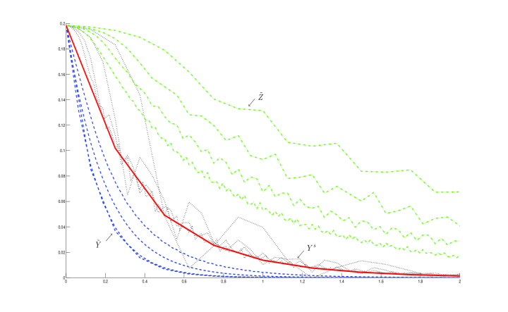
Figure 1: Computation of $\mathbb{E}\sin\left(X_{t}/5\right)$, where $t\in\left[0,2\right]$ and $X_{t}$ solves (4) with $\mu=0$, $\lambda=4$ and $X_{0}=1$. Dashed line: $\tilde{Y}$, dashdot line: $\tilde{Z}$, dotted line: $Y^{s}$, and solid line: reference values. Here, $\Delta$ takes the values $1/8$, $1/16$, $1/32$ and $1/64$. As we expected, smaller $\Delta$ produce better approximations.

Following [1], we now illustrate the behavior of $Y^{s}_{n}$ using (4) with $\mu=0$ and $\lambda=4$. We take $X_{0}=1$. Since $\mu\leq 0$, we choose $\alpha_{1}\left(\Delta\right)=1/4+1/100$; its convenient to keep the weights as small as possible. Figure 1 displays the computation of $\mathbb{E}\sin\left(X_{t}/5\right)$ obtained from the sample means of $25\cdot 10^{9}$ observations of: $Y^{s}_{n}$ with $a\left(\Delta\right)=-0.26\ \lambda^{2}$, the fully implicit method $\tilde{Y}_{n+1}=\tilde{Y}_{n}/\left(1+\lambda^{2}\Delta-\lambda\sqrt{\Delta}\xi^{1}_{n}\right)$ (see p. 497 of [10]), and the balanced scheme

$$\widetilde{Z}_{n+1}=\widetilde{Z}_{n}\left(1+\lambda\sqrt{\Delta}\xi^{1}_{n}+\lambda\sqrt{\Delta}\right)/\left(1+\lambda\sqrt{\Delta}\right),$$

which is a weak version of the method developed in Section 2 of [1]. $\widetilde{Z}_{n}$ preserves the sign of $\widetilde{Z}_{0}$ and is almost sure asymptotically stable (see [4]). Solid line identifies the ‘true’ values gotten by sampling $25\cdot 10^{9}$ times $\exp\left(-8t+4W_{t}\right)$.

In contrast with the poor performance of the Euler-Maruyama scheme when the step sizes are greater than or equal to $1/16$, Figure 1 suggests us that $Y^{s}_{n}$ is an efficient scheme having good qualitative and convergence properties. In this numerical experiment, the accuracy of $\tilde{Z}_{n}$ is not good, and $\tilde{Y}_{n}$ decays too fast to $0$ as $n\rightarrow\infty$.

3 System of bilinear SDEs

This section is devoted to the SDE

$$X_{t}=X_{0}+\int_{0}^{t}BX_{s}ds+\sum_{k=1}^{m}\int_{0}^{t}\sigma^{k}X_{s}dW_{s}^{k},$$ (7)

where $X_{t}\in\mathbb{R}^{d}$ and $B,\sigma^{k}\in\mathbb{R}^{d\times d}$. The bilinear SDEs describe dynamical features of non-linear SDEs via the linearization around their equilibrium points (see, e.g., [11]). The system of SDEs (7) also appears, for example, in the spatial discretization of stochastic partial differential equations (see, e.g., [12, 13]).

3.1 Heuristic balanced scheme

Since (7) is bilinear, we restrict $c^{0}$ to be constant, and so (3) becomes

$$Z_{n+1}=Z_{n}+BZ_{n}\Delta+H\left(\Delta\right)\left(Z_{n+1}-Z_{n}\right)\Delta+\sum_{k=1}^{m}\sigma^{k}Z_{n}\sqrt{\Delta}\xi^{k}_{n},$$ (8)

with $H:\left]0,\infty\right[\rightarrow\mathbb{R}^{d\times d}$ and $\Delta>0$. The rate of weak convergence of $Z_{n}$ is equal to $1$ provided, for instance, that $H\left(\Delta\right)$ and $\left(I-\Delta H\left(\Delta\right)\right)^{-1}$ are bounded on any interval $\Delta\in\left]0,a\right]$ (see, e.g., [3]). Generalizing roughly Section 2 we choose $H\left(\Delta\right)=B-\sum\limits_{k=1}^{m}\alpha_{k}\left(\Delta\right)\left(\sigma^{k}\right)^{\top}\sigma^{k},$ where, for example, $\alpha_{k}\left(\Delta\right)=0.26$. This gives the recursive scheme

$$\begin{split}\left(I-\Delta B+0.26\ \Delta\sum\limits_{k=1}^{m}\left(\sigma^{k}\right)^{\top}\sigma^{k}\right)Y^{s}_{n+1}&=Y^{s}_{n}+0.26\ \Delta\sum\limits_{k=1}^{m}\left(\sigma^{k}\right)^{\top}\sigma^{k}Y^{s}_{n}\\ &\quad+\sum_{k=1}^{m}\sigma^{k}Y^{s}_{n}\sqrt{\Delta}\xi^{k}_{n},\end{split}$$ (9)

which is a first-order weak balanced version of the semi-implicit Euler method.

Remark 1.

Combining (9) with ideas of the local linearization method (see, e.g., [14, 15]) we deduce the following numerical method for (1):

$$U_{n+1}=U_{n}+b\left(U_{n}\right)\Delta+\sum_{k=1}^{m}\sigma^{k}\left(U_{n}\right)\sqrt{\Delta}\xi^{k}_{n}+H\left(\Delta,U_{n}\right)\left(U_{n+1}-U_{n}\right)\Delta,$$

where $H\left(\Delta,x\right)=\nabla b\left(x\right)-\sum\limits_{k=1}^{m}\alpha_{k}\left(\Delta\right)\left(\nabla\sigma^{k}\left(x\right)\right)^{\top}\nabla\sigma^{k}\left(x\right)$ with $\alpha_{k}\left(\Delta\right)=0.26$.

3.2 Optimal criterion to select $c_{0}$

In case $I-\Delta H\left(\Delta\right)$ is invertible, according to (8) we have

$$Z_{n+1}=Z_{n}+\left(I-\Delta H\left(\Delta\right)\right)^{-1}\left(\Delta B+\sum_{k=1}^{m}\sqrt{\Delta}\xi^{k}_{n}\sigma^{k}\right)Z_{n},$$ (10)

where $I$ is the identity matrix. Therefore, a more general formulation of $Z_{n}$ is

$$V_{n+1}=V_{n}+\left(I+\Delta M\left(\Delta\right)\right)\left(\Delta B+\sum_{k=1}^{m}\sqrt{\Delta}\xi^{k}_{n}\sigma^{k}\right)V_{n},$$ (11)

with $M:\left]0,\infty\right[\rightarrow\mathbb{R}^{d\times d}$. In fact, taking $M\left(\Delta\right)=\left(\left(I-\Delta H\left(\Delta\right)\right)^{-1}-I\right)/\Delta$ we obtain (10) from (11). The following theorem provides a useful estimate of the growth rate of $V_{n}$ in terms of $\mathbb{E}\log\left(\left\|A_{0}\left(\Delta,M\left(\Delta\right)\right)x\right\|\right)$, a quantity that we can compute explicitly in each specific situation.

Theorem 3.

Let $V_{n}$ be defined recursively by (11). Then

$$\lim_{n\rightarrow\infty}\frac{1}{n\Delta}\log\left(\left\|V_{n}\right\|\right)\leq\frac{1}{\Delta}\sup_{x\in\mathbb{R}^{d},\left\|x\right\|=1}\mathbb{E}\log\left(\left\|A_{n}\left(\Delta,M\left(\Delta\right)\right)x\right\|\right),$$ (12)

where $A_{n}\left(\Delta,M\right)=I+\left(I+\Delta M\right)\left(\Delta B+\sum_{k=1}^{m}\sqrt{\Delta}\xi^{k}_{n}\sigma^{k}\right)$.

Set $\ell:=\sup_{x\in\mathbb{R}^{d},\left\|x\right\|=1}\left(\langle x,Bx\rangle+\frac{1}{2}\sum_{k=1}^{m}\left\|\sigma^{k}x\right\|^{2}-\sum_{k=1}^{m}\langle x,\sigma^{k}x\rangle^{2}\right)$. Then

$$\limsup_{t\rightarrow\infty}\frac{1}{t}\log\left(\left\|X_{t}\right\|\right)\leq\ell\hskip 28.45274pta.s.$$ (13)

(see, e.g., [9]). Fix $\Delta>0$. We would like that for all $\left\|x\right\|=1$,

$$\frac{1}{\Delta}\mathbb{E}\log\left(\left\|A_{0}\left(\Delta,M\left(\Delta\right)\right)x\right\|\right)\approx\langle x,Bx\rangle+\frac{1}{2}\sum_{k=1}^{m}\left\|\sigma^{k}x\right\|^{2}-\sum_{k=1}^{m}\langle x,\sigma^{k}x\rangle^{2}.$$

A simpler problem is to find $M\left(\Delta\right)$ for which the upper bounds (12) and (13) are as close as possible, and so we can expect that $V_{n}$ inherits the long-time behavior of $X_{t}$. Then, we propose to take

$$M\left(\Delta\right)\in\operatornamewithlimits{arg\ min}\left\{\left(\frac{1}{\Delta}\sup_{x\in\mathbb{R}^{d},\left\|x\right\|=1}\mathbb{E}\log\left(\left\|A_{0}\left(\Delta,M\right)x\right\|\right)-\ell\right)^{2}:M\in\mathcal{M}\right\},$$ (14)

where $\mathcal{M}$ is a predefined subset $\mathbb{R}^{d\times d}$. Two examples of $\mathcal{M}$ used successfully in our numerical experiments are $\mathbb{R}^{d\times d}$ and $\left\{\left(M_{i,j}\right)_{1\leq i,j\leq d}:\left|M_{i,j}\right|\leq K\text{ for all }i,j\right\}$, with $K$ large enough. Applying the classical methodology introduced by Talay and Milshtein for studying the weak convergence order (see, e.g., [16, 17]) we can deduce that $V_{n}$ converges weakly with order $1$ whenever $\Delta\rightarrow M\left(\Delta\right)$ is locally bounded.

Remark 2.

Sometimes, the asymptotic behavior of (1) depends on the properties of the SDE obtained by linearizing (1) around $0$ (see, e.g., [11]). In these cases, we can extend to (1) the scheme given by (11) and (14) as

$$V_{n+1}=V_{n}+\left(I+\Delta M\left(\Delta\right)\right)\left(b\left(V_{n}\right)\Delta+\sum_{k=1}^{m}\sigma^{k}\left(V_{n}\right)\sqrt{\Delta}\xi^{k}_{n}\right)$$

where now $M\left(\Delta\right)$ is described by (14) with $\mathcal{M}$ a predefined subset of $\mathbb{R}^{d\times d}$,

$$\ell:=\sup_{x\in\mathbb{R}^{d},\left\|x\right\|=1}\left(\langle x,\nabla b\left(0\right)x\rangle+\frac{1}{2}\sum_{k=1}^{m}\left\|\nabla\sigma^{k}\left(0\right)x\right\|^{2}-\sum_{k=1}^{m}\langle x,\nabla\sigma^{k}\left(0\right)x\rangle^{2}\right)$$

and $A_{0}\left(\Delta,M\right)=I+\left(I+\Delta M\right)\left(\nabla b\left(0\right)\Delta+\sum_{k=1}^{m}\nabla\sigma^{k}\left(0\right)\sqrt{\Delta}\xi^{k}_{0}\right)$.

3.3 Numerical experiment

$\Delta$	$1/2$	$1/4$	$1/8$	$1/16$	$1/32$	$1/64$
$M_{1,1}\left(\Delta\right)$	$-1.6099$	$-5.1036$	$-4.8804$	$-7.1499$	$-1.6758$	$0.9887$
$M_{2,1}\left(\Delta\right)$	$0.0975$	$0.2758$	$0.7667$	$1.0136$	$1.1500$	$0.9918$
$M_{1,2}\left(\Delta\right)$	$-0.0975$	$-0.2752$	$-0.8505$	$-0.1814$	$-1.0448$	$-1.9947$
$M_{2,2}\left(\Delta\right)$	$-1.3173$	$-5.9305$	$-2.6136$	$-2.3003$	$-1.7421$	$-1.9005$
Order	$-10$	$-19$	$-21$	$-21$	$-20$	$-19$

Table 1: Approximate values of the weight matrix $\left(M_{i,j}\left(\Delta\right)\right)_{1\leq i,j\leq 2}$ for (15) with $\sigma_{1}=7$, $\sigma_{2}=4$ and $\epsilon=1$, together with the corresponding order of magnitude of the objective function minimum.

We consider the non-commutative test equation

$$dX_{t}=\begin{pmatrix}\sigma_{1}&0\\ 0&\sigma_{2}\end{pmatrix}X_{t}\,dW_{t}^{1}+\begin{pmatrix}0&-\epsilon\\ \epsilon&0\end{pmatrix}X_{t}\,dW_{t}^{2},$$ (15)

where $\sigma_{1}=7$, $\sigma_{2}=4$, $\epsilon=1$ and $X_{0}=\left(1,2\right)^{\top}$. Since $0<\sigma_{2}<\sigma_{1}<3\sigma_{2}$, applying elementary calculus we get $\ell=\left(\epsilon^{2}-\sigma_{2}^{2}\right)/2<0$, and so $X_{t}$ converges exponentially fast to $0$. To illustrate the performance of schemes of type (3), we take $V_{n}$ defined by (11) and (14) with $\mathcal{M}=\left\{\left(M_{i,j}\right)_{1\leq i,j\leq 2}:\left|M_{i,j}\right|\leq 20\text{ for all }i,j\right\}$. Table 1 provides four-decimal approximations of the components of $M\left(\Delta\right)$, which have been obtained by running ($5^{4}$-times) the MATLAB function fmincon for the initial parameters $\left\{\left(M_{i,j}\right)_{1\leq i,j\leq 2}:M_{i,j}\in\left\{-2,-1,0,1,2\right\}\text{ for all }i,j\right\}$.

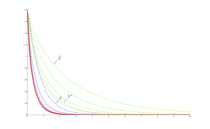
Figure 2: Computation of $\mathbb{E}\log\left(1+\left\|X_{t}\right\|^{2}\right)$, where $t\in\left[0,10\right]$ and $X_{t}$ solves (15). Dashed line: $V_{n}$, dashdot line: $\tilde{Z}$, dotted line: $Y^{s}$, and solid line: reference values. Here, $\Delta$ is equal to $1/8$, $1/16$, $1/32$ and $1/64$; smaller discretization steps produce better approximations.

Figure 2 shows the computation $\mathbb{E}\log\left(1+\left\|X_{t}\right\|^{2}\right)$ by means of $V_{n}$ (dashed line), $Y^{s}_{n}$ (dotted line), and the weak balanced scheme (dashdot line)

$$\widetilde{Z}_{n+1} =\widetilde{Z}_{n}+\begin{pmatrix}\sigma_{1}&0\\ 0&\sigma_{2}\end{pmatrix}\widetilde{Z}_{n}\sqrt{\Delta}\xi_{n}^{1}+\begin{pmatrix}0&-\epsilon\\ \epsilon&0\end{pmatrix}\widetilde{Z}_{n}\sqrt{\Delta}\xi_{n}^{2}$$

$$\quad+\sqrt{\Delta}\begin{pmatrix}\left|\sigma_{1}\right|+\left|\epsilon\right|&0\\ 0&\left|\sigma_{2}\right|+\left|\epsilon\right|\end{pmatrix}\left(\widetilde{Z}_{n}-\widetilde{Z}_{n+1}\right)$$

(see [3]). The reference values for $\mathbb{E}\log\left(1+\left\|X_{t}\right\|^{2}\right)$ (solid line) have been calculated by using the weak Euler method

$$\widetilde{Y}_{n+1}=\widetilde{Y}_{n}+\begin{pmatrix}\sigma_{1}&0\\ 0&\sigma_{2}\end{pmatrix}\widetilde{Y}_{n}\sqrt{\Delta}\,\xi_{n}^{1}+\begin{pmatrix}0&-\epsilon\\ \epsilon&0\end{pmatrix}\widetilde{Y}_{n}\sqrt{\Delta}\,\xi_{n}^{2}$$

with step-size $\Delta=2^{-13}\approx 0.000122$. Indeed, we plot the sample means obtained from $10^{8}$ trajectories of each scheme. Furthermore, Table 2 provides estimates of the errors $\epsilon\left(\hat{Y}\right):=\left|\mathbb{E}\log\left(1+\left\|X_{T}\right\|^{2}\right)-\mathbb{E}\log\left(1+\left\|\hat{Y}_{N}\right\|^{2}\right)\right|$, where $T=1,3$, $N=T/\Delta$, and $\hat{Y}_{n}$ represents the numerical methods $V_{n}$, $Y^{s}_{n}$, $\widetilde{Y}_{n}$ and $\widetilde{Z}_{n}$. From Table 2 we can see that $\widetilde{Y}_{n}$ blows up for $\Delta\leq 1/16$. Figure 2, together with Table 2, illustrate that $\widetilde{Z}_{n}$ is stable, but presents a slow rate of weak convergence. In contrast, the performance of $V_{n}$ is very good, $V_{n}$ mix good stability properties with reliable approximations. The heuristic balanced scheme $Y^{s}_{n}$ shows a very good behavior. In fact, the accuracy of $Y^{s}_{n}$ is very similar to that of $V_{n}$ for $\Delta\leq 1/16$, and $Y^{s}_{n}$ does not involve any optimization process.

		$\Delta$
		1/2	1/4	1/8	1/16	1/32	1/64
$\epsilon\left(\tilde{Y}\right)$	$T=1$	6.5497	9.4879	12.733	11.0676	0.15183	0.02365
	$T=3$	18.814	28.8744	38.9743	34.1327	0.0086188	0.00075718
$\epsilon\left(\tilde{Z}\right)$	$T=1$	1.3395	1.1777	0.98272	0.7757	0.58279	0.42137
	$T=3$	1.0611	0.78255	0.51624	0.30475	0.1643	0.08361
$\epsilon\left(Y^{s}\right)$	$T=1$	1.1914	0.85936	0.49789	0.15466	0.042484	0.018271
	$T=3$	0.81853	0.38585	0.10185	0.0096884	0.0013717	0.00055511
$\epsilon\left(V\right)$	$T=1$	1.2544	0.8482	0.36579	0.11998	0.029324	0.0069274
	$T=3$	0.64867	0.16695	0.035366	0.0065051	0.00068084	0.00031002

Table 2: Estimation of errors involved in the computation of $\mathbb{E}\log\left(1+\left\|X_{T}\right\|^{2}\right)$ for $T=1$ and $T=3$. Here, $X_{t}$ verifies (15) with $\sigma_{1}=7$, $\sigma_{2}=4$, $\epsilon=1$ and $X_{0}=\left(1,2\right)^{\top}$.

4 Proofs

Proof of Lemma 1.

We first prove that under Property P1, $\lim_{n\rightarrow\infty}Y^{s}_{n}=0$ $a.s.$ iff

$$\begin{cases}a\left(\Delta\right)<\left(\mu^{2}\Delta+2\mu-\lambda^{2}\right)/\left(2\mu\Delta\right),&\text{if }\mu<0\\ a\left(\Delta\right)\in\mathbb{R},&\text{if }\mu=0\text{ and }\lambda\neq 0\\ a\left(\Delta\right)>\left(\mu^{2}\Delta+2\mu-\lambda^{2}\right)/\left(2\mu\Delta\right),&\text{if }\mu>0\end{cases}.$$ (16)

Suppose that Property P1 holds. Applying the strong law of large numbers and the law of iterated logarithm we obtain that $Y^{s}_{n}\rightarrow 0$ $a.s.$ as $n\rightarrow\infty$ iff

$$\mathbb{E}\log\left(1+\left(\mu\Delta+\lambda\sqrt{\Delta}\xi^{1}_{n}\right)/\left(1-a\left(\Delta\right)\Delta\right)\right)<0$$ (17)

(see, e.g., Lemma 5.1 of [8]). Since

$$\mathbb{E}\log\left(1+\frac{\mu\Delta+\lambda\sqrt{\Delta}\xi^{1}_{n}}{1-a\left(\Delta\right)\Delta}\right)=\frac{1}{2}\log\left(\left(1+\frac{\mu\Delta}{1-a\left(\Delta\right)\Delta}\right)^{2}-\frac{\lambda^{2}\Delta}{\left(1-a\left(\Delta\right)\Delta\right)^{2}}\right),$$

inequality (17) becomes $2\mu\left(1-a\left(\Delta\right)\Delta\right)+\mu^{2}\Delta-\lambda^{2}<0$, which is equivalent to (16). This establishes our first claim.

From the assertion of the first paragraph we get that Property P1, together with $\lim_{n\rightarrow\infty}Y^{s}_{n}=0$ $a.s.$, is equivalent to (a) $a\left(\Delta\right)\in\left]-\infty,\min\{p_{1},p_{3}\}\right[\cup\left]p_{2},p_{3}\right[$ for $\mu<0$; (b) $a\left(\Delta\right)\in\left]-\infty,p_{1}\right[\cup\left]p_{2},+\infty\right[$ for $\mu=0$ and $\lambda\neq 0$; and $a\left(\Delta\right)\in\left]p_{3},p_{1}\right[\cup\left]\max\{p_{2},p_{3}\},+\infty\right[$ for $\mu>0$. This gives the lemma, because $p_{1}<p_{3}$ (resp. $p_{2}>p_{3}$) whenever $\mu<0$ (resp. $\mu>0$). ∎

Proof of Theorem 2.

In case $\lambda\neq 0$, using differential calculus we obtain that the function $\Delta\mapsto\left(1-\left|\lambda\right|\sqrt{\Delta}+\mu\Delta\right)/\Delta$ attains its global minimum at $4/\lambda^{2}$. Then, for all $\Delta>0$ and $\lambda\in\mathbb{R}$ we have

$$\left(1-\left|\lambda\right|\sqrt{\Delta}+\mu\Delta\right)/\Delta\geq\mu-\lambda^{2}/4.$$ (18)

First, we suppose that $\mu\leq 0$ and $\alpha_{1}\left(\Delta\right)>1/4$. From (18) it follows that $p_{1}>\mu-\alpha_{1}\left(\Delta\right)\lambda^{2}$, which implies $a\left(\Delta\right)\in\left]-\infty,p_{1}\right[$. Second, if $\mu>0$ and $\Delta\geq 2/\mu$, then $a\left(\Delta\right)\in\left]p_{2},+\infty\right[$. Third, assume that $\mu>0$ and $\Delta<2/\mu$. Since $\mu>0$, for any $\Delta<\lambda^{2}/\mu^{2}$ we have $1-\left|\lambda\right|\sqrt{\Delta}+\mu\Delta<1$. Using $2\mu-\lambda^{2}<0$ we get $\lambda^{2}/\mu^{2}>2/\mu$, and so $p_{1}=\left(1-\left|\lambda\right|\sqrt{\Delta}+\mu\Delta\right)/\Delta$ whenever $\Delta<2/\mu$. Applying (18) gives $p_{1}>\mu-\alpha_{2}\left(\Delta\right)\lambda^{2}$, because $\alpha_{2}\left(\Delta\right)>1/4$. On the other hand, we have $p_{3}<\mu-\alpha_{2}\left(\Delta\right)\lambda^{2}$ if and only if $2\mu-\lambda^{2}<\mu\Delta\left(2\mu-4\alpha_{2}\left(\Delta\right)\lambda^{2}\right)/2$, which becomes

$$\frac{2}{\mu}>\Delta\left(1+\left(4\alpha_{2}\left(\Delta\right)-1\right)\frac{\lambda^{2}}{\lambda^{2}-2\mu}\right)$$ (19)

since $2\mu-\lambda^{2}<0$ and $\mu>0$. By $2/\mu>\Delta$, (19) holds in case $\alpha_{2}\left(\Delta\right)\leq 1/4+\left(\lambda^{2}-2\mu\right)\left(2-\mu\Delta\right)/\left(8\lambda^{2}\right)$. Then $p_{3}<\mu-\alpha_{2}\left(\Delta\right)\lambda^{2}$, hence $a\left(\Delta\right)\in\left]p_{3},p_{1}\right[$. Combining Lemma 1 with the above three cases yields Properties P1 and P2. ∎

Proof of Theorem 3.

From (11) it follows that

$$V_{n}=A_{n-1}\left(\Delta,M\left(\Delta\right)\right)A_{n-2}\left(\Delta,M\left(\Delta\right)\right)\cdots A_{0}\left(\Delta,M\left(\Delta\right)\right)V_{0}.$$

Since $\xi^{k}_{n}$ are bounded, $\sup_{x\in\mathbb{R}^{d},\left\|x\right\|=1}\mathbb{E}\log_{+}\left(\left\|A_{0}\left(\Delta,M\left(\Delta\right)\right)x\right\|\right)<\infty,$ where $\log_{+}\left(x\right)$ stands for the positive part of $\log\left(x\right)$. Hence, $\lim_{n\rightarrow\infty}\frac{1}{n}\log\left(\left\|V_{n}\right\|\right)$ exists whenever $V_{0}\neq 0$, and only dependents on $V_{0}$. Furthermore,

$$\lim_{n\rightarrow\infty}\frac{1}{n}\log\left(\left\|V_{n}\right\|\right)=\int_{\left\|x\right\|=1}\mathbb{E}\log\left(\left\|A_{0}\left(\Delta,M\left(\Delta\right)\right)x\right\|\right)\mu\left(dx\right),$$

with $\mu$ probability measure (see, e.g., Theorem $3.1$ of [18]). This gives (12). ∎

References

- [1] G. N. Milstein, E. Platen, H. Schurz, Balanced implicit methods for stiff stochastic systems, SIAM J. Numer. Anal. 35 (1998) 1010–1019.
- [2] J. Alcock, K. Burrage, A note on the Balanced method, BIT 46 (2006) 689–710.
- [3] H. Schurz, Convergence and stability of balanced implicit methods for systems of SDEs, Int. J. Numer. Anal. Model. 2 (2005) 197–220.
- [4] H. Schurz, Basic concepts of numerical analysis of stochastic differential equations explained by balanced implicit theta methods, in: M. Zili, D. V. Filatova (Eds.), Stochastic Differential Equations and Processes, Springer, New York, 2012, pp. 1–139.
- [5] M. V. Tretyakov, Z. Zhang, A fundamental mean-square convergence theorem for SDEs with locally Lipschitz coefficients and its applications, SIAM J. Numer. Anal. 51 (2013) 3135–3162.
- [6] J. Alcock, K. Burrage, Stable strong order 1.0 schemes for solving stochastic ordinary differential equations, BIT 52 (2012) 539–557.
- [7] C. Kahl, H. Schurz, Balanced Milstein methods for ordinary SDEs, Monte Carlo Methods Appl. 12 (2006) 143–170.
- [8] D. J. Higham, Mean-square and asymptotic stability of the stochastic theta method, SIAM J. Numer. Anal. 38 (2000) 753–769.
- [9] D. J. Higham, X. Mao, C. Yuan, Almost sure and moment exponential stability in the numerical simulation of stochastic differential equations, SIAM J. Numer. Anal. 45 (2007) 592–609.
- [10] P. E. Kloeden, E. Platen, Numerical solution of stochastic differential equations, Springer-Verlag, Berlin, 1992.
- [11] P. H. Baxendale, A stochastic Hopf bifurcation, Probab. Theory Relat. Fields 99 (1994) 581–616.
- [12] I. Gyöngy, Approximations of stochastic partial differential equations, in: G. Da Prato, L. Tubaro (Eds.), Stochastic Partial Differential Equations, Vol. 227 of Lecture Notes in Pure and Appl. Math., Deker, New York, 2002, pp. 287–307.
- [13] A. Jentzen, P. Kloeden, Taylor approximations for stochastic partial differential equations, SIAM, Philadelphia, 2011.
- [14] R. Biscay, J. C. Jimenez, J. J. Riera, P. A. Valdes, Local linearization method for the numerical solution of stochastic differential equations, Ann. Inst. Statist. Math. 48 (1996) 631 –644.
- [15] H. De la Cruz Cancino, R. J. Biscay, J. C. Jimenez, Carbonell, T. F.; Ozaki, High order local linearization methods: an approach for constructing a-stable explicit schemes for stochastic differential equations with additive noise, BIT 50 (2010) 509–539.
- [16] C. Graham, D. Talay, Stochastic simulation and Monte Carlo methods. Mathematical foundations of stochastic simulation., Springer, Berlin, 2013.
- [17] G. N. Milstein, M. V. Tretyakov, Stochastic numerics for mathematical physics, Springer, Berlin, 2004.
- [18] J. E. Cohen, C. M. Newman, The stability of large random matrices and their products, Ann. Probab. 12 (1984) 283–310.