Differentially Private Convex Optimization with Piecewise
Affine Objectives

Abstract

Differential privacy is a recently proposed notion of privacy that provides strong privacy guarantees without any assumptions on the adversary. The paper studies the problem of computing a differentially private solution to convex optimization problems whose objective function is piecewise affine. Such problem is motivated by applications in which the affine functions that define the objective function contain sensitive user information. We propose several privacy preserving mechanisms and provide analysis on the trade-offs between optimality and the level of privacy for these mechanisms. Numerical experiments are also presented to evaluate their performance in practice.

1 Introduction

With the advance in real-time computing and sensor technology, a growing number of user-based cyber-physical systems start to utilize user data for more efficient operation. In power systems, for example, the utility company now has the capability of collecting near real-time power consumption data from individual households through advanced metering infrastructures in order to improve the demand forecast accuracy and facilitate the operation of power plants [1]. At the same time, however, individual customer is exposed to the risk that the utility company or a potential eavesdropper can learn about information that the customer did not intend to share, which may include marketable information such as the type of appliances being used or even sensitive information such as the customer’s daily activities. Concerns on such privacy issues have been raised [17] and start to become one major hindrance to effective user participation [10].

Unfortunately, it has been long recognized that ad-hoc solutions (e.g., anonymization of user data) are inadequate to guarantee privacy due to the presence of public side information. This fact has been demonstrated through various instances such as identification of Netflix subscribers in the anonymized Netflix prize dataset through linkage with the Internet Movie Database (IMDb) [18]. Providing rigorous solutions to preserving privacy has become an active area of research. In the field of systems engineering, recent work on privacy includes, among others, privacy-preserving filtering of streaming data [14], privacy in smart metering [20], privacy in traffic monitoring [3], privacy in stochastic control [23], etc.

Recently, the notion of differential privacy proposed by Dwork and her collaborators has received attention due to its strong privacy guarantees [7]. The original setting assumes that the sensitive database is held by a trustworthy party (often called curator in related literature), and the curator needs to answer external queries (about the sensitive database) that potentially come from an adversary who is interested in learning information belonging to some user. Informally, preserving differential privacy requires that the curator must ensure that the results of the queries remain approximately unchanged if data belonging to any single user in the database are modified or removed. In other words, the adversary knows little about any single user’s information from the results of queries. Interested readers can refer to recent survey papers on differential privacy for more details on this topic [6].

Aside from privacy, another important aspect to consider is the usefulness of the results of queries. In the context of systems operation, user data are often used for guiding decisions that optimize systems performance. Specifically, the “query” now becomes the solution to the optimization problem, whereas “user data” correspond to parameters that appear in the objective function and/or constraints of the optimization problem. It is conceivable that preserving user privacy will come at the cost of optimality. Indeed, without any considerations on systems performance, one could protect privacy by choosing to ignore user data, which may lead to solutions that are far from being optimal.

Several researchers have looked into the application of differential privacy to optimization problems. For example, Gupta et al. have studied differential privacy in combinatorial optimization problems and derived information-theoretic bounds on the utility for a given privacy level [9]. Among all related efforts, one that receives increasingly more attention is applying differential privacy to convex optimization problems. Convex optimization problems have traditionally been extensively studied due to the richness in related results in optimization theory and their broad applications. In the case of unconstrained convex optimization, which appears frequently in machine learning (e.g., regression problems), techniques such as output perturbation and objective perturbation have been proposed by, among others, Chaudhuri et al. [5] and Kifer et al. [13]. Huang et al. have studied the setting of private distributed convex optimization, where the cost function of each agent is considered private [12]. Very recently, Hsu et al. have proposed mechanisms for solving linear programs privately using a differentially private variant of the multiplicative weights algorithm [11].

Rather than focusing on general convex optimization problems or even linear programs, the work in this paper studies the class of convex optimization problems whose objective function is piecewise affine, with the possibility of including linear inequality constraints. This form of optimization problems arises in applications such as $\ell_{1}$/$\ell_{\infty}$-norm optimization and resource allocation problems. On one hand, focusing on this particular class of problems allows us to exploit special structures that may lead to better algorithms. On the other hand, such problems can be viewed as a special form of linear programs, and it is expected that studies on this problem may lead to insights into applying differential privacy to more general linear programs.

Our major result in this paper is the introduction and analysis of several mechanisms that preserve differential privacy for convex optimization problems of this kind. These mechanisms include generic mechanisms such as the Laplace mechanism and the exponential mechanism. We also propose a new mechanism named differentially private subgradient method, which obtains a differentially private solution by iteratively solving the problem privately. In addition, we provide theoretical analysis on the suboptimality of these mechanisms and show the trade-offs between optimality and privacy.

2 Problem statement

2.1 Differential privacy

Denote by $\mathcal{D}$ the universe of all databases of interest. The information that we would like to obtain from a database $D\in\mathcal{D}$ is represented by a mapping called query $q\colon\mathcal{D}\to\mathcal{Q}$ for some target domain $\mathcal{Q}$. When the database $D$ contains private user information, directly making $q(D)$ available to the public may cause users in the database to lose their privacy, and addition processing (called a mechanism) that depends on $q$ is generally necessary in order to preserve privacy.

Example 1.

For a database containing the salaries of a group of people, we can define $D=\{x_{i}\}_{i=1}^{n}$, where $x_{i}\in\mathbb{R}_{+}$ is the salary of user $i$ (assuming no minimum denomination). Suppose someone is interested in the average salary of people in the database. Then the query can be written as $q(D)=\sum_{i=1}^{n}x_{i}/n$ for the target domain $\mathcal{Q}=\mathbb{R}_{+}$.

The fundamental idea of differential privacy is to translate privacy of an individual user in the database into changes in the database caused by that user (hence the name differential). With this connection, preserving privacy becomes equivalent to hiding changes in the database. Basic changes include addition, removal, and modification of a single user’s data in the database: addition/removal is often used if privacy is the presence/participation of any single user in the database (which is common in surveys of diseases); modification is often used if privacy is in the user data record (if an adversary cannot tell whether the data record of any single user is modified, it is impossible for the adversary to obtain exact value of the data). More generally, changes in database can be defined by a symmetric binary relation on $\mathcal{D}\times\mathcal{D}$ called adjacency relation, which is denoted by $\mathrm{Adj}(\cdot,\cdot)$. It can be verified that addition, removal, or modification of data belonging to a single user defines a valid adjacency relation. We will use the the notion of adjacent database hereafter.

In the framework of differential privacy, all mechanisms under consideration are randomized, i.e., for a given database, the output of such a mechanism obeys a probability distribution. A differentially private mechanism must ensure that its output distribution does not vary much between two adjacent databases.

Definition 2 (Differential privacy [7]).

A randomized mechanism $M\colon\mathcal{D}\to\mathcal{Q}$ preserves $\epsilon$-differential privacy if for all $\mathcal{R}\subseteq\mathcal{Q}$ and all pairs of adjacent databases $D$ and $D^{\prime}$:

$$\mathbb{P}(M(D)\in\mathcal{R})\leq e^{\epsilon}\mathbb{P}(M(D^{\prime})\in\mathcal{R}).$$

The constant $\epsilon>0$ indicates the level of privacy: smaller $\epsilon$ implies higher level of privacy. The notion of differential privacy promises that an adversary cannot tell from the output with high probability whether data corresponding to a single user in the database have changed. This essentially hides user information at the individual level, no matter what side information an adversary may have. The necessity of randomized mechanisms is evident from the definition, since the output of any non-constant deterministic mechanism will normally change with the input database.

Remark 3.

One useful interpretation of differential privacy can be made in the context of detection theory [24, 8]. Suppose privacy is defined as user participation in the database and thus the adjacency relation is defined as addition/removal of a single user to/from the database. Consider an adversary who tries to detect whether a particular user $i$ is in the database from the output of an $\epsilon$-differentially private mechanism $M$ using the following rule: report true if the output of $M$ lies in some set $\mathcal{R}^{*}\subseteq\mathcal{Q}$ and false otherwise. Let $D$ be the database with user $i$ and $D^{\prime}$ be the one without. We are interested in the probabilities of two types of detection errors: false positive probability $p_{\mathrm{FP}}=\mathbb{P}(M(D^{\prime})\in\mathcal{R}^{*})$ (i.e., user $i$ is not present, but the detection algorithm reports true) and false negative probability $p_{\mathrm{FN}}=\mathbb{P}(M(D)\notin\mathcal{R}^{*})=\mathbb{P}(M(D)\in\mathcal{Q}\backslash\mathcal{R}^{*})$, both of which need to be small for achieving good detection. Since $D$ and $D^{\prime}$ are adjacent, we know from the definition of differential privacy that

$$\mathbb{P}(M(D)\in\mathcal{R}^{*}) \leq e^{\epsilon}\mathbb{P}(M(D^{\prime})\in\mathcal{R}^{*}),$$

$$\mathbb{P}(M(D^{\prime})\in\mathcal{Q}\backslash\mathcal{R}^{*}) \leq e^{\epsilon}\mathbb{P}(M(D)\in\mathcal{Q}\backslash\mathcal{R}^{*}),$$

which lead to

$$p_{\mathrm{FN}}+e^{\epsilon}p_{\mathrm{FP}}\geq 1\quad\text{and}\quad e^{\epsilon}p_{\mathrm{FN}}+p_{\mathrm{FP}}\geq 1.$$ (1)

The conditions in (1) imply that $p_{\mathrm{FN}}$ and $p_{\mathrm{FP}}$ cannot be both too small. Namely, these conditions limit the detection capability of the adversary so that the privacy of user $i$ is protected. For example, if $\epsilon=0.1$ and the false negative probability $p_{\mathrm{FN}}=0.05$, then the false positive probability $p_{\mathrm{FP}}\geq\max\{1-e^{\epsilon}p_{\mathrm{FN}},e^{-\epsilon}(1-p_{\mathrm{FN}})\}\approx 0.94$, which is quite large.

2.2 Problem statement

We consider minimization problems whose objective function $f\colon\mathbb{R}^{d}\to\mathbb{R}$ is convex and piecewise affine:

$$f(x)=\max_{i=1,2,\dots,m}\{a_{i}^{T}x+b_{i}\}$$ (2)

for some constants $\{a_{i}\in\mathbb{R}^{d},b_{i}\in\mathbb{R}\}_{i=1}^{m}$. For generality, we also add additional linear inequality constraints that define a convex polytope $\mathcal{P}$, so that the optimization problem has the following form:

$$\underset{x}{\mathrm{min.}}\quad f(x)\qquad\;\mathrm{s.t.}\quad x\in\mathcal{P}.$$ (3)

In this paper, we restrict our attention to the case where user information is in $\{b_{i}\}_{i=1}^{m}$, so that the database $D=\{b_{i}\}_{i=1}^{m}$. Any other information, including $\{a_{i}\}_{i=1}^{m}$ and $\mathcal{P}$, is considered as public and fixed. Define the adjacency relation between two databases $D=\{b_{i}\}_{i=1}^{m}$ and $D^{\prime}=\{b_{i}^{\prime}\}_{i=1}^{m}$ as follows:

$$\mathrm{Adj}(D,D^{\prime})\quad\text{if and only if}\quad\max_{i\in\{1,2,\dots,m\}}|b_{i}-b_{i}^{\prime}|\leq b_{\mathrm{max}}.$$ (4)

Since $D$ gives a complete description of problem (3), we will often use $D$ to represent both the database and the corresponding optimization problem. With the definition of adjacency relation, we are ready to give the formal problem statement.

Problem 4.

For all problems in the form of (3), find a mechanism $M$ that outputs an approximate optimal solution that preserves $\epsilon$-differential privacy under the adjacency relation (4). Namely, for all $\mathcal{R}\subseteq\mathcal{P}$ and all adjacent databases $D$ and $D^{\prime}$, the mechanism $M$ must satisfy

$$\mathbb{P}(M(D)\in\mathcal{R})\leq e^{\epsilon}\mathbb{P}(M(D^{\prime})\in\mathcal{R}).$$

2.3 Convex problems with piecewise affine objectives

In the following, we give several examples of convex minimization problems whose objective is piecewise affine:

Example 5 ($\ell_{\infty}$-norm).

The $\ell_{\infty}$-norm $f(x)=\left\|x\right\|_{\infty}$ can be rewritten in the form of (2) consisting of $2d$ affine functions:

$$f(x)=\max_{i=1,2,\dots,d}|x_{i}|=\max\{x_{1},-x_{1},x_{2},-x_{2},\dots,x_{d},-x_{d}\}.$$

Example 6 ($\ell_{1}$-norm).

The $\ell_{1}$-norm $f(x)=\left\|x\right\|_{1}$ can be rewritten in the form of (2) consisting of $2^{d}$ affine functions:

$$f(x)=\sum_{i=1}^{d}\max\{x_{i},-x_{i}\}=\max_{\{\alpha_{i}\in\{0,1\}\}_{i=1}^{d}}\sum_{i=1}^{d}(-1)^{\alpha_{i}}x_{i}.$$

Example 7 (Resource allocation).

Consider the following resource allocation problem, which is one such example where private optimal solution may be desired. Suppose we need to purchase a certain kind of resource and allocate it among $n$ agents, and we need to decide the optimal amount of resource to purchase. Agent $i$, if being allocated $z_{i}$ amount of resource, can provide utility $c_{i}z_{i}$, where $c_{i}$ is its utility gain. This holds until the maximum desired resource (denoted by $\bar{z}_{i}$) for agent $i$ is reached.

Suppose the total amount of resource to allocate is given as $x\geq 0$. The maximum utility gain can be determined by the optimal value of the following optimization problem

$$\underset{z}{\mathrm{max.}}\quad c^{T}z\qquad\;\mathrm{s.t.}\quad\mathbf{1}^{T}z\leq x,\qquad 0\preceq z\preceq\bar{z},$$ (5)

whose optimal value is denoted as $U(x)$. One can show that $U(x)$ is a concave and piecewise affine function by considering the dual of problem (5):

$$\underset{\lambda,\nu}{\mathrm{min.}}\quad \nu x+\lambda^{T}\bar{z}$$ (6)

$$\;\mathrm{s.t.}\quad \nu\geq 0,\qquad\lambda\succeq 0,\qquad\lambda+\nu\mathbf{1}-c\succeq 0.$$

Strong duality holds since the primal problem (5) is always feasible ($z=0$ is a feasible solution), which allows us to redefine $U(x)$ as the optimal value of problem (5). In addition, since the optimal value of any linear program can always be attained at a vertex of the constraint polytope, we can rewrite $U$ as the pointwise minimum of affine functions (hence $U$ is concave):

$$U(x)=\min_{i=1,2,\dots,m}\{\nu_{i}x+\lambda_{i}^{T}\bar{z}\},$$ (7)

where $\{(\nu_{i},\lambda_{i})\}_{i=1}^{m}$ are the vertices of the constraint polytope in problem (6). If we are interested in maximizing the net utility $U(x)-\mu x$ over $x$, where $\mu$ is the price of the resource, the problem becomes equivalent to one in the form of (3).

Remark 8.

In certain applications, the maximum desired resource $\bar{z}_{i}$, which is present in the affine functions in (7), may be treated as private information by agent $i$. As an example, consider the scenario where each agent represents a consumer in a power network, and the resource to be allocated is the available electricity. Then the maximum desired resource $\bar{z}_{i}$ can potentially reveal activities of consumer $i$, e.g., small $\bar{z}_{i}$ may indicate that consumer $i$ is away from home.

3 Useful tools in differential privacy

This section reviews several useful tools in differential privacy that will be used in later sections. Material in this section includes the (vector) Laplace mechanism, the exponential mechanism, the post-processing rule, and composition of private mechanisms. Readers who are familiar with these topics may skip this section.

When the range of query $\mathcal{Q}$ is $\mathbb{R}$, one commonly used differentially private mechanism is the Laplace mechanism [7]. In this paper, we use a multidimensional generalization of the Laplace mechanism for queries that lie in $\mathbb{R}^{d}$. Suppose the sensitivity of query $q$, defined as

$$\Delta:=\max_{D,D^{\prime}}\left\|q(D)-q(D^{\prime})\right\|_{\infty},$$

is bounded. Then one way to achieve $\epsilon$-differential privacy is to add i.i.d. Laplace noise $\mathrm{Lap}(d\Delta/\epsilon)$ to each component of $q$, which is guaranteed by the sequential composition theorem (Theorem 15) listed at the end of this section. However, a similar mechanism that requires less noise can be adopted in this case by using the fact that the $\ell_{2}$-sensitivity of the query $\Delta_{2}$ (defined below) is also bounded:

$$\Delta_{2}:=\max_{D,D^{\prime}}\left\|q(D)-q(D^{\prime})\right\|_{2}\leq\sqrt{d}\Delta.$$

Theorem 9.

For a given query $q$, let $\Delta_{2}=\max_{D,D^{\prime}}\left\|q(D)-q(D^{\prime})\right\|_{2}$ be the $\ell_{2}$-sensitivity of $q$. Then the mechanism $M(D)=q(D)+w$, where $w$ is a random vector whose probability distribution is proportional to $\exp(-\epsilon\left\|w\right\|_{2}/\Delta_{2})$, preserves $\epsilon$-differential privacy.

We are not aware of the name of the mechanism described in Theorem 9. Although the additive perturbation $w$ in Theorem 9 does not follow the Laplace distribution (in fact, it follows the Gamma distribution), we will still refer to this mechanism as the vector Laplace mechanism due to its close resemblance to the (scalar) Laplace mechanism.

Another useful and quite general mechanism is the exponential mechanism. This mechanism requires a scoring function $u\colon\mathcal{Q}\times\mathcal{D}\to\mathbb{R}$. For a given database $D$, the scoring function $u$ characterizes the quality of any candidate query: if a query $q$ is more desirable than another query $q^{\prime}$, then we have $u(D,q)>u(D,q^{\prime})$. The exponential mechanism $M_{E}(D;u)$ guarantees $\epsilon$-differential privacy by randomly reporting $q$ according to the probability density function

$$\frac{\exp(\epsilon u(D,q)/2\Delta_{u})}{\int_{q^{\prime}\in\mathcal{Q}}\exp(\epsilon u(D,q^{\prime})/2\Delta_{u})\,dq^{\prime}},$$

where

$$\Delta_{u}:=\max_{x}\max_{D,D^{\prime}\colon\mathrm{Adj}(D,D^{\prime})}|u(D,x)-u(D^{\prime},x)|$$

is the (global) sensitivity of the scoring function $u$.

Theorem 10 (McSherry and Talwar [15]).

The exponential mechanism is $\epsilon$-differentially private.

When the range $\mathcal{Q}$ is finite, i.e., $|\mathcal{Q}|<\infty$, the exponential mechanism has the following probabilistic guarantee on the suboptimality with respect to the scoring function.

Theorem 11 (McSherry and Talwar [15]).

Consider the exponential mechanism $M_{E}(D;u)$ acting on a database D under a scoring function $u$. If $\mathcal{Q}$ is finite, i.e., $|\mathcal{Q}|<\infty$, then $M_{E}$ satisfies

$$\mathbb{P}\left[u_{\mathrm{opt}}-u(D,M_{E}(D;u))\geq\frac{2\Delta_{u}}{\epsilon}(\log|\mathcal{Q}|+t)\right]\leq e^{-t},$$

where $u_{\mathrm{opt}}=\max_{q\in\mathcal{Q}}u(D,q)$.

It is also possible to obtain the expected suboptimality using the following lemma.

Lemma 12.

Suppose a random variable $X$ satisfies: (1)$X\geq 0$ and (2) $\mathbb{P}(X\geq t)\leq e^{-\alpha t}$ for some $\alpha>0$. Then it holds that $\mathbb{E}[X]\leq 1/\alpha$.

Proof.

Use the fact that $X\geq 0$ to write $X=\int_{0}^{\infty}I(X\geq t)\,dt.$ Then

$$\mathbb{E}[X]=\mathbb{E}\left[\int_{0}^{\infty}I(X\geq t)\,dt\right]=\int_{0}^{\infty}\mathbb{E}[I(X\geq t)]\,dt=\int_{0}^{\infty}\mathbb{P}(X\geq t)\,dt\leq\int_{0}^{\infty}e^{-\alpha t}\,dt=1/\alpha.$$

∎

Combine Theorem 11 and Lemma 12 to obtain the expected suboptimality.

Theorem 13.

Under the same assumptions in Theorem 11, the exponential mechanism $M_{E}(D;u)$ satisfies

$$\mathbb{E}\left[u_{\mathrm{opt}}-u(D,M_{E}(D;u))\right]\leq 2\Delta_{u}(1+\log|\mathcal{Q}|)/\epsilon.$$

Finally, there are two very useful theorems that enable construction of new differentially private mechanisms from existing ones.

Theorem 14 (Post-processing).

Suppose a mechanism $M\colon\mathcal{D}\to\mathcal{Q}$ preserves $\epsilon$-differential privacy. Then for any function $f$, the (functional) composition $f\circ M$ also preserves $\epsilon$-differential privacy.

Theorem 15 (Seqential composition [16]).

Suppose a mechanism $M_{1}$ preserves $\epsilon_{1}$-differential privacy, and another mechanism $M_{2}$ preserves $\epsilon_{2}$-differential privacy. Define a new mechanism $M(D):=(M_{1}(D),M_{2}(D))$. Then the mechanism $M$ preserves $(\epsilon_{1}+\epsilon_{2})$-differential privacy.

4 Privacy-preserving mechanisms

This section presents the main theoretical results of this paper. In particular, we propose several mechanisms that are able to obtain a differentially private solution to Problem 4. We also give suboptimality analysis for most mechanisms and show the trade-offs between optimality and privacy.

4.1 The Laplace mechanism acting on the problem data

One straightforward way of preserving differential privacy is to obtain the optimal solution from a privatized version of problem (3) by publishing the entire database $D$ privately using the vector Laplace mechanism described in Theorem 9. Privacy is guaranteed by the post-processing rule: once the problem is privatized, obtaining the optimal solution can be viewed as post-processing and does not change the level of privacy due to Theorem 14.

Theorem 16.

The mechanism that outputs $M_{P}(b)=b+w_{P}$, where $w_{P}$ is drawn from the probability density function that is proportional to $\exp(-\epsilon\left\|w_{P}\right\|_{2}/\sqrt{m}b_{\max})$, is $\epsilon$-differentially private.

Proof.

In this case, the query is $b$, whose $\ell_{2}$-sensitivity can be obtained as $\Delta=\max_{b,b^{\prime}}\left\|b-b^{\prime}\right\|_{2}=\sqrt{m}b_{\mathrm{max}}.$ Combining with Theorem 9 completes the proof. ∎

4.2 The Laplace mechanism acting on the problem solution

Another way of preserving differential privacy is to apply the vector Laplace mechanism directly on the optimal solution $x_{\mathrm{opt}}(D)$ of the problem: $M_{S}(D)=x_{\mathrm{opt}}(D)+w_{S}$. The additive noise $w_{S}$ is drawn from the distribution proportional to $\exp(-\epsilon\left\|w_{S}\right\|_{2}/\sqrt{d}\Delta)$, where $\Delta$ is the sensitivity of the optimal solution, i.e.,

$$\Delta=\max_{D,D^{\prime}\colon\mathrm{Adj}(D,D^{\prime})}\left\|x_{\mathrm{opt}}(D)-x_{\mathrm{opt}}(D^{\prime})\right\|_{2}.$$

This mechanism is $\epsilon$-differentially private also due to Theorem 9.

Unfortunately, it is generally difficult to analyze how the optimal solution $x_{\mathrm{opt}}(D)$ changes with $D$, and hence the exact value of $\Delta$ is often unavailable. However, when the set $\mathcal{P}$ is compact, an upper bound of $\Delta$ can be given by the diameter of $\mathcal{P}$, defined as $\mathrm{diam}(\mathcal{P}):=\max_{x,y\in\mathcal{P}}\left\|x-y\right\|_{2}.$ Although $\mathrm{diam}(\mathcal{P})$ is still difficult to compute for a generic set $\mathcal{P}$, there are several cases where its exact value or an upper bound can be computed efficiently. One simple case is when $\mathcal{P}=\{x\colon 0\leq x_{i}\leq 1,\>i=1,2,\dots,d\}$ is a hypercube and hence $\mathrm{diam}(\mathcal{P})=\sqrt{d}$. In the more general case where $\mathcal{P}$ is described by a set of linear inequalities, an upper bound can be obtained by computing the longest axis of the Löwner-John ellipsoid of $\mathcal{P}$, i.e., the minimum-volume ellipsoid that covers $\mathcal{P}$. The Löwner-John ellipsoid can be approximated from the maximum-volume inscribed ellipsoid, which can be obtained by solving a convex optimization problem (in particular, a semidefinite problem, cf. [2, page 414] ).

Suboptimality analysis for this mechanism is given by the following theorem.

Theorem 17.

Define $G=\max_{i}\left\|a_{i}\right\|_{2}$. The expected suboptimality for the solution perturbation mechanism $M_{S}$ is bounded as

$$\mathbb{E}[f(M_{S}(D))-f(x_{\mathrm{opt}})]\leq Gd^{3/2}\Delta/\epsilon.$$

Proof.

Since $f(x)-f(x_{\mathrm{opt}})\geq 0$ for all $x\in\mathcal{P}$, we have

$$\mathbb{E}[f(M_{S}(D))-f(x_{\mathrm{opt}})]=\mathbb{E}|f(M_{S}(D))-f(x_{\mathrm{opt}})|.$$

It is not difficult to show that $f$ is Lipschitz with $G$ as the Lipschitz constant, i.e., $|{\normalcolor f(x)-f(y)|}\leq G\left\|x-y\right\|_{2},$which leads to

$$\mathbb{E}[f(M_{S}(D))-f(x_{\mathrm{opt}})]\leq G\mathbb{E}\left\|M_{S}(D)-x_{\mathrm{opt}}\right\|_{2}=G\mathbb{E}\left\|w_{S}\right\|_{2}=Gd\cdot\sqrt{d}\Delta/\epsilon=Gd^{3/2}\Delta/\epsilon.$$

∎

Theorem 17 shows that the expected suboptimality grows as $\epsilon$ decreases (i.e., the level of privacy increases). The suboptimality also grows with $d$, which is the dimension of the decision variable $x$.

4.3 The exponential mechanism

To use the exponential mechanism for privately solving minimization problems, one natural choice of the scoring function is the negative objective function $-f$. However, this choice may not work in all cases, since changes in user data can lead to an infeasible problem, which yields unbounded sensitivity. Even when the problem remains feasible, the sensitivity of the objective function with respect to data can be difficult to compute for a generic optimization problem. Nevertheless, the following shows that the sensitivity for our problem is bounded and can be computed exactly.

Lemma 18.

Suppose the scoring function is given as

$$u(x,D) =-f(x,D)=-\max_{i=1,2,\dots,m}\{a_{i}^{T}x+b_{i}\}.$$

Then the sensitivity of $u$ for the adjacency relation defined in (4) is $\Delta_{u}=b_{\max}$.

Proof.

See Appendix A.1. ∎

As a result of Theorem 10 and Lemma 18, we know that we can achieve $\epsilon$-differential privacy by using the exponential mechanism given in the following theorem.

Theorem 19.

The exponential mechanism $M_{E}$, which randomly outputs $\tilde{x}_{\mathrm{opt}}$ according the probability density function

$$\frac{\exp(-\epsilon f(\tilde{x}_{\mathrm{opt}},D)/2b_{\max})}{\int_{x\in\mathcal{P}}\exp(-\epsilon f(x,D)/2b_{\max})\,dx},$$ (8)

is $\epsilon$-differentially private.

Remark 20.

The denominator in (8) needs to remain bounded in order for (8) to be a valid probability distribution. This trivially holds when $\mathcal{P}$ is bounded. When $\mathcal{P}$ is unbounded, this can be shown by using the fact that $f(x,D)$ is affine in $x$ and the integrand decreases exponentially fast as $\left\|x\right\|\to\infty$.

Suboptimality analysis for the exponential mechanism is given by the following theorem.

Theorem 21.

The expected suboptimality for the exponential mechanism $M_{E}$ is bounded as

$$\mathbb{E}[f(M_{E}(D))-f_{\mathrm{opt}}]\leq C(0,\epsilon)\cdot 2b_{\max}/\epsilon,$$

where $f_{\mathrm{opt}}=\min_{x\in\mathcal{P}}f(x,D)$ and for any $\gamma\geq 0$,

$$C(\gamma,\epsilon)=\frac{\exp(-\epsilon f_{\mathrm{opt}}/2b_{\max})\int_{x\colon f(x,D)\geq f_{\mathrm{opt}}+\gamma}\,dx}{\int_{x\in\mathcal{P}}\exp(-\epsilon f(x,D)/2b_{\max})\,dx}.$$

Proof.

We first prove that for any $\gamma\geq 0$,

$$\mathbb{P}[f(M_{E}(D))-f_{\mathrm{opt}}\geq\gamma]\leq C(\gamma,\epsilon)\exp(-\epsilon\gamma/2b_{\max}).$$ (9)

For any given $a\in\mathbb{R}$, the exponential mechanism $M_{E}(D)$ with scoring function $u$ satisfies

$$\mathbb{P}[u(M_{E}(D))\leq a] =\frac{\int_{x:u(x,D)\leq a}\exp(\epsilon u(x,D)/2b_{\max})\,dx}{\int_{x\in\mathcal{P}}\exp(\epsilon u(x,D)/2b_{\max})\,dx}$$

$$\leq\frac{\exp(\epsilon a/2b_{\max})\int_{x:u(x,D)\leq a}\,dx}{\int_{x\in\mathcal{P}}\exp(\epsilon u(x,D)/2b_{\max})\,dx}.$$

Set $u(x,D)=-f(x,D)$ and $a=-(\gamma+f_{\mathrm{opt}})$ to obtain (9).

Note that $C(\gamma,\epsilon)\leq C(0,\epsilon)$ for all $\gamma\geq 0$. Then

$$\mathbb{P}[f(M_{E}(D))-f_{\mathrm{opt}}\geq\gamma]\leq C(0,\epsilon)\exp(-\epsilon\gamma/2b_{\max}).$$ (10)

Apply Lemma 12 on (10) to complete the proof. ∎

It can be shown that $C(0,\epsilon)$ increases as $\epsilon$ decreases. Therefore, similar to the solution perturbation mechanism $M_{S}$ described in Theorem 17, the expected suboptimality of $M_{E}$ grows as $\epsilon$ decreases.

4.4 Private subgradient method

If privacy is not a concern, one way to solve the optimization problem (3) is to use the subgradient method, which iteratively searches for an optimal solution by moving along the direction of a subgradient. Although the direction of a subgradient is not necessarily a descent direction, the subgradient method is still guaranteed to converge if one keeps track of the best (rather than the most recent) solution among all past iterations. Recall that $g$ is a subgradient of $f$ at $x_{0}$ if and only if for all $x$:

$$f(x)\geq f(x_{0})+g^{T}(x-x_{0}).$$ (11)

For a convex and piecewise affine function $f$, its subgradient at any given $x_{0}$ can be obtained as follows. First find $k\in\{1,2,\dots,m\}$ such that

$$a_{k}^{T}x_{0}+b_{k}=\max_{i=1,2,\cdots,m}\{a_{i}^{T}x_{0}+b_{i}\}.$$ (12)

Then a subgradient at $x_{0}$ is $a_{k}$, which can be verified using the definition (11).

It can be seen from (12) that computing subgradients requires access to the private data $\{b_{i}\}_{i=1}^{m}$. Following from Hsu et al. [11], in order to preserve privacy when applying any iterative method (such as the subgradient method), one must make sure to: (1) privatize the computation during each iteration; (2) limit the total number of iterations.

One method for obtaining a subgradient privately is to perturb the true subgradient by adding, e.g., Laplace noise [22]. In our case, since the candidate subgradients come from a finite set $\{a_{i}\}_{i=1}^{m}$, we propose to use the exponential mechanism to privatize the computation of subgradients. Choose the scoring function $u_{\mathrm{sub}}\colon\{1,2,\cdots,m\}\to\mathbb{R}$ as $u_{\mathrm{sub}}(i;x,D)=a_{i}^{T}x+b_{i}$ (in the following, we will sometimes drop $D$ for conciseness). The sensitivity of $u_{\mathrm{sub}}$ at any given $x_{0}$, which is denoted as $\Delta_{u_{\mathrm{sub}}}(x_{0})$, can be computed as

$$\max_{i\in\{1,2,\dots,m\}}\max_{D,D^{\prime}}|u_{\mathrm{sub}}(i;x_{0},D)-u_{\mathrm{sub}}(i;x_{0},D^{\prime})|=b_{\max}.$$

1. Choose the scoring function $u\colon\{1,2,\cdots,m\}\to\mathbb{R}$ as

   $$u_{\mathrm{sub}}(i;x_{0})=a_{i}^{T}x_{0}+b_{i}.$$

2. Select the index $i^{*}$ using the exponential mechanism:

   $$\mathbb{P}(i^{*}=i)\propto\exp(-\epsilon u_{\mathrm{sub}}(i;x_{0})/2b_{\max}).$$

3. Output $a_{i^{*}}$ as the approximate subgradient at $x_{0}$.

Algorithm 1 $\epsilon$-differentially private subgradient.

If the subgradient computation in the regular subgradient method is replaced by Algorithm 1, the modified subgradient method (Algorithm 2) can be shown to preserve $\epsilon$-differential privacy using the sequential composition theorem, since each iteration preserves $(\epsilon/k)$-differential privacy and the total number of iterations is $k$.

1. Choose the number of iterations $k$, step sizes $\{\alpha_{i}\}_{i=1}^{k}$, and $x^{(1)}\in\mathcal{P}$.

2. For $i=1,2,\dots,k$, repeat:

   1. Obtain an $(\epsilon/k$)-private subgradient $g^{(i)}$ using Algorithm 1;

   2. Update $x^{(i+1)}:=x^{(i)}-\alpha_{i}g^{(i)}.$

3. Output $x^{(k+1)}$ as the solution.

Algorithm 2 $\epsilon$-differentially private subgradient method.

However, since the output of Algorithm 1 does not correspond to a true subgradient, it is natural to ask how this affects convergence of the optimization procedure. For any given $x_{0}$, define

$$\gamma(j;x_{0}) :=\max_{i\in\{1,2,\dots,m\}}u_{\mathrm{sub}}(i;x_{0})-u_{\mathrm{sub}}(j;x_{0})$$

$$=\max_{i=1,2,\dots,m}\{a_{i}^{T}x_{0}+b_{i}\}-(a_{j}^{T}x_{0}+b_{j}),$$

which is the suboptimality gap of choosing $a_{j}$ (in Algorithm 1) measured by the scoring function $u_{\mathrm{sub}}$. As a consequence of using the exponential mechanism in step 2 of Algorithm 1, an upper bound on the expectation of $\gamma$ can be obtained using Theorem 13:

$$\mathbb{E}_{i^{*}}[\gamma(i^{*};x_{0})]\leq 2b_{\max}(1+\log m)/\epsilon.$$ (13)

The following lemma shows how the suboptimality gap $\gamma$ affects the subgradient condition (11) if $a_{j}$ is used as a subgradient.

Lemma 22.

For all $x$, it holds that

$$f(x)\geq f(x_{0})+a_{j}^{T}(x-x_{0})-\gamma(j;x_{0}).$$

Proof.

We have

$$f(x) =\max_{i=1,2,\dots,m}\{a_{i}^{T}x+b_{i}\}$$

$$\geq a_{j}^{T}x+b_{j}$$

$$=(a_{j}^{T}x_{0}+b_{j})+a_{j}^{T}(x-x_{0})$$

$$=\max_{i=1,2,\dots,m}\{a_{i}^{T}x_{0}+b_{i}\}-\gamma(j;x_{0})+a_{j}^{T}(x-x_{0})$$

$$=f(x_{0})+a_{j}^{T}(x-x_{0})-\gamma(j;x_{0}).$$

∎

Remark 23.

If $j=\arg\max_{i\in\{1,2,\dots,m\}}u_{\mathrm{sub}}(i;x_{0})$, i.e., $a_{j}$ is a true subgradient, then Lemma 22 recovers the original definition of subgradient:

$$f(x)\geq f(x_{0})+a_{j}^{T}(x-x_{0}).$$

Lemma 22 shows that the suboptimality gap $\gamma$ also characterizes the extent that the subgradient condition is violated. Now we are ready to show the expected suboptimality of the differentially private subgradient method using both the bound (13) on $\mathbb{E}_{i^{*}}[\gamma(i^{*};x_{0})]$ and Lemma 22.

Theorem 24.

When the $\epsilon$-differentially private subgradient method is applied, the expected suboptimality after $k$ iterations is bounded as

$$\mathbb{E}\left[\min_{i=1,2,\dots,k}f(x^{(i)})-f_{\mathrm{opt}}\right]\leq\frac{R^{2}+G^{2}\sum_{i=1}^{k}\alpha_{i}^{2}}{2\sum_{i=1}^{k}\alpha_{i}}+\bar{\gamma}(\epsilon/k),$$ (14)

where $R=\mathrm{diam}(\mathcal{P})$, $G=\max_{i=1,2,\dots,m}\left\|a_{i}\right\|_{2}$, and $\bar{\gamma}(z)=2b_{\max}(1+\log m)/z$.

Proof.

See Appendix A.2. ∎

Theorem 24 shows a tradeoff between privacy and suboptimality. The first term, which also appears in the convergence analysis for the regular subgradient method, implies that the optimal gap vanishes as the number of iterations $k\to\infty$. However, if $k$ becomes too large, inaccuracy in the private subgradients will start to act as a dominant factor in suboptimality as the second term indicates. In particular, Theorem 24 implies that there exists an optimal number of iterations: as the number of iterations grows, the first term in (14) decreases, whereas $\bar{\gamma}(\epsilon/k)$ increases due to increased level of privacy for each iteration. Similar to previous results given by Theorem 17 and 21, the second term (due to privacy) grows as $\epsilon$ decreases.

5 Numerical experiments

5.1 Implementation details

In all simulations, the problem data $\{(a_{i},b_{i})\}_{i=1}^{m}$ are generated from i.i.d. Gaussian distributions. The constraint set is chosen to be a $d$-dimensional hypercube centered at the origin: $\mathcal{P}=\{x\colon-c\preceq x\preceq c\},$ whose diameter $\mathrm{diam}(\mathcal{P})=2\sqrt{d}c$. The level of privacy $\epsilon$ is set at $0.1$. The expected objective value for different privacy-preserving mechanisms is approximated by the sample average from $1000$ runs.

Implementation of the vector Laplace noise

One way to efficiently generate $w$ from the distribution proportional to $\exp(-\lambda\left\|w\right\|_{2})$ is to draw its magnitude $\bar{w}$ and direction $\hat{e}$ (as a unit vector) separately. It can be shown that $\bar{w}$ follows the Gamma distribution $\Gamma(d,\lambda)$ and the distribution of $\hat{e}$ is isotropic [4]. In order to draw a sample from $\Gamma(d,\lambda)$, one can draw $d$ i.i.d. samples $w_{1},w_{2},\dots,w_{d}$ from the exponential distribution: $w_{i}\sim\lambda\exp(-\lambda w_{i})$ $(w_{i}\geq 0)$ and obtain $\bar{w}=\sum_{i=1}^{d}w_{i}$. The direction $\hat{e}$ can be generated by drawing from the $d$-dimensional standard Gaussian distribution followed by normalization.

Implementation of the exponential mechanism

The exponential mechanism requires drawing samples from a distribution proportional to a non-negative function. Such sampling is usually performed using Markov chain Monte Carlo (MCMC) methods [19], which draw samples by simulating a Markov chain whose stationary distribution is the target distribution. In this paper, we use the Metropolis algorithm with a multivariate Gaussian proposal distribution. Due the shape of the constraint set, the covariance matrix $\Sigma$ of the Gaussian distribution is chosen to be isotropic, and its magnitude is set to be proportional to the size of the constraint set: $\Sigma=\eta cI_{d\times d}$, where $I_{d\times d}$ is the $d\times d$ identity matrix, and $\eta=0.1$. Each sample is generated by running $5000$ MCMC steps, after which the Markov chain is considered to have reached its stationary distribution.

Number of iterations for the subgradient method

Although Theorem 24 clearly shows that an optimal number of iterations exists for a given choice of $\epsilon$, the suboptimality bound is often loose for a given problem so that optimizing the bound does not provide direct guidance for choosing the number of iterations. In practice, we observe that the objective value is quite robust to the number of iterations, as shown in Fig. 1. The plot also includes the objective values obtained from the regular subgradient method, which decrease slightly as the number of iteration grows. Due to this robustness, in all subsequent simulations, the number of iterations is fixed at $100$.

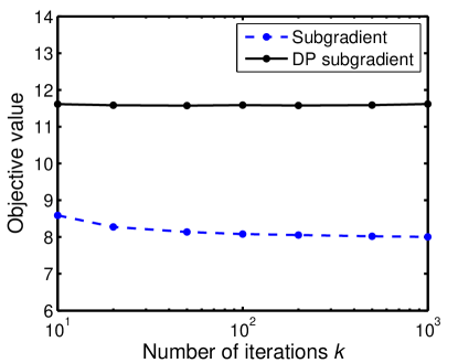
Figure 1: Objective values as a function of the number of iterations. Blue: Objective values obtained from the regular subgradient method. Black: Objective values obtained from the differentially private subgradient method.

5.2 Results and discussions

The simulations investigate the effects of changing $c$ (the size of the constraint set $\mathcal{P}$) and $m$ (the number of member affine functions) on all the mechanisms presented in Section 4. Fig. 2 shows the expected objective value as a function of $c$ as well as the true optimal value obtained by solving the original problem. For all privacy preserving mechanisms, the expected optimal value eventually grows as $c$ increases, except that it shows some initial decrease for the exponential mechanism and the differentially private subgradient method. This non-monotonic behavior can be explained by noticing two factors that contribute to the objective value. One factor is the effect of $c$ on the (original) optimization problem itself. As $c$ increases, it leads to a more relaxed optimization problem and consequently decreases the true optimal value (magenta dashed line). Another factor of $c$ is on the amount of perturbation introduced by the mechanisms. For example, for the mechanism that perturbs the solution directly, the magnitude of the vector Laplace noise grows with $c$. For the exponential mechanism, the distribution from which the solution is drawn will become less concentrated around the optimal solution as $c$ grows. We are unable to provide a definitive explanation for the other two mechanisms, but it is expected that changes in $c$ have a similar effect.

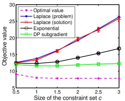
Figure 2: Objective values (with error bars corresponding to $2\sigma$ error) as a function of $c$ (the size of the constraint set $\mathcal{P}$) for different mechanisms. The true optimal value is shown for comparison.

The effect of $m$ on the objective value is illustrated in Fig. 3. As $m$ increases, more affine functions will be added (i.e., the affine functions used for a smaller $m$ is a subset of those used for a larger $m$). Unlike changing $c$, increasing $m$ causes the objective value to monotonically increase. First of all, adding more affine functions causes the optimal value (magenta dashed line) to increase even in the absence of privacy constraints. In addition, at least for the case when the problem is perturbed, the magnitude of the vector Laplace noise grows with $m$. For the differentially subgradient method, increase in $m$ also causes the suboptimality gap $\bar{\gamma}$ (that has $\log m$ dependence) to increase.

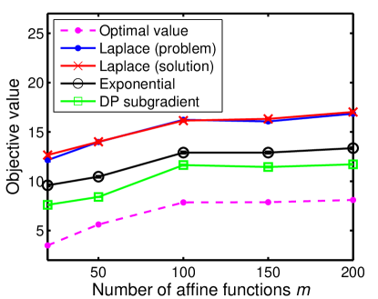
Figure 3: Objective values (with error bars corresponding to $2\sigma$ error) as a function of $m$ (the number of member affine functions) for different mechanisms. The true optimal value is shown for comparison.

As an interesting observation from all simulations, the differentially subgradient method is superior to other mechanisms. It achieves the lowest expected suboptimality among all mechanisms. Also, when $c$ increases, it has the slowest growth rate of suboptimality. The reason that why subgradient method works best is not evident from the suboptimality analysis presented in Section 4. It is known that the subgradient method is quite robust to unbiased noise in subgradients (often known as the stochastic subgradient method). However, in this work, the noise introduced by the exponential mechanism in Algorithm 1 is biased so that the analysis on stochastic subgradient method does not directly apply. This remains a interesting question for future investigations.

6 Conclusions

In this paper, we study the problem of preserving differential privacy for the solution of convex optimization problems with a piecewise affine objective. Several privacy-preserving mechanisms are presented, including the Laplace mechanism applied on either the problem data or the problem solution, the exponential mechanism, and the differentially private subgradient method. Theoretical analysis on the suboptimality of these mechanisms shows the trade-offs between optimality and privacy: more privacy can be provided at the expense of sacrificing optimality. Empirical numerical experiments show that the differentially private subgradient method has the least adverse effect on optimality for a given level of privacy. In addition, it is likely that the scheme of providing privacy by iteratively solving an optimization problem privately (as used by the private subgradient method) can be applied to more general convex optimization problems beyond the specific form studied in this paper. This appears to be an interesting direction for future investigations.

Acknowledgments. The authors would like to thank Aaron Roth for providing early access to the draft on differentially private linear programming [11] and helpful discussions on differential privacy. This work was supported in part by the NSF (CNS-1239224) and TerraSwarm, one of six centers of STARnet, a Semiconductor Research Corporation program sponsored by MARCO and DARPA.

Appendix A Proofs

A.1 Proof of Lemma 18

Proof.

Fix $x$, $D$, and $D^{\prime}$, and consider the quantity

$$\bar{\Delta}_{u} =u(x,D^{\prime})-u(x,D)$$

$$=\max_{i=1,2,\dots,m}\{a_{i}^{T}x+b_{i}\}-\max_{i=1,2,\dots,m}\{a_{i}^{T}x+b_{i}^{\prime}\}.$$

Define

$$j=\arg\max_{i}\{a_{i}^{T}x+b_{i}\}\quad\text{and}\quad k=\arg\max_{i}\{a_{i}^{T}x+b_{i}^{\prime}\}.$$

Using the fact that $a_{j}^{T}x+b_{j}\geq a_{i}^{T}x+b_{i}$ for all $i\in\{1,2,\dots,m\}$, we have

$$\bar{\Delta}_{u} =(a_{j}^{T}x+b_{j})-(a_{k}^{T}x+b_{k}^{\prime})$$ (15)

$$\geq(a_{k}^{T}x+b_{k})-(a_{k}^{T}x+b_{k}^{\prime})=b_{k}-b_{k}^{\prime}.$$ (16)

Similarly, since $a_{k}^{T}x+b_{k}^{\prime}\geq a_{i}^{T}x+b_{i}^{\prime}$ for all $i\in\{1,2,\dots,m\}$, we have

$$\bar{\Delta}_{u}\leq(a_{j}^{T}x+b_{j})-(a_{j}^{T}x+b_{j}^{\prime})=b_{j}-b_{j}^{\prime}.$$ (17)

Combining (15) and (17) together yields

$$|\bar{\Delta}_{u}|\leq\max\{|b_{k}-b_{k}^{\prime}|,|b_{j}-b_{j}^{\prime}|\}.$$

This is due to the fact that if $\alpha\leq\gamma\leq\beta$ for any constants $\alpha$, $\beta$, and $\gamma$, then $|\gamma|\leq\max\{|\alpha|,|\beta|\}$. Maximizing $|\bar{\Delta}_{u}|$ over all possible adjacent pairs of $D$ and $D^{\prime}$ yields

$$\max_{D,D^{\prime}\colon\mathrm{Adj}(D,D^{\prime})}|\bar{\Delta}_{u}|=b_{\max}.$$ (18)

Since (18) holds for any $x$, we have

$$\Delta_{u}=\max_{x}\max_{D,D^{\prime}\colon\mathrm{Adj}(D,D^{\prime})}|u(x,D)-u(x,D^{\prime})|=\max_{x}\max_{D,D^{\prime}\colon\mathrm{Adj}(D,D^{\prime})}|\bar{\Delta}_{u}|=b_{\max}.$$

∎

A.2 Proof of Theorem 24

Proof.

The proof follows the same procedure as the convergence proof for the stochastic subgradient descent method (cf. [21]), except for the presence of additional terms that depend on $\mathbb{E}_{i^{*}}[\gamma(i^{*},x^{(k)})]$ due to violation of the subgradient condition (11).

At iteration $k$, we have

$$\|x^{(k+1)}-x_{\mathrm{opt}}\|_{2}^{2} =\|x^{(k)}-\alpha_{k}g^{(k)}-x_{\mathrm{opt}}\|_{2}^{2}$$

$$=\|x^{(k)}-x_{\mathrm{opt}}\|_{2}^{2}-2\alpha_{k}g^{(k)T}(x^{(k)}-x_{\mathrm{opt}})+\alpha_{k}^{2}\|g^{(k)}\|_{2}^{2}.$$

Take $\mathbb{E}(\cdot|x^{(k)})$ on both sides to obtain

$$\mathbb{E}\left(\left.\|x^{(k+1)}-x_{\mathrm{opt}}\|_{2}^{2}\right|x^{(k)}\right)$$

$$\qquad=\|x^{(k)}-x_{\mathrm{opt}}\|_{2}^{2}-2\alpha_{k}\mathbb{E}(g^{(k)T}(x^{(k)}-x_{\mathrm{opt}})|x^{(k)})+\alpha_{k}^{2}\mathbb{E}\left(\left.\|g^{(k)}\|_{2}^{2}\right|x^{(k)}\right).$$

Since $g^{(k)}$ is computed from Algorithm 1, we have

$$\mathbb{E}(g^{(k)T}(x^{(k)}-x_{\mathrm{opt}})|x^{(k)}) \geq f(x^{(k)})-f(x_{\mathrm{opt}})-\mathbb{E}_{i^{*}}[\gamma(i^{*},x^{(k)})]$$

$$\geq f(x^{(k)})-f_{\mathrm{opt}}-\bar{\gamma}(\epsilon/k),$$

where $i^{*}$ is defined in Algorithm 1. This leads to

$$\mathbb{E}\left(\left.\|x^{(k+1)}-x_{\mathrm{opt}}\|_{2}^{2}\right|x^{(k)}\right)$$

$$\qquad\leq\|x^{(k)}-x_{\mathrm{opt}}\|_{2}^{2}-2\alpha_{k}(f(x^{(k)})-f_{\mathrm{opt}}-\bar{\gamma}(\epsilon/k))+\alpha_{k}^{2}\mathbb{E}\left(\left.\|g^{(k)}\|_{2}^{2}\right|x^{(k)}\right).$$

Now take expectation with respect to $x^{(k)}$:

$$\mathbb{E}\|x^{(k+1)}-x_{\mathrm{opt}}\|_{2}^{2}$$

$$\qquad\leq\mathbb{E}\|x^{(k)}-x_{\mathrm{opt}}\|_{2}^{2}-2\alpha_{k}(\mathbb{E}f(x^{(k)})-f_{\mathrm{opt}}-\bar{\gamma}(\epsilon/k))+\alpha_{k}^{2}\mathbb{E}\|g^{(k)}\|_{2}^{2}.$$

Repeat this procedure to obtain

$$\mathbb{E}\|x^{(k+1)}-x_{\mathrm{opt}}\|_{2}^{2}$$

$$\qquad\leq\mathbb{E}\|x^{(1)}-x_{\mathrm{opt}}\|_{2}^{2}-2{\textstyle\sum_{i=1}^{k}}\alpha_{i}(\mathbb{E}f(x^{(i)})-f_{\mathrm{opt}}-\bar{\gamma}(\epsilon/k))+{\textstyle\sum_{i=1}^{k}}\alpha_{i}^{2}\mathbb{E}\|g^{(i)}\|_{2}^{2}.$$

Rearrange the above and use the concavity of element-wise minimum to obtain the suboptimality bound (14).∎

References

- [1] The Benefits of Smart Meters. http://www.cpuc.ca.gov/PUC/energy/Demand+Response/benefits.htm (retrieved: March 19, 2014).
- [2] S. P. Boyd and L. Vandenberghe. Convex Optimization. Cambridge University Press, 2004.
- [3] E. S. Canepa and C. G. Claudel. A framework for privacy and security analysis of probe-based traffic information systems. In ACM International Conference on High Confidence Networked Systems, pages 25–32, 2013.
- [4] K. Chaudhuri and C. Monteleoni. Privacy-preserving logistic regression. In NIPS, volume 8, pages 289–296, 2008.
- [5] K. Chaudhuri, C. Monteleoni, and A. D. Sarwate. Differentially private empirical risk minimization. The Journal of Machine Learning Research, 12:1069–1109, 2011.
- [6] C. Dwork. Differential privacy: A survey of results. In Theory and Applications of Models of Computation, pages 1–19. Springer, 2008.
- [7] C. Dwork, F. McSherry, K. Nissim, and A. Smith. Calibrating noise to sensitivity in private data analysis. In Theory of Cryptography, pages 265–284. Springer, 2006.
- [8] Q. Geng and P. Viswanath. The optimal mechanism in differential privacy. arXiv preprint arXiv:1212.1186, 2012.
- [9] A. Gupta, K. Ligett, F. McSherry, A. Roth, and K. Talwar. Differentially private combinatorial optimization. In ACM-SIAM Symposium on Discrete Algorithms, pages 1106–1125, 2010.
- [10] R. Hoenkamp, G. B. Huitema, and A. J. de Moor-van Vugt. Neglected consumer: The case of the smart meter rollout in the netherlands, the. Renewable Energy L. & Pol’y Rev., page 269, 2011.
- [11] J. Hsu, A. Roth, T. Roughgarden, and J. Ullman. Privately solving linear programs. arXiv preprint arXiv:1402.3631, 2014.
- [12] Z. Huang, S. Mitra, and N. Vaidya. Differentially private distributed optimization. arXiv preprint arXiv:1401.2596, 2014.
- [13] D. Kifer, A. Smith, and A. Thakurta. Private convex empirical risk minimization and high-dimensional regression. Journal of Machine Learning Research, 1:41, 2012.
- [14] J. Le Ny and G. Pappas. Differentially private filtering. IEEE Transactions on Automatic Control, 59(2):341–354, 2014.
- [15] F. McSherry and K. Talwar. Mechanism design via differential privacy. In IEEE Symposium on Foundations of Computer Science, pages 94–103, 2007.
- [16] F. D. McSherry. Privacy integrated queries: an extensible platform for privacy-preserving data analysis. In ACM SIGMOD International Conference on Management of Data, pages 19–30, 2009.
- [17] A. Molina-Markham, P. Shenoy, K. Fu, E. Cecchet, and D. Irwin. Private memoirs of a smart meter. In ACM Workshop on Embedded Sensing Systems for Energy-Efficiency in Building, 2010.
- [18] A. Narayanan and V. Shmatikov. How to break anonymity of the netflix prize data set. The University of Texas at Austin, 2007.
- [19] W. H. Press, S. A. Teukolsky, W. T. Vetterling, and B. P. Flannery. Numerical Recipes: The Art of Scientific Computing. Cambridge University Press, 3rd edition, 2007.
- [20] L. Sankar, S. Rajagopalan, S. Mohajer, and H. Poor. Smart meter privacy: A theoretical framework. IEEE Transactions on Smart Grid, 4(2):837–846, 2013.
- [21] N. Z. Shor. Nondifferentiable optimization and polynomial problems, volume 24. Springer, 1998.
- [22] S. Song, K. Chaudhuri, and A. D. Sarwate. Stochastic gradient descent with differentially private updates. In IEEE Global Conference on Signal and Information Processing, 2013.
- [23] P. Venkitasubramaniam. Privacy in stochastic control: A markov decision process perspective. In Annual Allerton Conference on Communication, Control, and Computing, pages 381–388, 2013.
- [24] L. Wasserman and S. Zhou. A statistical framework for differential privacy. Journal of the American Statistical Association, 105(489):375–389, 2010.